Application of the Fast Multipole Fully Coupled Poroelastic Displacement Discontinuity Method to Hydraulic Fracturing Problems
   
An e-print of the paper will be made available on arXiv.

Authored by
Ali Rezaei, Postdoctoral Research Associate

Department of Petroleum Engineering
University of Houston, Houston, Texas 77204–4003
phone: +1-651-245-7918, e-mail: arezaei2@uh.edu

Fahd Siddiqui, Postdoctoral Research Associate

Department of Petroleum Engineering
University of Houston, Houston, Texas 77204–4003
phone: +1-713-743-6103, e-mail: fsiddiq6@central.uh.edu

Giorgio Bornia, Associate Professor

Department of Mathematics and Statistics
Texas Tech University, Lubbock, Texas 79409.
phone: +1-806-834-8754, e-mail: giorgio.bornia@ttu.edu
website: http://www.math.ttu.edu/~gbornia/

Mohammed Soliman, Professor

Department Chair and William C. Miller Endowed Chair Professor
Department of Petroleum Engineering
University of Houston, Houston, Texas 77204–4003
phone: +1-713-743-6103, e-mail: msoliman@central.uh.edu

2019
University of Houston

Abstract.

In this study, a fast multipole method (FMM) is used to decrease the computational time of a fully-coupled poroelastic hydraulic fracture model with a controllable effect on its accuracy. The hydraulic fracture model is based on the poroelastic formulation of the displacement discontinuity method (DDM) which is a special formulation of boundary element method (BEM). DDM is a powerful and efficient method for problems involving fractures. However, this method becomes slow as the number of temporal, or spatial elements increases, or necessary details such as poroelasticity, that makes the solution history-dependent, are added to the model. FMM is a technique to expedite matrix-vector multiplications within a controllable error without forming the matrix explicitly. Fully-coupled poroelastic formulation of DDM involves the multiplication of a dense matrix with a vector in several places. A crucial modification to DDM is suggested in two places in the algorithm to leverage the speed efficiency of FMM for carrying out these multiplications. The first modification is in the time-marching scheme, which accounts for the solution of previous time steps to compute the current time step. The second modification is in the generalized minimal residual method (GMRES) to iteratively solve for the problem unknowns.

Several examples are provided to show the efficiency of the proposed approach in problems with large degrees of freedom (in time and space). Examples include hydraulic fracturing of a horizontal well and randomly distributed pressurized fractures at different orientations with respect to horizontal stresses. The results are compared to the conventional DDM in terms of computational processing time and accuracy. It is demonstrated that for the case of 20000 constant spatial elements and a single temporal element, FMM may decrease the computation time by up to 70 times with a relative error less than $4$% for the hydraulic fracture example, and less than $0.5$% for the case of randomly distributed pressurized fractures. The solution of tip displacements using both methods are then used to compare the computation of stress intensity factors (SIF) in mode I and II, which are needed for fracture propagation. The error of SIF calculation using the proposed modification was also found to be negligible. Therefore, this method will not affect the estimation of the fracture propagation direction. Accordingly, the proposed algorithm may be used for fracture propagation studies while substantially reducing the processing time.

1. Introduction

The boundary element method (BEM) (Jaswon, 1963; Rizzo, 1967; Banerjee and Butterfield, 1981; Aliabadi and Rooke, 1991; Cruse, 2012) is a well-known and efficient method for solving problems with high volume-to-surface ratio. An example of such a problem is the hydraulic fracturing process, which is used in the oil and gas industry to increase the production of hydrocarbon from tight reservoirs. For a comprehensive review on advances of BEM one may refer to Liu et al (2011). A special formulation of the boundary element method, known as displacement discontinuity method (Crouch, 1976), is extensively used to study hydraulic fracturing problems (Curran and Carvalho, 1987; Carvalho, 1991; Detournay et al, 1989; Ghassemi et al, 2013; Peirce and Bunger, 2014; Safari and Ghassemi, 2014; Wu and Olson, 2015; Rezaei et al, 2018). The host medium of hydraulic fractures is poroelastic and contains discontinuities. Therefore, reliably modeling the behavior of hydraulic fractures and their complex interaction with the surrounding environment requires coupling between various phenomena, such as flow of fracturing fluid inside the fracture, flow of the fluids in the poroelastic rock, deformation of the porous rock, fluid leak off from fracture, and hydraulic fracture propagation. However, including the necessary details such as strong coupling between pore pressure and rock displacement in the BEM formulation makes the method computationally inefficient. This is because of the requirement for discretization both space and time that causes the solution to become history-dependent. A summary on other challenges that are involved in hydraulic fracturing problems are presented by Peirce (2016).

One main difference between hydraulic fracture models is the approach in handling fracturing fluid leak-off. The calculations of leak-off, width, and length using hydraulic fracture models may be categorized into three groups based on complexity of the relationship between fracturing fluid diffusion and rock deformation (Vandamme and Roegiers, 1990). The first approach is called uncoupled model. In this category, the main assumption is that the rock is linearly elastic. Therefore, no fluid flow inside the rock pore space is assumed and leak-off is calculated by a one dimensional Carter’s model (Howard and Fast, 1970). The second category consists of partially coupled models. In these models, stresses and displacements are still based on the theory of elasticity. In these models, the effect of leak-off is considered by the linear diffusion law. Also, the concept of back stress (Cleary, 1980) is used to consider the effect of pore pressure in these models. The third category, which is used in this study, belongs to the class of fully-coupled models. These models are based on Biot (1941) theory of poroelasticity. In these models, a full range of coupled diffusion-deformation are considered.

The fast multipole method (FMM) (Rokhlin, 1985; Greengard and Rokhlin, 1987; Greengard, 1987) is one of the top ten scientific computing algorithms that were developed in twentieth century (Liu and Nishimura, 2006). FMM is a technique to expedite matrix-vector multiplications within a controllable error without forming the matrix explicitly. This method was initially introduced to solve a reciprocal function of the distance between two points using Legendre polynomials (Greengard and Rokhlin, 1987). Since then, different fast summation techniques have been developed (e.g. Alpert et al, 1993; Gimbutas et al, 2001; Gimbutas and Rokhlin, 2003; Ying et al, 2004; Cheng et al, 2005; Dahmen et al, 2006; Martinsson and Rokhlin, 2007; Weng, 2015). A review of the progress of the fast multiple method is presented by Nishimura (2002), Liu (2009), and Yokota et al (2016). The main reason for developing different FMM techniques is that in the original method, an analytical expansion of the kernel was required limiting its applications to more specific cases. In order to overcome this problem, a set of fast multipole techniques were developed that rely only on the numerical values of the kernel function. Fong and Darve (2009) introduced a kernel-independent fast multipole method. Their approach is useful for the kernels for which analytical expansions are not known. It uses Chebyshev polynomials for expanding the kernel functions.

To overcome the deficiency of the fully-coupled version of DDM in large problems different approaches may be taken. Cheng and Bunger (2016) suggested a method to overcome this deficiency by approximating the solution using an analytical formulation. In another approach, FMM may be used to expedite matrix-vector multiplications. Several studies have applied different fast multipole techniques to BEM in problems involving fractures (e.g. Nishimura et al, 1999; Helsing, 2000; Lai and Rodin, 2003; Otani and Nishimura, 2008; Wang and Yao, 2011; Guo et al, 2014; Liu et al, 2017). Most of these problems either utilized an analytical kernel expansion (Yoshida et al, 2001; Wang et al, 2005; Liu, 2009; Liu et al, 2017), or applied the numerical kernel expansion to elastic problems (Farmahini-Farahani and Ghassemi, 2016; Verde and Ghassemi, 2015b), partially coupled problems (Verde and Ghassemi, 2016), or fully coupled poroelastic media (Schanz, 2018). Morris and Blair (2000) utilized a modified FMM with the DDM formulation to study a rock sample failure Brizilian test. Peirce and Napier (1995) reduced the BEM cost to $O(N^{2}\log N)$ operations using the Spectral Multipole Method (SMM). Liu et al (2017) studied the propagation of multiple fractures in an elastic solid using a dual boundary integral equation (BIE) and FMM. The black-box fast multipole method (bbFMM) was applied to the elastic formulation of the displacement discontinuity method (Verde and Ghassemi, 2013a, b, 2015a, 2015b; Farmahini-Farahani and Ghassemi, 2015, 2016) to study problems such as simulation of micro-seismicity in response to injection/extraction in fracture networks. Verde and Ghassemi (2016) applied the bbFMM to a partially-coupled formulation of DDM to study permeability variation in fractured reservoirs.

In this study, the FMM described by Fong and Darve (2009) is implemented into a conventional fully-poroelastic DDM to solve the problems of hydraulic fractures. The fully-coupled formulation of DDM that is used in this study and application of the developed model is the distinction from studies presented by Verde and Ghassemi (2015a, b, 2016); Farmahini-Farahani and Ghassemi (2016). Several examples are provided to show the efficiency of the proposed approach in problems with large degrees of freedom (in time and space). Examples include hydraulic fracturing of a horizontal well and randomly distributed pressurized fractures at different orientations with respect to horizontal stresses. Results are compared to the conventional DDM in terms of computational processing time and accuracy. Details of the procedure and implementation of the method to hydraulic fracture problems will be presented in the following sections. The outline of the paper is as follows. The poroelastic displacement discontinuity method is reviewed in Section 2. Then, a discussion on the calculation of stress intensity factors using DDM is presented in Section 2.1. Next, the FMM and solution procedure using the proposed approach are explained in Section 3. Finally, two examples of applications of the proposed approach are explained in Section 5.

2. Poroelastic Displacement Discontinuity Method (PDDM)

The displacement discontinuity method (DDM) (Crouch, 1976) is a special formulation of BEM in continuum media involving a fracture. It is an indirect boundary element method (BEM), formulated for media containing cracks, where a discontinuity exists in displacements. The initial formulation of DDM was based on purely elastic medium and may be derived from dislocation theory (Bobet and Mutlu, 2005). Liu and Li (2014) explicitly showed that DDM and BEM are equivalent for fracture problems. Green’s functions (fundamental solutions) are key elements of any BEM formulation. Fundamental solutions of poroelastic medium were derived by Cleary (1977) based on the governing equations of the theory of poroelasticity (Biot, 1941). Curran and Carvalho (1987) and Detournay and Cheng (1987) used the fundamental solutions for poroelastic media to develop the solutions of poroelastic media using DDM. The poroelastic displacement discontinuity method allows for the calculation of changes in pore pressure, stress, and displacement over time. The boundary integral equations (BIE) relating stress and pore pressure along the fracture and in the rock medium to displacements and fluid leak-off may be written as

$$\begin{aligned} \sigma_{ij}(\boldsymbol{x},t)=&\int_{0}^{t}\int_{\Gamma}Q_{ik}(\boldsymbol{\chi})Q_{jl}(\boldsymbol{\chi})S_{s,kl}(\boldsymbol{x},\boldsymbol{\chi};t-\tau)D_{s}(\boldsymbol{\chi},\tau)d\Gamma(\boldsymbol{\chi})d\tau\\ +&\int_{0}^{t}\int_{\Gamma}Q_{ik}(\boldsymbol{\chi})Q_{jl}(\boldsymbol{\chi})S_{n,kl}(\boldsymbol{x},\boldsymbol{\chi};t-\tau)D_{n}(\boldsymbol{\chi},\tau)d\Gamma(\boldsymbol{\chi})d\tau\\ +&\int_{0}^{t}\int_{\Gamma}Q_{ik}(\boldsymbol{\chi})Q_{jl}(\boldsymbol{\chi})S_{q,kl}(\boldsymbol{x},\boldsymbol{\chi};t-\tau)D_{q}(\boldsymbol{\chi},\tau)d\Gamma(\boldsymbol{\chi})d\tau\,,\end{aligned}$$ (2.1)

$$\begin{aligned} p(\boldsymbol{x},t)=&\int_{0}^{t}\int_{\Gamma}P_{s}(\boldsymbol{x},\boldsymbol{\chi};t-\tau)D_{s}(\boldsymbol{\chi},\tau)d\Gamma(\boldsymbol{\chi})d\tau\\ +&\int_{0}^{t}\int_{\Gamma}P_{n}(\boldsymbol{x},\boldsymbol{\chi};t-\tau)D_{n}(\boldsymbol{\chi},\tau)d\Gamma(\boldsymbol{\chi})d\tau\\ +&\int_{0}^{t}\int_{\Gamma}P_{q}(\boldsymbol{x},\boldsymbol{\chi};t-\tau)D_{q}(\boldsymbol{\chi},\tau)d\Gamma(\boldsymbol{\chi})d\tau\,.\end{aligned}$$ (2.2)

In Equations (2.1) - (2.2), $\sigma_{n}$, $\sigma_{s}$, $p$ are normal stress, shear stress, and pore pressure respectively. Also, $D_{s}$, $D_{n}$, and $D_{q}$ are shear, normal, and fluid loss. The integral equations (2.1) - (2.2) and their fundamental solutions assume instantaneous impulses. Therefore, an integration over time is required to get the fundamental solutions of continuous impulses. In order to account for the temporal part of the integral in Equations (2.1) - (2.2), different techniques may be utilized. The time marching technique is used in this study to solve the problem at successive time intervals. This technique leads to systems of linear equations which are simultaneous in space but successive in time (Banerjee and Butterfield, 1981). Figure 1 shows a schematic of the time marching process.

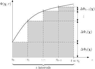
Figure 1. Time marching scheme

The discretization of the Equations (2.1) - (2.2) using constant spatial and constant temporal elements may be written as

$$\begin{split}\sum\limits_{\lambda=1}^{N}A_{xx}^{\beta\lambda}D_{s}^{\lambda,h}+\sum\limits_{\lambda=1}^{N}A_{xy}^{\beta\lambda}D_{n}^{\lambda,h}+\sum\limits_{\lambda=1}^{N}A_{xq}^{\beta\lambda}D_{q}^{\lambda,h}=\\ \sigma_{s}^{h}(x^{\beta},t)-\sum\limits_{\eta=0}^{h-1}\sum\limits_{\lambda=1}^{N}\bigg{(}A_{xx}^{\beta\lambda,\eta}D_{s}^{\lambda,\eta}+A_{xy}^{\beta\lambda,\eta}D_{n}^{\lambda,\eta}+A_{xq}^{\beta\lambda,\eta}D_{q}^{\lambda,\eta}\bigg{)},\end{split}$$ (2.3)

$$\begin{split}\sum\limits_{\lambda=1}^{N}A_{yx}^{\beta\lambda}D_{s}^{\lambda,h}+\sum\limits_{\lambda=1}^{N}A_{yy}^{\beta\lambda}D_{n}^{\lambda,h}+\sum\limits_{\lambda=1}^{N}A_{yq}^{\beta\lambda}D_{q}^{\lambda,h}=\\ \sigma_{n}^{h}(x^{\beta},t)-\sum\limits_{\eta=0}^{h-1}\sum\limits_{\lambda=1}^{N}\bigg{(}A_{yx}^{\beta\lambda,\eta}D_{s}^{\lambda,\eta}+A_{yy}^{\beta\lambda,\eta}D_{n}^{\lambda,\eta}+A_{yq}^{\beta\lambda,\eta}D_{q}^{\lambda,\eta}\bigg{)},\end{split}$$ (2.4)

$$\begin{split}\sum\limits_{\lambda=1}^{N}A_{px}^{\beta\lambda}D_{s}^{\lambda,h}+\sum\limits_{\lambda=1}^{N}A_{py}^{\beta\lambda}D_{n}^{\lambda,h}+\sum\limits_{\lambda=1}^{N}A_{pq}^{\beta\lambda}D_{q}^{\lambda,h}=\\ p_{p}^{h}(x^{\beta},t)-\sum\limits_{\eta=0}^{h-1}\sum\limits_{\lambda=1}^{N}\bigg{(}A_{px}^{\beta\lambda,\eta}D_{s}^{\lambda,\eta}+A_{py}^{\beta\lambda,\eta}D_{n}^{\lambda,\eta}+A_{pq}^{\beta\lambda,\eta}D_{q}^{\lambda,\eta}\bigg{)}.\end{split}$$ (2.5)

In Equations (2.3)-(2.5), $A_{ij}$ are the coefficients relating the displacement discontinuities and fluid sources to shear stress, normal stress and pore pressure (Carvalho, 1991). For example, $A_{xx}$ is the shear stress that is induced on the observation point from a unit shear displacement discontinuity at the influencing point. In general, the fracturing fluid pressure is known at the boundary of a hydraulic fracturing problem (i.e. fracture surface), and the fracture surface displacements and flow discontinuity are the unknowns. Therefore, Equations (2.3)-(2.5) form a set of $3N$ linear equations which may be solved for $3N$ unknowns namely $\sigma_{s}$, $\sigma_{n}$, and $p$ for a single time step. As it may be seen, totally nine matrix-vector multiplications exist on the right hand side of Equations (2.3)-(2.5). Moreover, for any extra time step that is added to the problem, nine matrix-vector multiplications will be added to the computation. Furthermore, using an iterative solver like GMRES requires nine matrix-vector multiplications at each iteration. These operations increase the computational time especially with a large number of spatial or temporal elements. Hence, to improve the computational efficiency, a fast multipole method is implemented in the PDDM algorithm. Rezaei et al (2017) applied the bbFMM to the double summation on the right hand-side of Equations (2.3) - (2.5). In this study, bbFMM is applied on both double summation and GMRES iterative solver. Details of FMM and its implementation are discussed in the following sections of the paper.

2.1. Calculation of Stress Intensity Factors

Two classes of parameters are required in order to determine if the fracture propagation occurs. The first parameter is the fracture toughness $K_{Ic}$, which measures the ability of a material containing a fracture to resist a load and is determined experimentally. The second set of parameters is given by the stress intensity factors (SIFs) (Irwin, 1957), which are a function of the fracture length and of the stress applied on the surface of the fracture.

Following the principles of linear elastic fracture mechanics (LEFM), a fracture may propagate according to three different modes: opening or tensile (mode I), plane shearing or sliding (mode II), out-of-plane shearing or tearing (mode III). There are three stress intensity factors associated with these different loading modes, known as $K_{I}$, $K_{II}$ and $K_{III}$, respectively. Among these three, only $K_{I}$ and $K_{II}$ are considered in 2D cases because they don’t involve the third dimension. The calculation of the stress intensity factors plays a critical role in mixed mode fracture propagation criteria. SIFs are usually calculated at the tip of the fracture. Olson (1990) empirically introduced a relationship for calculating the SIFs using $D_{n}$ and $D_{s}$ of the fracture tip element as

$$K_{I}=0.806\frac{E}{4(1-\nu^{2})}\sqrt{\frac{\pi}{2a}}D_{n}\,,\quad K_{II}=0.806\frac{E}{4(1-\nu^{2})}\sqrt{\frac{\pi}{2a}}D_{s}\,.$$ (2.6)

In this paper, our aim is to compare the accuracy of the calculated SIFs using either a conventional or a fast multipole version of a fully poroelastic DDM model.

3. Fast Multipole Method (FMM)

The Fast Multipole Method (FMM) is a method to efficiently calculate matrix-vector products of the type

$$f(\boldsymbol{x}_{i})=\sum_{j=1}^{N}G(\boldsymbol{x}_{i},\boldsymbol{y}_{j})\,b(\boldsymbol{y}_{j})\,,\quad i=1,\ldots,N\,,$$ (3.1)

using $O(N)$ operations and a controllable error. Here, the kernel function $G$ relates the influenced points $\boldsymbol{x}_{i}$ with the influencing points $\boldsymbol{y}_{j}$, $b(\boldsymbol{y}_{j})$ are the charges at the influencing points, and $f(\boldsymbol{x}_{i})$ is the potential at the influenced points. The main idea of FMM is to speed up the evaluation of the summation in (3.1) by using a hierarchical tree decomposition of the domain points. Thanks to this subdivision, a fast approximation of the kernel function can be introduced for large distances between the influencing and the influenced points, while the direct multiplication in (3.1) is used for points that are not well-separated.

3.1. Hierarchical Tree Decomposition

(a) Level 0

(b) Level 1

(c) Level 2

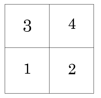
(d)

Figure 2. Hierarchical tree decomposition; (a) level 0 square, (b) level 1 square, (c) level 2 square, and (d) indexing convention

The hierarchical tree decomposition is the first step towards any fast multipole method. Figure 2 shows how this decomposition is performed in two dimensions, in which case it is also referred to as quad-tree structure. The square that covers the entire domain of the problem is called level 0 square (Figure 2a) and it is first divided into 4 child squares (Figure 2b) that define level 1. At any stage, any square that has more points than a prescribed number is recursively divided into 4 child squares and a new level is generated. Otherwise, the square is defined a leaf cell. In particular, a leaf cell that does not contain any points is called a zero cell. The process of cell subdivision stops when reaching a leaf cell. When new child cells are created, new indices must be assigned. Our convention is that the cell indexing increases from left to right and from bottom to top, as shown in Figure 2d. For example, the bottom left square and top right square at level 1 are the children number 1 and 4 of the level 0 square, respectively. It is worth mentioning that the indexing of cells is unrelated to the global numbering of the domain points.

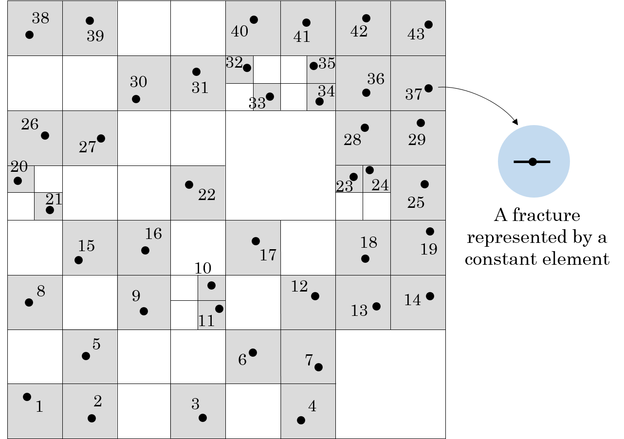
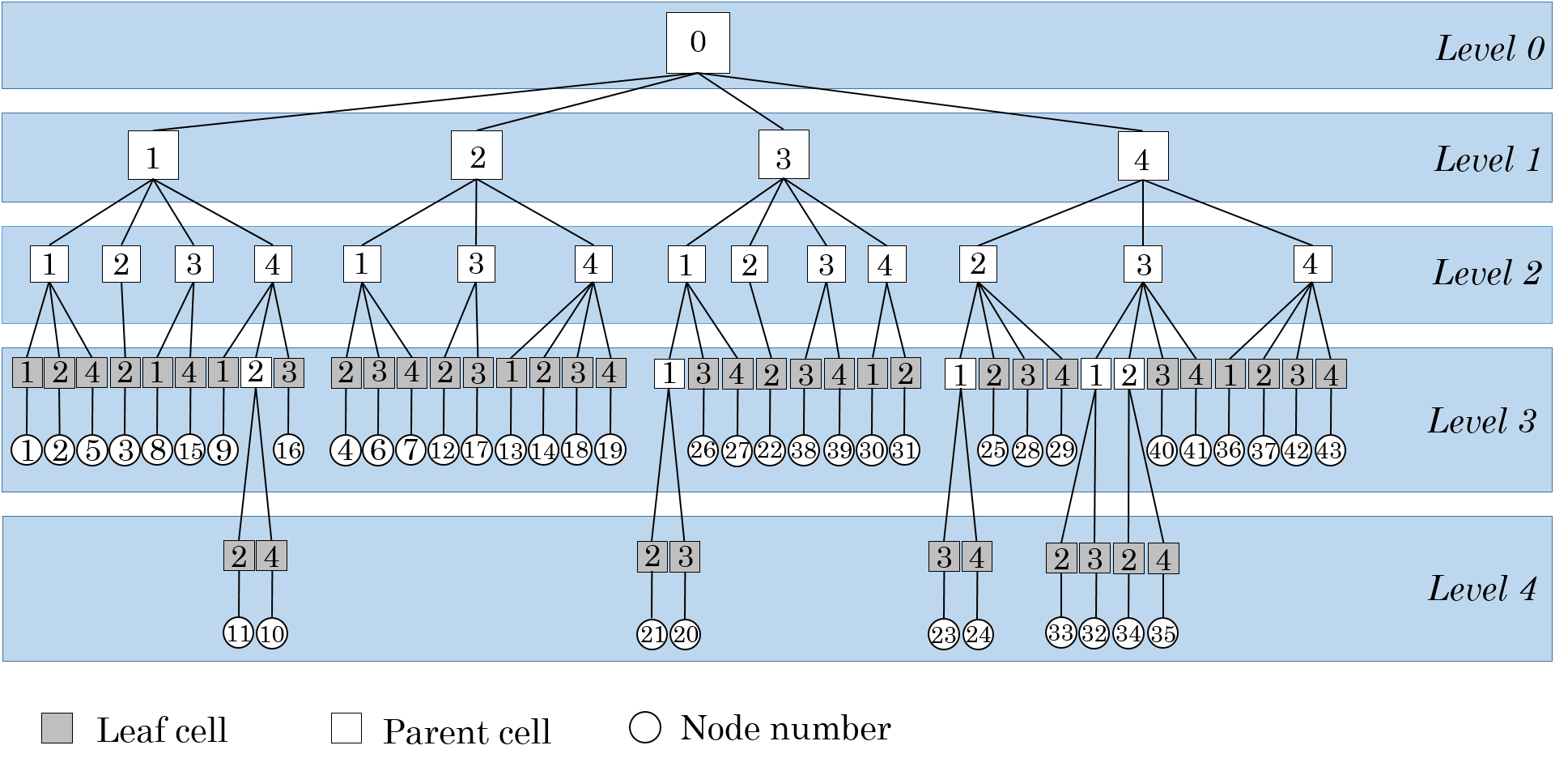
Figure 3. Top: an example with 43 randomly distributed points. Bottom: the associated hierarchical quad-tree structure.

To better explain the tree structure, Figure 3 at the top shows an example of a domain with 43 randomly distributed points. In the PDDM method, each of them represents the center point of a fracture element. The hierarchical tree for this example is shown in Figure 3. It summarizes the cell subdivisions as well as the relationships between cells and contained points. For example, child 2 and child 4 of level 0 have only three children each, because one of their children is a zero cell. Each point can be traced back to level 0 using the tree. For example, point number 21 belongs to the second child of the first child of the first child of the third child of the level 0 cell (i.e., the entire domain).

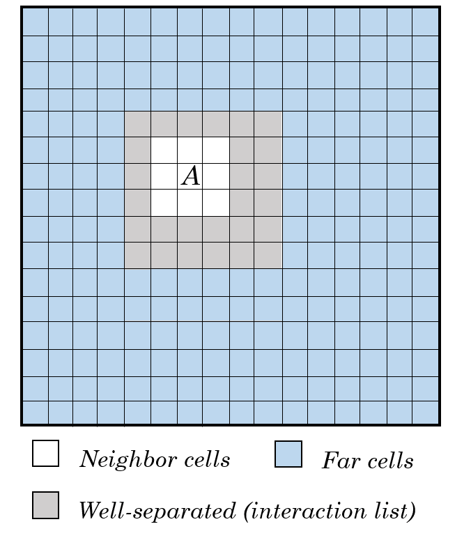
Figure 4. Three groups of cells associated with cell $A$

For each cell, three groups may be defined by using the tree structure:

• the list of neighbor cells, which are the cells at any level that have at least one common vertex with the given cell;

• the interaction list of the cell, which is made of all cells that are well-separated with respect to the given cell (two cells are said to be well-separated if they are not neighbors at the same level, but their parents are neighbors);

• the list of far cells, which are all the remaining cells in the domain.

Figure 4 shows an example of neighbor, well-separated, and far cells for cell $A$. In the example of Figure 3, the cells containing points 1 and 2 are neighbors, the cells containing points 1 and 3 are in the interaction lists of each other, and the cells containing point 1 and 43 are far cells. It should be noted that after the hierarchical tree structure is constructed, it will not change unless there is a change in the problem geometry such as fracture propagation. After its construction, the hierarchical tree can be used to calculate the potential at each point.

3.2. The Black-Box Fast Multipole Method

Different versions of the fast multipole method can be defined. We may distinguish them with respect to the way in which the kernel function is approximated. On one hand, we may consider expanding the kernel in terms of some analytical expansion (e.g. spherical harmonics expansion), and truncating such series. On the other, we may approximate the kernel through interpolation with respect to some basis. Fong and Darve (2009) introduced a version of the fast multipole method, called the black-box Fast Multipole Method, which belongs to the class of interpolation-based fast multipole methods. This method has several advantages compared to the ones based on an analytical kernel expansion. First of all, the method is black-box or kernel-independent in the sense that an analytical expansion of the kernel need not be known. Since the method is based on interpolation, only the evaluation of the kernel at certain points is required. Moreover, the interpolation is performed using Chebyshev polynomials, which have several advantages such as uniform convergence and near minimax approximation (Fong and Darve, 2009).

3.2.1. Kernel approximation with Chebyshev interpolation

For the sake of simplicity, let us describe the method in a one-dimensional domain. In this case, the corresponding two-dimensional kernel function $G(x,y)$ in Equation (3.1) is approximated by a low-rank approximation $\widetilde{G}(x,y)$ using polynomials $u_{l}$ and $v_{l}$, for $l=1,2,\ldots,n$,

$$\widetilde{G}(x,y)=\sum_{l=1}^{n}u_{l}(x)v_{l}(y)\,.$$ (3.2)

Combining Equations (3.2) and (3.1), a fast summation scheme for an approximation $\widetilde{f}$ of the potential $f$ is given by

$$\widetilde{f}(x_{i})=\sum_{l=1}^{n}u_{l}(x_{i})\sum_{j=1}^{N}v_{l}(y_{j})b(y_{j}).$$ (3.3)

Hence, first we transform the source charges using the second summation in the right-hand side of (3.3). Then, we calculate the influence at each observation point using the first summation. While the computational complexity of Equation (3.1) is $O(N^{2})$, a significant reduction is given by Equation (3.3) since in this case the complexity is $O(2nN)$, which is especially important when $n\ll N$.

Following Fong and Darve (2009), we choose Chebyshev polynomial interpolation for the low-rank kernel approximation (3.2). Given a function $g(x)$, the interpolating polynomial $p_{n-1}(x)$ of degree $n-1$ using Chebyshev polynomials $T_{k}$ can be written in the form (see Fong and Darve (2009))

$$p_{n-1}(x) =\sum_{l=1}^{n}g(\bar{x}_{l})\,S_{n}(\bar{x}_{l},x)\,,\text{ where }$$ (3.4)

$$S_{n}(x,y) =\dfrac{1}{n}+\dfrac{2}{n}\sum_{k=1}^{n-1}T_{k}(x)T_{k}(y)\,,$$ (3.5)

and $\bar{x}_{l}$ are the roots of $T_{n}$. Using this interpolating polynomial for both $u_{l}$ and $v_{l}$ in the low-rank approximation (3.2), the approximated kernel function $\widetilde{G}$ becomes

$$\widetilde{G}({x},{y})=\sum_{l=1}^{n}\sum_{m=1}^{n}G({\bar{x}_{l}},{\bar{y}_{m}})S_{n}({\bar{x}_{l}},{x})S_{n}({\bar{y}_{m}},{y})$$ (3.6)

Substituting this approximation into Equation (3.1), the fast summation method reads

$$\widetilde{f}(x_{i})=\sum_{j=1}^{N}\widetilde{G}(x_{i},y_{j})b(y_{j}) =\sum_{j=1}^{N}\bigg{[}\sum_{l=1}^{n}\sum_{m=1}^{n}G({\bar{x}_{l}},{\bar{y}_{m}})S_{n}({\bar{x}_{l}},x_{i})S_{n}({\bar{y}_{m}},y_{j})\bigg{]}b(y_{j})$$ (3.7)

$$=\sum_{l=1}^{n}S_{n}({\bar{x}_{l}},x_{i})\sum_{m=1}^{n}G({\bar{x}_{l}},{\bar{y}_{m}})\sum_{j=1}^{N}b(y_{j})S_{n}({\bar{y}_{m}},y_{j}).$$ (3.8)

First, one computes the weights at the Chebyshev nodes (summation over $j$ in (3.8)), then the approximated function $\widetilde{f}$ is computed at the Chebyshev nodes (summation over $m$), and finally $\widetilde{f}$ is calculated at the influenced points by interpolation (summation over $l$).

3.2.2. Upward Pass and Downward Pass

Using the hierarchical tree decomposition, clusters of particles are determined at different levels. The interaction between clusters that are well-separated are calculated using FMM, and the interaction between the clusters that are not well-separated are calculated using direct matrix-vector multiplication. Hence, two main steps have to be taken in order to compute potentials at each point: the upward pass and the downward pass.

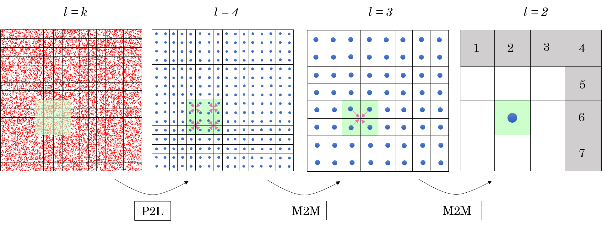
Figure 5. Upward pass

The algorithm starts with the upward pass (Figure 5), whose purpose is to construct weights at all levels for a subsequent evaluation of the potential. For each cell at all levels, the weights $W_{m}^{I}$ at the Chebyshev nodes $\bar{y}^{I}_{m}$ are calculated as (here we denote the set of child cells of a given cell $I$ as $\mathrm{Children}(I)$)

$$(l=k)\quad W_{m}^{I} =\sum_{y_{j}\in I}b(y_{j})S_{n}(\bar{y}^{I}_{m},y_{j}),\quad m=1,...,n\,,$$ (3.9)

$$(l=k-1,k-2,\ldots,1,0)\quad W_{m}^{I} =\sum_{J\in\mathrm{Children}(I)}\sum_{m^{\prime}}W_{m^{\prime}}^{J}S_{n}(\bar{y}^{I}_{m},\bar{y}_{m^{\prime}}^{J}),\quad m=1,...,n\,.$$ (3.10)

The interpolation at the finest level in (3.9) is called point-to-local (P2L) translation. All other levels are calculated recursively by moving through the tree upwards, from finer to coarser levels. Equation (3.10) is referred to as multipole-to-multipole (M2M) translation and consists of an interpolation of the weights from the child cells.

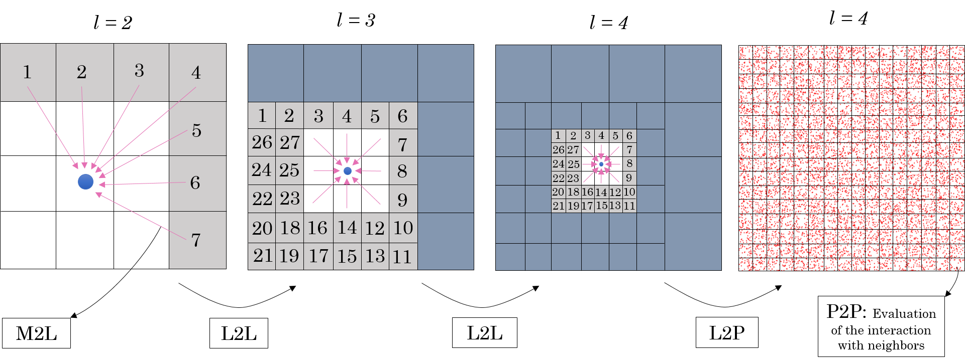
Figure 6. Downward pass

Then, the downward pass is performed for the final evaluation of the potential at the influenced points. This aims at treating differently the contributions to the potential coming from interaction list, far cells and neighbor cells. Figure 6 shows the steps that are required.

1) For a given cell $I$, the contributions at the Chebyshev nodes $\bar{x}_{m}^{I}$ to the potential field $f$ coming from the interaction list of $I$ are calculated by the following multipole-to-local (M2L) translation (let us denote with $\mathrm{IntList}(I)$ the interaction list of $I$)

$$(l=0,1,\ldots,k)\quad g_{m}^{I}=\sum_{J\in\mathrm{IntList}(I)}\sum_{m^{\prime}}W_{m^{\prime}}^{J}G(\bar{x}_{m}^{I},\bar{y}_{m^{\prime}}^{J}),\quad m=1,...,n\,.$$ (3.11)

2) In order to add the contributions from far cells on the current cell $I$, we travel the tree downwards to get

$$(l=0)\quad f_{m}^{I} =g_{m}^{I}\,,\quad m=1,...,n\,,$$ (3.12)

$$(l=1,2,\ldots k)\quad f_{m}^{I} =g_{m}^{I}+\sum_{l^{\prime}}f_{l^{\prime}}^{J}S_{n}(\bar{x}_{m}^{I},\bar{x}_{l^{\prime}}^{J}),\quad m=1,...,n\,.$$ (3.13)

Equation (3.13) is called local-to-local (L2L) interpolation based on the parent cell $J$ of $I$.

3) Finally, the approximation $\widetilde{f}$ of the potential is calculated at each influenced point of $I$ by adding two terms: the local-to-point (L2P) term, for the interpolation of the influences $f_{m}^{I}$ coming from both interaction list and far cells, and the point-to-point (P2P) term, to account for the self and neighbor interactions (we denote with $\mathrm{Neighb}(I)$ the list of neighbors of $I$)

$$(l=k)\quad\widetilde{f}(x_{i})=\sum_{m}f_{m}^{I}S_{n}(\bar{x}_{m}^{I},x_{i})+\sum_{J\in\mathrm{Neighb}(I)}\sum_{y_{j}\in J}b(y_{j})G(x_{i},y_{j})\,.$$ (3.14)

The procedure that was explained in this section can be implemented within a BEM algorithm such as the PDDM algorithm. This will be explained in the next section.

4. PDDM with FMM (FMPDDM)

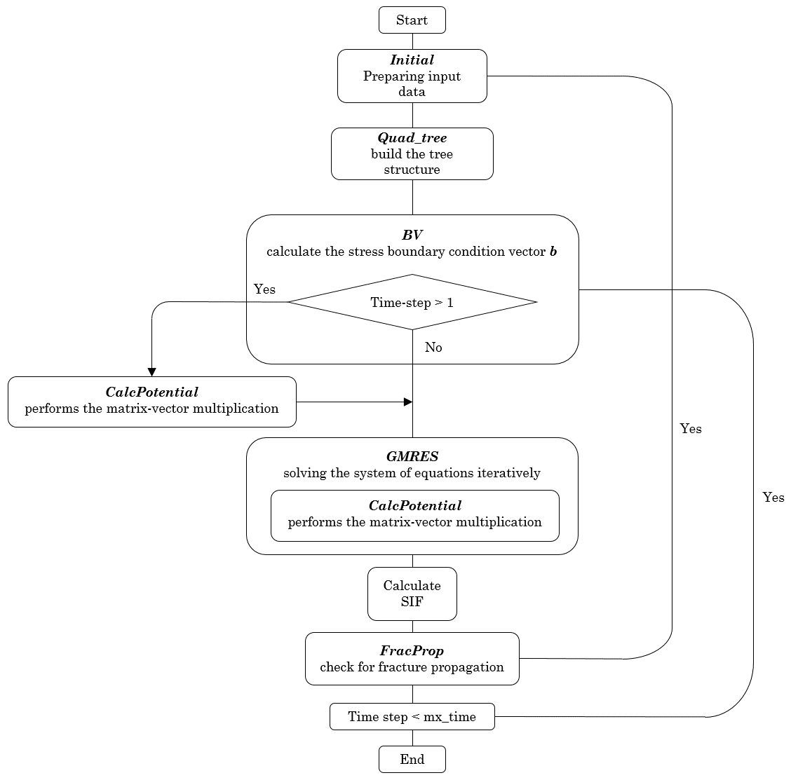
Figure 7. FMPDDM algorithm

The FMPDDM algorithm that is used in this study is shown in Figure 7. As it can be seen, the first step to obtain $D_{s}$, $D_{n}$ and $D_{q}$ is to provide the spatial, temporal and material poroelastic properties, and rock far-field stress and pore pressure, and the prescribed properties of the FMM model. Next, the quad-tree structure needs to be constructed. It should be noted that the tree structure remains constant as long as the geometry is the same (i.e no fracture propagation occurs). In the first time step, the right-hand side vector (i.e $\sigma_{s_{0}}$, $\sigma_{n_{0}}$, and $P_{p_{0}}$) is formed by transforming the far-field stresses to the face of each element and by adding their effect to the hydraulic load on the elements. For the time steps $t=2,...,\tau_{h}$ the solutions obtained from all of the previous time steps need to be subtracted from the known right-hand side vector to account for the term with double summation in Equations (2.3)-(2.5). For this purpose, the matrix-vector multiplication between the coefficient matrices and the solutions of the previous time steps is performed by using FMM. Finally, a modified version of GMRES with FMM for matrix-vector multiplication is used to iteratively solve for the problem unknowns.

After obtaining the solutions, one may calculate the SIFs mode-I and II using Equation (2.6). Then, a fracture propagation criterion may be used to check to see whether the propagation criterion is satisfied. Consequently, an element will be added to the model if propagation happens, and in that case the quad-tree needs to be constructed again. In the case of no propagation, the solution of later time steps is obtained by marching in time until reaching the final time step.

5. Numerical results

Some examples are presented here to demonstrate the application of the method. The aim is to compare the accuracy and computational time of FMPDDM versus PDDM. The properties of Westerly granite used as input data for all the subsequent examples are shown in Table 1. The properties that are required for the model are shear modulus $G$, drained and undrained Poisson ratios $\nu$ and $\nu_{d}$, Skemptson’s coefficient $B$, diffusivity coefficient $c$, permeability $k$, and Biot’s poroelasticity coefficient, $\alpha$.

Rock type	$G$	$\nu$	$\nu_{u}$	$B$	$c$	$k$	$\alpha$
	$GPa$	$-$	$-$	$-$	$m^{2}/s$	$m^{2}$	$-$
Westerly granite	$15$	$0.25$	$0.331$	$0.81$	$6.15\cdot 10^{-5}$	$4\cdot 10^{-19}$	$0.449$

Table 1. Rock poroelastic properties used in this study (adopted from Cheng (2016)).

5.1. Dependence on the number of fracture elements

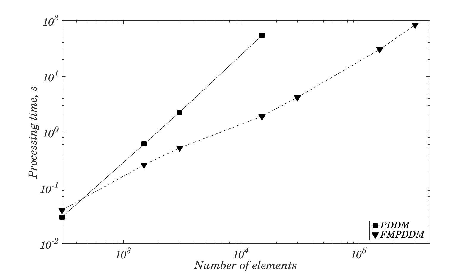
Figure 8. CPU processing time vs. number of elements for one time step

First, the processing times of the two methods are compared as a function of the number of boundary elements. The comparison for one time step of the solution is shown in Figure 8. Initially PDDM performs better in terms of processing time, but, as the number of elements increases, it takes more time for the PDDM method to solve a problem with the same number of elements in one time step. By further increasing the number of elements, the slope of PDDM becomes equal to two, while the FMPDDM has the slope of one. This indicates that PDDM has the complexity of $O(N^{2})$, while FMPDDM has the complexity of $O(N)$.

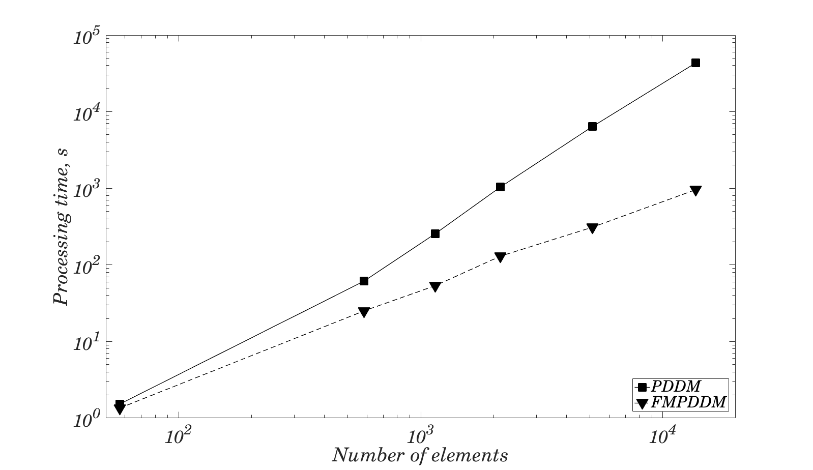
Figure 9. CPU processing time vs. number of elements for 10 time steps

Figure 9 shows the processing times for 10 time steps with the same time discretization as a function of the number of elements. As required by the time marching method, for all time steps other than the first time step, it is necessary to subtract all the previous solutions from the current time step boundary condition (Equations (2.3)-(2.5)). This creates extra steps with matrix-vector multiplications, increasing the processing time even further. As it may be seen in the figure, as the number of elements increases, FMPDDM performs much better than PDDM in terms of processing time. For example, for $13682$ elements it was observed that the processing time of the PDDM method was about $43340$ seconds, while for the same problem it took only $960$ seconds for the FMPDDM to calculate the solution. This is a huge difference in processing time ($\sim 40$ times less). Also, a better performance is expected for greater number of elements.

5.2. Accuracy of the solution

Another important aspect to investigate for FMDDM is to see how the accuracy of the solution is preserved. In order to investigate this feature, two examples are investigated. In the first example, a hydraulic fracturing problem in a horizontal well is studied. In the second example, the problem of randomly distributed pressurized fractures is presented. For each case, shear and normal displacements of a certain element as well as its stress intensity factors $K_{I}$ and $K_{II}$ are calculated. For each case, the accuracy is discussed along with the factors that may be used to improve it.

5.2.1. Transverse Hydraulic Fractures in a Cluster

It is a common practice in the oil industry to drill a well horizontally and initiate multiple hydraulic fractures to increase the hydrocarbon production. In most of the ultra-tight reservoirs, hydrocarbon recovery is impossible without hydraulic fractures. Figure 10a shows a schematic of the hydraulic fracture process in a horizontal wellbore. Usually, the well is drilled parallel to the minimum horizontal stress direction and multiple sections of the wellbore are isolated and perforated from the “toe” of the horizontal well to its “heel”. This causes hydraulic fractures to initiate and propagate orthogonal to the wellbore (i.e. parallel to the direction of maximum horizontal compressional stress). Consequently, new interface areas are created inside the reservoir that cause an increase in the production of hydrocarbon from wellbore.

In order to show the accuracy of the proposed algorithm, the solution of five parallel hydraulic fractures in a horizontal well is studied. Figure 10b shows the geometry of the problem that is used for this purpose. Five parallel hydraulic fractures, each having $400\,m$ half-length (hydraulic length) are assumed. Each fracture is discretized using $200$, $300$, and $400$ constant DDM elements.

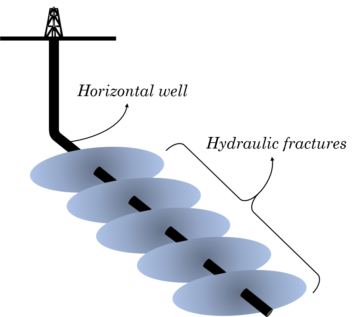
(a)

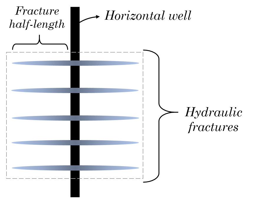
(b)

Figure 10. Hydraulic fracturing in a horizontal well; a) 3D view, b) top view

The boundary condition and the other inputs of the model are summarized in Table 2. For this problem, we assume that the directions of maximum and minimum horizontal stresses are $x$ and $y$, respectively. The spacing of each fracture is also chosen to be $30\;m$. The fluid is injected into the wellbore with $58\;MPa$ and the problem is solved for the first time step equal to $100\;s$.

Maximum horizontal stress, $\sigma_{H}$	$58.60\text{ MPa}$
Minimum horizontal stress, $\sigma_{h}$	$55.15\text{ MPa}$
Initial reservoir pore pressure, $p_{0}$	$48.26\text{ MPa}$
Injection pressure, $p_{i}$	$58\text{ MPa}$
Fracture spacing	$30\text{m}$
Fracture half-length, $a$	$400\text{m}$

Table 2. Model configuration for hydraulic fractures in a horizontal wellbore

In order to compare the accuracy of the model, we have chosen four elements and compared the shear and normal displacements on these elements using FMPDDM and PDDM. The center elements and tip elements of the inner and outer fracture (third and fifth fracture from the top in Figure 10b). are the elements that we chose for this purpose. The number of Chebyshev nodes is set to 6 for this example. Table 3 shows the normal displacement of the center element and tip element of the inner fracture for different discretizations of $200$, $300$, and $500$ up to four decimal places for each fracture respectively.

$D_{n}$	Fracture center			Fracture tip
NE	$1000$	$1500$	$2000$	$1000$	$1500$	$2000$
Max. level	2	3	3	2	3	3
PDDM	$0.0199$	$0.0184$	$0.0170$	$0.0049$	$0.0040$	$0.0034$
FMPDDM	$0.0193$	$0.0179$	$0.0166$	$0.0047$	$0.0039$	$0.0033$
error (%)	$-3$	$-2.7$	$-2.3$	$-4$	$2.5$	$-2.9$

Table 3. Normal displacement of the inner fracture surface for different number of elements (NE) after the first time step

As it may be seen in the Table 3, the normal opening of the fracture at the center is higher as expected. Also, the maximum error that is reported for normal displacements is smaller than 4% for all cases. Also, it should be noted that the results that are obtained by FMPDDM are smaller than the results that are obtained by PDDM. Shear displacements at the center and tip of the fracture were smaller than the tolerance of GMRES ($=10^{-6}$). This was expected because having any shear displacement on the elements in the middle fracture causes a mixed mode (mode I + II) fracture propagation. This is not the case for such an arrangement as was shown previously. Therefore, we didn’t report the shear displacement of the center fracture for this case. Similar calculation may be done for the outer fracture. Table 4 shows the normal displacement of the outer fracture.

$D_{n}$	Fracture center			Fracture tip
NE	$1000$	$1500$	$2000$	$1000$	$1500$	$2000$
PDDM	$0.0198$	$0.0183$	$0.0170$	$0.0057$	$0.0044$	$0.0037$
FMPDDM	$0.0192$	$0.0178$	$0.0166$	$0.0056$	$0.0043$	$0.0036$
error (%)	$-3$	$-2.7$	$-2.3$	$-1.75$	$-2.27$	$-2.7$

Table 4. Normal displacement of the outer fracture surface for different number of elements (NE) after the first time step

Similar to what was observed for the inner fracture normal displacement, the error of the normal displacement on the outer fracture was smaller than 4%. Also, as expected, both shear and normal openings of the outer fracture were bigger compared to the inner fracture. This is because the stress shadow that is created by other outer fractures impedes the inner fracture from opening. Next, shear displacement of the outer fracture is presenter in Table 5. For the same reason that explained in the case of inner fracture shear displacement, only the shear displacement of one of the outer fracture tips is presented here.

$D_{s}$	Fracture tip
NE	$1000$	$1500$	$2000$
PDDM	$0.0024$	$0.0019$	$0.0015$
FMPDDM	$0.0023$	$0.0018$	$0.0015$
error (%)	$-4.16$	$-5$	$0$

Table 5. Shear displacement of the outer fracture surface for different number of elements (NE) after the first time step (Note: the shear displacement of the fracture center was less than machine precision).

As shown in Table 5, the same error was also observed for the shear displacement of the outer fracture. Also, it was expected that because of stress shadowing effect, some shear will be observed at the tip of the outer fracture since the outer fractures tend to reorient away from the middle fractures. As shown in this example using FMPDDM will give acceptable results with smaller computation time. The error was smaller than 4% in all of the cases. As an example, the processing time required for FMPDDM to solve the $2000$ element case ($400$ element per fracture) was one third of the time required for PDDM to solve the same problem. Next, we present a case of randomly distributed fractures and do the same exercise while giving different angles to the distributed fractures.

5.2.2. Randomly Distributed Pressurized Fractures

Underground rocks are discontinuous media filled with natural fractures. Thus, it is necessary to include them in any hydraulic fracturing study. In this section, randomly distributed pressurized fractures are studied to analyze the accuracy of the developed FMPDDM. Here, we assume that all fractures are pressurized. Similar to the previous section, we choose one fracture here and calculate the normal and shear displacements of both tips. Then, we calculate mode I and II stress intensity factors that are crucial for any fracture propagation study.

Figure 11 shows the geometry of the problem that is studied in this section. The fracture that is selected for the displacement calculation is shown on the figure (fracture A). Fracture A has five elements. It is also assumed that all fractures are parallel to each other and three cases with different angles of $15^{o}$, $45^{o}$, $75^{o}$ with respect to the $x$ axis are considered. The direction of maximum and minimum horizontal stresses in all cases are $x$ and $y$, respectively.

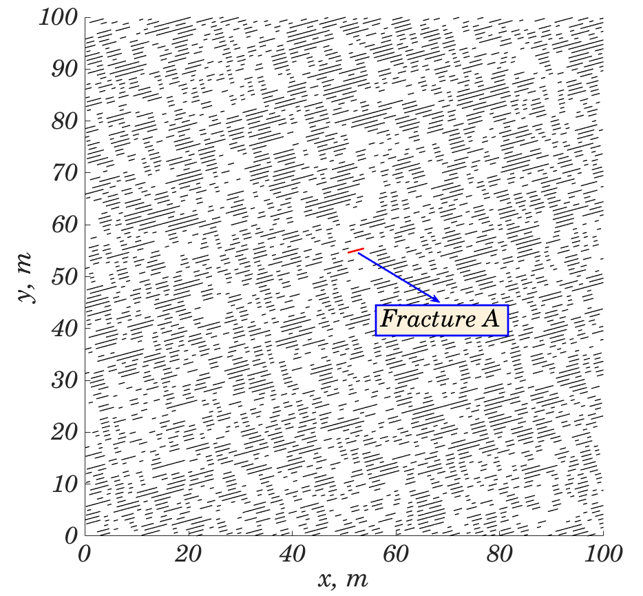
(a) $15^{o}$

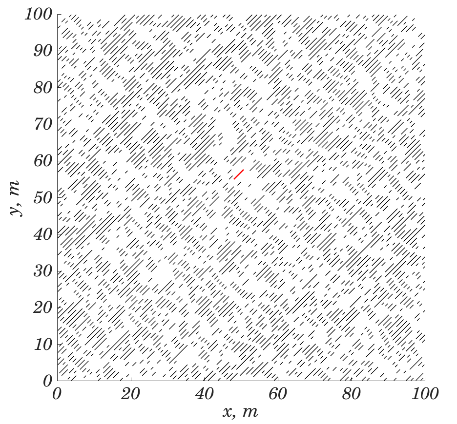
(b) $45^{o}$

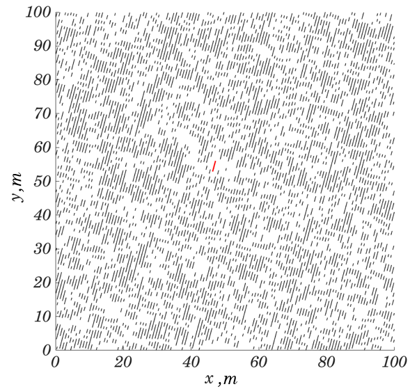
(c) $75^{o}$

Figure 11. Randomly distributed fractures (angles are with respect to maximum ($x$ axis) horizontal stress).

Table 6 represents the boundary conditions and the other input variables of the model. The injection pressure in this case is $60\;MPa$ to make sure all the fractures are open. Time is discretized into one time step equal to $10$ seconds. Also, to increase the accuracy of FMPDDM, Chebyshev polynomials of degrees three (NCheb3) and six (NCheb6) are chosen. The processing times of PDDM, FMPDDM-NCheb6, and FMPDDM-NCheb3 observed as 8050, 421, and 120 seconds, respectively. Therefore, the processing time can be cut by almost 67 times.

Maximum horizontal stress, $\sigma_{H}$	$58.60\text{ MPa}$
Minimum horizontal stress, $\sigma_{h}$	$55.15\text{ MPa}$
Reservoir pore pressure, $p_{r}$	$48.26\text{ MPa}$
Pressure inside the fracture, $p_{f}$	$60\text{ MPa}$
Number of fractures	$4335$
Number of elements	$20332$
Number of fracture A elements	$5$

Table 6. Input parameters of the randomly distributed pressurized fractures.

Table 7 shows the shear displacements at the right and left tips of fracture $A$ for different angles. Comparing PDDM, FMPDDM-NCheb3, and FMPDDM-NCheb6 shows that, although using the FMPDDM-NCheb3 requires only two minutes compared with more than two hours required with PDDM, it causes a small error in the solution. The error may be reduced by using FMPDDM-NCheb6, but it increases the computational time to $7$ minutes, which is still much less than the run time required for PDDM.

$D_{s}$	Fracture left tip $\times 10^{-5}$ m			Fracture right tip $\times 10^{-5}$ m
Angle	$15^{o}$	$45^{o}$	$75^{o}$	$15^{o}$	$45^{o}$	$75^{o}$
Conventional PDDM	$2.0592$	$7.2157$	$2.6829$	$4.6915$	$8.1299$	$2.6438$
FMPDDM-NCheb3	$2.0545$	$7.2050$	$2.6795$	$4.6736$	$8.1307$	$2.6478$
FMPDDM-NCheb6	$2.0594$	$7.2155$	$2.6829$	$4.6915$	$8.1298$	$2.6438$

Table 7. Shear displacement of the tips of fracture $A$

The same calculation for the normal displacement of fracture $A$ tips is presented in Table 8. Similar to shear displacement, the same error was observed for this case. In both cases, the relative error in calculating the displacement is in the order of $10^{-3}$, and FMPDDM-NCheb3 error is four times bigger than FMPDDM-NCheb6. The error for both cases is negligible, and as it will be discussed in the next section, it will not change the SIF calculation, which is the key part for calculating the fracture propagation.

$D_{n}$	Fracture left tip $\times 10^{-5}$ m			Fracture right tip $\times 10^{-5}$ m
Angle	$15^{o}$	$45^{o}$	$75^{o}$	$15^{o}$	$45^{o}$	$75^{o}$
Conventional PDDM	$2.2694$	$11.733$	$1.2616$	$12.227$	$11.443$	$0.8101$
FMPDDM-NCheb3	$2.3158$	$11.704$	$1.2612$	$12.246$	$11.460$	$0.8113$
FMPDDM-NCheb6	$2.2697$	$11.733$	$1.2616$	$12.227$	$11.443$	$0.8101$

Table 8. Normal displacement of fracture $A$

The accuracy and speed of the PDDM and two FMPDDMs via two examples were presented in this section. The relative errors for the case of parallel fractures was calculated to be less than $4$%. The reason for the big differences in the error is that in the first example, elements were not evenly distributed on a plane, whereas in the second example points where distributed on the plane. In the next section, the stress intensity factor for the right tip of fracture $A$ is calculated using FMPDDM with two different degrees, and the results are compared to the stress intensity factor calculated using the PDDM.

The stress intensity factor calculation is the key part of any fracture propagation investigation. Any error in the calculation of SIF results in erroneous determination of both angle (if considering mixed mode I+II) and the moment of fracture extension. In order to investigate the accuracy of the developed FMPDDM model, the SIF calculation on the right tip of fracture $A$ is conducted. Table 9 shows the result of this calculation. The error of FMPDDM-NCheb6 is less than $10^{-4}$ for this problem.

	$SIF_{I}$, $MPa\sqrt{m}$			$SIF_{II}$, $MPa\sqrt{m}$
Angle	$15^{o}$	$45^{o}$	$75^{o}$	$15^{o}$	$45^{o}$	$75^{o}$
Conventional PDDM	$3.0304$	$2.8362$	$0.20078$	$1.1628$	$2.0150$	$0.65527$
FMPDDM-NCheb3	$3.0352$	$2.8405$	$0.20109$	$1.1584$	$2.0152$	$0.65627$
FMPDDM-NCheb6	$3.0305$	$2.8362$	$0.20078$	$1.1628$	$2.0150$	$0.65527$

Table 9. Stress intensity factor mode II ($K_{II}$) at the right tip of fracture $A$

The errors of SIF calculated by FMPDDM using both polynomials of degree 3 and 6 are small enough and do not cause an error in the calculation of the angle and the moment of fracture extension. Fracture propagation is subject of future investigations.

6. Conclusions

In this study, a kernel-independent fully-poroelastic fast multipole displacement discontinuity model was developed to study hydraulic fracturing problems. The FMM uses Chebyshev polynomials for the kernel expansion. Dependence of the model performance to number of elements is compared with the conventional fully-poroelastic DDM for one kernel matrix-vector multiplication, and a complete hydraulic fracture problem including 10 time steps. Also, in order to compare the accuracy of the developed method, its performance was compared with a conventional displacement discontinuity method using two examples. In the first example the injection of the fracturing fluid into five parallel hydraulic fractures in a horizontal well was studied. It was observed that the maximum error in the shear and normal displacements of the fracture surfaces at the wellbore and fracture tips is less than $5$%. This error may be further minimized by choosing higher order Chebyshev polynomials. Generally, choosing higher order polynomials requires more computational time. In the second example, the problem of randomly pressurized fractures was considered. The error in this case was about $0.5$%. The difference between the error in the two examples is due to the distribution of the elements in the plane in the second example. In the first example, points were on the fractures, while in the second example points were distributed randomly in the plane. The results show that hydraulic fracture problems may be solved up to approximately 70 times faster by incorporating the fast multipole method into the conventional poroelastic displacement discontinuity method for a case of 2000 elements and one time step. Increasing the number of elements or time steps will make the ratio even bigger. We also showed that the error introduced by FMM in the solution is small enough that it has no significant effect on the SIF calculation, while decreasing the processing time. Therefore, fracture propagation angle and its occurrence moment can be estimated with high degree of confidence with FMPDDM. Although using higher order polynomials will affect the processing time and accuracy of the solution with FMPDDM, there are some other key factors such as iterations number in GMRES, degree of Chebyshev polynomials, tolerance of the GMRES, and distribution of the elements in a plane that also affect the results. In the next part of this study, the propagation of fractures will be studied using the SIFs that were calculated in this paper.

References

- Aliabadi and Rooke (1991) Aliabadi MH, Rooke D (1991) The boundary element method. Numerical Fracture Mechanics pp 90–139
- Alpert et al (1993) Alpert B, Beylkin G, Coifman R, Rokhlin V (1993) Wavelet-like bases for the fast solution of second-kind integral equations. SIAM Journal on Scientific Computing 14(1):159–184
- Banerjee and Butterfield (1981) Banerjee PK, Butterfield R (1981) Boundary element methods in engineering science, vol 17. McGraw-Hill London
- Biot (1941) Biot MA (1941) General theory of three-dimensional consolidation. Journal of applied physics 12(2):155–164
- Bobet and Mutlu (2005) Bobet A, Mutlu O (2005) Stress and displacement discontinuity element method for undrained analysis. Engineering fracture mechanics 72(9):1411–1437
- Carvalho (1991) Carvalho JL (1991) Poroelastic effects and influence of material interfaces on hydraulic fracture behaviour. PhD thesis, University of Toronto
- Cheng (2016) Cheng AHD (2016) Poroelasticity, vol 27. Springer, switzerland
- Cheng and Bunger (2016) Cheng C, Bunger AP (2016) Rapid simulation of multiple radially growing hydraulic fractures using an energy-based approach. International Journal for Numerical and Analytical Methods in Geomechanics 40(7):1007–1022
- Cheng et al (2005) Cheng H, Gimbutas Z, Martinsson PG, Rokhlin V (2005) On the compression of low rank matrices. SIAM Journal on Scientific Computing 26(4):1389–1404
- Cleary (1977) Cleary MP (1977) Fundamental solutions for a fluid-saturated porous solid. International Journal of Solids and Structures 13(9):785–806
- Cleary (1980) Cleary MP (1980) Comprehensive design formulae for hydraulic fracturing. In: SPE Annual Technical Conference and Exhibition, Society of Petroleum Engineers
- Crouch (1976) Crouch S (1976) Solution of plane elasticity problems by the displacement discontinuity method. i. infinite body solution. International Journal for Numerical Methods in Engineering 10(2):301–343
- Cruse (2012) Cruse TA (2012) Boundary element analysis in computational fracture mechanics, vol 1. Springer Science & Business Media
- Curran and Carvalho (1987) Curran J, Carvalho JL (1987) A displacement discontinuity model for fluid-saturated porous media. In: 6th ISRM Congress, International Society for Rock Mechanics
- Dahmen et al (2006) Dahmen W, Harbrecht H, Schneider R (2006) Compression techniques for boundary integral equations—asymptotically optimal complexity estimates. SIAM journal on numerical analysis 43(6):2251–2271
- Detournay and Cheng (1987) Detournay E, Cheng AH (1987) Poroelastic solution of a plane strain point displacement discontinuity. Journal of applied mechanics 54(4):783–787
- Detournay et al (1989) Detournay E, Cheng AD, Roegiers JC, Mclennan JD (1989) Poroelasticity considerations in in situ stress determination by hydraulic fracturing. In: International Journal of Rock Mechanics and Mining Sciences & Geomechanics Abstracts, Elsevier, vol 26, pp 507–513
- Farmahini-Farahani and Ghassemi (2015) Farmahini-Farahani M, Ghassemi A (2015) Analysis of fracture network response to fluid injection. In: Proc. 40th Workshop on Geothermal Reservoir Engineering
- Farmahini-Farahani and Ghassemi (2016) Farmahini-Farahani M, Ghassemi A (2016) Simulation of micro-seismicity in response to injection/production in large-scale fracture networks using the fast multipole displacement discontinuity method (fmddm). Engineering Analysis with Boundary Elements 71:179–189
- Fong and Darve (2009) Fong W, Darve E (2009) The black-box fast multipole method. Journal of Computational Physics 228(23):8712–8725
- Ghassemi et al (2013) Ghassemi A, Zhou X, Rawal C (2013) A three-dimensional poroelastic analysis of rock failure around a hydraulic fracture. Journal of Petroleum Science and Engineering 108:118–127
- Gimbutas and Rokhlin (2003) Gimbutas Z, Rokhlin V (2003) A generalized fast multipole method for nonoscillatory kernels. SIAM Journal on Scientific Computing 24(3):796–817
- Gimbutas et al (2001) Gimbutas Z, Greengard L, Minion M (2001) Coulomb interactions on planar structures: inverting the square root of the laplacian. SIAM Journal on Scientific Computing 22(6):2093–2108
- Greengard and Rokhlin (1987) Greengard L, Rokhlin V (1987) A fast algorithm for particle simulations. Journal of computational physics 73(2):325–348
- Greengard (1987) Greengard LF (1987) The rapid evaluation of potential fields in particle systems. PhD thesis, New Haven, CT, USA, aAI8727216
- Guo et al (2014) Guo Z, Liu Y, Ma H, Huang S (2014) A fast multipole boundary element method for modeling 2-d multiple crack problems with constant elements. Engineering Analysis with Boundary Elements 47:1–9
- Helsing (2000) Helsing J (2000) Fast and accurate numerical solution to an elastostatic problem involving ten thousand randomly oriented cracks. International Journal of Fracture 100(4):321–327
- Howard and Fast (1970) Howard GC, Fast CR (1970) Hydraulic fracturing. New York, Society of Petroleum Engineers of AIME, 1970 210 P
- Irwin (1957) Irwin GR (1957) Analysis of stresses and strains near the end of a crack traversing a plate. J appl Mech
- Jaswon (1963) Jaswon M (1963) Integral equation methods in potential theory. i. Proc R Soc Lond A 275(1360):23–32
- Lai and Rodin (2003) Lai YS, Rodin GJ (2003) Fast boundary element method for three-dimensional solids containing many cracks☆. Engineering analysis with boundary elements 27(8):845–852
- Liu (2009) Liu Y (2009) Fast multipole boundary element method: theory and applications in engineering. Cambridge university press
- Liu and Li (2014) Liu Y, Li Y (2014) Revisit of the equivalence of the displacement discontinuity method and boundary element method for solving crack problems. Engineering Analysis with Boundary Elements 47:64–67
- Liu and Nishimura (2006) Liu Y, Nishimura N (2006) The fast multipole boundary element method for potential problems: a tutorial. Engineering Analysis with Boundary Elements 30(5):371–381
- Liu et al (2011) Liu Y, Mukherjee S, Nishimura N, Schanz M, Ye W, Sutradhar A, Pan E, Dumont NA, Frangi A, Saez A (2011) Recent advances and emerging applications of the boundary element method. Applied Mechanics Reviews 64(3):030,802
- Liu et al (2017) Liu Y, Li Y, Xie W (2017) Modeling of multiple crack propagation in 2-d elastic solids by the fast multipole boundary element method. Engineering Fracture Mechanics 172:1–16
- Martinsson and Rokhlin (2007) Martinsson PG, Rokhlin V (2007) An accelerated kernel-independent fast multipole method in one dimension. SIAM Journal on Scientific Computing 29(3):1160–1178
- Morris and Blair (2000) Morris JP, Blair SC (2000) An efficient displacement discontinuity method using fast multipole techniques. In: 4th North American Rock Mechanics Symposium, American Rock Mechanics Association
- Nishimura (2002) Nishimura N (2002) Fast multipole accelerated boundary integral equation methods. Applied Mechanics Reviews 55(4):299–324
- Nishimura et al (1999) Nishimura N, Yoshida Ki, Kobayashi S (1999) A fast multipole boundary integral equation method for crack problems in 3d. Engineering Analysis with Boundary Elements 23(1):97–105
- Olson (1990) Olson JE (1990) Fracture mechanics analysis of joints and veins. PhD thesis, Stanford University
- Otani and Nishimura (2008) Otani Y, Nishimura N (2008) An fmm for periodic boundary value problems for cracks for helmholtz’equation in 2d. International journal for numerical methods in engineering 73(3):381–406
- Peirce (2016) Peirce A (2016) Implicit level set algorithms for modelling hydraulic fracture propagation. Phil Trans R Soc A 374(2078):20150,423
- Peirce and Bunger (2014) Peirce A, Bunger A (2014) Robustness of interference fractures that promote simultaneous growth of multiple hydraulic fractures. In: 48th US Rock Mechanics/Geomechanics Symposium, American Rock Mechanics Association
- Peirce and Napier (1995) Peirce AP, Napier J (1995) A spectral multipole method for efficient solution of large-scale boundary element models in elastostatics. International Journal for Numerical Methods in Engineering 38(23):4009–4034
- Rezaei et al (2017) Rezaei A, Siddiqui F, Bornia G, Soliman M, Rafiee M, Morse S (2017) A novel approach to efficiently solve displacement discontinuity problems in poroelastic media. In: 51th US Rock Mechanics/Geomechanics Symposium, American Rock Mechanics Association
- Rezaei et al (2018) Rezaei A, Bornia G, Rafiee M, Soliman M, Morse S (2018) Analysis of refracturing in horizontal wells: Insights from the poroelastic displacement discontinuity method. International Journal for Numerical and Analytical Methods in Geomechanics pp 1–22
- Rizzo (1967) Rizzo FJ (1967) An integral equation approach to boundary value problems of classical elastostatics. Quarterly of applied mathematics 25(1):83–95
- Rokhlin (1985) Rokhlin V (1985) Rapid solution of integral equations of classical potential theory. Journal of computational physics 60(2):187–207
- Safari and Ghassemi (2014) Safari R, Ghassemi A (2014) 3d coupled poroelastic analysis of multiple hydraulic fractures. In: 48th US Rock Mechanics/Geomechanics Symposium, American Rock Mechanics Association
- Schanz (2018) Schanz M (2018) Fast multipole method for poroelastodynamics. Engineering analysis with boundary elements 89:50–59
- Vandamme and Roegiers (1990) Vandamme LM, Roegiers JC (1990) Poroelasticity in hydraulic fracturing simulators. Journal of Petroleum Technology 42(09):1–199
- Verde and Ghassemi (2013a) Verde A, Ghassemi A (2013a) Efficient solution of large-scale displacement discontinuity problems using the fast multipole method. In: 47th US Rock Mechanics/Geomechanics Symposium, American Rock Mechanics Association
- Verde and Ghassemi (2013b) Verde A, Ghassemi A (2013b) Fracture network response to injection using an efficient displacement discontinuity method. In: 37th Annual meeting Geothermal Resources Council (GRC)
- Verde and Ghassemi (2015a) Verde A, Ghassemi A (2015a) Fast multipole displacement discontinuity method (fm-ddm) for geomechanics reservoir simulations. International Journal for Numerical and Analytical Methods in Geomechanics 39(18):1953–1974
- Verde and Ghassemi (2015b) Verde A, Ghassemi A (2015b) Modeling injection/extraction in a fracture network with mechanically interacting fractures using an efficient displacement discontinuity method. International Journal of Rock Mechanics and Mining Sciences 77:278–286
- Verde and Ghassemi (2016) Verde A, Ghassemi A (2016) Large-scale poroelastic fractured reservoirs modeling using the fast multipole displacement discontinuity method. International Journal for Numerical and Analytical Methods in Geomechanics 40(6):865–886
- Wang and Yao (2011) Wang H, Yao Z (2011) A fast multipole dual boundary element method for the three-dimensional crack problems. Computer Modeling in Engineering & Sciences(CMES) 72(2):115–147
- Wang et al (2005) Wang P, Yao Z, Wang H (2005) Fast multipole bem for simulation of 2-d solids containing large numbers of cracks. Tsinghua Science & Technology 10(1):76–81
- Weng (2015) Weng X (2015) Modeling of complex hydraulic fractures in naturally fractured formation. Journal of Unconventional Oil and Gas Resources 9:114–135
- Wu and Olson (2015) Wu K, Olson JE (2015) Simultaneous multifracture treatments: fully coupled fluid flow and fracture mechanics for horizontal wells. SPE journal 20(02):337–346
- Ying et al (2004) Ying L, Biros G, Zorin D (2004) A kernel-independent adaptive fast multipole algorithm in two and three dimensions. Journal of Computational Physics 196(2):591–626
- Yokota et al (2016) Yokota R, Ibeid H, Keyes D (2016) Fast multipole method as a matrix-free hierarchical low-rank approximation. arXiv preprint arXiv:160202244
- Yoshida et al (2001) Yoshida Ki, Nishimura N, Kobayashi S (2001) Application of fast multipole galerkin boundary integral equation method to elastostatic crack problems in 3d. International Journal for Numerical Methods in Engineering 50(3):525–547