Features Extraction Based on an Origami Representation of 3D Landmarks

Abstract

Feature extraction analysis has been widely investigated during the last decades in computer vision community due to the large range of possible applications. Significant work has been done in order to improve the performance of the emotion detection methods. Classification algorithms have been refined, novel preprocessing techniques have been applied and novel representations from images and videos have been introduced. In this paper, we propose a preprocessing method and a novel facial landmarks’ representation aiming to improve the facial emotion detection accuracy. We apply our novel methodology on the extended Cohn-Kanade (CK+) dataset and other datasets for affect classification based on Action Units (AU). The performance evaluation demonstrates an improvement on facial emotion classification (accuracy and F1 score) that indicates the superiority of the proposed methodology.

1 INTRODUCTION

Face analysis and particularly the study of human affective behaviour has been part of many disciplines for several years such as computer science, neuroscience or psychology [Zeng et al., 2009]. The accurate automated detection of human affect can benefit areas such as Human Computer Interaction (HCI), mother-infant interaction, market research, psychiatric disorders or dementia detection and monitoring. Automatic emotion recognition approaches are focused on the variety of human interaction capabilities and biological data. For example, the study of speech and other acoustic cues in [Weninger et al., 2015, Chowdhuri and Bojewar, 2016], body movements in [den Stock et al., 2015], electroencephalogram (EEG) in [Lokannavar et al., 2015a], facial expressions [Valstar et al., 2017, Song et al., 2015, Baltrusaitis et al., 2016] or combinations of previous ones such as speech and facial expressions in [Nicolaou et al., 2011] or EEG and facial expressions in [Soleymani et al., 2016].

One of the most popular facial emotion model is the Facial Action Coding System (FACS) [Ekman and Friesen, 1978]. It describes facial human emotions such as happiness, sadness, surprise, fear, anger or disgust; where each of these emotions is represented as a combination of Action Units (AUs). Other approaches abandon the path of specific emotions recognition and focus on emotions’ dimensions, measuring their valence, arousal and intensity [Nicolaou et al., 2011, Nicolle et al., 2012, Zhao and Pietikinen, 2009], or pleasantness-unpleasantness, attention-rejection and sleep-tension dimensions in the three dimension Schlosberg Model [Izard, 2013]. When it comes to the computational affect analysis, the methods for facial emotion recognition can be classified according to the approaches used during the recognition stages: registration, features selection, dimensionality reduction or classification/recognition [Alpher, 2015, Bettadapura, 2012, Sariyanidi et al., 2013, Chu et al., 2017, Gudi et al., 2015, Yan, 2017].

Most of the state of the art approaches for facial emotion recognition use posed datasets for training and testing such as CK [Kanade et al., 2000] and MMI [Pantic et al., 2005]. These datasets provide data on non-naturalistic conditions regarding illumination or nature of expression. In order to have more realistic data, non-posed datasets were created such as SEMAINE [McKeown et al., 2012], MAHNOB-HCI [Soleymani et al., 2012], SEMdb [Montenegro et al., 2016, Montenegro and Argyriou, 2017], DECAF [Abadia et al., 2015], CASME II [Yan et al., 2014], or CK+ [Lucey et al., 2010]. On the other hand, some applications do require a controlled environment, therefore, posed datasets can be more suitable to certain applications.

A crease pattern is the underline blueprint for an origami figure. The universal molecule is a crease pattern constructed by the reduction of polygons until they are reduced to a point or a line. Lang [Lang, 1996] presented a computational method to produce crease patterns with a simple uncut square of paper that describes all the folds necessary to create an origami figure. Lang’s algorithm proved that it is possible to create a crease pattern from a shadow tree projection of a 3D model. This shadow tree projection is like a dot and stick molecular model where the joints and extremes of a 3D model are represented as dots and the connections as lines.

The use of Eulerian magnification [Wu et al., 2012, Wadhwa et al., 2016] has been proved to increase the classification results for facial emotion analysis. The work presented in [Park et al., 2015] uses Eulerian magnification on a spatio-temporal approach that recognises five emotions using a SVM classifier reaching a 70% recognition rate on CASME II dataset. The authors in [Ngo et al., 2016] obtained an improvement of $0.12$ in the $F1$ score using a similar approach.

Amongst the most common classifiers for facial emotion analysis, SVM, boosting techniques and artificial neural networks (e.g. DNNs) are the most used [Lokannavar et al., 2015b, Yi et al., 2013, Valstar et al., 2017]. The input to these classifiers are a series of features extracted from the available data that will provide distinctive information of the emotions such as facial landmarks, histogram of gradients (HOG) or SIFT descriptors [Corneanu et al., 2016]. The purpose of this work is to introduce novel representations and preprocessing methods for face analysis and specifically facial emotion classification and to demonstrate the improvement of the classification results. The proposed preprocessing methodology uses Eulerian magnification in order to enhance facial movements as presented in [Wadhwa et al., 2016], which provides a more pronounced representation of facial expressions. The proposed representation is based on Lang’s Universal Molecule Algorithm [Bowers and Streinu, 2015] resulting in a crease pattern of the facial landmarks. In summary, the main contributions are: a) We suggested a motion magnification approach as a preprocessing stage aiming to enhance facial micro-movements improving the overall emotion classification accuracy and performance. b) We developed a new Origami based methodology to generate novel descriptors and representations of facial landmarks. c) We performed rigorous analysis and demonstrated that the addition of the proposed descriptors improve the classification results of state-of-the-art methods based on Action Units for face analysis and basic emotion recognition.

The remainder of this paper is organized as follows: Section 2 presents the proposed methodology and in section 3 details on the evaluation process and the obtained results are provided. Section 4 gives some conclusion remarks.

2 PROPOSED METHODOLOGY

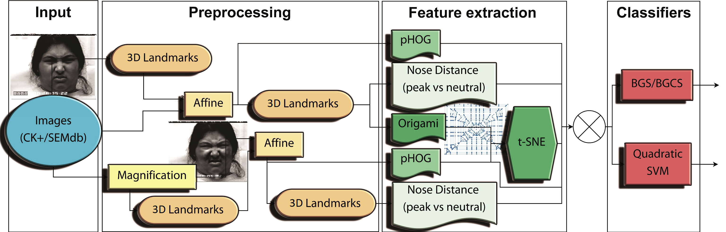
Figure 1: The diagram of the proposed methodology visualising the steps from input and preprocessing, to face representation and classification for all the suggested variations considering the classic feature based machine learning solutions.

Our proposed methodology comprises a data preprocessing, a face representation and a classification phase. These phases are applied both for feature based learning methods and deep architectures. Regarding the feature based methods (see figure 1), in the preprocessing phase, facial landmarks are extracted with or without Eulerian Video Magnification and an affine transform is applied for landmark and face alignment. In order to obtain subpixel alignment accuracy the locations are refined using frequency domain registration methods, [Argyriou and Vlachos, 2003, Argyriou and Vlachos, 2005, Argyriou, 2011]. In the face representation phase and the feature based learning approaches, a pyramid Histogram of Gradients (pHOG) descriptor is utilised. After the affine transformation new facial landmarks are extracted and they are used as input both to the Lang’s Universal Molecule algorithm to extract the novel origami descriptors and to the facial displacement descriptor (i.e., the Euclidean distance between the nose location in a neutral and a ‘peak’ frame representative of the expression). Finally, in the classification phase, the pHOG features are used as input to a Bayesian Compressed Sensing (BCS) and a Bayesian Group-Sparse Compressed Sensing (BGCS) classifiers, while the origami and nose-distance displacement descriptors are provided as inputs to a Quadratic Support Vector Machine (SVM) classifier. The t-Distributed Stochastic Neighbor Embedding (tSNE) dimensionality reduction technique is applied to the origami descriptor before the SVM classifier.

Regarding, the deep neural networks and considering an architecture based on the work on Attentional Recurrent Relational Network-LSTM (ARRN-LSTM) or the Spatial-Temporal Graph Convolutional Networks (ST-GCN) [Li et al., 2018, Yan et al., 2018], while the preprocessing stage remains the same. The input images are processed to extract facial landmarks, and then aligned. Furthermore, the process is applied twice and the second time for the motion magnified images. During the face representation the proposed origami representation is applied on the extracted landmarks and then the obtained pattern is imported to the above networks aiming to model simultaneously both spatial and temporal information. The utilised methodology is summarized in Figure 1 and the whole process is described in detail in the following subsections.

2.1 Preprocessing Phase

The two main techniques used in the data preprocessing phase (apart from the facial landmarks extraction) are the affine transform for landmark alignment and the Eulerian Video Magnification (EVM). In the preprocessing phase a set of output sequences are generated based on a combination of different techniques.

SEC-1: The first output comprises affine transformation of the original sequence of images which are then rescaled to 120$\times$120 pixels and converted to gray-scale. This represents the input of the pHOG descriptor.

SEC-2: The second output comprises Eulerian magnified images which are then affine transformed, rescaled to 120$\times$120 pixels and converted to gray scale. This represents again the input of the pHOG descriptor.

SEC-3: In the third output, the approaches proposed in [Kumar and Chellappa, 2018, Baltrusaitis et al., 2016, Argyriou and Petrou, 2009] are used before and after the affine transformation to reconstruct the face and obtain the 3D facial landmarks. This is provided as input to the facial displacement and the proposed origami descriptor.

SEC-4: In the fourth output, the facial landmarks are obtained from the Eulerian motion magnified images, the affine transform is applied and the facial landmarks are estimated again. This is given as input to the facial feature displacement descriptor.

The same process is considered for the deep ARRN-LSTM architecture with input the obtained 3D facial landmarks extracted by the proposed origami transformation.

2.2 Feature Extraction Phase

Three schemes have been used in this phase for the classic feature based learning approaches, (1) the pyramid Histogram of Gradients (pHOG), (2) a facial feature displacement descriptor, and (3) the proposed origami descriptor. These schemes are analysed below.

pHOG features extraction: The magnified affine transformed sequence (i.e., SEC-2) is provided as input to the pHOG descriptor. More specifically, eight bins on three pyramid levels of the pHOG are applied in order to obtain a row of $h_{m}$ features per sequence. For comparison purposes, the same process is applied to the unmagnified sequence (i.e., SEC-1) and a row of $h$ features per sequence is obtained respectively.

Facial feature displacement: The magnified facial landmarks (i.e., fourth sequence output of the preprocessing phase) are normalised according to a fiducial face point (i.e., nose) to account for head motion in the video stream. In other words, the nose is used as a reference point, such that the position of all the facial landmarks are independent of the location of the subject’s head in the images. If $L_{i}=[L_{i_{x}}\quad L_{i_{y}}]$ are the original image coordinates of the $i$-th landmark, and $L_{n}=[L_{n_{x}}\quad L_{n_{y}}]$ the nose landmark coordinates, the normalized coordinates are given by $l_{i}=[L_{i_{x}}-L_{n_{x}}\quad L_{i_{y}}-L_{n_{y}}]$.

The facial displacement features are the distances between each facial landmark in neutral pose and the corresponding ones in the ‘peak’ frame that represents the corresponding expression. The displacement of the $i$-th landmark (i.e., $i$-the vector element) is calculated using the Euclidean distance

$$d(l_{i}^{(p)},l_{i}^{(n)})=\sqrt{(l_{i_{x}}^{(p)}-l_{i_{x}}^{(n)})^{2}-(l_{i_{y}}^{(p)}-l_{i_{y}}^{(n)})^{2}}$$ (1)

between its normalised position in neutral frame ($l_{i}^{(n)}$) and the ‘peak’ frame ($l_{i}^{(p)}$). In the remaining of this paper, we will be referring to these features as distance to nose (neutral vs peak) features (DTNnp). The output of the DTNnp descriptor is a $d_{m}$ long row vector per sequence. For comparison purposes, the same process is applied to unmagnified facial landmark sequences (i.e., the third sequence of the preprocessing phase) and a row of $d$ features per sequence is obtained accordingly.

2.2.1 Origami based 3D face Representation

The origami representation is created from the normalised facial 3D landmarks (i.e., SEC-3). The descriptor is using $o$ facial landmarks in order to create an undirected graph of $n$ nodes and $e$ edges representing the facial crease pattern. The $n$ nodes contain the information of the $x$ and $y$ landmark coordinates, while the $e$ edges contain the IDs of the two nodes connected by the corresponding edge (which represent the nodes/landmarks relationships). The facial crease pattern creation process is divided into three main steps: shadow tree, Lang’s polygon and shrinking.

The first step implies the extraction of the flap projection of the face (shadow tree), from the facial landmarks. This shadow tree or metric tree $(T,d)$ is composed of leaves (external nodes) $N_{e}x={n_{1},...,n_{p}}$, internal nodes $N_{i}n={b_{1},...,b_{q}}$, edges $E$ and distances $d$ to the edges. This distance is the Euclidean distance between connected landmarks (nodes) through an edge in the tree. It is just a distance measured between each landmark that is going to be used during the Lang’s Polygon creation and during the shrinking step. The shadow tree is created as a linked version of 2D facial landmarks of the eyebrows, eyes, nose and mouth (see Figure 2).

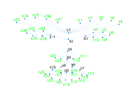
Figure 2: Shadow tree. The facial landmarks are linked creating a symmetric tree.

During the second step a convex doubling cycle polygon (Lang’s polygon) $L_{p}$, is created from the shadow tree $(T,d)$, based on the double cycling polygon $f$ creation algorithm. According to this process we are walking from one leaf node to the next one in the tree until reaching the initial node. Therefore, the path to go from $n_{1}$ to $n_{2}$ includes the path from $n_{1}$ to $b_{1}$ and from $b_{1}$ to $n_{2}$; the path from $n_{2}$ to $n_{3}$ also requires to pass through $b_{1}$; and the path from $n_{5}$ to $n_{6}$ goes through $b_{1}$, $b_{2}$ and $b_{3}$. In order to guaranty the resultant polygon to be convex, we shaped it as a rectangle (see Figure 3), where the top side contains the landmarks of the eyebrows, the sides are formed by the eyes and nose, and the mouth landmarks are at the bottom. This Lang’s polygon represents the area of the face that is going to be folded.

The obtained convex polygonal region has to satisfy the following condition: the distance between the leaf nodes $n_{i}$ and $n_{j}$ in the polygon ($d_{P}$) should be equal or greater than the distance of those leaf nodes in the shadow tree ($d_{T}$). This requirement is mainly due to the origami properties, so since a shadow tree come from a folded piece of paper (face), once it is unfolded to see the crease pattern, the distances on the unfolded paper $d_{P}(n_{i},n_{j})$ are going to be always larger or equal to the distances in the shadow tree $d_{T}(n_{i},n_{j})$.

$$d_{P}(n_{i},n_{j})\geq d_{T}(n_{i},n_{j})$$ (2)

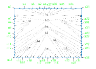
Figure 3: Based on Lang’s polygon rules, a rectangle-shaped initial convex doubling cycle polygon was created from the shadow tree in order to start with the same initial polygon shape for any face. The dashed arrows point the correspondent internal nodes $b_{i}$ and the straight arrows point the leave nodes $n_{i}$.

The third step corresponds to the shrinking process of this polygon. All the edges are moving simultaneously towards the centre of the polygon at constant speed until one of the following two events occur: contraction or splitting. The contraction event happens when the points collide in the same position (see Eq. 3). In this case, only one point is kept and the shrinking process continues (see Figure 4).

$$d_{P}(n_{i},n_{j})\leq th,\quad\textrm{then}\quad n_{i}=n_{j}$$ (3)

where $j=i+1$ and $th$ is a positive number $\approx 0$.

The splitting event occurs when the distance between two non-consecutive points is equal to their shadow tree distance (see Figure 5).

$$d_{P}(n_{i},n_{k})\leq d_{T}(n_{i},n_{k})+th$$ (4)

where $k\geq i+1$ and $th$ is a positive number $\approx 0$. As a consequence of this event a new edge is generated between these points creating two new sub-polygons. The shrinking process continues on each polygon separately.

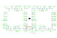
Figure 4: Contraction event. In this case the distance between nodes 24 and 25 is 0 so one of the nodes is eliminated. Therefore the number of leaf nodes is reduced to 36. Nodes 13 and 14 are close but not close enough to trigger a contraction event.

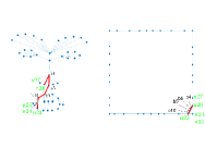
Figure 5: Splitting event. When the distance between two non-consecutive points in Lang’s polygon (nodes 23 and 26) is the same as the distance of those two points in the shadow tree, a new edge is created. The intermediate nodes in the tree are also located in the new edge (nodes b4, b5, b9, b10).

Finally, the process will end when all the points converge, creating a crease pattern, $C=g(f({T,d}))$, where $(T,d)$ is the shadow tree, $f(T,d)$ is the Lang polygon, $C$ is the crease pattern and $g$ and $f$ are the processes to create the double cycle polygon and shrinking functions, respectively. Due to the structure of our initial Lang’s polygon, the final crease patterns will have a structure similar to the one shown in Figure 6.

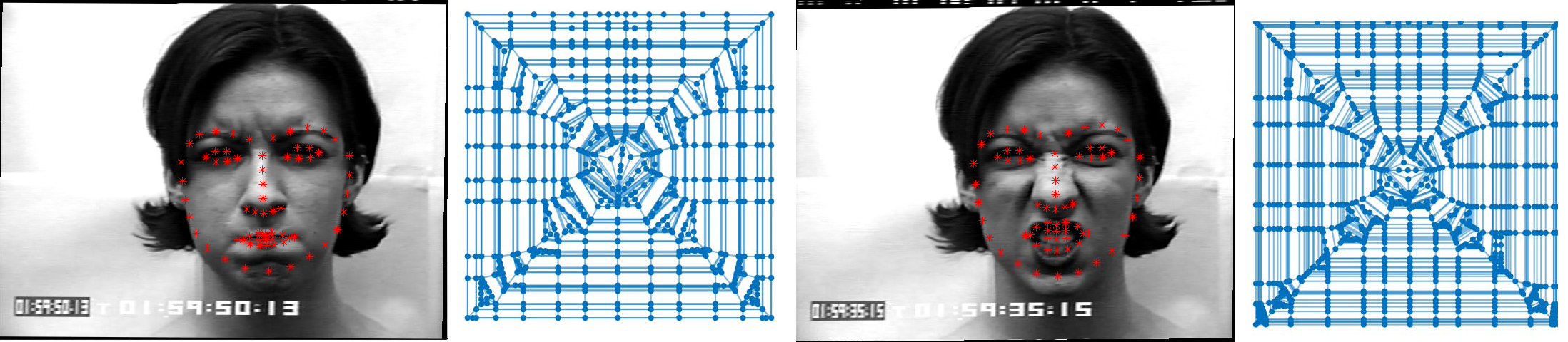
Figure 6: This image shows the crease pattern from the proposed algorithm applied to our rectangular convex doubling cycle polygon produced from the facial landmarks.

The crease pattern is stored as an undirected graph containing the coordinates of each node and the required information for the edges (i.e. IDs of linked nodes). Due to the fact that $x$ and $y$ coordinates and the linked nodes are treated as vectorial features, these can be represented more precisely by a complex or hyper-complex representation, as shown in [Adali et al., 2011]. A vector can be decomposed into linearly independent components, in the sense that they can be combined linearly to reconstruct the original vector. However, depending on the phenomenon that changes the vector, correlation between the components may exist from a statistical point of view (i.e. two uncorrelated variables are linearly independent but two linearly independent variables are not always uncorrelated). If they are independent our proposed descriptor does not provide any significant advantage, but if there is correlation this is considered. In most of the cases during the feature extraction process complex or hyper-complex features are generated but decomposed to be computed by a classifier [Adali et al., 2011, Li et al., 2011]. In our case, the coordinates of the nodes are correlated and also the node IDs that represent the edges. Therefore, the nodes and edges are represented as show in 5 and 6.

$$n={n_{i}}_{x}+i\textperiodcentered{n_{i}}_{y}$$ (5)

$$e={{e_{i}}\_nodeID_{1}+i\textperiodcentered{e_{i}}\_nodeID_{2}}$$ (6)

where ${n_{i}}_{x}$ and ${n_{i}}_{y}$ is the coordinate $x$ and $y$ of the $i_{t}h$ leave node; and ${e_{i}}\_nodeID_{1}$ and ${e_{i}}\_nodeID_{2}$ are the identifiers of the nodes linked by the $ith$ edge.

2.3 Classification Phase

2.3.1 Feature based classification approaches

Two state-of-the-art methods have been used in the third and last phase of the proposed emotion classification approach. The first method is based on a Bayesian Compressed Sensing (BCS) classifier, including its improved version for Action Units detection, and a Bayesian Group-Sparse Compressed Sensing (BGCS) classifier, similar to the one presented in [Song et al., 2015]. The second method is similar to [Michel and Kaliouby, 2003] and is based on a quadratic SVM classifier which has been successfully applied for emotion classification in [Buciu and Pitas, 2003].

3 RESULTS

Data from two different datasets (CK+ and SEMdb) is used to validate the classification performance of the methods by calculating the classification accuracy and the F1 score. The CK+ dataset contains 593 sequences of images from 123 subjects. Each sequence starts with a neutral face and ends with the peak stage of an emotion. The CK+ contains AU labels for all of them but basic emotion labels only for 327. The SEMdb contains 810 recordings from 9 subjects. The start of each recording is considered as a neutral face and the peak frame is the one whose landmarks vary most from the respective landmarks in the neutral face. SEMdb contains labels for 4 classes related to autobiographical memories. These autobiographical memory classes are represented by spontaneous facial micro-expressions triggered by the observation of 4 different stimulations related to distant and recent autobiographical memories.

The next paragraphs explain the obtained results ordered by the objective classes (AUs, 7 basic emotions or 4 autobiographical emotions). The experiments are compared with results obtained using two state of the art methods: Bayesian Group-Sparse Compressed Sensing [Song et al., 2015] and landmarks to nose [Michel and Kaliouby, 2003]. Song et al. method compares two classification algorithms, i.e., the Bayesian Compressed Sensing (BCS) and their proposed improvement Bayesian Group-Sparse Compressed Sensing (BGCS). Both classifiers are used to detect 24 Action Units within the CK+ dataset using pHOG features. Landmarks to nose methods consist on using the landmarks distance to nose difference between the peak and neutral frame as input of an SVM classifier to classify 7 basic emotions in  [Michel and Kaliouby, 2003] or 4 autobiographical emotions in [Montenegro et al., 2016]. Regarding the DNN architectures the comparative study is performed with the original method proposed by Yan in [Yan et al., 2018] considering both the origami graph in a Graph Convolutional network with and without Eulerian Video Magnification.

The 24 AUs detection experiment involved the BCS and the BGCS classifiers and CK+ database. The input features utilised included the state of the art ones and them combined with our proposed ones. Therefore, for the AUs experiment the pHOG were tested independently and combined with the proposed magnified pHOG and origami features; and identically with the distance to nose features. The result of the different combinations are shown in Figure 7, Table 1 and Table 2. They show that the contribution of the new descriptors improves the F1 score and the overall accuracy.

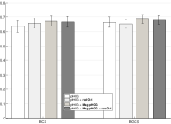
Figure 7: F1 score results of the 24 AUs classification using the state of the art methods BCS and BGCS and the new results when the novel features are added.

Table 1: Mean of k-fold F1 score and Accuracy values. 24 AU from CK+ dataset are classified using 4 combinations of features and BCS and BGCS classifier

Method	Meas.	Features
		pHOG	pHOG	pHOG	pHOG
			Ori	Mag pHOG	Mag pHOG
					red Ori
BCS	F1	0.636	0.658	0.673	0.667
	ACC	0.901	0.909	0.909	0.912
BGCS	F1	0.664	0.654	0.687	0.679
	ACC	0.906	0.908	0.913	0.91

Table 2: Mean of k-fold F1 score and Accuracy values. 24 Action Units from CK+ dataset are classified. A combination of the DTNnp [Montenegro et al., 2016], the pHOG [Song et al., 2015] extracted from the magnified version of the data and the novel origami features are used as input to the BCS/BGCS classifiers.

Method	Meas.	Features
		DTNnp	DTNnp	DTNnp
			Mag pHOG	Mag pHOG
				Ori
BCS	F1	0.407	0.671	0.663
	ACC	0.873	0.913	0.914
BGCS	F1	0.555	0.69	0.682
	ACC	0.893	0.915	0.914

The second experiment’s objective was the classification of 7 basic emotions using a quadratic SVM classifier, the distance to nose features combined with the proposed ones and the CK+ database. The results shown in Table 3 the quadratic SVM ones. The combination of the features did not provide any noticeable boost in the accuracy. The increment in the F1 score is not big enough to be taken into account. Similar results were obtained for the VGG-S architecture with an increment in accuracy and the F1 score.

Table 3: Mean of k-fold F1 score and Accuracy values. 7 emotion classes from CK+ dataset are classified. A combination of the DTNnp [Montenegro et al., 2016], the pHOG [Song et al., 2015] extracted from the magnified version of the data and the novel origami features are used as input to the quadratic SVM classifier. The final rows demonstrate the results obtained using the VVG-S architectures.

Method	Meas.	Features
		DTNnp	DTNnp	DTNnp
			Mag pHOG	Mag pHOG
				Ori
qSVM	F1	0.861	0.857	0.865
	ACC	0.899	0.893	0.899
Method	Meas.	Orig	Origami	Origami + Mag
VGG-S	F1	0.269	0.282	0.284
	ACC	0.24	0.253	0.26

Table 4: The obtained confusion matrix for the 7 emotions present in the CK+ dataset.

	anger	cont	disg	fear	happy	sadn	surpr
anger	38	2	3	0	0	2	0
contempt	1	15	0	0	1	1	0
disgust	5	0	54	0	0	0	0
fear	0	0	0	19	4	0	2
happy	0	2	0	1	66	0	0
sadness	3	0	1	1	1	22	0
surprise	0	2	0	0	1	0	80

Table 4 shows the confusion matrix of the emotions classified for the best F1 score experiments. This confusion matrix shows that fear is the emotion with less rate of success and surprise and happiness to be the more accurately recognised. The third experiment involved the BCS and quadratic SVM classifiers, using the SEMdb dataset, pHOG features and a combination of pHOG and distance to nose features (both combined with the proposed ones) and detecting the corresponding 4 classes that are related to autobiographical memories. Both classifiers (BCS and SVM) provide improved classification estimates when the combination of all features is used to detect the 4 autobiographical memory classes.

4 CONCLUSION

We presented the improvement that novel preprocessing techniques and novel representations can provide in the classification of emotions from facial images or videos. Our study proposes the use of Eulerian magnification in the preprocessing stage and an origami algorithm in the feature extraction stage. Our results show that the addition of these techniques can help to increase the overall classification accuracy both for Graph Convolutional Network and feature based methods.

REFERENCES

- Abadia et al., 2015 Abadia, M. K., Subramanian, R., Kia, S. M., Avesani, P., Patras, I., and Sebe, N. (2015). Decaf: Meg-based multimodal database for decoding affective physiological responses. IEEE Transactions on Affective Computing, 6(3):209–222.
- Adali et al., 2011 Adali, T., Schreier, P., and Scharf, L. (2011). Complex-valued signal processing: The proper way to deal with impropriety. IEEE Transactions on Signal Processing, 59(11):5101–5125.
- Alpher, 2015 Alpher, A. (2015). Automatic analysis of facial affect: A survey of registration, representation, and recognition. IEEE transactions on pattern analysis and machine intelligence, 37(6):1113–1133.
- Argyriou, 2011 Argyriou, V. (2011). Sub-hexagonal phase correlation for motion estimation. IEEE Transactions on Image Processing, 20(1):110–120.
- Argyriou and Petrou, 2009 Argyriou, V. and Petrou, M. (2009). Chapter 1 photometric stereo: An overview. In Hawkes, P. W., editor, Advances in IMAGING AND ELECTRON PHYSICS, volume 156 of Advances in Imaging and Electron Physics, pages 1 – 54. Elsevier.
- Argyriou and Vlachos, 2003 Argyriou, V. and Vlachos, T. (2003). Sub-pixel motion estimation using gradient cross-correlation. In Seventh International Symposium on Signal Processing and Its Applications, 2003. Proceedings., volume 2, pages 215–218 vol.2.
- Argyriou and Vlachos, 2005 Argyriou, V. and Vlachos, T. (2005). Performance study of gradient correlation for sub-pixel motion estimation in the frequency domain. IEE Proceedings - Vision, Image and Signal Processing, 152(1):107–114.
- Baltrusaitis et al., 2016 Baltrusaitis, T., Robinson, P., and Morency, L. P. (2016). Openface: an open source facial behavior analysis toolkit. IEEE Winter Conference on Applications of Computer Vision (WACV), pages 1–10.
- Bettadapura, 2012 Bettadapura, V. (2012). Face expression recognition and analysis: the state of the art. Tech Report arXiv:1203.6722, pages 1–27.
- Bowers and Streinu, 2015 Bowers, J. C. and Streinu, I. (2015). Lang’s universal molecule algorithm. Annals of Mathematics and Artificial Intelligence, 74(3–4):371–400.
- Buciu and Pitas, 2003 Buciu, I. and Pitas, I. (2003). Ica and gabor representation for facial expression recognition. ICIP, 2:II–855.
- Chowdhuri and Bojewar, 2016 Chowdhuri, M. A. D. and Bojewar, S. (2016). Emotion detection analysis through tone of user: A survey. International Journal of Advanced Research in Computer and Communication Engineering, 5(5):859–861.
- Chu et al., 2017 Chu, W., la Torre, F. D., and Cohn, J. (2017). Learning spatial and temporal cues for multi-label facial action unit detection. Autom Face and Gesture Conf, 4.
- Corneanu et al., 2016 Corneanu, C., Simon, M., Cohn, J., and Guerrero, S. (2016). Survey on rgb, 3d, thermal, and multimodal approaches for facial expression recognition: History, trends, and affect-related applications. IEEE transactions on pattern analysis and machine intelligence, 38(8):1548–1568.
- den Stock et al., 2015 den Stock, J. V., Winter, F. D., de Gelder, B., Rangarajan, J., Cypers, G., Maes, F., Sunaert, S., and et. al. (2015). Impaired recognition of body expressions in the behavioral variant of frontotemporal dementia. Neuropsychologia, 75:496–504.
- Ekman and Friesen, 1978 Ekman, P. and Friesen, W. (1978). The facial action coding system: A technique for the measurement of facial movement. Consulting Psychologists.
- Gudi et al., 2015 Gudi, A., Tasli, H., den Uyl, T., and Maroulis, A. (2015). Deep learning based facs action unit occurrence and intensity estimation. In Automatic Face and Gesture Recognition (FG), 2015 11th IEEE International Conference and Workshops on, 6:1–5.
- Izard, 2013 Izard, C. E. (2013). Human emotions. Springer Science and Business Media.
- Kanade et al., 2000 Kanade, T., Cohn, J. F., and Tian, Y. (2000). Comprehensive database for facial expression analysis. Fourth IEEE International Conference on Automatic Face and Gesture Recognition, pages 46–53.
- Kumar and Chellappa, 2018 Kumar, A. and Chellappa, R. (2018). Disentangling 3d pose in a dendritic cnn for unconstrained 2d face alignment.
- Lang, 1996 Lang, R. J. (1996). A computational algorithm for origami design. In Proceedings of the twelfth annual symposium on Computational geometry, pages 98–105.
- Li et al., 2018 Li, L., Zheng, W., Zhang, Z., Huang, Y., and Wang, L. (2018). Skeleton-based relational modeling for action recognition. CoRR, abs/1805.02556.
- Li et al., 2011 Li, X., Adali, T., and Anderson, M. (2011). Noncircular principal component analysis and its application to model selection. IEEE Transactions on Signal Processing, 59(10):4516–4528.
- Lokannavar et al., 2015a Lokannavar, S., Lahane, P., Gangurde, A., and Chidre, P. (2015a). Emotion recognition using eeg signals. International Journal of Advanced Research in Computer and Communication Engineering, 4(5):54–56.
- Lokannavar et al., 2015b Lokannavar, S., Lahane, P., Gangurde, A., and Chidre, P. (2015b). Emotion recognition using eeg signals. Emotion, 4(5):54–56.
- Lucey et al., 2010 Lucey, P., Cohn, J., Kanade, T., Saragih, J., Ambadar, Z., and Matthews, I. (2010). The extended cohn-kanade dataset (ck+): A complete dataset for action unit and emotion-specified expression. In Computer Vision and Pattern Recognition Workshops (CVPRW), 2010 IEEE Computer Society Conference on, pages 94–101.
- McKeown et al., 2012 McKeown, G., Valstar, M., Cowie, R., Pantic, M., and Schroder, M. (2012). The semaine database: Annotated multimodal records of emotionally colored conversations between a person and a limited agent. IEEE Transactions on Affective Computing, 3(1):5–17.
- Michel and Kaliouby, 2003 Michel, P. and Kaliouby, R. E. (2003). Real time facial expression recognition in video using support vector machines. In Proceedings of the 5th international conference on Multimodal interfaces, pages 258–264.
- Montenegro et al., 2016 Montenegro, J., Gkelias, A., and Argyriou, V. (2016). Emotion understanding using multimodal information based on autobiographical memories for alzheimer’s patients. ACCVW, pages 252–268.
- Montenegro and Argyriou, 2017 Montenegro, J. M. F. and Argyriou, V. (2017). Cognitive evaluation for the diagnosis of alzheimer’s disease based on turing test and virtual environments. Physiology and Behavior, 173:42 – 51.
- Ngo et al., 2016 Ngo, A. L., Oh, Y., Phan, R., and See, J. (2016). Eulerian emotion magnification for subtle expression recognition. ICASSP, pages 1243–1247.
- Nicolaou et al., 2011 Nicolaou, M. A., Gunes, H., and Pantic, M. (2011). Continuous prediction of spontaneous affect from multiple cues and modalities in valence-arousal space. IEEE Transactions on Affective Computing, 2(2):92–105.
- Nicolle et al., 2012 Nicolle, J., Rapp, V., Bailly, K., Prevost, L., and Chetouani, M. (2012). Robust continuous prediction of human emotions using multiscale dynamic cues. 14th ACM conf on Multimodal interaction, pages 501–508.
- Pantic et al., 2005 Pantic, M., Valstar, M., Rademaker, R., and Maat, L. (2005). Web-based database for facial expression analysis. IEEE international conference on multimedia and Expo, pages 317–321.
- Park et al., 2015 Park, S., Lee, S., and Ro, Y. (2015). Subtle facial expression recognition using adaptive magnification of discriminative facial motion. 23rd ACM international conference on Multimedia, pages 911–914.
- Sariyanidi et al., 2013 Sariyanidi, E., Gunes, H., Gkmen, M., and Cavallaro, A. (2013). Local zernike moment representation for facial affect recognition. British Machine Vision Conf.
- Soleymani et al., 2016 Soleymani, M., Asghari-Esfeden, S., Fu, Y., and Pantic, M. (2016). Analysis of eeg signals and facial expressions for continuous emotion detection. IEEE Transactions on Affective Computing, 7(1):17–28.
- Soleymani et al., 2012 Soleymani, M., Lichtenauer, J., Pun, T., and Pantic, M. (2012). A multimodal database for affect recognition and implicit tagging. IEEE Transactions on Affective Computing, 3(1):42–55.
- Song et al., 2015 Song, Y., McDuff, D., Vasisht, D., and Kapoor, A. (2015). Exploiting sparsity and co-occurrence structure for action unit recognition. In Automatic Face and Gesture Recognition (FG), 2015 11th IEEE International Conference and Workshops on, 1:1–8.
- Valstar et al., 2017 Valstar, M., Sánchez-Lozano, E., Cohn, J., Jeni, L., Girard, J., Zhang, Z., Yin, L., and Pantic, M. (2017). Fera 2017: Addressing head pose in the third facial expression recognition and analysis challenge. arXiv preprint arXiv:1702.04174, 19(1-–12):888–896.
- Wadhwa et al., 2016 Wadhwa, N., Wu, H., Davis, A., Rubinstein, M., Shih, E., Mysore, G., Chen, J., Buyukozturk, O., Guttag, J., Freeman, W., and Durand, F. (2016). Eulerian video magnification and analysis. Communications of the ACM, 60(1):87–95.
- Weninger et al., 2015 Weninger, F., Wllmer, M., and Schuller, B. (2015). Emotion recognition in naturalistic speech and language survey. Emotion Recognition: A Pattern Analysis Approach, pages 237–267.
- Wu et al., 2012 Wu, H., Rubinstein, M., Shih, E., Guttag, J., Durand, F., and Freeman, W. (2012). Eulerian video magnification for revealing subtle changes in the world. ACM Transactions on Graphics, 31:1–8.
- Yan, 2017 Yan, H. (2017). Collaborative discriminative multi-metric learning for facial expression recognition in video. Pattern Recognition.
- Yan et al., 2018 Yan, S., Xiong, Y., and Lin, D. (2018). Spatial temporal graph convolutional networks for skeleton-based action recognition. CoRR, abs/1801.07455.
- Yan et al., 2014 Yan, W. J., Li, X., Wang, S. J., Zhao, G., Liu, Y. J., Chen, Y. H., and Fu, X. (2014). Casme ii: An improved spontaneous micro-expression database and the baseline evaluation. PloS one, 9(1):e86041.
- Yi et al., 2013 Yi, J., Mao, X., Xue, Y., and Compare, A. (2013). Facial expression recognition based on t-sne and adaboostm2. GreenCom, pages 1744–1749.
- Zeng et al., 2009 Zeng, Z., Pantic, M., Roisman, G. I., and Huang, T. S. (2009). A survey of affect recognition methods: Audio, visual, and spontaneous expressions. PAMI, 31(1):39–58.
- Zhao and Pietikinen, 2009 Zhao, G. and Pietikinen, M. (2009). Boosted multi-resolution spatiotemporal descriptors for facial expression recognition. Pattern recognition letters, 30(12):1117–1127.