Localized inverse factorizationE. H. Rubensson, A. G. Artemov, A. Kruchinina, and E. Rudberg
Localized inverse factorization††thanks: \fundingThis work was supported by the Swedish research council under grant 621-2012-3861 and the Swedish national strategic e-science research program (eSSENCE).
Abstract
We propose a localized divide and conquer algorithm for inverse factorization of Hermitian positive definite matrices with localized structure, e.g. exponential decay with respect to some given distance function on the index set of . The algorithm is a reformulation of recursive inverse factorization [J. Chem. Phys., 128 (2008), 104105] but makes use of localized operations only. At each level of recursion, the problem is cut into two subproblems and their solutions are combined using iterative refinement [Phys. Rev. B, 70 (2004), 193102] to give a solution to the original problem. The two subproblems can be solved in parallel without any communication and, using the localized formulation, the cost of combining their results is proportional to the cut size, defined by the binary partition of the index set. This means that for cut sizes increasing as with system size the cost of combining the two subproblems is negligible compared to the overall cost for sufficiently large systems.
We also present an alternative derivation of iterative refinement based on a sign matrix formulation, analyze the stability, and propose a parameterless stopping criterion. We present bounds for the initial factorization error and the number of iterations in terms of the condition number of when the starting guess is given by the solution of the two subproblems in the binary recursion. These bounds are used in theoretical results for the decay properties of the involved matrices.
The localization properties of our algorithms are demonstrated for matrices corresponding to nearest neighbor overlap on one-, two-, and three-dimensional lattices as well as basis set overlap matrices generated using the Hartree–Fock and Kohn–Sham density functional theory electronic structure program Ergo [SoftwareX, 7 (2018), 107].
1 Introduction
A standard approach to the solution of generalized eigenproblems
| (1) |
where and are Hermitian and is positive definite, makes use of an inverse factor of to transform the eigenvalue problem to standard form [27, 28]. If we have that
| (2) |
then (1) implies
| (3) |
Inverse factors may also be used in the solution of linear systems, either as part of a direct solver or as approximate inverse preconditioners for iterative solvers. We are here motivated by the solution of the self-consistent field equations appearing in a number of electronic structure models such as Hartree–Fock and Kohn–Sham density functional theory. In this context, is the Fock/Kohn–Sham matrix and the density matrix is given by a subset of the eigenvectors of (1) as
| (4) |
where nocc is the number of occupied electron orbitals and the eigenvalues are ordered in ascending order, . The corresponding density matrix for the standard problem (3) is given by
| (5) |
which is related to (4) by . In self-consistent field calculations, is the basis set overlap matrix, in other contexts referred to as the mass or Gram matrix. Some of the most efficient methods to compute the density matrix assume the eigenproblem is on standard form [20, 32, 36, 43, 48]. Unless (corresponding to an orthogonal basis) the computation of the density matrix then consists of three steps [42]:
A simple and efficient method for the second step sees the problem as a matrix function where is the Heaviside function and and uses a polynomial expansion in to compute . The computational kernel is matrix-matrix multiplication for which implementations achieving good performance usually exist regardless of computational platform. For systems with nonvanishing eigenvalue gap at and local basis sets, the computational complexity with respect to system size can be reduced to linear, , with control of the forward error [41]. The foundation for linear scaling methods has been discussed extensively in the literature, see e.g. [1, 9, 21, 22]. Of particular importance are the decay properties of the density matrix [1] that are the basis of sparse approximations where only matrix entries are stored [25, 29, 38]. Here we note that to take advantage of the decay properties in the three-step approach outlined above, an inverse factor that allows for a sparse approximation with entries must be used.
There is an infinite number of matrices that are inverse factors of , i.e. that fulfill . The ones most commonly used are the inverse square root (Löwdin) [17, 26, 49] and inverse Cholesky factors [7, 40], both of which have the important property of decay of matrix element magnitude with atomic separation [1]. The cost of standard methods for their computation in general scales cubically with system size. A linearly scaling alternative is based on iterative refinement [33] which, given a starting guess , produces a sequence of matrices with convergence to an inverse factor of if the initial factorization error
| (6) |
The iterative refinement converges to the inverse square root if commutes with and to some other inverse factor otherwise. The starting guess is often set to the identity matrix, scaled so that (6) is fulfilled [17, 49]. Being based on matrix-matrix multiplication the iterative refinement approach has advantages similar to those of the recursive density matrix expansions for the second step in the three-step approach described above.
Recursive inverse factorization, considered in the present work, also makes use of iterative refinement but does so in a hierarchical manner [37]. A binary partition of the index set of is applied corresponding to a binary principal submatrix decomposition
| (7) |
inverse factors and of and , respectively, are computed and
| (8) |
is used as starting guess for iterative refinement. This binary partitioning is applied recursively which gives the recursive inverse factorization method. The initial factorization error depends on the binary partition of the index set and one may thus attempt to partition the index set so that the initial error becomes as small as possible. It was shown in [37] that any binary partition or cut of the index set in two pieces leads to (6) being fulfilled. The index set may for example correspond to the vertices of a graph or centers of atom-centered basis functions. In this article, the terms vertex and index are used interchangeably.
In the present work, we further analyze the recursive inverse factorization method and propose a localized version. This variant exhibits more localized computations and is even more amenable to parallelization. Under certain assumptions, including being localized with respect to some given distance function on its index set and provided that matrix entries with magnitude below some fixed threshold value are discarded, we show that using this localized inverse factorization the workload for the iterative refinement used to glue together and is proportional to the cut size. Thus, provided that a principal submatrix cut can be done so that only a small number of vertices, e.g. , are close to the cut, the cost of the iterative refinement is negligible compared to the inverse factorizations of and for sufficiently large systems, e.g. versus . In case is the overlap matrix for a local atom-centered basis set, the distance function may, with our formulation of localization, be taken as the Euclidean distance between basis function centers. In this case it is usually straightforward to make a binary division such that only vertices are close to the cut. The two subproblems to compute inverse factors of and are completely disconnected and thus embarrassingly parallel.
In Section 2 we propose a sign matrix formulation for inverse factorization. This formulation is in Section 3 used in an alternative derivation of iterative refinement, making the relation to sign matrix and density matrix expansion methods evident. The stability of both regular and localized iterative refinement is considered and new stopping criteria are proposed. In Section 4 we introduce the binary principal submatrix decomposition and regular and localized iterative refinement algorithms including starting guesses given by the binary principal submatrix decomposition. We also derive convergence results, giving a bound for the number of iterative refinement iterations. In Section 5 we introduce the notion of exponential decay with respect to distance between vertices and exponential decay away from the cut. We derive localization results for the matrices occurring in regular and localized iterative refinement. In Section 6 we present the full recursive and localized inverse factorization algorithms. In Section 7 we present numerical experiments to demonstrate the localization properties of the recursive and localized inverse factorization algorithms. We end the article with concluding remarks in Section 8.
2 Inverse factorization from a sign matrix formulation
We present here a sign matrix formulation that we will use to derive methods for the iterative refinement of inverse factors.
Theorem 2.1.
Let be a Hermitian positive definite matrix and assume that is a nonsingular matrix. Then,
| (9) |
where and .
Proof 2.2.
Let
| (10) |
Since congruence transformation preserves positive definiteness, see e.g. [16, Theorem 4.5.8], is positive definite. The matrices and have the same eigenvalues since implies with . Therefore,
| (11) |
is positive definite, has no eigenvalues on the imaginary axis, and sign is defined. Eq. (9) with follows directly from and and follows from .
The special case of Theorem 2.1 with leading to was shown by Higham [12]. This special case already shows that methods for the matrix sign function can be used to compute the square root together with its inverse. Theorem 2.1 can be used to reduce the computational cost of the matrix sign function evaluation if an approximate inverse factor is available or can be cheaply obtained. This approximate inverse could be such that the condition number of the problem is reduced and/or such that only a local portion of the inverse factor needs to be updated. In general, will not be the inverse square root. However, if is Hermitian and commutes with , then and are simultaneously diagonalizable, i.e. and with unitary and diagonal , and
| (12) | ||||
| (13) |
Theorem 2.1 is closely related to and can be shown using [14, Lemma 4.3]. We note that may be computed using some method for the inverse square root applied to followed by multiplication with from the left. We note also that the eigenvalues of are real and given as positive-negative pairs .
3 Iterative refinement from sign matrix methods
Based on the sign matrix formulation above we provide here an alternative derivation of the iterative refinement method of [33]. The second order refinement can be derived from the Newton–Schulz sign function iteration [13]
| (14) |
with
| (15) |
This gives the iteration
| (16) |
The structure of is preserved and therefore only a single channel is needed for the iteration:
| (17) |
Higher order polynomial iterations can be derived using the condition that the polynomial has fixed points and a number of vanishing derivatives at and . These can be written as
| (18) |
where
| (19) |
and . The sign matrix residual is in each iteration reduced as
| (20) |
where
| (21) |
This leads to the iterative refinement
| (22) |
with a reduction of the error
| (23) |
where
| (24) |
is the factorization error in iteration . Note that (17) is the special case of (22) with . We have that and therefore the iterative refinement converges if . This also means that
| (25) |
and that an accuracy is reached within
| (26) |
iterations.
An alternative to (17) is given by applying the Newton–Schulz iteration with
| (27) |
which gives a coupled or dual channel iteration
| (28) |
This iteration has previously been considered with . Since commutes with , and then converges to the matrix square root and its inverse, respectively, as explained in the previous section. The corresponding higher order iterations can be obtained by inserting (27) in (18). This alternative is not further pursued in this work. We note that in the present context where the inverse factor does not have to be the inverse square root a drawback of (28) compared to (17) is that any accuracy lost during the iterations cannot be recovered. The polynomials in (18) can be seen as special cases of the Padé recursions for the matrix sign function [18]. Other Padé recursions may also be used in the present context but are not further considered in this article. We note also that the Newton-Schulz iteration in (14) is equivalent to the McWeeny polynomial [30] that has been frequently used in computations of the density matrix. Similarly, the higher order polynomials in (18) correspond to the higher order Holas polynomials [15]. Other alternatives not further pursued in this work includes the use of nonsymmetric polynomials in the expansion as in for example the SP2 algorithm for the density matrix [32] and the use of scaling techniques to reduce the number of iterations [19, 36].
3.1 Local refinement
If only a local correction to the approximate inverse factor is needed the cost of the iterative refinement can be reduced. Assuming that has non-negligible elements its computation using (24) will for large systems involve the computation of many matrix elements that are negligibly small. The factorization error can be written
| (29) |
as was noted in [37], or as an update to the previous step factorization error
| (30) |
which gives a dual channel iteration
| (31) |
In practice, the iteration is evaluated as
| (32) |
where the soft brackets indicate the order of evaluation. Iteration (32) is a key component of the localized inverse factorization proposed in this work. Its localization properties will be discussed later in this article.
3.2 Stability
If were assumed to be Hermitian and to commute with and exact arithmetics were used the order of the matrices in the matrix products of (17) and (22) would be arbitrary. In practice numerical errors cause loss of commutativity which for some iterations results in instabilities leading to unbounded growth of errors. This effect has been studied in several papers for different variants of (17) and for other matrix iterations. For example, the iterations
| (33) |
and
| (34) |
considered in for example [17, 34] and [6, 35], respectively, are both equivalent to (17) in exact arithmetics. However, both (33) and (34) are unstable unless is extremely well conditioned [6, 34]. Iteration (17) has been shown to be locally stable around [17]. Here we will first consider the stability of (22) around any inverse factor and for any . Then we will consider the stability of the local refinement given by (31).
Given a matrix function , the Fréchet derivative at in direction is a mapping, linear in , satisfying
| (35) |
for all [13]. We follow [8, 13, 14] and define a matrix iteration to be stable in a neighborhood of a fixed point if exists at and there is a constant such that for any . Here, the th power is used to denote p-fold composition of the Fréchet derivative in the second argument, e.g. .
Let
| (36) |
be the mapping associated with (22). We note that although implies , the converse is in general not true. For example, if , then both and with are fixed points of , but . Let . Then the Fréchet derivative at ,
| (37) |
is idempotent, i.e. , and thus has bounded powers.
Let
| (38) |
be the mapping associated with (31). Let . Then the Fréchet derivative at in direction
| (39) |
and
| (40) |
We have that is idempotent if is Hermitian. Thus, (31) is stable if non-Hermitian perturbations of are disallowed, which can simply be achieved by storing only the upper triangle of .
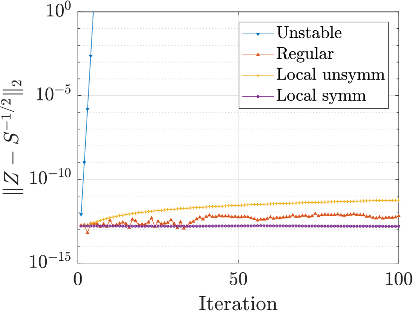
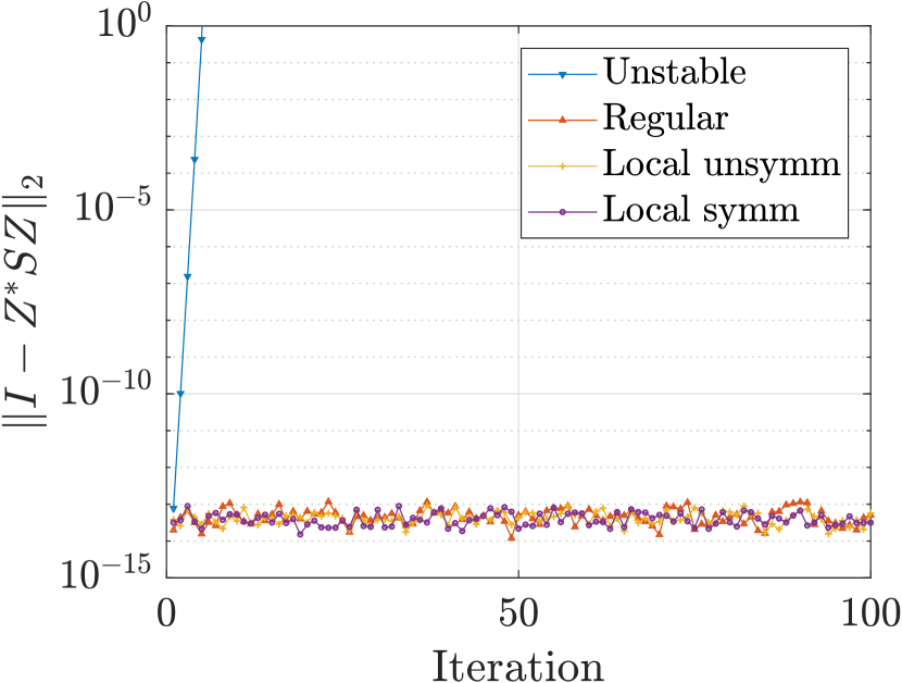
The stability properties of the matrix iterations above are demonstrated in Figure 1. Again, we follow [13] and apply the iterations to the Wilson matrix
| (41) |
For the local refinement without symmetric storage of , an unsymmetric perturbation in causes a small drift away from the initial inverse factor. However, the factorization error stays small.
3.3 Stopping criterion
Recently we proposed a new type of parameterless stopping criteria for iterative methods [24]. These stopping criteria were originally used in recursive polynomial expansions to compute the density matrix. The stopping criteria are based on the detection of a discrepancy between theoretical and observed orders of convergence, which takes place when numerical errors start to dominate the calculation. In other words, given some error measure or residual, the theoretical worst case reduction of the error is derived. If the error decreases any slower than this theoretical worst case reduction the calculation has reached the stagnation phase, and it is time to stop the iterations.
For the iterative refinement (22) a worst case error reduction is given by (25). We may therefore formulate our stopping criterion for the iterative refinement as stop as soon as .
3.3.1 Frobenius norm
The spectral norm can be expensive to compute in practical calculations. In particular, near the iterative refinement convergence the eigenvalues of may be clustered near 0, making it difficult for an iterative eigensolver to compute the spectral norm. One may therefore want to use a cheaper alternative in the stopping criterion. The computational cost of the Frobenius norm is independent of the eigenvalue distribution and requires just one pass over the matrix entries. The Frobenius norm is equal to
| (42) |
where are the eigenvalues of ordered so that for all .
Since , we have that for some . Following the discussion in [24] we have that if
| (43) |
then in exact arithmetics, using (25), we have that
| (44) |
and the stopping criterion for the iterative refinement can be formulated as stop as soon as .
Now we will show that the condition (43) is fulfilled. Let . Then, and we have
| (45) |
Moreover, the spectral norm can be written as
| (46) |
Then, we obtain
| (47) |
4 Binary principal submatrix decomposition
The basic component of our recursive and localized inverse factorization algorithms is a binary principal submatrix decomposition of . Let be partitioned as
| (48) |
and let and be inverse factorizations of and , respectively. Then, an inverse factor of can be computed using iterative refinement with
| (49) |
as starting guess, as described by Algorithm 1. To be able to strictly bound the number of iterations in exact arithmetics, we let Algorithm 1 not make use of the parameterless stopping criterion which relies on numerical errors to decide when to stop. In practical calculations, the parameterless stopping criterion is preferable and will be used in the formulation of the full recursive and localized algorithms in Section 6.
Algorithm 1 as is already features localized computations. The foregoing computation of and can be performed as two separate computations without any interaction or communication between them. The following iterative refinement employs matrix-matrix multiplications for which implementations with good performance usually exist, both for serial and parallel execution. Furthermore, the matrices involved in the algorithm are typically sparse with localized nonzero structure. If the sparse matrix-matrix multiplications are performed using the locality-aware parallel block-sparse matrix-matrix multiplication of [39], communication can be further reduced.
We will now introduce modifications to Algorithm 1 to further improve its localization features and avoid both computation and communication that is unnecessary. Our localized refinement is given by two modifications of Algorithm 1. Firstly, we make the observation that
| (50) | ||||
| (51) |
and use (51) for the computation of . Secondly, we use the local version of iterative refinement given by (32). Our localized iterative refinement is given by Algorithm 2.
Although Algorithms 1 and 2 are mathematically equivalent, their cost of execution and numerical behavior is different. In the localized refinement the factorization errors and are taken as zero and the factorization error is in each iteration computed by updating the error from the previous iteration. This means that the algorithm is not capable of correcting for any initial errors in and nor for any errors introduced while updating . This stands in contrast to Algorithm 1 where the factorization error is recomputed in each iteration. Both algorithms are stable though, as shown in Section 3.2. Another drawback with Algorithm 2 is that it requires more matrix-matrix multiplications per iteration. With , Algorithm 1 and Algorithm 2 make use of 3 and 4 multiplications per iteration, respectively, assuming that the equality is used to avoid 1 multiplication in Algorithm 2. Nevertheless, a great advantage of Algorithm 2 is its localization properties. Although both algorithms feature localized computations in some sense, we will see in Section 5 that the localized refinement is superior for large systems with localization in .
It was shown in [37] that with the starting guess given by (49), we always get an initial factorization error and convergence of the iterative refinement, regardless of what inverse factors and that are used. The following theorem is a strengthening of this result giving quantitative insight into how the convergence depends on the eigenvalues or condition number of .
Theorem 4.1.
Let be a Hermitian positive definite matrix partitioned as
| (52) |
where is with . Let and be inverse factorizations of and and let
| (53) |
Then,
| (54) | |||||
| (55) | |||||
| (56) |
Theorem 4.1 implies and convergence of the iterative refinement in Algorithms 1 and 2. It follows from (26) and (56) that for a given level of accuracy the number of iterations is bounded by
| (57) |
Lemma 4.2.
Let and be positive definite Hermitian matrices. Then has real eigenvalues and
| (58) |
Proof 4.4 (Proof of Theorem 4.1).
The inequalities (54) and (55) follow directly from Cauchy’s interlacing theorem, see e.g. [16]. Recall that has the same eigenvalues as and invoke Lemma 4.2 with and . This gives
| (59) | ||||
| (60) | ||||
| (61) | ||||
| (62) |
where we used that and again Cauchy’s interlacing theorem. This gives us the upper bound in (56). The lower bound follows from the fact that is a so-called Jordan-Wielandt matrix with positive-negative eigenvalue pairs, see e.g. [47].
Before we present our complete localized inverse factorization algorithm we will theoretically investigate localization properties of Algorithms 1 and 2. In particular, we will under certain assumptions show that the localized refinement involves only operations on matrices with a number of significant entries proportional to the size of the cut that defines the principal submatrix decomposition.
5 Localization
Let be a pseudometric on the index set of , i.e. a distance function such that , , , and hold for all , , and . Let be the set of vertices within distance from and let denote its cardinality. In case is a basis set overlap matrix for a basis set with atom centered basis functions, the vertices (indices) correspond to basis function centers and may be naturally taken as the Euclidean distance between the centers corresponding to and .
5.1 Exponential decay with distance between vertices
We will say that an matrix , with associated distance function , has the property of exponential decay with respect to distance between vertices with constants and if
| (63) |
for all with and . We shall in particular be concerned with sequences of matrices with associated distance functions that satisfy exponential decay with respect to distance between vertices (63) with constants and independent of .
Theorem 5.1.
Let be a sequence of matrices with associated distance functions and assume that each satisfies the exponential decay property
| (64) |
for all with constants and independent of . Assume that there are constants and independent of such that
| (65) |
holds for all , for any . Then, for any given , each contains at most entries greater than in magnitude. Also, the number of entries greater than in magnitude in each row and column of each is bounded by a constant independent of .
Proof 5.2.
For any matrix entry with magnitude greater than , (64) implies
| (66) |
which is a constant independent of . For each vertex the number of vertices within a constant distance is, due to (65), bounded by a constant independent of . For any row or column in the matrix the number of entries larger than is therefore bounded by a constant and the total number of entries satisfying cannot exceed .
Theorem 5.3.
Let and be sequences of matrices with a common associated distance function for each . Assume that
| (67) | ||||
| (68) |
for all where , , and are positive and independent of . Assume that there are constants and independent of such that
| (69) |
holds for all , for any . Then, the entries of satisfy
| (70) |
for any such that with independent of .
Proof 5.4.
Let and note that . Then,
| (71) | ||||
| (72) |
which gives
| (73) | ||||
| (74) | ||||
| (75) |
So far we have essentially followed the proof of Theorem 9.2 in [1]. It remains to show that the sum is bounded by a constant independent of . Grouping the summands with respect to distance from vertex gives
| (76) | ||||
| (77) | ||||
| (78) |
Note that is the number of vertices located at a distance from vertex . The sum (78) is independent of and can be shown to converge using the ratio test [46, p. 66].
As already noted, the results of this subsection are closely related to results previously presented for example in [1]. See in particular Proposition 6.4 and Theorem 9.2 of [1]. A key difference, however, is that in [1] the distance function or metric on the index set is assumed to be the geodesic distance function of a graph defined over . In this sense the present formulation, where any pseudometric may be used, is more general. However, in [1] a less restrictive condition for the number of neighbors of any node is used, in comparison with (65) and (69). In [1] it is assumed that the maximum degree of the graph, i.e. the largest number of immediate neighbors of any vertex, is uniformly bounded with respect to . To see that this is a less restrictive condition, consider for example the graph given by a binary tree with maximum degree 3. For any constants and there exist , , and such that since grows exponentially with for large enough , so that (65) and (69) are violated. However, in calculations with the pseudometric taken as Euclidean distance between atom centered basis functions this is not an issue since the number of basis function centers within a certain distance will never exceed .
5.2 Exponential decay away from cut
We will here consider matrices with the property of exponential decay away from a set of indices . The decay may be with respect to row index
| (79) |
column index
| (80) |
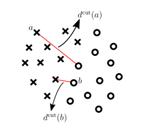
or both. We are in particular interested in binary partitions of the index set, i.e. and , corresponding to a binary principal submatrix partition . For such partitions we define the distance to the cut
| (81) |
Note that for the first term on the right hand side will be zero and the distance to the cut is thus defined as the distance to the closest vertex in , and vice versa for . This is illustrated in Figure 2. We will say that has the property of exponential decay away from the cut with constants and if
| (82) |
for all with and . We note that this is equivalent to the elements of satisfying the four conditions
| (83) |
for all . We shall in particular be concerned with sequences of matrices where each matrix is associated with a distance function , a binary partition of its index set, i.e. and , and the distance to the cut, defined as in (81),
| (84) |
Theorem 5.5.
Let be a sequence of matrices satisfying the assumptions of Theorem 5.1. Associate with each a binary partition of its index set and let be defined as in (84). Assume furthermore that for each distance , there are constants and independent of and a function such that
| (85) |
i.e. the number of vertices within distance from the cut is bounded by . Assume also that at least one of
| (86) |
hold for all . Then, for any each contains at most entries greater than in magnitude.
Proof 5.6.
For any matrix entry with magnitude greater than , (86) implies
| (87) |
By (85) the number of vertices within distance from the cut is bounded by , where is a constant independent of . Thus, only rows or columns may have entries with magnitude greater than and by Theorem 5.1, the number of entries in each row and column with magnitude greater than is bounded by a constant.
We will refer to the number of vertices within a given distance from the cut, i.e. , as the cut size. The function in (85) describes how the cut size increases with . Theorem 5.5 tells us that for a sequence of matrices with exponential decay with distance between vertices and exponential decay away from the cut, the number of significant entries does not grow faster than the cut size. Note that, in general, exponential decay away from the cut alone is not sufficient to reach this result. For example, assume that , so that the cut size grows as , and that both conditions in (86) are satisfied. Then, rows and columns may have entries with magnitude greater than , giving a total of matrix entries that may have magnitude greater than .
Theorem 5.7.
Let and be sequences of matrices with a common associated distance function for each . Assume that for any , there are constants and independent of such that
| (88) |
holds for all . For each , let be a subset of the index set and let , , and be positive and independent of .
-
(i)
Assume that
(89) (90) for all . Then, the entries of satisfy
(91) for any such that with independent of . This bound holds also with .
-
(ii)
Assume that
(92) (93) for all . Then, the entries of satisfy
(94) for any such that with independent of . This bound holds also with .
Proof 5.8.
We are particularly interested in the case of a binary partition of the index set and exponential decay away from the cut. The following result shows that multiplication of a matrix with exponential decay away from the cut with a matrix with exponential decay with distance between vertices gives a matrix with exponential decay away from the cut.
Corollary 5.9.
Let and be sequences of matrices with a common associated distance function for each . Assume that for any , there are constants and independent of such that
| (98) |
holds for all . For each , let , be a binary partition of the index set and assume that
| (99) | ||||
| (100) |
for all where and where , , and are positive and independent of . Then, the entries of satisfy
| (101) |
for any such that with independent of . This bound holds also with .
5.3 Localization in iterative refinement
In this section we will derive localization results for the matrices occurring in regular and localized iterative refinement. We will under certain assumptions show that while both Algorithms 1 and 2 involve only matrices that satisfy exponential decay with respect to distance between vertices, all matrices constructed in Algorithm 2 also satisfy exponential decay with respect to distance from the cut.
Theorem 5.11.
Let and be sequences of matrices with associated distance functions . Let each be Hermitian and partitioned as
| (102) |
and let
| (103) |
where and satisfy and , respectively. Let be the sequence of matrices produced by Algorithm 1 or Algorithm 2 with , , and a constant as input. For each iteration , until the stopping criterion is triggered, let
| (104) | ||||
| (105) | ||||
| (106) | ||||
| (107) | ||||
| (108) | ||||
| (109) | ||||
be the sequences of matrices corresponding to each of the intermediate matrices occurring in either one or both of Algorithm 1 and Algorithm 2. Assume that for any , there are constants and independent of such that
| (110) |
holds for all . Assume that and satisfy the exponential decay properties
| (111) | ||||
| (112) |
for all with constants and independent of . Assume also that the condition number of , , is uniformly bounded with respect to .
Then, each of the matrices in (104) through (109) satisfies an exponential decay property on the form
| (113) |
for any such that with independent of , where is any of the matrices in (104) through (109). Besides satisfying (113), the matrices in (105) through (109) also satisfy exponential decay away from the cut on the form
| (114) |
for any such that with independent of , where is any of the matrices in (105) through (109).
Lemma 5.12.
Let satisfy the exponential decay property with respect to distance between vertices
| (115) |
for all with positive constants and and assume that and . Then also satisfies the exponential decay property with respect to distance to cut
| (116) |
for all , where is defined as in (81).
Proof 5.13.
For all , we have that
| (117) |
and therefore
| (118) |
The same bounds clearly hold also for , and since all other entries are zero, the exponential decay property with respect to distance to cut is thus satisfied.
Proof 5.14 (Proof of Theorem 5.11).
Since is uniformly bounded, by (57) the number of iterations until the stopping criterion is triggered is also uniformly bounded. All matrices in (104) through (109) are therefore the result of a bounded number of matrix-matrix multiplications and additions. Repeated application of Theorem 5.3 implies the exponential decay property (113) for each matrix in (104) through (109).
By Lemma 5.12, the matrix satisfies an exponential decay property with respect to distance to the cut. Therefore and by Corollary 5.9 the matrix
| (119) |
also satisfies an exponential decay property with respect to distance to the cut. Corollary 5.9 also applies to the matrix since it is the result of multiplication of with (119). In fact, Corollary 5.9 may be applied to each matrix in (105) through (109) since a matrix with exponential decay away from the cut is involved in each product.
Theorem 5.1 and Theorem 5.11 imply that for any each matrix in (104) through (109) contains at most entries greater than in magnitude. Furthermore, the number of entries greater than in magnitude in each column or row is bounded by a constant independent of . Let be a function such that the cut size increases as with system size . Then, Theorem 5.5 and Theorem 5.11 imply that for any each matrix in (105) through (109) contains at most entries greater than in magnitude.
6 Recursive and localized inverse factorization
Associate with a binary principal submatrix tree corresponding to a recursive binary partition of the index set of . This recursive partitioning may continue down to single matrix elements or stop at some higher level.
Given such a binary principal submatrix tree, one can use Algorithm 1 in a recursive construction of an inverse factor. The matrix is split into four quadrants according to the binary partition of the index set, the method is called recursively on the two diagonal submatrices, and then the iterative refinement of Algorithm 1 is used to obtain the inverse factor of the whole matrix. Our recursive inverse factorization algorithm is given by Algorithm 3. Algorithm 3 was first proposed in [37], but includes here the new stopping criterion for iterative refinement presented in Section 3.3. On line 13 either one of the spectral and Frobenius matrix norms may be used.
Our localized inverse factorization, given by Algorithm 4, is obtained in essentially the same way, but makes use of the localized construction of starting guess and the localized iterative refinement of Algorithm 2.
Theorem 4.1 implies convergence of the iterative refinement for each level of the recursion in Algorithm 3 and 4. Furthermore, it follows from (54) and (55) that the bound of the number of iterations, needed to reach an accuracy , given by (57), holds for all levels in the recursion.
7 Numerical experiments
In this section the localization properties of the localized inverse factorization, i.e. Algorithm 4, are demonstrated. In all experiments, the recursion in Algorithm 4 is continued all the way down to single matrix elements where . In this way the final inverse factor is, up to differences due to floating point rounding, uniquely determined by Algorithm 4 and the recursive partition of the index set. In all numerical experiments was used in the iterative refinement and the Frobenius norm was used in the stopping criterion on line 14 of the algorithm.
Note that from a computational point of view it would likely be beneficial to stop the recursion at some predetermined larger block size and use for example the AINV algorithm [4] or one of its variants [2, 3, 40] to compute the inverse factor at the lowest level. The recursion may for example be stopped when there is no longer enough sparsity to take advantage of localization in and/or when the inverse factorization at that level will run serially, e.g. due to limited resources, so that the parallel features of the recursive algorithm will anyway not be utilized.
7.1 Simple lattices
Our first set of benchmark systems are chosen to clearly demonstrate the localization behavior for one-, two, and three-dimensional systems. The systems are also such that the results should be relatively easy to reproduce, not relying on auxiliary information, requiring extensive programming effort nor access to a supercomputer. We consider adjacency matrices corresponding to one-, two-, and three-dimensional integer lattices, i.e. a grid with unit spacing between nearest neighbors. Diagonal matrix entries are set to and matrix entries corresponding to edges between nearest neighbors on the lattice are set to . In the one-dimensional case this gives a tridiagonal matrix. In the two- and three-dimensional cases the vertices of the lattice are ordered using a recursive binary divide space procedure. At each level of the recursion the vertices are sorted along the greatest dimension and split in two subsets. Unless otherwise stated, we use the set of parameters in Table 1.
| Lattice | No. of vertices | ||
|---|---|---|---|
| 512 | 1 | 0.25 | |
| 1 | 0.05 | ||
| 1 | 0.01 |
7.1.1 Localization in inverse factor
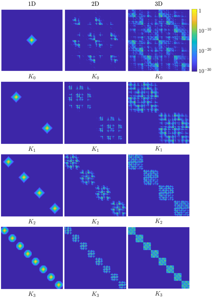
Figure 3 demonstrates the localization in the final inverse factor produced by Algorithm 4 for the 1D, 2D, and 3D lattice systems. Note that, in the upper panels showing images of the -matrices, a single blue color is used to indicate matrix elements with absolute value smaller than . Although not visible in the figures, the decay of course continues below .
In the image of in the upper left panel for the one-dimensional system the matrix element magnitude clearly decays away from the diagonal which in this case corresponds to decay with distance between vertices. This decay with distance is more difficult to grasp looking only at the images in the upper panels for the two- and three-dimensional systems. However, the lower panels reveals an even faster decay with distance for the two- and three-dimensional systems, which is due to the smaller matrix entries corresponding to edges between nearest neighbors determined by the parameter , see Table 1.

7.1.2 Localization in correction matrices
The complete recursion in Algorithm 4 can be seen as a sequence of corrections to the inverse factor, i.e. where the subscript denotes the level of recursion with being the correction at the root level of the recursion and is the number of recursion levels. The correction matrix is a block diagonal matrix, where each block corresponds to a node of the binary tree of recursive calls at level and is, for , equal to the sum of the matrices in the iterative refinement corresponding to this node. The matrix is, in our case where we continue the recursion down to single matrix elements, the diagonal matrix given by . Note that for , the correction matrix spans all branches in the binary tree of recursion at level . We will use the correction matrices as representatives for the matrices in Algorithm 4 corresponding to the matrices in (105) through (109), which all show similar localization behavior.
Figure 4 shows images of the correction matrices for , for the one-, two-, and three-dimensional lattice benchmark systems. It may be noted that these figures correspond directly to the images of in Figure 3. One may for example note that the upper right and lower left quadrants of are identical to the corresponding submatrices of . This is expected as correction to those submatrices only occurs at the root level of the recursion. Again the localization, with rapid decay away from the cut (or cuts for ), is clearly seen in the one-dimensional case, but not as easily seen in the two- and three-dimensional cases.
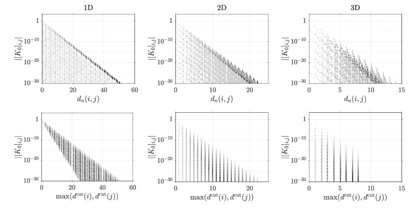
To more clearly see the localization behavior we plot in Figure 5 the decay with distance between vertices and the decay away from the cut for the root level correction matrices . Clearly, there is rapid decay both with distance between vertices and away from the cut, which may be compared to the decay in the matrices seen in the lower panels in Figure 3.
The key advantage of the localized inverse factorization of Algorithm 4 over the regular recursive inverse factorization of Algorithm 3 is its superior localization properties. Algorithm 3 includes products of matrices that feature localization of the type seen in Figure 3, i.e. exponential decay with distance between vertices. See for example the construction of on line 12 of Algorithm 3 with matrix products involving and . Algorithm 4, on the other hand, involves only operations, matrix products and additions, where at least one of the matrices feature localization of the type seen in Figures 4 and 5. This means that, if only matrix elements of significant magnitude are included in the calculation, the computational cost of Algorithm 4 may be way lower than that of Algorithm 3.
7.1.3 Localization with increasing system size
So far all calculations have been for the fixed system sizes given in Table 1. We are now interested in how the localization changes with increasing system size. We consider again adjacency matrices corresponding to integer lattices but with increasing dimension. We set the parameters and as in Table 1. We consider one-dimensional grids with 8, 16, 32, 64, 128, 256, and 512 vertices, two-dimensional grids with vertices where , and three-dimensional grids with vertices where .
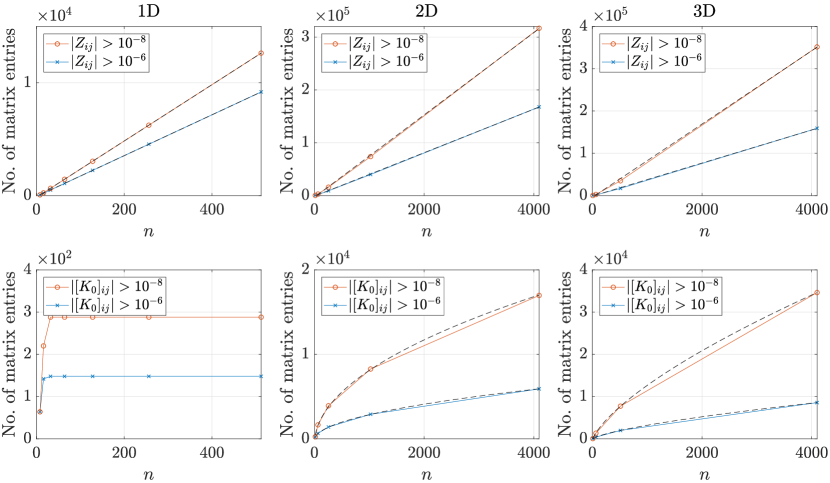
To see how the localization changes with system size we plot in Figure 6 the number of matrix entries in and whose absolute value is above a given threshold value with increasing system size. For the final inverse factor the number of significant matrix entries increases linearly with system size which is consistent with an exponential decay with respect to distance between vertices with and independent of , see Theorem 5.1.
For the correction matrices Figure 6 displays very different behavior for the one-, two-, and three-dimensional systems. This can be understood by considering how the cut size varies with system size. In the 1D case, the number of vertices within any fixed distance from the cut, i.e. the cut size, is bounded by a constant independent of . In the 2D case, the cut size increases as and in the 3D case, the cut size increases as . We recall from Theorem 5.5 that a matrix that satisfies both exponential decay with distance between vertices and away from a cut with cut size contains at most entries with magnitude greater than any given constant . The nearly perfect least squares fits in the lower panels of Figure 6 indicate that the number of entries in increases as , , and for the 1D, 2D, and 3D cases respectively. The results in the lower panels of Figure 6 are therefore consistent with satisfying both exponential decay with respect to distance between vertices and away from the cut with and independent of .
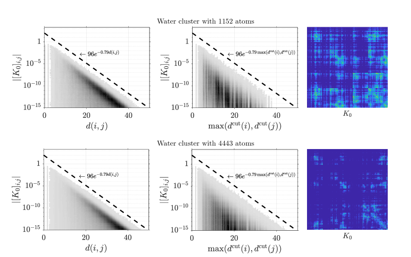
7.2 Alkane chains and water clusters
We consider here application of the localized inverse factorization to basis set overlap matrices occurring in Hartree–Fock and Kohn–Sham density functional theory electronic structure calculations using standard Gaussian basis sets. The overlap matrices were generated using the Ergo open-source program for linear-scaling electronic structure calculations [45], publicly available at ergoscf.org under the GNU Public License (GPL) v3. In the case of such overlap matrices, each vertex corresponds to a basis function center and we let the distance function be the Euclidean distance between basis function centers and . The magnitude of matrix entries decays as which is even faster than exponential decay [38]. In all calculations the standard Gaussian basis set STO-3G was used. Similarly to the calculations on the lattice systems the basis functions were ordered using a recursive binary divide space procedure based on the coordinates of the basis function centers.
We consider overlap matrices for alkane chains and water clusters. We
run calculations with two different sizes for each type of system to
be able to see if the exponential decay properties are retained when
the system size is increased. The alkane chain xyz coordinates were
generated using the generate_alkane.cc program included in
the Ergo source code package. The water cluster xyz coordinates,
originally used in [44], are available for
download at ergoscf.org.
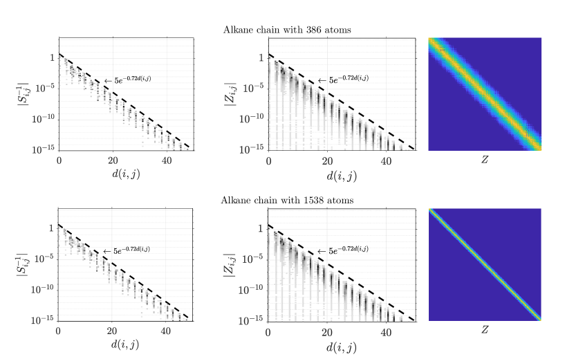
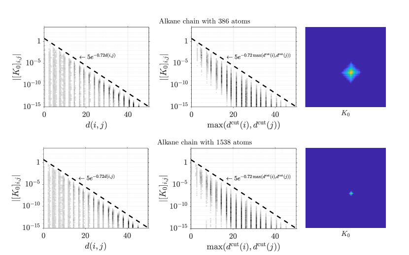
Localization results for the alkane chains are plotted in Figures 7 and 8. Figure 7 shows the magnitude of the matrix entries in and as functions of distance between vertices or basis function centers along with an image of indicating the magnitude of the matrix entries as in previous figures. Figure 8 shows the magnitude of the matrix entries in as a function of distance between vertices and as a function of distance away from the cut along with an image of . The matrix dimensions in the 386 atom and 1538 atom cases are 898 and 3586, respectively. These numbers, in contrast to the 1D lattice system considered above, are not powers of 2, which explains why significant matrix entries of in Figure 8 corresponding to atom centers close to the cut are not located at the center of the matrix. The corresponding localization results for the water clusters are plotted in Figures 9 and 10. The dashed help lines makes it easy to see that the exponential decay properties are retained for all matrices , , and and for both types of systems.

8 Concluding remarks
Previous work on the computation of inverse factors has to large extent focused on approximations used as preconditioners for iterative solution of linear systems [5]. Examples, besides the AINV algorithms already mentioned, include FSAI [23] and more recent variants [11]. Methods making use of a recursive partitioning of the matrix is used in direct methods for factorization such as multifrontal methods [10]. In this case the matrix is seen as the adjacency matrix of a graph and the matrix is partitioned using a three-by-three block partition corresponding to a vertex separator of the graph. Multifrontal methods have typically been used for example for the Cholesky decomposition and not its inverse factor. However, the multifrontal approach could also be combined with the AINV algorithm for direct computation of the inverse Cholesky factor. A starting guess for iterative refinement is in [31] built up from the inverse factors of overlapping principal submatrices. The convergence has not been proven but this approach could possibly lead to a lower initial factorization error and reduced number of iterative refinement iterations compared to our binary partition at the expense of more computations to construct the starting guess. Note though that for large enough systems with localization we have, under certain assumptions, shown that the cost of our localized inverse factorization is completely dominated by the solutions of the subproblems and not the iterative refinement used to glue together their solutions.
A strength of the localized inverse factorization algorithms is the proved convergence for any binary partition of the index set. Inappropriate partitions at worst lead to poor localization and higher computational cost. We used in our numerical experiments a straightforward space-dividing algorithm for the recursive binary partition of the index set. More advanced partitioning algorithms could take into account the magnitude of the entries in and attempt to minimize the cut size and the initial factorization error.
Our localized inverse factorization algorithm could be combined with some direct inverse factorization method that is efficient for small dense or semi-sparse systems. In the numerical experiments we continued the recursion all the way down to single matrix elements. It would in general be more efficient to stop the recursion as soon as the matrix size is smaller than some predetermined block size and use for example one of the AINV algorithms to compute the inverse factor. Another possibility is to use regular recursive inverse factorization for intermediate levels in the recursion.
We showed in Section 5 that under certain assumptions both the regular and localized iterative refinement of Algorithms 1 and 2 involve only matrices with exponential decay with distance between vertices. However, all matrices involved in Algorithm 2 also have the property of exponential decay away from the cut. This means that whereas the number of significant matrix entries in Algorithm 1 grows not faster than , the number of significant matrix entries in Algorithm 2 also does not grow faster than the cut size. For binary partitions with a cut size increasing as and large enough systems the localized algorithm is therefore superior to the regular version. Note that we have not provided a rigorous proof for the localization features of the full recursive and localized inverse factorization algorithms demonstrated in Section 7. There are two important differences compared to Algorithms 1 and 2. Firstly, it is difficult to come up with a strict bound for the number of iterations since the stopping criterion relies on stagnation due to numerical errors. Secondly, the computed inverse factor is the result of a sum over correction matrices, where is the number of levels in the recursion. Clearly, tends to infinity together with so that the number of correction matrices in the sum tends to infinity with increasing , which entails another difficulty. Nevertheless, all our numerical experiments indicate that the localization properties of Algorithms 1 and 2 are inherited by their recursive counterparts. Furthermore, our results indicate that the total computational cost can increase linearly with system size if negligible matrix entries are not stored nor included in the calculation. In summary, the theoretical results of Section 5 together with the numerical experiments of Section 7 make us confident that the localized inverse factorization, especially with regard to localization, represents a dramatic improvement over the regular recursive inverse factorization.
The localized inverse factorization is also well suited for parallelization. The two subproblems of computing inverse factors of the two principal submatrices at each level of the recursion are completely disconnected and can thus be solved in parallel without any communication in between. For systems with localization, any communication needed in the iterative refinement step to combine the subproblem solutions involves only data close to the cut. Using an appropriate partition of the index set, the cut size is vanishingly small in proportion to the total problem size for large enough systems.
This work did not concern computational details regarding how to select matrix entries for removal or other implementation issues such as how to best parallelize the method on a particular computer architecture. The efficient implementation of the localized inverse factorization algorithm will be considered elsewhere.
References
- [1] M. Benzi, P. Boito, and N. Razouk, Decay properties of spectral projectors with applications to electronic structure, SIAM Rev., 55 (2013), pp. 3–64.
- [2] M. Benzi, J. K. Cullum, and M. Tuma, Robust approximate inverse preconditioning for the conjugate gradient method, SIAM J. Sci. Comput., 22 (2000), pp. 1318–1332.
- [3] M. Benzi, R. Kouhia, and M. Tuma, Stabilized and block approximate inverse preconditioners for problems in solid and structural mechanics, Comput. Meth. Appl. Mech. Eng., 190 (2001), pp. 6533–6554.
- [4] M. Benzi, C. D. Meyer, and M. Tuma, A sparse approximate inverse preconditioner for the conjugate gradient method, SIAM J. Sci. Comput., 17 (1996), pp. 1135–1149.
- [5] M. Benzi and M. Tuma, A comparative study of sparse approximate inverse preconditioners, Appl. Numer. Math., 30 (1999), pp. 305 – 340.
- [6] D. A. Bini, N. J. Higham, and B. Meini, Algorithms for the matrix pth root, Numer. Algorithms, 39 (2005), pp. 349–378.
- [7] M. Challacombe, A simplified density matrix minimization for linear scaling self-consistent field theory, J. Chem. Phys., 110 (1999), pp. 2332–2342.
- [8] S. H. Cheng, N. J. Higham, C. S. Kenney, and A. J. Laub, Approximating the logarithm of a matrix to specified accuracy, SIAM J. Matrix Anal. A., 22 (2001), pp. 1112–1125.
- [9] J. D. Cloizeaux, Energy bands and projection operators in a crystal: Analytic and asymptotic properties, Phys. Rev., 135 (1964), pp. A685–A697.
- [10] T. A. Davis, S. Rajamanickam, and W. M. Sid-Lakhdar, A survey of direct methods for sparse linear systems, Acta Numer., 25 (2016), pp. 383–566.
- [11] A. Franceschini, V. Paludetto Magri, M. Ferronato, and C. Janna, A robust multilevel approximate inverse preconditioner for symmetric positive definite matrices, SIAM J. Matrix Anal. A., 39 (2018), pp. 123–147.
- [12] N. J. Higham, Stable iterations for the matrix square root, Numer. Algorithms, 15 (1997), pp. 227–242.
- [13] N. J. Higham, Functions of matrices : theory and computation, SIAM, Philadelphia, 2008.
- [14] N. J. Higham, D. S. Mackey, N. Mackey, and F. Tisseur, Functions preserving matrix groups and iterations for the matrix square root, SIAM J. Matrix Anal. A., 26 (2005), pp. 849–877.
- [15] A. Holas, Transforms for idempotency purification of density matrices in linear-scaling electronic-structure calculations, Chem. Phys. Lett., 340 (2001), pp. 552–558.
- [16] R. A. Horn and C. R. Johnson, Matrix Analysis, Cambridge University Press, New York, NY, USA, 2nd ed., 2012.
- [17] B. Jansík, S. Høst, P. Jørgensen, J. Olsen, and T. Helgaker, Linear-scaling symmetric square-root decomposition of the overlap matrix, J. Chem. Phys., 126 (2007), p. 124104.
- [18] C. Kenney and A. Laub, Rational iterative methods for the matrix sign function, SIAM J. Matrix Anal. A., 12 (1991), pp. 273–291.
- [19] C. Kenney and A. Laub, On scaling Newton’s method for polar decomposition and the matrix sign function, SIAM J. Matrix Anal. A., 13 (1992), pp. 688–706.
- [20] J. Kim and Y. Jung, A perspective on the density matrix purification for linear scaling electronic structure calculations, Int. J. Quantum Chem., 116 (2016), pp. 563–568.
- [21] W. Kohn, Analytic properties of Bloch waves and Wannier functions, Phys. Rev., 115 (1959), pp. 809–821.
- [22] W. Kohn, Density functional and density matrix method scaling linearly with the number of atoms, Phys. Rev. Lett., 76 (1996), pp. 3168–3171.
- [23] L. Kolotilina and A. Yeremin, Factorized sparse approximate inverse preconditionings I. Theory, SIAM J. Matrix Anal. A., 14 (1993), pp. 45–58.
- [24] A. Kruchinina, E. Rudberg, and E. H. Rubensson, Parameterless stopping criteria for recursive density matrix expansions, J. Chem. Theory Comput., 12 (2016), pp. 5788–5802.
- [25] X.-P. Li, R. W. Nunes, and D. Vanderbilt, Density-matrix electronic-structure method with linear system-size scaling, Phys. Rev. B, 47 (1993), pp. 10891–10894.
- [26] P.-O. Löwdin, Quantum theory of cohesive properties of solids, Adv. Phys., 5 (1956), p. 1.
- [27] A. Marek, V. Blum, R. Johanni, V. Havu, B. Lang, T. Auckenthaler, A. Heinecke, H.-J. Bungartz, and H. Lederer, The ELPA library: scalable parallel eigenvalue solutions for electronic structure theory and computational science, J. Phys.: Condens. Matter, 26 (2014), p. 213201.
- [28] R. S. Martin and J. H. Wilkinson, Reduction of the symmetric eigenproblem Ax=Bx and related problems to standard form, Numer. Math., 11 (1968), pp. 99–110.
- [29] P. E. Maslen, C. Ochsenfeld, C. A. White, M. S. Lee, and M. Head-Gordon, Locality and sparsity of ab initio one-particle density matrices and localized orbitals, J. Phys. Chem. A, 102 (1998), pp. 2215–2222.
- [30] R. McWeeny, The density matrix in self-consistent field theory. I. Iterative construction of the density matrix, Proc. R. Soc. London Ser. A, 235 (1956), pp. 496–509.
- [31] C. F. A. Negre, S. M. Mniszewski, M. J. Cawkwell, N. Bock, M. E. Wall, and A. M. N. Niklasson, Recursive factorization of the inverse overlap matrix in linear-scaling quantum molecular dynamics simulations, J. Chem. Theory Comput., 12 (2016), pp. 3063–3073.
- [32] A. M. N. Niklasson, Expansion algorithm for the density matrix, Phys. Rev. B, 66 (2002), p. 155115.
- [33] A. M. N. Niklasson, Iterative refinement method for the approximate factorization of a matrix inverse, Phys. Rev. B, 70 (2004), p. 193102.
- [34] B. Philippe, An algorithm to improve nearly orthonormal sets of vectors on a vector processor, SIAM J. Algebra. Discr., 8 (1987), pp. 396–403.
- [35] D. Richters, M. Lass, C. Plessl, and T. D. Kühne, A general algorithm to calculate the inverse principal -th root of symmetric positive definite matrices, 2017, https://arxiv.org/abs/arXiv:1703.02456.
- [36] E. H. Rubensson, Nonmonotonic recursive polynomial expansions for linear scaling calculation of the density matrix, J. Chem. Theory Comput., 7 (2011), pp. 1233–1236.
- [37] E. H. Rubensson, N. Bock, E. Holmström, and A. M. N. Niklasson, Recursive inverse factorization, J. Chem. Phys., 128 (2008), p. 104105.
- [38] E. H. Rubensson and E. Rudberg, Bringing about matrix sparsity in linear-scaling electronic structure calculations, J. Comput. Chem., 32, pp. 1411–1423.
- [39] E. H. Rubensson and E. Rudberg, Locality-aware parallel block-sparse matrix-matrix multiplication using the Chunks and Tasks programming model, Parallel Comput., 57 (2016), pp. 87–106.
- [40] E. H. Rubensson, E. Rudberg, and P. Sałek, A hierarchic sparse matrix data structure for large-scale Hartree-Fock/Kohn-Sham calculations, J. Comput. Chem., 28 (2007), pp. 2531–2537.
- [41] E. H. Rubensson, E. Rudberg, and P. Sałek, Density matrix purification with rigorous error control, J. Chem. Phys., 128 (2008), p. 074106.
- [42] E. H. Rubensson, E. Rudberg, and P. Salek, Methods for Hartree-Fock and Density Functional Theory Electronic Structure Calculations with Linearly Scaling Processor Time and Memory Usage, Springer Netherlands, Dordrecht, 2011, pp. 263–300.
- [43] E. Rudberg and E. H. Rubensson, Assessment of density matrix methods for linear scaling electronic structure calculations, J. Phys.: Condens. Matter, 23 (2011), p. 075502.
- [44] E. Rudberg, E. H. Rubensson, and P. Sałek, Kohn–Sham density functional theory electronic structure calculations with linearly scaling computational time and memory usage, J. Chem. Theory Comput., 7 (2011), pp. 340–350.
- [45] E. Rudberg, E. H. Rubensson, P. Sałek, and A. Kruchinina, Ergo: An open-source program for linear-scaling electronic structure calculations, SoftwareX, 7 (2018), pp. 107–111.
- [46] W. Rudin, Principles of Mathematical Analysis, McGraw-Hill, Singapore, 1976.
- [47] G. W. Stewart and J. Sun, Matrix perturbation theory, Academic Press, San Diego, 1990.
- [48] P. Suryanarayana, Optimized purification for density matrix calculation, Chem. Phys. Lett., 555 (2013), pp. 291 – 295.
- [49] J. VandeVondele, U. Borštnik, and J. Hutter, Linear scaling self-consistent field calculations with millions of atoms in the condensed phase, J. Chem. Theory Comput., 8 (2012), pp. 3565–3573.
- [50] A. Von Ostrowski, Über eigenwerte von produkten hermitescher matrizen, Abh. Math. Semin. Univ. Hambg., 23 (1959), pp. 60–68.