Multi-messenger Bayesian parameter inference of a binary neutron-star merger

Abstract

The combined detection of a binary neutron-star merger in both gravitational waves (GWs) and electromagnetic (EM) radiation spanning the entire spectrum – GW170817 / AT2017gfo / GRB170817A – marks a breakthrough in the field of multi-messenger astronomy. Between the plethora of modeling and observations, the rich synergy that exists among the available data sets creates a unique opportunity to constrain the binary parameters, the equation of state of supranuclear density matter, and the physical processes at work during the kilonova and gamma-ray burst. We report, for the first time, Bayesian parameter estimation combining information from GW170817, AT2017gfo, GRB170817 to obtain truly multi-messenger constraints on the tidal deformability $\tilde{\Lambda}\in[302,860]$, total binary mass $M\in[2.722,2.751]M_{\odot}$, the radius of a $1.4$ solar mass neutron star $R\in[11.3,13.5]\rm km$ (with additional $0.2\ \rm km$ systematic uncertainty), and an upper bound on the mass ratio of $q\leq 1.27$, all at 90% confidence. Our joint novel analysis makes use of new phenomenological descriptions of the dynamical ejecta, debris disk mass, and remnant black hole properties, all derived from a large suite of numerical relativity simulations.

1 Introduction

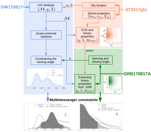
Figure 1: Flow chart of the analysis showcasing how the analysis of GW170817, AT2017gfo, and GRB170817A. At the bottom of the panel, we show KDE posterior distributions of the tidal deformability (left panel) and the mass ratio (right panel). The final multi-messenger result is shown as a shaded region, where the 90% confidence interval is shaded darker. For the mass ratio, we assume a $90\%$ upper limit and for the tidal deformability we mark the $5$ and $95$ percentiles.

The combined detection of a GW event, GW170817 (Abbott et al., 2017a), a gamma ray burst (GRB) of short duration, GRB170817A (Abbott et al., 2017c) accompanied by a non-thermal afterglow, and thermal emission (“kilonova”) at optical, near-infrared, and ultraviolet wavelengths, AT2017gfo (Abbott et al., 2017b; Arcavi et al., 2017; Coulter et al., 2017; Lipunov et al., 2017; Soares-Santos et al., 2017; Tanvir et al., 2017; Valenti et al., 2017) from a binary neutron star (BNS) merger has enabled major leaps forward in several research areas. The latter include new limits on the equation of state (EOS) of cold matter at supranuclear densities (e.g. De et al. (2018); Abbott et al. (2018); Radice et al. (2018b); Radice & Dai (2019); Coughlin et al. (2018); Bauswein et al. (2017); Annala et al. (2018); Most et al. (2018); Ruiz et al. (2018); Margalit & Metzger (2017); Rezzolla et al. (2018); Shibata et al. (2017)). One of the main goals of the nascent field of “multi-messenger astronomy" is to obtain complementary observations of the same object or event. These observations, potentially across a variety of wavelengths and particle types, probe different aspects of the system. In the case of GW170817, GW detectors such as LIGO and Virgo provide a highly accurate measurement of the binary chirp mass $\mathcal{M}=1.186M_{\odot}$, but leave the mass ratio, $q$, poorly constrained.

A variety of studies over the last year focused on the properties of this first detection of a BNS system, including detailed analyses of the GW signal by the LVC (e.g. Abbott et al. (2017a, 2019a, 2018, 2019b)) and external groups (e.g. De et al. (2018); Finstad et al. (2018); Dai et al. (2018)), relying on different parameter estimation techniques and a variety of GW models. Despite this diversity of methods, all of the published works predict small tidal deformabilities, favoring relatively soft EOSs and placing upper limits on the radii of NSs. For this first BNS system the GW analyses broadly agree, and studies indicate that systematic errors are below the statistical errors (Abbott et al., 2019a; Dudi et al., 2018; Samajdar & Dietrich, 2018). However, this might not be the case for future GW observations with larger signal-to-noise ratios, thus emphasizing the need for further improvements in the current infrastructure and GW modeling.

Fortunately, deficiencies in the available GW information can sometimes be supplemented with EM observations, potentially improving the measurements of key parameters. For instance, the results of numerical relativity simulations were used to argue against the EOS being too soft, as the mass of the remnant accretion disk and its associated wind ejecta would be insufficient to account for the luminosity of the observed kilonova, e.g., Radice et al. (2018a); Bauswein et al. (2017); Coughlin et al. (2018). Combining GW and EM observations thus provides an opportunity to independently constrain the binary parameters, place tighter bounds on the EOS, and obtain a better understanding of the physical processes and outcomes of BNS mergers.

One of the first multi-messenger constraints on the tidal deformability and supranuclear EOS was presented in Radice et al. (2018b). Based on numerical relativity (NR) simulations, the authors proposed that the tidal deformability needs to be $\tilde{\Lambda}\geq 400$ to ensure that a significant fraction of matter was either ejected from the system or contained within a debris disk around the BH remnant to explain the bright EM counterpart. Recently, Radice & Dai (2019) updated this first analysis and obtained constraints on the tidal deformability of $\tilde{\Lambda}\in(323,776)$ and on the corresponding radius of a 1.4 $M_{\odot}$ neutron star of $12.2^{+1.0}_{-0.8}\pm 0.2$ km, performing a multi-messenger parameter estimation incorporating information from the disk mass (Radice et al., 2018c). To the best of our knowledge, Coughlin et al. (2018) presented the first analysis of the lightcurves and spectra of AT2017gfo linking with a Bayesian analysis the kilonova properties to the source properties of the binary. We used the kilonova model of Kasen et al. (2017) combined with methods of Gaussian Process Regression (GPR, Doctor et al. (2017); Pürrer (2014); Coughlin et al. (2018)), and related a fraction of the ejected material to dynamical ejecta. Based on the analysis, the tidal deformability was limited to $\tilde{\Lambda}>197$.

In addition, there have been studies placing limits on the maximum NS mass of a stable TOV star, $M_{\rm TOV}$. Those studies are orthogonal to the works constraining the tidal deformability since both quantities $(\tilde{\Lambda},M_{\rm TOV})$ test different parts of the NS EOS. Margalit & Metzger (2017) places a $90\%$ upper limit on the mass of a non-rotating NS of $2.17M_{\odot}$, Rezzolla et al. (2018) report a maximum TOV mass of $2.16^{0.17}_{0.15}M_{\odot}$, and Shibata et al. (2017) provide an estimate for the maximum mass of $2.15-2.25M_{\odot}$. All these constraints have been derived by assuming the formation of a BH after the merger of GW170817 and incorporating the measured chirp mass inferred from the GW analysis. We employ for our analysis the maximum mass constraint derived in Margalit & Metzger (2017). There has also been an effort to investigate the nature of GW170817, with regards to the possibility of a BNS or NSBH source, e.g. Hinderer et al. 2019; Coughlin & Dietrich 2019. For example, Hinderer et al. 2019 used numerical-relativity simulations and a joint analysis of GW and EM measurements to show that $<$40% of the binary parameters consistent with the GW data are compatible with EM observations.

While overall many analyses of GW170817 and its electromagnetic signatures have been presented in the literature, we will present here the first to combine information from all three channels: GW170817, GRB170817A, and AT2017gfo. Our work makes use of more available knowledge than employed in any previous multi-messenger analyses. In particular, our final posteriors describe the observed GW signature, the lightcurve data of AT2017gfo, and explain the properties of GRB170817A. The flowchart in Fig. 1 highlights the interplay between the different observable signatures and presents the joint posteriors obtained on the tidal deformability $\tilde{\Lambda}$, the binary mass ratio $q$, and the maximum mass of a stable non-rotating neutron star $M_{\rm TOV}$.

2 Analysis

2.1 GW170817

We begin by analyzing GW170817 (blue shaded region of Fig. 1) and use the publicly available “low spin” posterior samples (https://dcc.ligo.org/LIGO-P1800370, Abbott et al. (2019b)). As these sample use the sky localization obtained from EM observations, they already incorporate EM information. Under the assumption that the merging objects are two NSs described by the same EOS (De et al., 2018; Abbott et al., 2018), we can further restrict the posterior distribution. For this purpose, we use the posterior samples of Carson et al. (2019) where a same spectral EOS representation for both stars is employed. Finally, we discard those systems with viewing angles which are inconsistent with the ones obtained from the GRB afterglow by Troja et al. (2019).

2.2 AT2017gfo

In the second phase of our work, we analyze the light curves of AT2017gfo (red shaded region in Fig. 1). We fit the observational data (Coughlin et al., 2018; Smartt et al., 2017; Abbott et al., 2017b) with the 2-component radiative transfer model of Kasen et al. (2017). The usage of multiple components, proposed prior to the discovery of GW170817 (Metzger & Fernández, 2014), is motivated by different ejecta mechanisms contributing to the total $r$-process yields of BNS mergers. The first type of mass ejection are “dynamical ejecta" generated during the merger process itself. Dynamical ejecta are typically characterized by a low-electron fraction when they are created by tidal torque, but the electron fraction can extend to higher values (and thus the lanthanide abundance be reduced) in the case of shock-driven ejecta. In addition to dynamical ejecta, disk winds driven by neutrino energy, magnetic fields, viscous evolution and/or nuclear recombination (e.g. Kohri et al. (2005); Surman et al. (2006); Metzger et al. (2008); Dessart et al. (2009); Fernández & Metzger (2013); Perego et al. (2014); Siegel et al. (2014); Just et al. (2015); Rezzolla & Kumar (2015); Ciolfi & Siegel (2015); Siegel & Metzger (2017)) leads to a large quantity of ejecta, which in many cases exceeds that of the dynamical component. The ejecta components employed in our kilonova light curve analysis are related to these different physical ejecta mechanisms: the first ejecta component is assumed to be proportional to dynamical ejecta, $m_{\rm ej,1}=\alpha^{-1}\ m_{\rm dyn}$, while the second ejecta component arises from the disk wind and is assumed to be proportional to the mass of the remnant disk, $m_{\rm ej,2}=\zeta\ m_{\rm disk}$. By fitting the observed lightcurves with the kilonova models (Kasen et al., 2017) withing a GPR framework (Coughlin et al., 2018), we obtain for each component posterior distributions for the ejecta mass $m_{\rm ej}$, the lanthanide mass fraction $X_{\rm lan}$ (related to the initial electron fraction), and the ejecta velocity $v_{\rm ej}$.

The values of $m_{\rm ej}$, $X_{\rm lan}$, and $v_{\rm ej}$ obtained from our kilonova analysis are related to the properties of the binary and EOS using new phenomenological fits to numerical relativity simulations, which we briefly described below. First, we revisit the phenomenological fit presented in Radice et al. (2018c) between the disk mass and tidal deformability $\tilde{\Lambda}$ to correlate the disk mass, $m_{\rm disk}$, to the properties of the merging binary. Simulations following the merger aftermath suggest that the disk mass is accumulated primarily through radial redistribution of matter in the post-merger remnant. Thus, the lifetime of the remnant prior to its collapse is related to its stability and found to strongly correlate with the disk mass (Radice et al., 2018a). We find that the lifetime in turn is governed to a large degree by the ratio of $M/M_{\rm thr}$, where $M$ is the total binary mass and $M_{\rm thr}$ is the threshold mass (Bauswein et al., 2013) above which the merger results in prompt (dynamical timescale) collapse to a black hole, which depends on the NS compactness and thus $\tilde{\Lambda}$. Therefore, $M/M_{\rm thr}$, rather than $\tilde{\Lambda}$ alone, provides a better measure of the stability of the post-merger remnant, and following the arguments above, is expected to correlate with $m_{\rm disk}$.

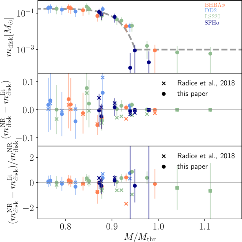
Figure 2: Disk masses as a function of the ratio between the total mass and the threshold mass for prompt BH formation. The disk mass estimates are obtained from the numerical relativity simulations presented in Radice et al. (2018c). The errorbars refer to $(0.5m_{\rm disk}+5\times 10^{-4}M_{\odot})$ as stated in the original work of (Radice et al., 2018c). The threshold mass for prompt BH formation is computed following Bauswein et al. (2013). We present our best fit, Eq. (14), in the top panel and show the absolute and fractional errors of the phenomenological fit in the middle and bottom panel. We compare our results with the original version of the fit presented in Radice et al. (2018c).

Fig. 2 shows, based on the suite of numerical relativity simulations of Radice et al. (2018c), that there indeed exists a relatively tight correlation between the accretion disk mass and $M/M_{\rm thr}$. For our analysis, we will use

$$\log_{10} \left(m_{\rm disk}\left[M_{\rm tot}/M_{\rm thr}\right]\right)=$$

$$\max\left(-3,\ a\left(1+b\tanh\left[\frac{c-M_{\rm tot}/M_{\rm thr}}{d}\right]\right)\right),$$ (1)

with $M_{\rm thr}(M_{\rm TOV},R_{1.6{M_{\odot}}})$ as discussed in Bauswein et al. (2013) and the Appendix, to describe the disk mass. The fitting parameters of Eq. (14) are $a=-31.335$, $b=-0.9760$, $c=1.0474$, $d=0.05957$.

Connecting the NS radius to the chirp mass and tidal deformability, $R=\mathcal{M}(\tilde{\Lambda}/a)^{1/6}$ (De et al., 2018), we conclude that the disk mass (and thus the disk wind ejecta) is a function of the tidal deformability, total binary mass, and the maximum TOV mass, $M_{\rm TOV}$. Therefore, both information, those on the densest portion of the EOS, which controls $M_{\rm TOV}$, and those from lower densities, as encoded in $\tilde{\Lambda}$ or $R_{1.6M\odot}$, play a role in controlling the disk mass and kilonova properties. The inclusion of these parameters and slight changes in the functional form of the phenomenological relation decrease the average fractional errors by more than a factor of 3 relative to previous disk mass estimates based on $\tilde{\Lambda}$ alone (Radice et al., 2018a), thus reducing uncertainties and errors on the EOS constraints obtained from kilonova observations.

Another key ingredient in our analysis is the role of the dynamical ejecta as the first kilonova ejecta component. Based on a suite of numerical relativity simulations obtained by different groups and codes, Dietrich & Ujevic (2017) derived the first phenomenological fit for the dynamical ejecta for BNS systems. This fit (in its original or upgraded version) has been employed in a number of studies, including the analysis of GW170817 (Abbott et al., 2017d; Coughlin et al., 2018), and they have been updated in Coughlin et al. (2018) and Radice et al. (2018c). Here, we present a further upgrade which incorporates the new numerical relativity dataset of Radice et al. (2018c) and uses the fitting function of Coughlin et al. (2018) (which fits $\log_{10}m_{\rm dyn}$ instead of $m_{\rm dyn}$). The extended dataset contains a total of 259 numerical relativity simulations. The final fitting function is

$$\log_{10}m_{\rm dyn}^{\rm fit}=\left[a\frac{(1-2\ C_{1})M_{1}}{C_{1}}+b\ M_{2}\left(\frac{M_{1}}{M_{2}}\right)^{n}+\frac{d}{2}\right]+[1\leftrightarrow 2],$$ (2)

with $a=-0.0719$, $b=0.2116$, $d=-2.42$, and $n=-2.905$ and $C_{1,2}$ denoting the compactnesses of the individual stars, a more detailed discussed can be found in the Appendix.

A final ingredient in relating observational data to the binary parameters are phenomenological fits for the BH mass and spin. One finds that with an increasing total mass $M$, the final black hole mass and angular momentum increases almost linearly. For unequal mass mergers, $M_{\rm BH}$ and $\chi_{\rm BH}$ decrease with $M$. Considering the imprint of the EOS, we find that for larger values of $\tilde{\Lambda}$, the final black hole mass decreases, which follows from the observation that the disk mass increases with $\tilde{\Lambda}$. We finally obtain:

$$M_{\rm BH}=a\left(\frac{\nu}{0.25}\right)^{2}\left(M+b\ \frac{\tilde{\Lambda}}{400}\right)$$ (3)

with $a=0.980$ and $b=-0.093$ and

$$\chi_{\rm BH}=\tanh\left[a\nu^{2}(M+b\ \tilde{\Lambda})+c\right]$$ (4)

with $a=0.537$, $b=-0.185$, and $c=-0.514$; further details are given in the Appendix.

In addition to using these fits, we use the results of Margalit & Metzger (2017), who derive a $90\%$ upper limit on the mass of a non-rotating NS of $2.17M_{\odot}$ based on energetic considerations from the GRB and kilonova which rule out a long-lived supramassive NS remnant, to place a prior on $M_{\rm TOV}$ between 2–2.17 $M_{\odot}$. Combining these phenomenological relations with the lightcurve data, our analysis strongly favors equal or nearly equal mass systems and $\tilde{\Lambda}\geq 400$ (see appendix). We conclude that roughly $20\%$ of the first ejecta component is associated with dynamical ejecta, while about $20\%$ of the disk mass must be ejected in winds to account for the second ejecta component. The latter agrees with the results of long-term general relativistic magnetohydrodynamical simulations of the post-merger accretion disk (e.g. Siegel & Metzger (2017)). If we do not enforce constraints on $M_{\rm TOV}$, we obtain similar constraints in the binary parameters but with allowed values $M_{\rm TOV}=2.13^{+0.35}_{-0.28}$ $M_{\odot}$. This is broadly consistent with the results presented in Margalit & Metzger (2017); Rezzolla et al. (2018); Ruiz et al. (2018) and provides a new and independent measurement of the maximum TOV mass, which will become more accurate with future multi-messenger events.

2.3 GRB170817A

Our third and final result uses Bayesian parameter estimation of GRB170817A directly (green shaded region in Fig. 1). We assume that the GRB jet is powered by the accretion of matter from the debris disk onto the BH (Eichler et al., 1989; Paczynski, 1991; Meszaros & Rees, 1992; Narayan et al., 1992) and that the jet energy is proportional to the disk mass. Accounting for the loss of disk mass to winds, we connect our estimates of the disk wind ejecta from the analysis of AT2017gfo to the following GRB parameter estimation analysis. In order to assess the robustness of our conclusions, and to evaluate potential systematic uncertainties, we show results for three different fits to the GRB afterglow: Troja et al. (2019), Wu & MacFadyen (2018), and Wang et al. (2019). While the analyses of Troja et al. (2019); Wu & MacFadyen (2018) differ on the energy of the GRB, the use of either one further constrains the value of $\tilde{\Lambda}$ and the binary mass ratio, shifting both to slightly higher values than obtained through the analysis of AT2017gfo alone.

Table 1: Final multi-messenger constraints on the EOS and the binary properties of GW170817. The radius constraint has to be assigned with an additional $0.2\ \rm km$ uncertainty due to the employed quasi-universal relations of De et al. (2018).

Parameter	$90\%$ confidence interval
$M$	$[2.722,2.751]M_{\odot}$
$q$	$[1.00,1.27]$
$\tilde{\Lambda}$	$[302,860]$
$R$	$[11.1,13.7]\ {\rm km}$

3 Multi-messenger constraints

To obtain the final constraints on the EOS and binary properties, we combine the posteriors obtained from GW170817 and AT2017gfo+GRB170817A. The analysis of AT2017gfo and GRB170817A are highly correlated, as both use the same phenomenological description for the disk mass and the AT2017gfo posteriors are employed as priors for the GRB analysis. However, we assume the parameter estimations results from the GW and EM analysis for $\tilde{\Lambda}$ and $q$ are independent from one another. Thus, the final multi-messenger probability density function is given by:

$$P_{\rm MMA}=P_{\rm GW170817}\times P_{\rm AT2017gfo+GRB10817A}.$$ (5)

In principle, there are also contributions from the priors in $P_{\rm MMA}$, but because they are flat over the bounds considered, it is valid. We summarize our constraints on the binary parameters and EOS in Table 1. The final constraints on the tidal deformability and the mass ratio are shown at the bottom of Figure 1, where we use the GRB model of Troja et al. (2019) (similar constraints are obtained with the other GRB models). According to our analysis, the $90\%$ confidence interval for the tidal deformability is $\tilde{\Lambda}\in(302,860)$. The distribution has its $50\%$ percentile at $\tilde{\Lambda}\sim 569$. Relating the measured $\tilde{\Lambda}$ confidence interval to the NS radius (De et al., 2018), we obtain a constraint on the NS radius of $R\in(11.3,13.5)\ \rm km$ (with a $\pm 0.2\ {\rm km}$ uncertainty of the quasi-universal relation (De et al., 2018; Radice & Dai, 2019) connecting $\tilde{\Lambda}$ and $R$). This result is in good agreement with that recently obtained by the multi-messenger analysis presented in Radice & Dai (2019). Considering the constraint on the mass ratio, we find that $q\leq 1.27$ at $90\%$ confidence. Combining this with the measured chirp mass, the total binary mass $M=\mathcal{M}\left(\frac{(1+q)^{2}}{q}\right)^{3/5}$ lies in the range $M\in[2.722,2.751]M_{\odot}$. The radius constraint, together with the constraint on the maximum TOV-mass, can be used to rule out or favor a number of proposed NS EOSs, as illustrated in Fig. 3.

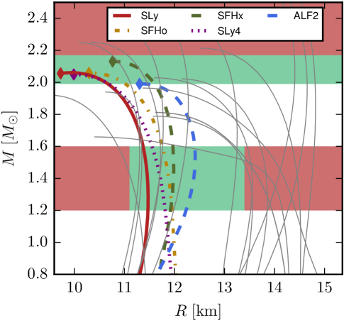
Figure 3: EOS overview including the known constraints on the maximum TOV mass and the NS radius. Realistic EOSs need to fall within the green shaded regions and are outside the $90\%$ confidence intervals in the red areas.

We note that there are a number of potential systematic uncertainties in the presented analysis, which we, however, tried to incorporate and minimize. In general, we have assumed that the kilonova and GRB models are sufficient to generate quantitative conclusions. To be robust against uncertainties, we have employed large systematic error bars for the kilonova analysis as described in Coughlin et al. (2018). In addition, the merger simulations and thereby the determination of ejecta and disk masses may still have large uncertainties because of limited resolution and missing physics, see e.g. Kiuchi et al. (2019). The $\alpha$ and $\xi$ variables encode some of the uncertainty associated with this fact, as they just assume that the simulations are broadly correct up to a scale factor. In addition, while the employed GRB models are relatively simplistic, we have included three different GRB analyses, showing that they, in general, produce consistent results.

Appendix A GW170817 analysis

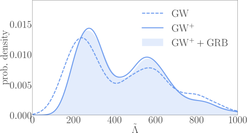
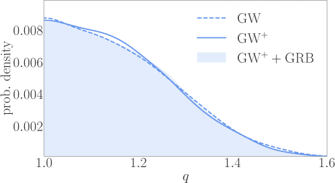
Figure 4: Probability density function for the tidal deformability (top panel) and the mass ratio (bottom panel) obtained by the analysis of GW170817. The dashed line shows the original posterior [denoted as ‘original $GW$’] available at https://dcc.ligo.org/LIGO-P1800370, the solid line shows the posterior using a spectral EOS decomposition as in Carson et al. (2019) [denoted as ’$GW^{+}$’]. The shaded region marks the posterior once we incorporate the viewing angle constraint and assume that the merger was observed under an angle of $22\pm 12$ degree [denoted as ’$GW^{+}+GRB$’. Notice that we use a Kernel Density Estimator (KDE) with bandwidth of $35$ for the tidal deformability and $0.035$ for the mass ratio and that we normalize all distributions to allow a direct comparison. The reduced sample number due to step II and III of our GW analysis (see main text) leads to larger oscillatory behavior for the KDEs.

We build our analysis of GW170817 on the publicly available posteriors released by the LVC and the results of (Carson et al., 2019). We proceed in three steps: (i) we review the original samples, (ii) we restrict the analysis by ensuring that both stars are described by the same EOS, (iii) we restrict the viewing angle based on GRB and afterglow models.

I. Original LIGO posteriors: For GW170817, we use the published results of the LVC (Abbott et al., 2017a, 2019a, 2018, 2019b). In particular, the publicly available posterior samples of Abbott et al. (2019b) provide the starting point for our GW interpretation. We decide to employ the “low spin” assumption, which restricts the rotational frequency of individual NSs so that the individual dimensionless spins are restricted to $\chi\leq 0.05$. This restriction is motivated by the observed BNS in our galaxy where the fastest spinning NS in a BNS system (PSR J1946+2052  (Stovall et al., 2018)) will have a dimensionless spin of $\chi\sim 0.05$ at merger. Thus, we use the samples provided in https://dcc.ligo.org/LIGO-P1800370. The analysis of the follow up LVC results (Abbott et al., 2019a) improves over the initial results of the initial LVC results (Abbott et al., 2017a), as a broader frequency band of $23-2048$ Hz, further improved and recalibrated detector data, more sophisticated waveform models (Dietrich et al., 2019), and the known source location from EM observations have been used (Abbott et al., 2017c).

II. Quasi-universal relations: While (Abbott et al., 2019b) did not make any assumption of the nature of the two merging compact objects, providing a general analysis, it seems natural to assume that the merging objects are two NSs described by the same EOS, an assumption similar to (De et al., 2018; Abbott et al., 2018; Radice & Dai, 2019). Here, we employ the posterior samples of Carson et al. (2019) in which a spectral EOS decomposition is employed. As discussed in the literature, e.g., Chatziioannou et al. (2018); De et al. (2018); Abbott et al. (2019a), enforcing the two objects to be NSs described by the same EOS leads to slightly tighter constrains on the tidal deformability (see the top panel of Fig. 4). We show as a dashed line the original posterior and the solid line marks the posterior using the spectral EOS decomposition. Based on this result, we see that the GW data do not support large tidal deformabilities. This motivates that in the following analysis of the EM counterparts we will restrict the tidal deformabilities to $\tilde{\Lambda}\leq 1100$.

III. The viewing angle: As a last step to restrict the GW posterior samples, we incorporate a viewing angle constraint based on the work of Troja et al. (2019) (note that also other works analyzing GRB170817A and its afterglow can be employed and lead to similar results (Finstad et al., 2018; Mooley et al., 2018)). Troja et al. (2019) finds that the viewing angle of the GRB170817A was $22\pm 6$ degrees. For a conservative estimate, we assume $22\pm 12$ degrees to allow for additional uncertainties. All posterior samples with viewing angles that do not fall inside this interval are discarded. The final result is shown as the shaded region in Fig. 4.

Appendix B Analyzing AT2017gfo

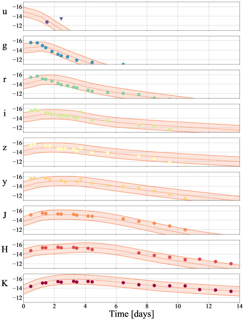
Figure 5: Observational data of AT2017gfo together with the best according to our analysis and the employed kilonova model.

Similar to the analysis of GW170817, we proceed in multiple steps to obtain a posterior distribution of the binary properties of AT2017gfo. For this purpose, we follow and extend the discussion in Coughlin et al. (2018) to which we refer for further details and extensive checks of the underlying algorithms.

I. Modeling AT2017gfo: The observational data (Coughlin et al., 2018; Smartt et al., 2017; Abbott et al., 2017b) (see Fig. 5) are fit with the radiative transfer model of Kasen et al. (2017). The model employs a multi-dimensional Monte Carlo code to solve the multi-wavelength radiation transport equation for an expanding medium. The model allows for the usage of a two component ejecta description. Each component depends parametrically on the ejecta mass $m_{\rm ej}$, the mass fraction of lanthanides $X_{\rm lan}$, and the ejecta velocity $v_{\rm ej}$. These individual parameters will depend on the merger process and the binary parameters. The usage of at least two components is motivated by the presence of different ejecta types. Among the biggest drawbacks of our analysis is the assumption that both components are treated spherically symmetric with a uniform composition. Neglecting mixing of different ejecta types (Rosswog et al., 2017), we add the two separate model components. We have tested the recoveries of the non-spherical models presented in Kasen et al. (2017) using the spherical model. Based on these data, there will be a viewing angle bias in the parameter recoveries here depending on the degree of asymmetry in the ejecta.

We employ a grid with ejecta masses $m_{\rm ej}[M_{\odot}]$ = 0.001, 0.0025, 0.005, 0.0075, 0.01, 0.25, 0.05, and 0.1, ejecta velocities $v_{\rm ej}[c]$ = 0.03, 0.05, 0.1, 0.2, and 0.3, and mass fraction of lanthanides $X_{\rm lan}$ = 0, $10^{-5}$, $10^{-4}$, $10^{-3}$, $10^{-2}$, and $10^{-1}$. In order to draw inferences about generic sources not corresponding to one of these gridpoints, we adapt the approach outlined in Doctor et al. (2017); Pürrer (2014), where GPR is employed to interpolate principal components of gravitational waveforms. The reliability of the method has been tested in Coughlin et al. (2018).

Table 2: Prior choices in the analysis. Intervals indicate a uniform prior, while $\pm$ indicates a Gaussian prior. For the sGRB analyses, we draw the parameters $\tilde{\Lambda}$, $q$, $M_{\rm TOV}$, and $\zeta$ consistent with distributions found from the kilonova analysis.

AT2017gfo		GRB170817A- (Troja et al., 2019)		GRB170817A- (Wu & MacFadyen, 2018)		GRB170817A- (Wang et al., 2019)
parameter	prior	parameter	prior	parameter	prior	parameter	prior
$\tilde{\Lambda}$	[0,1100]	$\tilde{\Lambda}$	KN analysis	$\tilde{\Lambda}$	KN analysis	$\tilde{\Lambda}$	KN analysis
$q$	[1,2]	$q$	KN analysis	$q$	KN analysis	$q$	KN analysis
$M_{\rm TOV}$	[2.0,2.17]	$M_{\rm TOV}$	KN analysis	$M_{\rm TOV}$	KN analysis	$M_{\rm TOV}$	KN analysis
$\log_{10}\alpha$	$[-2,0]$	$\log_{10}E_{0}$	50.30 $\pm$ 0.84	$\log_{10}E_{GRB,50}$	$-$0.81 $\pm$ 0.39	$\log_{10}\sigma$	$[-4,-1]$
$\zeta$	$[0,0.5]$	$\log_{10}\epsilon$	$[-20,0]$	$\log_{10}\epsilon$	$[-20,0]$	$\zeta$	KN analysis
		$\zeta$	KN analysis	$\zeta$	KN analysis

For completeness, we present the lightcurves together with the observational data in Fig. 5. The posterior for the ejecta properties is shown on the left of Fig. 6. The priors for the analysis are given in Table 2. We find that we are able to fit the observational data within the assumed $1$ magnitude uncertainty (Coughlin et al., 2018). We want to point out that although we are able to fit and describe the general X-shooter spectra (Smartt et al., 2017; Pian et al., 2017), the current model is unable to accurately represent observed wavelength specific features (see the discussion in Coughlin et al. (2018)).

II. Relating ejecta properties to the binary parameters:

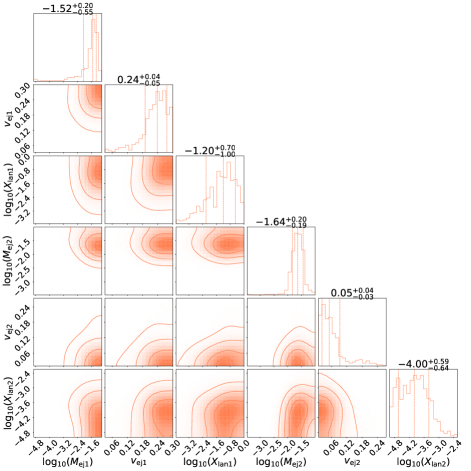
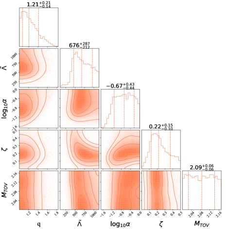
Figure 6: On the left is the posterior distribution of the ejecta properties fitting the observational data presented in Fig. 5. The shown quantities refer to the ejecta mass, velocity, and lanthanide fraction of the first and second ejecta component. On the right is the posterior distribution for our analysis of AT2017gfo. We present posteriors for the mass ratio $q$, the tidal deformability $\tilde{\Lambda}$, the fraction of the first ejecta component related to dynamical ejecta $\alpha$, the fraction of the disk mass ejected as the second component ejecta, and the TOV mass $M_{\rm TOV}$.

To connect the individual ejecta components to the different ejecta mechanisms, we assume that the first ejecta component is proportional to dynamical ejecta, i.e., it gets released during the merger process and is proportional to $m_{\rm dyn}$. The second ejecta component arises from disk winds. We find that constraints on the mass ratio mostly follow from this first assumption, and constraints on the tidal deformability arise mainly from the second ejecta component. While the analysis has velocity and lanthanide fraction priors to make these components physically motivated, in the case where these assumptions are incorrect, the analysis will break down.

With the uncertainty in the modeling of ejecta in numerical relativity simulations and the potential systematic biases due to the missing input physics, we only assume that the dynamical ejecta describes a fraction of the total first component:

$$m_{\rm ej,1}=\frac{1}{\alpha}\ m_{\rm dyn},\qquad v_{\rm ej,1}=v_{\rm dyn}.$$ (6)

To allow for a direct comparison with the GW analysis, we express $m_{\rm dyn}$ in terms of $\tilde{\Lambda}$. This can be achieved by writing the compactnesses of the individual stars as $C_{1,2}=0.371-0.0391\log(\Lambda_{1,2})+0.001056\log(\Lambda_{1,2})^{2}$  (Maselli et al., 2013; Yagi & Yunes, 2017), employing again $\Lambda_{2}=q^{6}\Lambda_{1}$, and using the definition of the tidal deformability

$$\tilde{\Lambda}=\frac{16}{13}\frac{\Lambda_{2}+\Lambda_{1}q^{5}+12\Lambda_{1}q^{4}+12\Lambda_{2}q}{(1+q)^{5}}.$$ (7)

The second ejecta component is related to ejecta arising from disk winds. Long-term simulations find that about $\sim 10-40\%$  (Dessart et al., 2009; Metzger et al., 2008, 2009; Lee et al., 2009; Fernández & Metzger, 2013; Siegel et al., 2014; Just et al., 2015; Metzger & Fernández, 2014; Perego et al., 2014; Martin et al., 2015; Wu et al., 2016; Siegel & Metzger, 2017; Lippuner et al., 2017; Fujibayashi et al., 2017, 2018; Siegel & Metzger, 2018; Metzger et al., 2018; Radice et al., 2018a) of the overall disk mass can be ejected. Thus, it seems plausible to assume

$$m_{\rm ej,2}=\zeta\ m_{\rm disk},$$ (8)

i.e., the disk wind ejecta are overall proportional to the mass of the debris disk surrounding the remnant BH. Knowing that a large fraction of the disk falls into the BH directly after BH formation and that not all matter gets ejected, we restrict $\zeta$ to lie within $\zeta\in[0,0.5]$.

The right part of Fig. 6 shows the findings of our AT2017gfo analysis, which we shortly summarize below: (i) our study favors equal or nearly equal mass systems, where the constraint on the mass ratio mainly arises from the correlation between the first component ejecta and the dynamical ejecta. (ii) $\tilde{\Lambda}$ shows a clear jump at $\tilde{\Lambda}\approx 400$. This constraint arises mainly from the second component ejecta and is related to the disk mass increase for larger values of $\tilde{\Lambda}$. (iii) Only about $20\%$ of the first ejecta component is associated to dynamical ejecta. (iv) About $22\%$ of the disk mass has to be ejected to account for the second ejecta component, which agrees with the disk wind ejecta found in long term numerical relativity simulations. (v) The analysis shows no strong constraint on the maximum allowed TOV mass.

Appendix C Analyzing GRB170817A

In addition to including information about the viewing angle to restrict the GW posteriors (Fig. 4), we will also present a Bayesian parameter estimation for GRB170817A directly. We note that a GRB-GW Bayesian approach was also suggested in Fan et al. (2017).

To relate the GRB properties to the properties of the binary, we employ the typical assumption that the GRB is driven by the accretion of matter from the debris disk onto the BH (Eichler et al., 1989; Paczynski, 1991; Meszaros & Rees, 1992; Narayan et al., 1992; Meszaros, 2006; Lee & Ramirez-Ruiz, 2007; Giacomazzo et al., 2013; Ascenzi et al., 2019) and therefore the energy is proportional to the disk rest mass, i.e.,

$$E_{jet}\propto\ m_{\rm{disk}}.$$ (9)

We note that based on our previous discussion, a fraction of the disk is ejected by disk winds. This part of the original disk cannot drive the GRB, so we set

$$E_{jet}=\varepsilon(m_{\rm disk}-m_{ej,2})=\varepsilon m_{\rm disk}(1-\zeta).$$ (10)

To connect the GRB and kilonova analysis, we reuse the $\zeta$ posterior obtained in the previous subsection. Similarly, we also employ the posterior distributions of $\tilde{\Lambda},q,M_{\rm TOV}$ as priors for our future GRB parameter estimation analysis.

We now briefly describe the three different GRB models/descriptions (Troja et al., 2019; Wu & MacFadyen, 2018; Wang et al., 2019) used in this work.

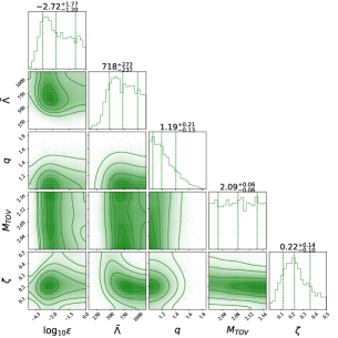
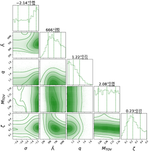
Figure 7: On the left are the posterior distributions for the GRB analysis based on van Eerten et al., 2018. We present constraints on the fraction of the rest mass density of the disk converted to trigger the sGRB, the tidal deformability, the mass ratio and the maximum TOV mass. In the middle are the posterior distributions for the GRB analysis using the GRB energy estimated from Wu & MacFadyen, 2018. On the right are posterior distributions for the GRB analysis using the GRB energy estimated from Wang et al., 2018.

I. The structured GRB-jet model of van Eerten et al (Troja et al., 2019):

Troja et al. (2019) show that the latest observations of the GRB170817A afterglow is consistent with the emergence of a relativistic structured jet (with a jet width $\theta_{c}$ of $4$ degrees) seen at an angle of $\theta_{j}\sim 22\pm 6$ degree from the jet axis. This structured jet model fits well within the range of properties of cosmological sGRBs. Incorporating the Gaussian structured form of the jet as proposed in Troja et al. (2019), the final GRB energy arising from the measured isotropic energy is given by

$$E_{\rm jet}=e^{2\theta_{c}/\theta_{j}}E_{\rm iso}.$$ (11)

According to the analysis of Troja et al. (2019), one obtains $\log_{10}[E_{\rm jet}/{\rm erg}]=50.30^{+0.84}_{-0.57}$. We use this result as an input for Eq. (10) and sample over the final value employing a Gaussian distribution with a width identical to the stated uncertainty in Troja et al. (2019).

The left panel of Fig. 7 shows our results. We find that $\log_{10}\varepsilon\approx-2$, i.e., $1\%$ of the disk rest-mass is converted into GRB energy. This generally agrees with existing theoretical studies (Lee & Ramirez-Ruiz, 2007; Giacomazzo et al., 2013) and increases the confidence in our GRB analysis. Furthermore, we find that the $\tilde{\Lambda}$ estimate and the constraint on the mass ratio shifts to slightly larger values than studying purely AT2017gfo.

II. The GRB model of Wu & MacFadyen (2018): An alternative description of GRB170817A is presented in Wu & MacFadyen (2018). They employ the analytic two-parameter “boosted fireball” model. The model consists of a variety of outflows varying smoothly between a highly collimated ultra-relativistic jet and an isotropic fireball. Developing a synthetic light curve generator, they fit the observational data by performing a Markov-Chain Monte Carlo (MCMC) analysis. Similar to Troja et al. (2019), Wu & MacFadyen (2018) favor a relativistic structured jet. The jet opening angle is $\sim 5$ degrees seen from a viewing angle of $\sim 27$ degree.

The middle panel of Fig. 7 shows our results. The estimated GRB energy is $\log 10_{E_{\rm jet,50}}=-0.81^{+0.26}_{-0.39}$, i.e., more than an order of magnitude below the estimated GRB energy of Troja et al. (2019). Consequently, the estimated value of $\varepsilon$ is smaller. Nevertheless, the constraints on the binary properties and the EOS constraints are in agreement between Troja et al. (2019) and Wu & MacFadyen (2018), i.e., the constraints are robust to the systematic difference in energy estimates.

III. GRB due to the Blanford-Znajek mechanism (Wang et al., 2019):

As a final way to interpret the observed GRB, we follow (Wang et al., 2019). In this model, the energy to launch the GRB, assuming neutrino annihilation as the central engine, requires massive disks masses of the order of $\sim 0.3M_{\odot}$. Such massive disks are in tension with state-of-the-art numerical relativity simulations and disfavor neutrino annihilation as the mechanism responsible for the jet-launch. On the other hand, magnetic energy extraction requires disk masses about one order of magnitude smaller and therefore could act as the central engine for GRB170817A. Following the discussion of Wang et al. (2019), the disk mass necessary to explain the observation of GRB170817A based on the Blanford-Znajek (BZ) mechanism is given by

$$m_{\rm disk}^{\rm BZ}=\underbrace{0.0132M_{\rm\odot}\frac{1}{\mathcal{F}_{\rm GRB}}\frac{E_{\rm GRB}}{10^{51}\rm erg}}_{\sigma}\left(\frac{1+\sqrt{1-\chi_{\rm BH}^{2}}}{\chi_{\rm BH}}\right)^{2}.$$ (12)

In contrast to Wang et al. (2019), we substitute $\frac{0.0132M_{\odot}}{\mathcal{F}_{\rm GRB}}\frac{E_{\rm GRB}}{10^{51}\rm erg}$ by a single parameter $\sigma$ for which we assume a flat prior with $\log_{10}(\sigma)\in[-4,-1]$. Furthermore, we extend the analysis of Wang et al. (2019), who used a flat distribution for the BH spin within $\chi\in[0.6,0.8]$, by employing Eq. (19) to estimate the BH spin, and we substitute the disk mass fits of Radice et al. (2018c) by Eq. (14). As in the previous discussions, we also incorporate the disk wind ejecta via Eq. (10). The right panel of Fig. 7 shows our results. The final results on the tidal deformability, mass ratio, and $M_{\rm TOV}$ are similar to the previous results.

Very recently, Wang et al. (2019) provided constraints on the EOS obtained from a new interpretation of the GRB and its afterglow phase, quoting a constraint of $273<\tilde{\Lambda}<602$. Our tests show that this constraint is highly dependent on the particular choice of $\sigma$ made in Wang et al. (2019). Assuming flat priors on all unknown parameters in Eq. (12) creates a prior peaking at $\sim 10^{-2}$. This prior choice is the driving mechanism for the very tight constraint presented in Wang et al. (2019) and seems in our opinion to be an artifact of the sampling rather than a physical observation.

Appendix D Fits to numerical relativity

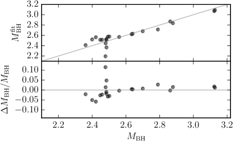
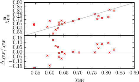
Figure 8: Quality assessment of the phenomenological descriptions of the BH mass (left panels) and BH spin (right panels). The BH quantities are extracted for BNS simulations of the CoRe catalog, a detailed list is presented in Table 3.

Table 3: Overview about the employed numerical relativity dataset to derive the BH remnant fits. Further details are available at http://www.computational-relativity.org. Note that the simulations using data of Bernuzzi et al. (2016) are not identical to the simulations for the same physical configuration available in the CoRe database. The columns refer to: the name of the simulation as stated in the CoRe catalog, the EOS, the total mass $M$, the mass ratio $q$, the tidal deformability $\tilde{\Lambda}$, the references for the simulation and numerical relativity data, the measured BH mass $M_{\rm BH}$ and spin $\chi_{\rm BH}$.

Name	EOS	$M$	$q$	$\tilde{\Lambda}$	Reference	$M_{\rm BH}$	$\chi_{\rm BH}$
BAM:0001:R01	2B	2.70	1.00	127	(Bernuzzi et al., 2015)	2.634	0.785
BAM:0004:R02	ALF2	2.70	1.00	730	(Dietrich et al., 2015)	2.459	0.633
BAM:0005:R01	ALF2	2.75	1.00	658	(Dietrich et al., 2017)	2.493	0.653
BAM:0011:R01	ALF2	3.00	1.00	383	(Dietrich et al., 2018)	2.863	0.760
BAM:0012:R01	ALF2	2.75	1.25	671	(Dietrich et al., 2017)	2.484	0.644
BAM:0016:R01	ALF2	3.20	1.00	246	(Dietrich et al., 2018)	3.128	0.812
BAM:0017:R01	ALF2	2.75	1.50	698	(Dietrich et al., 2017)	2.485	0.629
BAM:0021:R01	ALF2	2.75	1.75	731	(Dietrich et al., 2017)	2.479	0.612
BAM:0036:R01	H4	2.70	1.00	1106	(Dietrich et al., 2015)	2.480	0.621
BAM:0042:R01	H4	2.75	1.00	993	(Dietrich et al., 2018)	2.448	0.592
BAM:0047:R01	H4	3.00	1.00	567	(Dietrich et al., 2018)	2.879	0.773
BAM:0052:R01	H4	3.20	1.00	359	(Dietrich et al., 2018)	3.124	0.828
BAM:0103:R01	SLy	2.70	1.00	388	(Dietrich et al., 2015)	2.484	0.633
BAM:0120:R01	SLy	2.75	1.00	346	(Dietrich & Hinderer, 2017)	2.640	0.769
BAM:0123:R02	SLy	2.70	1.16	490	(Dietrich et al., 2015)	2.502	0.642
BAM:0126:R02	SLy	2.75	1.25	365	(Dietrich et al., 2017)	2.422	0.600
BAM:0128:R01	SLy	2.75	1.50	407	(Dietrich et al., 2017)	2.361	0.544
-	LS220	2.70	1.00	684	(Bernuzzi et al., 2016)	2.40	0.544
-	LS220	2.83	1.04	499	(Bernuzzi et al., 2016)	2.70	0.704
-	SFHo	2.70	1.00	422	(Bernuzzi et al., 2016)	2.56	0.683
-	SFHo	2.83	1.04	312	(Bernuzzi et al., 2016)	2.79	0.808

We now present the fits to numerical relativity we performed which are required for our analyses.

I. Disk mass A crucial ingredient for the analysis in this work and also the recent works of Radice & Dai (2019); Wang et al. (2019) is the estimate of the debris disk mass $m_{\rm disk}$. Here, we revisit the derivation of the phenomenological fit presented in Radice et al. (2018c) and employ their fiducial dataset to derive an updated version of the fit. Figure 15 of Radice et al. (2018c) shows a clear correlation between $m_{\rm disk}$ and the tidal deformability of the binary. We suggest that the reason for this clear and prominent correlation is related to the limited sample of only four EOSs in comparison to the wide range of sampled masses, and the fact that the tidal deformability depends strongly on the total mass of the binary, $\tilde{\Lambda}\sim\left(M_{\rm tot}/R\right)^{-6}$  (De et al., 2018). Already from Fig. 15 of Radice et al. (2018c), one sees that setups with the same EOS (and hence roughly same radii) but different NS masses, lead to different disk masses.

Here we propose an alternative explanation which naturally accounts for the observed phenomenology and scaling with $M_{\rm tot}$. Merger simulations suggest that the disk mass is accumulated primarily through redistribution of matter in the post-merger remnant. Thus, the remnant lifetime prior to collapse is found to strongly correlate with the amount of disk mass (Radice et al., 2018a). Here we suggest that this lifetime is governed to a large degree by $M_{\rm tot}/M_{\rm thr}$, where $M_{\rm thr}$ is the threshold mass above which the merger undergoes a prompt-collapse (on dynamical timescales). Thus $M_{\rm tot}/M_{\rm thr}$ is a measure of the stability of the post-merger remnant, and following the arguments above, should correlate with $m_{\rm disk}$.

We show in Fig. 2 in the main text the correlation between the disk mass and the threshold mass for prompt BH formation, where we estimate the prompt collapse threshold as Bauswein et al. (2013):

$$M_{\rm thr}=\left(2.38-3.606\frac{M_{\rm TOV}}{R_{1.6M_{\odot}}}\right)M_{\rm TOV}.$$ (13)

$M_{\rm TOV}$ denotes the maximum mass of a non-rotating (TOV) NS for a given EOS and $R_{1.6M_{\odot}}$ is the radius of a $1.6M_{\odot}$ star. With the help of Fig. 2 in the main text, it becomes clear that the reduction of the disk mass relates to the stability of the merger remnant and consequently, the disk mass drops abruptly when $M\approx M_{\rm th}$ and the remnant undergoes a prompt-collapse. This naturally explains the location of the turnover in $m_{\rm disk}$.

Based on these observations and the fact that the NS radius can be related to the tidal deformability by $R=\mathcal{M}(\tilde{\Lambda}/a)^{1/6}$ (with the chirp mass $\mathcal{M}$) (De et al., 2018), we conclude that the disk mass is a function of the tidal deformability, the total mass of the system, and the maximum TOV mass $M_{\rm TOV}$. Contrary to Kiuchi et al. (2019), we do not find a strong dependence on the mass ratio and neglect mass ratio effects, when we analysis some of the numerical relativity data of Dietrich et al. (2017). This emphasizes a thoughtful follow-up study using (if possible) different numerical relativity codes to understand the exact dependence of the ejecta and disk mass on the mass ratio of the binary. Therefore, information about the densest part of the EOS, encoded in $M_{\rm TOV}$, and the information at smaller densities, encoded in $\tilde{\Lambda}$ or $R_{1.6M\odot}$, are essential for a reliable description of the disk mass.

To include the dependence of $M_{\rm TOV}$, we also find that fitting $\log_{10}(m_{\rm disk})$ instead of $m_{\rm disk}$ leads to a significant reduction of the fractional error $(m_{\rm disk}-m_{\rm disk}^{\rm fit})/m_{\rm disk}$. We choose the following functional form

$$\log_{10} \left(m_{\rm disk}\left[M_{\rm tot}/M_{\rm thr}\right]\right)=$$

$$\max\left(-3,\ a\left(1+b\tanh\left[\frac{c-M_{\rm tot}/M_{\rm thr}}{d}\right]\right)\right),$$ (14)

with $M_{\rm thr}(M_{\rm TOV},R_{1.6{M_{\odot}}})$ given by Eq. (13). We emphasize that the choice of the exact form of Eq. (14) is arbitrary and other expressions are possible. The free fitting parameters of Eq. (14) are $a=-31.335$, $b=-0.9760$, $c=1.0474$, $d=0.05957$.

The mean absolute error of $m_{\rm disk}$ with respect to the original numerical relativity data is $0.019M_{\odot}$, and we obtain a fractional error of $198\%$ in $m_{\rm disk}$; for comparison, the original fit presented in Radice et al. (2018c) has absolute errors of $0.022M_{\odot}$ and average fractional errors of $749\%$. The large fractional error is caused by a small number of setups with very small disk masses. Fitting the logarithm of the disk mass improves the fit in this region of the parameter space, as already discussed in Coughlin et al. (2018) for the dynamical ejecta. We present the fit as a function of the $M_{\rm tot}/M_{\rm thr}$ in Fig. 2 in the main text and also present the absolute (middle panel) and fractional errors (bottom panel) for Eq. (14) in comparison with the results of Radice et al. (2018c). We point out that in a region around the turning point into prompt collapse scenarios, the absolute and fractional errors of the new fit are noticeable smaller than in the original version.

Finally, since we want to relate information extracted from the disk mass estimates with the GW measurement, we propose to relate the NS radius to the tidal deformability via De et al. (2018)

$$R_{1.6{M_{\odot}}}\simeq\mathcal{M}\left(\frac{\tilde{\Lambda}}{0.0042}\right)^{1/6}.$$ (15)

While informing this relation adds an additional uncertainty, we find that the fitting residuals increase simply to $0.020M_{\odot}$ and $210\%$.

II. Dynamical Ejecta We approximate the mass of the dynamical ejecta by

$$\log_{10}m_{\rm dyn}^{\rm fit}=\left[a\frac{(1-2\ C_{1})M_{1}}{C_{1}}+b\ M_{2}\left(\frac{M_{1}}{M_{2}}\right)^{n}+\frac{d}{2}\right]+[1\leftrightarrow 2],$$ (16)

with $a=-0.0719$, $b=0.2116$, $d=-2.42$, and $n=-2.905$ and $C_{1,2}$ denoting the compactnesses of the individual stars. The absolute uncertainty of the fit, i.e., $m_{\rm dyn}-m_{\rm dyn}^{\rm fit}$ is $7\times 10^{-3}M_{\odot}$. Furthermore, we note that while the fractional error of $\log_{10}m_{\rm dyn}$ is only $36\%$, the fractional error with respect to $m_{\rm dyn}$ is $287\%$ caused by datapoints with very small ejecta masses ($\sim 10^{-4}-10^{-5}M_{\odot}$).

The velocity of the dynamical ejecta is given by

$$v_{\rm dyn}^{\rm fit}=\left[a(1+c\ C_{1})\frac{M_{1}}{M_{2}}+\frac{b}{2}\right]+[1\leftrightarrow 2],$$ (17)

where $a=-0.3090$, $b=0.657$, and $c=-1.879$. The average absolute error of the fit is $\Delta v_{\rm dyn}=0.03$ and the fractional error is $18\%$.

III. BH properties The large set of numerical relativity data publicly released in the CoRe catalog (Dietrich et al., 2018) together with results published in Bernuzzi et al. (2016) allows us to derive phenomenological fits for the BH mass and spin. A detailed list of the employed simulations and the BH properties is presented in Tab. 3. We restrict our consideration to non-spinning NSs, but plan to extend the presented results in the future once a larger set of spinning BNS configurations is available. Furthermore, we consider only cases for which an almost stationary state is reached after BH formation, so that remnant properties can be extracted reliably. Thus, we do not consider setups for which the BH mass increases significantly due to accretion or for which the black hole mass decreases due to insufficient resolution.

Trivially, we find that with an increasing total mass, the final black hole mass and angular momentum increases almost linearly. For unequal mass mergers, $M_{\rm BH}$ and $\chi_{\rm BH}$ decrease. Based on this observation, we propose a functional dependence of $M_{\rm BH}\propto\nu^{\alpha}$ (where $\nu$ refers to the symmetric mass ratio). The coefficient $\alpha$ is chosen to be two, which is motivated by predictions for BBH systems (Healy et al., 2017). Considering the imprint of the EOS, we find that for larger values of $\tilde{\Lambda}$, the final black hole mass decreases, which follows from the observation that the disk mass increases with $\tilde{\Lambda}$. As a simple ansatz, we choose:

$$M_{\rm BH}=a\left(\frac{\nu}{0.25}\right)^{2}\left(M+b\ \frac{\tilde{\Lambda}}{400}\right)$$ (18)

with $a=0.980$ and $b=-0.093$. The mean average absolute error of the fit is $0.065M_{\odot}$ and the fractional error is $2.6\%$.

We find in our dataset that the BH mass and spin are strongly correlated. This motivates the use of a similar functional behavior for the BH spin as for the BH mass. However, we extend Eq. (18) by (i) adding an additional constant, and (ii) incorporating the fact that the dimensionless spin is restricted to be $\chi\leq 1$. The final fitting function is

$$\chi_{\rm BH}=\tanh\left[a\nu^{2}(M+b\ \tilde{\Lambda})+c\right]$$ (19)

with $a=0.537$, $b=-0.185$, and $c=-0.514$. The mean average absolute error of the fit is $0.039$ and the fractional error is $6.1\%$. The remnant property dataset and the corresponding fit results are presented in Fig. 8.

References

- Abbott et al. (2017a) Abbott B. P., et al., 2017a, Phys. Rev. Lett., 119, 161101
- Abbott et al. (2017b) Abbott B. P., et al., 2017b, Astrophys. J., 848, L12
- Abbott et al. (2017c) Abbott B. P., et al., 2017c, Astrophys. J., 848, L13
- Abbott et al. (2017d) Abbott B. P., et al., 2017d, Astrophys. J., 850, L39
- Abbott et al. (2018) Abbott B., et al., 2018, Physical Review Letters, 121
- Abbott et al. (2019a) Abbott B., et al., 2019a, Physical Review X, 9
- Abbott et al. (2019b) Abbott B., et al., 2019b, Physical Review X, 9
- Annala et al. (2018) Annala E., Gorda T., Kurkela A., Vuorinen A., 2018, Phys. Rev. Lett., 120, 172703
- Arcavi et al. (2017) Arcavi I., et al., 2017, Nature, 551, 64
- Ascenzi et al. (2019) Ascenzi S., Lillo N. D., Haster C.-J., Ohme F., Pannarale F., 2019, The Astrophysical Journal, 877, 94
- Bauswein et al. (2013) Bauswein A., Baumgarte T., Janka H. T., 2013, Phys.Rev.Lett., 111, 131101
- Bauswein et al. (2017) Bauswein A., Just O., Janka H.-T., Stergioulas N., 2017, Astrophys. J., 850, L34
- Bernuzzi et al. (2015) Bernuzzi S., Nagar A., Dietrich T., Damour T., 2015, Phys.Rev.Lett., 114, 161103
- Bernuzzi et al. (2016) Bernuzzi S., Radice D., Ott C. D., Roberts L. F., Moesta P., Galeazzi F., 2016, Phys. Rev., D94, 024023
- Carson et al. (2019) Carson Z., Chatziioannou K., Haster C.-J., Yagi K., Yunes N., 2019, Phys. Rev., D99, 083016
- Chatziioannou et al. (2018) Chatziioannou K., Haster C.-J., Zimmerman A., 2018, Phys. Rev., D97, 104036
- Ciolfi & Siegel (2015) Ciolfi R., Siegel D. M., 2015, Astrophys.J., 798, L36
- Coughlin & Dietrich (2019) Coughlin M. W., Dietrich T., 2019, Physical Review D, 100
- Coughlin et al. (2018) Coughlin M. W., et al., 2018, Monthly Notices of the Royal Astronomical Society, 480, 3871
- Coulter et al. (2017) Coulter D. A., et al., 2017, Science
- Dai et al. (2018) Dai L., Venumadhav T., Zackay B., 2018, arXiv: 1806.08793
- De et al. (2018) De S., Finstad D., Lattimer J. M., Brown D. A., Berger E., Biwer C. M., 2018, Phys. Rev. Lett., 121, 091102
- Dessart et al. (2009) Dessart L., Ott C., Burrows A., Rosswog S., Livne E., 2009, Astrophys.J., 690, 1681
- Dietrich & Hinderer (2017) Dietrich T., Hinderer T., 2017, Phys. Rev., D95, 124006
- Dietrich & Ujevic (2017) Dietrich T., Ujevic M., 2017, Class. Quant. Grav., 34, 105014
- Dietrich et al. (2015) Dietrich T., Bernuzzi S., Ujevic M., Brügmann B., 2015, Phys. Rev., D91, 124041
- Dietrich et al. (2017) Dietrich T., Ujevic M., Tichy W., Bernuzzi S., Brügmann B., 2017, Phys. Rev., D95, 024029
- Dietrich et al. (2018) Dietrich T., et al., 2018, arXiv: 1806.01625
- Dietrich et al. (2019) Dietrich T., et al., 2019, Physical Review D, 99
- Doctor et al. (2017) Doctor Z., Farr B., Holz D. E., Pürrer M., 2017, Phys. Rev., D96, 123011
- Dudi et al. (2018) Dudi R., Pannarale F., Dietrich T., Hannam M., Bernuzzi S., Ohme F., Brügmann B., 2018, Phys. Rev., D98, 084061
- Eichler et al. (1989) Eichler D., Livio M., Piran T., Schramm D. N., 1989, Nature, 340, 126
- Fan et al. (2017) Fan X., Messenger C., Heng I. S., 2017, Phys. Rev. Lett., 119, 181102
- Fernández & Metzger (2013) Fernández R., Metzger B. D., 2013, Mon. Not. Roy. Astron. Soc., 435, 502
- Finstad et al. (2018) Finstad D., De S., Brown D. A., Berger E., Biwer C. M., 2018, Astrophys. J., 860, L2
- Fujibayashi et al. (2017) Fujibayashi S., Sekiguchi Y., Kiuchi K., Shibata M., 2017, Astrophys. J., 846, 114
- Fujibayashi et al. (2018) Fujibayashi S., Kiuchi K., Nishimura N., Sekiguchi Y., Shibata M., 2018, Astrophys. J., 860, 64
- Giacomazzo et al. (2013) Giacomazzo B., Perna R., Rezzolla L., Troja E., Lazzati D., 2013, Astrophys. J., 762, L18
- Healy et al. (2017) Healy J., Lousto C. O., Zlochower Y., 2017, Phys. Rev., D96, 024031
- Hinderer et al. (2019) Hinderer T., et al., 2019, Physical Review D, 100
- Just et al. (2015) Just O., Bauswein A., Pulpillo R. A., Goriely S., Janka H. T., 2015, Mon. Not. Roy. Astron. Soc., 448, 541
- Kasen et al. (2017) Kasen D., Metzger B., Barnes J., Quataert E., Ramirez-Ruiz E., 2017, Nature, 10.1038/nature24453
- Kiuchi et al. (2019) Kiuchi K., Kyutoku K., Shibata M., Taniguchi K., 2019, Astrophys. J., 876, L31
- Kohri et al. (2005) Kohri K., Narayan R., Piran T., 2005, Astrophys. J., 629, 341
- Lee & Ramirez-Ruiz (2007) Lee W. H., Ramirez-Ruiz E., 2007, New J. Phys., 9, 17
- Lee et al. (2009) Lee W. H., Ramirez-Ruiz E., Diego-Lopez-Camara 2009, Astrophys.J., 699, L93
- Lippuner et al. (2017) Lippuner J., Fernández R., Roberts L. F., Foucart F., Kasen D., Metzger B. D., Ott C. D., 2017, Mon. Not. Roy. Astron. Soc., 472, 904
- Lipunov et al. (2017) Lipunov V. M., et al., 2017, Astrophys. J., 850, L1
- Margalit & Metzger (2017) Margalit B., Metzger B. D., 2017, Astrophys. J., 850, L19
- Martin et al. (2015) Martin D., Perego A., Arcones A., Thielemann F.-K., Korobkin O., Rosswog S., 2015, Astrophys. J., 813, 2
- Maselli et al. (2013) Maselli A., Cardoso V., Ferrari V., Gualtieri L., Pani P., 2013, Phys. Rev., D88, 023007
- Meszaros (2006) Meszaros P., 2006, Rept. Prog. Phys., 69, 2259
- Meszaros & Rees (1992) Meszaros P., Rees M. J., 1992, Astrophys. J., 397, 570
- Metzger & Fernández (2014) Metzger B. D., Fernández R., 2014, Mon.Not.Roy.Astron.Soc., 441, 3444
- Metzger et al. (2008) Metzger B., Piro A., Quataert E., 2008, Mon.Not.Roy.Astron.Soc., 390, 781
- Metzger et al. (2009) Metzger B. D., Piro A. L., Quataert E., 2009, Mon. Not. Roy. Astron. Soc., 396, 304
- Metzger et al. (2018) Metzger B. D., Thompson T. A., Quataert E., 2018, Astrophys. J., 856, 101
- Mooley et al. (2018) Mooley K. P., et al., 2018, Nature, 554, 207
- Most et al. (2018) Most E. R., Weih L. R., Rezzolla L., Schaffner-Bielich J., 2018, Phys. Rev. Lett., 120, 261103
- Narayan et al. (1992) Narayan R., Paczynski B., Piran T., 1992, Astrophys. J., 395, L83
- Paczynski (1991) Paczynski B., 1991, Acta Astron., 41, 257
- Perego et al. (2014) Perego A., Rosswog S., Cabezon R., Korobkin O., Kaeppeli R., et al., 2014, Mon.Not.Roy.Astron.Soc., 443, 3134
- Pian et al. (2017) Pian E., et al., 2017, Nature
- Pürrer (2014) Pürrer M., 2014, Class. Quant. Grav., 31, 195010
- Radice & Dai (2019) Radice D., Dai L., 2019, The European Physical Journal A, 55
- Radice et al. (2018a) Radice D., Perego A., Bernuzzi S., Zhang B., 2018a, arXiv:1803.10865
- Radice et al. (2018b) Radice D., Perego A., Zappa F., Bernuzzi S., 2018b, Astrophys. J., 852, L29
- Radice et al. (2018c) Radice D., Perego A., Hotokezaka K., Fromm S. A., Bernuzzi S., Roberts L. F., 2018c, The Astrophysical Journal, 869, 130
- Rezzolla & Kumar (2015) Rezzolla L., Kumar P., 2015, Astrophys. J., 802, 95
- Rezzolla et al. (2018) Rezzolla L., Most E. R., Weih L. R., 2018, Astrophys. J., 852, L25
- Rosswog et al. (2017) Rosswog S., Feindt U., Korobkin O., Wu M. R., Sollerman J., Goobar A., Martinez-Pinedo G., 2017, Class. Quant. Grav., 34, 104001
- Ruiz et al. (2018) Ruiz M., Shapiro S. L., Tsokaros A., 2018, Phys. Rev., D97, 021501
- Samajdar & Dietrich (2018) Samajdar A., Dietrich T., 2018, Physical Review D, 98
- Shibata et al. (2017) Shibata M., Fujibayashi S., Hotokezaka K., Kiuchi K., Kyutoku K., Sekiguchi Y., Tanaka M., 2017, Phys. Rev., D96, 123012
- Siegel & Metzger (2017) Siegel D. M., Metzger B. D., 2017, Phys. Rev. Lett., 119, 231102
- Siegel & Metzger (2018) Siegel D. M., Metzger B. D., 2018, Astrophys. J., 858, 52
- Siegel et al. (2014) Siegel D. M., Ciolfi R., Rezzolla L., 2014, Astrophys. J., 785, L6
- Smartt et al. (2017) Smartt S. J., et al., 2017, Nature, 10.1038/nature24303
- Soares-Santos et al. (2017) Soares-Santos M., et al., 2017, Astrophys. J., 848, L16
- Stovall et al. (2018) Stovall K., et al., 2018, Astrophys. J., 854, L22
- Surman et al. (2006) Surman R., McLaughlin G. C., Hix W. R., 2006, Astrophys. J., 643, 1057
- Tanvir et al. (2017) Tanvir N. R., et al., 2017, Astrophys. J., 848, L27
- Troja et al. (2019) Troja E., et al., 2019, Monthly Notices of the Royal Astronomical Society
- Valenti et al. (2017) Valenti S., et al., 2017, Astrophys. J., 848, L24
- Wang et al. (2019) Wang Y.-Z., et al., 2019, The Astrophysical Journal, 877, 2
- Wu & MacFadyen (2018) Wu Y., MacFadyen A., 2018, arXiv:1809.06843
- Wu et al. (2016) Wu M.-R., Fernández R., Martínez-Pinedo G., Metzger B. D., 2016, Mon. Not. Roy. Astron. Soc., 463, 2323
- Yagi & Yunes (2017) Yagi K., Yunes N., 2017, Phys. Rept., 681, 1