Divergence Measures Estimation and Its Asymptotic Normality Theory in the discrete case

Abstract.

In this paper we provide the asymptotic theory of the general of $\phi$-divergences measures, which includes the most common divergence measures: Renyi and Tsallis families and the Kullback-Leibler measure. We are interested in divergence measures in the discrete case. One sided and two-sided statistical tests are derived as well as symmetrized estimators. Almost sure rates of convergence and asymptotic normality theorem are obtained in the general case, and next particularized for the Renyi and Tsallis families and for the Kullback-Leibler measure as well. Our theorical results are validated by simulations.

1. Introduction

1.1. Motivations

In this paper, we study the convergence of $\phi-$divergence measure estimator for empirical discrete probability distributions supported on a finite set.

Let throughout the following $\mathcal{X}=\{c_{1},c_{2},\cdots,c_{r}\}\,(r\geq 2)$ be a finite countable space. The probability distributions on $\mathcal{X}$ are finite dimensional vectors p in

$$\mathcal{P}(\mathcal{X})=\left\{\textbf{p}=(p_{c})_{c\in\mathcal{X}}:p_{c}\geq 0,\,\forall c\in\mathcal{X}\ \ \text{and}\ \ \sum_{c\in\mathcal{X}}p_{c}=1\right\}.$$

A divergence measure on $\mathcal{P}(\mathcal{X})$ is a function

(1.1)

$$\mathcal{D}:$$

such that $\mathcal{D}(\textbf{p},\textbf{p})=0$ for any p such that $(\textbf{p},\textbf{p})$ in the domain of application of $\mathcal{D}$.

The function $\mathcal{D}$ is not necessarily a mapping. And if it is, it is not always symmetrical and it does neither have to be a metric. In lack of symmetry, the following more general notation is more appropriate :

(1.2)

$$\mathcal{D}:$$

,

where $\mathcal{P}_{1}(\mathcal{X})$ and $\mathcal{P}_{2}(\mathcal{X})$ are two families of probability distributions on $\mathcal{X}$, not necessarily the same. To better explain our concern, let us introduce some of the most celebrated divergence measures.

Let $(\textbf{p},\textbf{q})\in\mathcal{P}(\mathcal{X})\times\mathcal{P}(\mathcal{X})$ with $\mathcal{X}=\{c_{1},c_{2},\cdots,c_{r}\}$, and let $X$ and $Y$ two randoms variables such that

$$\mathbb{P}(X=c_{j})=p_{j},\ \ \text{and}\ \ \mathbb{P}(Y=c_{j})=q_{j},\ \ j\in\{1,\cdots,r\}.$$

and set $\textbf{p}=(p_{1},\cdots,p_{r})^{t}$ and $\textbf{q}=(q_{1},\cdots,q_{r})^{t}$.

The four most popular divergence are :

(1) The $L_{2}^{2}$-divergence measure :

(1.3) $$\mathcal{D}_{L_{2}}(\textbf{p},\textbf{q})=\sum_{j=1}^{r}(p_{j}-q_{j})^{2}.$$

(2) The family of Renyi’s divergence measures indexed by $\alpha\neq 1$, $\alpha>0$, known under the name of Renyi-$\alpha$ :

(1.4) $$\mathcal{D}_{R,\alpha}(\textbf{p},\textbf{q})=\frac{1}{\alpha-1}\log\left(\sum_{j=1}^{r}p_{j}^{\alpha}q_{j}^{1-\alpha}\right).$$

(3) The family of Tsallis divergence measures indexed by $\alpha\neq 1$, $\alpha>0$, also known under the name of Tsallis-$\alpha$ :

(1.5) $$\mathcal{D}_{T,\alpha}(\textbf{p},\textbf{q})=\frac{1}{\alpha-1}\left(\sum_{j=1}^{r}p_{j}^{\alpha}q_{j}^{1-\alpha}-1\right);$$

(4) The Kulback-Leibler divergence measure

(1.6) $$\mathcal{D}_{KL}(\textbf{p},\textbf{q})=\sum_{j=1}^{r}p_{j}\log(p_{j}/q_{j}).$$

The latter, the Kullback-Leibler divergence measure, may be interpreted as a limit case of both the Renyi’s family and the Tsallis’ one by letting $\alpha\rightarrow 1$. As well, for $\alpha$ near 1, the Tsallis family may be seen as derived from $\mathcal{D}_{R,\alpha}(\textbf{p},\textbf{q})$ based on the first order expansion of the logarithm function in the neighborhood of the unity. Here for ease of notation we refer the notation log as the natural logarithm

From this small sample of divergence measures, we may give the following remarks :

For both the Renyi and the Tsallis families, we may have computation problems. So without loss of generality, suppose

(1.7) $$\ \ \ p_{j}>0\ \ \text{and}\ \ q_{j}>0,\ \ \forall j\in D=\{1,2,\cdots,r\}\ \ \ \ \ (\textbf{BD})$$

If Assumption (1.7) holds, we do not have to worry about summation problems, especially for Tsallis, Renyi and Kulback-Leibler measures, in the computations arising in estimation theories. This explains why Assumption (1.7) is systematically used in a great number of works in that topic, for example, in Singh and Poczos (2014), Krishnamurthy et al. (2014), Hall (1987), and recently in Bâ et al. (2018) to cite a few.

It is clear from the very form of these divergence measures that we do not have symmetry, unless for the special case where $\alpha=1/2$. So we define the following symetric version of divergence measures

$$\mathcal{D}^{(s)}(\textbf{p},\textbf{q})=\frac{\mathcal{D}(\textbf{p},\textbf{q})+\mathcal{D}(\textbf{q},\textbf{p})}{2}$$

provided that $\mathcal{D}(\textbf{p},\textbf{q})$ and $\mathcal{D}(\textbf{q},\textbf{p})$ are finite.

Both families are build on the following summation

$$\mathcal{S}_{\alpha}(\textbf{p},\textbf{q})=\sum_{j\in D}p_{j}^{\alpha}q_{j}^{1-\alpha},\ \ \text{with}\ \ \alpha\neq 1,\ \ \alpha>0.$$

Although we are focusing on the aforementioned divergence measures in this paper, it is worth mentioning that there exist quite a few number of them. Let us cite for example the ones named after : Ali-Silvey or $f$-divergence Topsoe (2000), Cauchy-Schwarz, Jeffrey divergence (see Evren (2012)), Chernoff (See Evren (2012)) , Jensen-Shannon (See Evren (2012)). According to Cichocki and Amari (2010), there is more than a dozen of different divergence measures in the literature.

Before coming back to our divergence measures estimation of interest, we want to highlight some important applications of them. Indeed, divergence has proven to be useful in applications. Let us cite a few of them :

(a) They heavily intervene in Information Theory and recently in Machine Learning.

(b) They have been used as similarity measures in image registration or multimedia classification (see Moreno et al. (2004)).

(c) They are also used as loss functions in evaluating and optimizing the performance of density estimation methods (see Hall (1987)).

(d) Divergence estimates can also be used to determine sample sizes required to achieve given performance levels in hypothesis testing.

(e) There has been a growing interest in applying divergence to various fields of science and engineering for the purpose of estimation, classification, etc. (See Bhattacharya (1967), Liu and Shum (2003)).

(f) Divergence also plays a central role in the frame of large deviations results including the asymptotic rate of decrease of error probability in binary hypothesis testing problems.

(g) The estimation of divergence between the samples drawn from unknown distributions gauges the distance between those distributions. Divergence estimates can then be used in clustering and in particular for deciding whether the samples come from the same distribution by comparing the estimate to a threshold.

(h) Divergence gauges how differently two random variables are distributed and it provides a useful measure of discrepancy between distributions. In the frame of information theory, the key role of divergence is well known.

The reader may find more applications and descriptions in the following papers : Kullback and Leibler (1951),Fukunaga and Hayes (1989), Cardoso (1997), Ojala et al. (1996), Hastie and Tibshirani (1998), Moreno et al. (2004),MacKay (2003).

In the next subsection, we describe the frame in which we place the estimation problems we deal in this paper.

1.2. Statistical Estimations

The divergence measures may be applied to two statistical problems among others.

(A) First, it may be used as a fitting problem as described here. Let $X_{1},X_{2},\cdots$ a sample of replications of $X$ with an unknown probability distribution p and we want to test the hypothesis that p is equal to a known and fixed probability $\textbf{p}_{0}.$ Theoretically, we can answer this question by estimating a divergence measure $\mathcal{D}(\textbf{p},\textbf{p}_{0})$ by a plug-in estimator $\mathcal{D}(\widehat{\textbf{p}}_{n},\textbf{p})$ where, for each $n\geq 1$, p is replaced by an estimator $\widehat{\textbf{p}}_{n}$ of the probability law, which is based on sample $X_{1}$, $X_{2}$, …, $X_{n}$, to be precised.

From there establishing an asymptotic theory of $\Delta_{n}=\mathcal{D}(\widehat{\textbf{p}}_{n},\textbf{p}_{0})-\mathcal{D}(\textbf{p},\textbf{p}_{0})$ is thought to be necessary to conclude.

(B) Next, it may be used as tool of comparing for two distributions. We may have two samples and wonder whether they come from the same probability distribution. Here, we also may two different cases.

(B1) In the first, we have two independent samples $X_{1},X_{2},....$ and $Y_{1},Y_{2},....$ respectively from a random variable $X$ and $Y$ according the probability distributions p and q. Here the estimated divergence $\mathcal{D}(\widehat{\textbf{p}}_{n},\widehat{\textbf{q}}_{m})$, where $n$ and $m$ are the sizes of the available samples, is the natural estimator of $\mathcal{D}(\textbf{p},\textbf{q})$ on which depends the statistical test of the hypothesis : $\textbf{p}=\textbf{q}$.

(B2) But the data may also be paired $(X,Y)$, $(X_{1},Y_{2}),(X_{2},Y_{2}),...,$ that is $X_{i}$ and $Y_{i}$ are measurements of the same case $i=1,2,...$ In such a situation, testing the equality of the margins $\textbf{p}_{X}=\textbf{p}_{Y}$ should be based on an estimator $\widehat{\textbf{p}}_{X,Y}^{(n)}$ of the joint probability law of the couple $(X,Y)$ based of the paired observations $(X_{i},Y_{i})$, $i=1,2,\ldots,n$.

We did not encounter the approach (B2) in the literature. In the (B1) approach, almost all the papers used the same sample size, at the exception of Poczos and Jeff (2011), for the double-size estimation problem. In our view, the study case should rely on the available data so that using the same sample size may lead to a loss of information. To apply their method, one should take the minimum of the two sizes and then loose information. We suggest to come back to a general case and then study the asymptotic theory of $\mathcal{D}(\widehat{\textbf{p}}_{n},\widehat{\textbf{q}}_{m})$ based on samples $X_{1},X_{2},..,X_{n}.$ and $Y_{1},Y_{2},...,Y_{m}$. In this paper, we will systematically use arbitrary samples sizes.

1.3. Previous work

In the context of the situation (B1), there are several papers dealing with the estimation of the divergence measures. As we are concerned in this paper by the weak laws of the estimators, our review on that problematic did not return significant things. Instead, the literature presented us many kinds of results on almost-sure efficiency of the estimation, with rates of convergences and laws of the iterated logarithm, $L^{p}$ ($p=1,2$) convergences, etc. To be precise, Dhakher et al. (2016) used recent techniques based on functional empirical process to provide a series of interesting rates of convergence of the estimators in the case of one-sided approach for the class de Renyi, Tsallis, Kullback-Leibler to cite a few. Unfortunately, the authors did not address the problem of integrability, taking that the divergence measures are finite. Although the results should be correct under the boundedness assumption (1.7) (BD) we described earlier, a new formulation in that frame would be welcome.

In the context of the situation (B1), we may cite first the works of Krishnamurthy et al. (2014) and Singh and Poczos (2014). They both used divergence measures based on probability density functions and concentrated of Renyi-$\alpha$, Tsallis-$\alpha$ and Kullback-Leibler.

Specifically, Krishnamurthy et al. (2014) defined Reyni and Tsallis estimators by correcting the plug-in estimator and established that, as long as $\mathcal{D}_{R,\alpha}(\textbf{p},\textbf{q})\geq c$ and $\mathcal{D}_{T,\alpha}(\textbf{p},\textbf{q})\geq c$, for some constant $c>0$, then

$$\mathbb{E}\left|\mathcal{D}_{R,\alpha}(\widehat{\textbf{p}}_{n},\widehat{\textbf{q}}_{n})-\mathcal{D}_{R,\alpha}(\textbf{p},\textbf{q})\right|\leq c\left(n^{-1/2}+n^{-\frac{3s}{2s+d}}\right)$$

and

$$\mathbb{E}\left|\mathcal{D}_{T,\alpha}(\widehat{\textbf{p}}_{n},\widehat{\textbf{q}}_{n})-\mathcal{D}_{T,\alpha}(\textbf{p},\textbf{q})\right|\leq c\left(n^{-1/2}+n^{-\frac{3s}{2s+d}}\right),$$

Poczos and Jeff (2011) used a $k-$nearest-neighbor approach to prove that if $|\alpha-1|<k$, ($\alpha\neq 1)$ then

$$\lim_{n,m\rightarrow\infty}\mathbb{E}\left[\mathcal{D}_{T,\alpha}(\widehat{\textbf{p}}_{n},\widehat{\textbf{q}}_{m})-\mathcal{D}_{T,\alpha}(\textbf{p},\textbf{q})\right]^{2}=0$$

and

$$\lim_{n,m\rightarrow\infty}\mathbb{E}\left(\mathcal{D}_{R,\alpha}(\widehat{\textbf{p}}_{n},\widehat{\textbf{q}}_{m})\right)=\mathcal{D}_{R,\alpha}(\textbf{p},\textbf{q}).$$

There has been recent interest in deriving convergence rates for divergence estimators Moon and Hero (2014)-Krishnamurthy et al. (2014). The rates are typically derived in terms of smoothness $s$ of the densities :

The estimator of Liu et al. (2012) converges at rate $n^{-\frac{s}{s+d}}$, achieving the parametric rate when $s>d$.

Similarly, Sricharan et al. (2012) show that when $s>d$ a $k$-nearest-neighbor style estimator achieves rate $n^{-2/d}$ (in absolute error) ignoring logarithmic factors. In a follow up work, the authors improve this result to $O(n^{-1/2})$ using an ensemble of weak estimators, but they require $s>d$ orders of smoothness.

Singh and Poczos (2014) provided an estimator for Rényi$-\alpha$ divergences as well as general density functionals that uses a mirror image kernel density estimator. They obtained exponential inequalities for the deviation of the estimators from the true value.

Kallberg and Seleznjev (2012) studied an $\varepsilon-$nearest neighbor estimator for the $L_{2}-$divergence that enjoys the same rate of convergence as the projection-based estimator of Krishnamurthy et al. (2014).

1.4. Main contributions

Our main contribution may be summurized as follows, for data sampled from one or two unknown random variables, we derive almost sure convergency and central limit theorems for empirical $\phi-$ divergences. We will focus on divergence measures between discrete probability distribution. As well, our results applied to the approaches (A) and (B1) defined above. As a consequence, we estimate divergence measures by their plug-in counterparts, meaning that we replace the probability mass function (p.m.f.) in the expression of the divergence measure by a nonparametric estimator of the p.m.f.’s.

We also wish to get first general laws for an arbitrary functional of the form

(1.8) $$J(\textbf{p},\textbf{q})=\sum_{j\in D}\phi(p_{j},q_{j}),$$

where $\phi:(0,1)^{2}\rightarrow\mathbb{R}$ is a twice continously differentiable function. The results on the functional $J(\textbf{p},\textbf{q})$, which is also known under the name of $\phi$-divergence, will lead to those on the particular cases of the Tsallis and Kullback-Leibler measures.

1.5. Overview of the paper

The rest of the paper is organized as follows. In Subsection 2.1, we define estimators of the p.m.f. $p_{j}$ and $q_{j}$ based on i.i.d. samples according respectively to p and q. In Section 3, we will give our foul results for functional $J(\textbf{p},\textbf{q})$ both one sided and two-sided approaches. In Section 4, we will particularize the results for specific measures we already described. Section 5 provides the proofs and in Section 6 we present some simulations confirming our results. Finally in Section 7, we conclude.

2. Empirical $\phi-$ divergence

2.1. Notations and main results

Before we state the main results we need a few definitions. Let $X$ and $Y$ two randoms variables defined on the probability distributions $(\mathcal{X},\mathcal{A},\mathbb{P})$ with $\mathcal{X}=\{c_{1},c_{2},\cdots,c_{r}\}$ and $\mathbf{p}=(p_{j})_{1\leq j\leq r}$ and $\mathbf{q}=(q_{j})_{1\leq j\leq r}$ two discrete probability distributions on $\mathcal{X}$ such that, for any $j\in D=\{1,2,\cdots,r\}$

$$p_{j}=\mathbb{P}(X=c_{j})\ \ \text{and}\ \ q_{j}=\mathbb{P}(Y=c_{j}).$$

We suppose that (1.7) is satisfied that is $\forall\,j\in D,\ \ p_{j}>0\ \ \text{and}\ \ q_{j}>0.$

Define the empirical probability distribution generated by i.i.d. random variables $X_{1},\cdots,X_{n}$ from the probability distribution p as

(2.1) $$\widehat{\textbf{p}}_{n}=(\widehat{p}_{n}^{c})_{c\in\mathcal{X}},\ \ \text{where}\ \ \widehat{p}_{n}^{c_{j}} = \frac{1}{n}\sum_{i=1}^{n}1_{c_{j}}(X_{i})$$

where $1_{c_{j}}(X_{i})=\begin{cases}1\ \ \text{if}\ \ X_{i}=c_{j}\\ 0\ \ \text{otherwise}\end{cases}$ for any $j\in\{1,\cdots,r\}$.

$\widehat{\textbf{q}}_{m}$ is defined in the same way by $Y_{1},\cdots,Y_{m}\stackrel{{\scriptstyle i.i.d.}}{{\sim}}\textbf{q}$ that is

(2.2) $$\widehat{\textbf{q}}_{m}=(\widehat{q}_{m}^{c})_{c\in\mathcal{X}},\ \ \text{where}\ \ \widehat{q}_{m}^{c_{j}}=\frac{1}{m}\sum_{i=1}^{m}1_{c_{j}}(Y_{i}),$$

2.2. $\phi$-divergence measure

Definition 1.

The $\phi$-divergence between the two probability distributions p and q is given by

(2.3) $$J(\textbf{p},\textbf{q})=\sum_{j\in D}\phi(p_{j},q_{j})$$

where $\phi:[0,1]^{2}\rightarrow\mathbb{R}$ is a measurable function having continuous second order partial derivatives.

The results on the functional $J(\textbf{p},\textbf{q})$ will lead to those on the particular cases of the Renyi, Tsallis, and Kullback-Leibler measures.

Based on (2.1) and (2.2), we will use the following empirical $\phi$-divergences.

$$J(\widehat{\textbf{p}}_{n},\textbf{q}) = \sum_{j\in D}\phi(\widehat{p}_{n}^{c_{j}},q_{j}),\text{\ \ \ \ }J(\textbf{p},\widehat{\textbf{q}}_{m})=\sum_{j\in D}\phi(p_{j},\widehat{q}_{m}^{c_{j}}),$$

  and $$J(\widehat{\textbf{p}}_{n},\widehat{\textbf{q}}_{m})=\sum_{j\in D}\phi(\widehat{p}_{n}^{c_{j}},\widehat{q}_{m}^{c_{j}}).$$

Set

(2.4) $$a_{n} = \sup_{j\in D}|\widehat{p}_{n}^{c_{j}}-p_{j}|,\ \ \ \ b_{m}=\sup_{j\in D}|\widehat{q}_{m}^{c_{j}}-q_{j}|,$$

and $$c_{n,m}=\max(a_{n},b_{m}).$$

Denote

$$\phi_{1}^{(1)}(s,t)=\frac{\partial\phi}{\partial s}(s,t),\text{ }\phi_{2}^{(1)}(s,t)=\frac{\partial\phi}{\partial t}(s,t)$$

and

$$\phi_{1}^{(2)}(s,t)=\frac{\partial^{2}\phi}{\partial s^{2}}(s,t),\text{ }\phi_{2}^{(2)}(s,t)=\frac{\partial^{2}\phi}{\partial t^{2}}(s,t),\text{ }\phi_{1,2}^{(2)}(s,t)=\phi_{2,1}^{(2)}(s,t)=\frac{\partial^{2}\phi}{\partial s\partial t}(s,t).$$

Set

(2.5) $$A_{1,p} = \sum_{j\in D}|\phi_{1}^{(1)}(p_{j},q_{j})|,\ \ \ A_{2,q}=\sum_{j\in D}|\phi_{2}^{(1)}(p_{j},q_{j})|$$

(2.6) $$A_{3,q} = \sum_{j\in D}|\phi_{1}^{(1)}(q_{j},p_{j})|,\ \ \text{and}\ \ A_{4,p}=\sum_{j\in D}|\phi_{2}^{(1)}(q_{j},p_{j})|.$$

3. Statements of the main results

3.1. Main results

Here are our main results. The first concerns the almost sure efficiency of the estimators.

Theorem 1.

Let p and q two probability distributions and $\widehat{\textbf{p}}_{n}$ and $\widehat{\textbf{q}}_{m}$ be generated by i.i.d. samples $X_{1},\cdots,X_{n}$ and $Y_{1},\cdots,Y_{m}$ according respectively to p and q and given by (2.1) and (2.2), $(BD)$ (1.7) be satisfied. Then the following asymptotic results hold

• One sample

  (3.1) $$\limsup_{n\rightarrow+\infty}\frac{|J(\widehat{\textbf{p}}_{n},\textbf{q})-J(\textbf{p},\textbf{q})|}{a_{n}}\leq A_{1,p},\ \ \text{a.s.}$$

  (3.2) $$\limsup_{m\rightarrow+\infty}\frac{\left|J(\textbf{p},\widehat{\textbf{q}}_{m})-J(\textbf{p},\textbf{q})\right|}{b_{m}}\leq A_{2,q},\ \ \text{a.s.}$$

• Two samples :

  (3.3) $$\limsup_{(n,m)\rightarrow(+\infty,+\infty)}\frac{\left|J(\widehat{\textbf{p}}_{n},\widehat{\textbf{q}}_{m})-J(\textbf{p},\textbf{q})\right|}{c_{n,m}}\leq A_{1,p}+A_{2,q}\text{\ \ a.s.}$$

where $a_{n}$, $b_{m}$ and $c_{n,m}$ are as in (2.4) and $A_{1,p}$ and $A_{2,q}$ as in (2.5).

The second concerns the asymptotic normality of the estimators.

Let

$$V_{1,p}=\sum_{j\in D}p_{j}(1-p_{j})(\phi_{1}^{(1)}(p_{j},q_{j}))^{2}-2\sum_{(i,j)\in D^{2},\,i\neq j}p_{i}p_{j}\phi_{1}^{(1)}(p_{i},q_{i})\phi_{1}^{(1)}(p_{j},q_{j})$$

and

$$V_{2,q}=\sum_{j\in D}q_{j}(1-q_{j})(\phi_{2}^{(1)}(p_{j},q_{j}))^{2}-2\sum_{(i,j)\in D^{2},\ i\neq j}q_{i}q_{j}\phi_{2}^{(1)}(p_{i},q_{i})\phi_{2}^{(1)}(p_{j},q_{j})$$

Theorem 2.

Under the same assumptions as in Theorem 1, the following central limit theorems hold.

• One sample : as $n\rightarrow+\infty$,

  (3.4) $$\sqrt{n}(J(\widehat{\textbf{p}}_{n},\textbf{q})-J(\textbf{p},\textbf{q}))\stackrel{{\scriptstyle\mathcal{D}}}{{\rightsquigarrow}}\mathcal{N}\left(0,V_{1,p}\right),$$

  (3.5) $$\sqrt{m}(J(\textbf{p},\widehat{\textbf{q}}_{m})-J(\textbf{p},\textbf{q}))\stackrel{{\scriptstyle\mathcal{D}}}{{\rightsquigarrow}}\mathcal{N}\left(0,V_{2,q}\right),$$

• Two samples : for $(n,m)\rightarrow(+\infty,+\infty)$ and $nm/(n+m)\rightarrow\gamma\in(0,1)$,

  (3.6) $$\left(\frac{nm}{mV_{1,p}+nV_{2,q}}\right)^{1/2}\left(J(\widehat{\textbf{p}}_{n},\widehat{\textbf{q}}_{m})-J(\textbf{p},\textbf{q})\right)\stackrel{{\scriptstyle\mathcal{D}}}{{\rightsquigarrow}}\mathcal{N}\left(0,1\right)$$

3.2. Direct extensions

Quite a few number of divergence measures are not symmetrical. Among these non-symmetrical measures are some of the most interesting ones. For such measures, estimators of the form $J(\widehat{\textbf{p}}_{n},\textbf{q})$, $J(\textbf{p},\widehat{\textbf{q}}_{m})$ and $J(\widehat{\textbf{p}}_{n},\widehat{\textbf{q}}_{m})$ are not equal to $J(\textbf{q},\widehat{\textbf{p}}_{n})$, $J(\widehat{\textbf{q}}_{m},\textbf{p})$ and $J(\widehat{\textbf{q}}_{m},\widehat{\textbf{p}}_{n})$ respectively.

In one-sided tests, we have to decide whether the hypothesis $\textbf{p}=\textbf{q}$, for q known and fixed, is true based on data from p. In such a case, we may use the statistics one of the statistics $(J(\widehat{\textbf{p}}_{n},\textbf{q})$ and $J(\textbf{q},\widehat{\textbf{p}}_{n})$ to perform the tests. We may have information that allows us to prefer one of them. If not, it is better to use both of them, upon the finiteness of both $J(\textbf{p},\textbf{q})$ and $J(\textbf{q},\textbf{p})$, in a symmetrized form as

(3.7) $$J^{(s)}(\textbf{p},\textbf{q})=\frac{J(\textbf{p},\textbf{q})+J(\textbf{q},\textbf{p})}{2}.$$

The same situation applies when we face double-side tests, i.e., testing $\textbf{p}=\textbf{q}$ from data generated by p et q.

Asymptotic a.e. efficiency.

Theorem 3.

Under the same assumptions as in Theorem 1, the following hold

• One sample :

  (3.8) $$\limsup_{n\rightarrow+\infty}\frac{\left|J^{(s)}(\widehat{\textbf{p}}_{n},\textbf{q})-J^{(s)}(\textbf{p},\textbf{q})\right|}{a_{n}}\leq\frac{1}{2}\left(A_{1,p}+A_{4,p}\right)\ \ \text{ a.e.},$$

  (3.9) $$\limsup_{n\rightarrow+\infty}\frac{\left|J^{(s)}(\textbf{p},\widehat{\textbf{q}}_{m})-J^{(s)}(\textbf{p},\textbf{q})\right|}{b_{n}}\leq\frac{1}{2}\left(A_{2,q}+A_{3,q}\right)\ \ \text{ a.e.},$$

• Two samples :

  (3.10) $$\limsup_{(n,m)\rightarrow(+\infty,+\infty)}\frac{\left|J^{(s)}(\widehat{\textbf{p}}_{n},\widehat{\textbf{q}}_{m})-J^{(s)}(\textbf{p},\textbf{q})\right|}{c_{n,m}}\leq\frac{1}{2}\left(A_{1,p}+A_{2,q}+A_{3,q}+A_{4,p}\right),\text{ a.e.}$$

Asymptotic Normality.

Denote

$$V_{3,q} = \sum_{j\in D}q_{j}(1-q_{j})(\phi_{1}^{(1)}(q_{j},p_{j}))^{2}-2\sum_{(i,j)\in D^{2},\ i\neq j}q_{i}q_{j}\phi_{1}^{(1)}(q_{i},p_{i})\phi_{1}^{(1)}(q_{j},p_{j}),$$

$$V_{4,p} = \sum_{j\in D}p_{j}(1-p_{j})(\phi_{2}^{(1)}(q_{j},p_{j}))^{2}-2\sum_{(i,j)\in D^{2},\ i\neq j}p_{i}p_{j}\phi_{2}^{(1)}(q_{i},p_{i})\phi_{2}^{(1)}(q_{j},p_{j}),$$

and finally

$$V_{1,4,p}=\frac{1}{4}(V_{1,p}+V_{4,p})\ \text{ and}\ \ V_{2,3,q}=\frac{1}{4}(V_{2,q}+V_{3,q}).$$

We have

Theorem 4.

Under the same assumptions as in Theorem 1, the following hold.

• One sample : as $n\rightarrow+\infty$,

  (3.11) $$\sqrt{\frac{n}{V_{1,4,p}}}\biggr{(}J^{(s)}(\widehat{\textbf{p}}_{n},\textbf{q})-J^{(s)}(\textbf{p},\textbf{q})\biggr{)}\stackrel{{\scriptstyle\mathcal{D}}}{{\rightsquigarrow}}\mathcal{N}(0,1),$$

  (3.12) $$\sqrt{\frac{n}{V_{2,3,q}}}\biggr{(}J^{(s)}(\textbf{p},\widehat{\textbf{q}}_{n})-J^{(s)}(\textbf{p},\textbf{q})\biggr{)}\stackrel{{\scriptstyle\mathcal{D}}}{{\rightsquigarrow}}\mathcal{N}(0,1).$$

• Two samples : for $(n,m)\rightarrow(+\infty,+\infty)$ and $nm/(n+m)\rightarrow\gamma\in(0,1)$,

  (3.13) $$\left(\frac{nm}{mV_{1,4,p}+nV_{2,3,q}}\right)^{1/2}\biggr{(}J^{(s)}(\widehat{\textbf{p}}_{n},\widehat{\textbf{q}}_{m})-J^{(s)}(\textbf{p},\textbf{q})\biggr{)}\stackrel{{\scriptstyle\mathcal{D}}}{{\rightsquigarrow}}\mathcal{N}(0,1).$$

Remark : The proof of these extensions will not be given here, since they are straight consequences of the main results. As well, such considerations will not be made again for particular measures for the same reason.

4. Particular Cases

4.1. Renyi and Tsallis families

These two families are expressed through the summation

(4.1) $$\mathcal{S}_{\alpha}(\textbf{p},\textbf{q})=\sum_{j\in D}p_{j}^{\alpha}q_{j}^{1-\alpha},\ \ \alpha>0,\ \ \alpha\neq 1,$$

which is of the form of the $\phi-$divergence measure with

$$\phi(x,y)=x^{\alpha}y^{1-\alpha},\ \ (x,y)\in\{(p_{j},q_{j}),\ j\in D\}.$$

A-(a)- The asymptotic behavior of the Tsallis divergence measure.

Denote

$$A_{T,\alpha,1}=:\frac{\alpha}{|\alpha-1|}\sum_{j\in D}\left(p_{j}/q_{j}\right)^{\alpha-1}\ \ \text{and }\ A_{T,\alpha,2}=:\sum_{j\in D}\left(p_{j}/q_{j}\right)^{\alpha}.$$

We have

Corollary 1.

Under the same assumptions as in Theorem 1, and for any $\alpha>0,\ \alpha\neq 1$, the following hold

• One sample :

  $$\limsup_{n\rightarrow+\infty}\frac{|\mathcal{D}_{T,\alpha}(\widehat{\textbf{p}}_{n},\textbf{q})-\mathcal{D}_{T,\alpha}(\textbf{p},\textbf{q})|}{a_{n}}\leq A_{T,\alpha,1}\ \ \text{a.s},$$

  $$\limsup_{n\rightarrow+\infty}\frac{|\mathcal{D}_{T,\alpha}(\textbf{p},\widehat{\textbf{q}}_{n})-\mathcal{D}_{T,\alpha}(\textbf{p},\textbf{q})|}{b_{n}}\leq A_{T,\alpha,2}\ \ \text{a.s}.$$

• Two samples :

  $$\limsup_{(n,m)\rightarrow(+\infty,+\infty)}\frac{|\mathcal{D}_{T,\alpha}(\widehat{\textbf{p}}_{n},\widehat{\textbf{q}}_{m})-\mathcal{D}_{T,\alpha}(\textbf{p},\textbf{q})|}{c_{n,m}}\leq A_{T,\alpha,1}+A_{T,\alpha,2}\ \ \text{a.s}.$$

Denote

$$V_{T,\alpha,1}(\textbf{p},\textbf{q}) = \left(\frac{\alpha}{\alpha-1}\right)^{2}\biggr{(}\sum_{j\in D}p_{j}(1-p_{j})(p_{j}/q_{j})^{2\alpha-2}$$

$$\ \ \ \ \ \ \ \ \ \ -\ \ \ 2\sum_{(i,j)\in D^{2},\,i\neq j}(p_{i}p_{j})^{\alpha}(q_{i}q_{j})^{\alpha-1}\biggr{)}$$

$$\text{and}\ \ V_{T,\alpha,2}(\textbf{p},\textbf{q}) = \sum_{j\in D}q_{j}(1-q_{j})(p_{j}/q_{j})^{2\alpha}-2\sum_{(i,j)\in D^{2},\ i\neq j}(p_{i}p_{j})^{\alpha}(q_{i}q_{j})^{1-\alpha}.$$

We have

Corollary 2.

Under the same assumptions as in Theorem 1, and for any $\alpha>0,\ \alpha\neq 1$, the following hold

• One sample : as $n\rightarrow+\infty$

  $$\sqrt{n}\left(\mathcal{D}_{T,\alpha}(\widehat{\textbf{p}}_{n},\textbf{q})-\mathcal{D}_{T,\alpha}(\textbf{p},\textbf{q})\right)\stackrel{{\scriptstyle\mathcal{D}}}{{\rightsquigarrow}}\mathcal{N}(0,V_{T,\alpha,1}(\textbf{p},\textbf{q})),$$

  $$\sqrt{n}\left(\mathcal{D}_{T,\alpha}(\textbf{p},\widehat{\textbf{q}}_{n})-\mathcal{D}_{T,\alpha}(\textbf{p},\textbf{q})\right)\stackrel{{\scriptstyle\mathcal{D}}}{{\rightsquigarrow}}\mathcal{N}(0,V_{T,\alpha,2}(\textbf{p},\textbf{q})).$$

• Two samples : for $(n,m)\rightarrow(+\infty,+\infty)$ and $nm/(n+m)\rightarrow\gamma\in(0,1)$,

  $$\left(\frac{mn}{nV_{T,\alpha,2}(\textbf{p},\textbf{q})+mV_{T,\alpha,1}(\textbf{p},\textbf{q})}\right)^{1/2}\left(\mathcal{D}_{T,\alpha}(\widehat{\textbf{p}}_{n},\widehat{\textbf{q}}_{m})-\mathcal{D}_{T,\alpha}(\textbf{p},\textbf{q})\right)\stackrel{{\scriptstyle\mathcal{D}}}{{\rightsquigarrow}}\mathcal{N}(0,1).$$

As to the symmetrized form

$$\mathcal{D}_{T,\alpha}^{(s)}(\textbf{p},\textbf{q})=\frac{\mathcal{D}_{T,\alpha}(\textbf{p},\textbf{q})+\mathcal{D}_{T,\alpha}(\textbf{q},\textbf{p})}{2},$$

we need the supplementaries notations:

$$A_{T,\alpha,3} = \frac{\alpha}{|\alpha-1|}\sum_{j\in D}\left(q_{j}/p_{j}\right)^{\alpha-1},\ \ \ A_{T,\alpha,4}=\sum_{j\in D}\left(q_{j}/p_{j}\right)^{\alpha},$$

$$V_{T,\alpha,3}(\textbf{p},\textbf{q}) = \left(\frac{\alpha}{\alpha-1}\right)^{2}\left(\sum_{j\in D}q_{j}(1-q_{j})(q_{j}/p_{j})^{2-2\alpha}-2\sum_{(i,j)\in D^{2},\ i\neq j}(q_{i}q_{j})^{2-\alpha}(p_{i}p_{j})^{\alpha-1}\right),$$

$$V_{T,\alpha,4}(\textbf{p},\textbf{q}) = \sum_{j\in D}p_{j}(1-p_{j})(q_{j}/p_{j})^{2\alpha}-2\sum_{(i,j)\in D^{2},\,i\neq j}(p_{i}p_{j})^{1-\alpha}(q_{i}q_{j})^{\alpha}.$$

We have

Corollary 3.

Under the same assumptions as in Theorem 1, and for any $\alpha>0,\ \alpha\neq 1$, the following hold

• One sample :

  $$\limsup_{n\rightarrow+\infty}\frac{|\mathcal{D}_{T,\alpha}^{(s)}(\widehat{\textbf{p}}_{n},\textbf{q})-\mathcal{D}_{T,\alpha}^{(s)}(\textbf{p},\textbf{q})|}{a_{n}}\leq\left(A_{T,\alpha,1}+A_{T,\alpha,4}\right)/2=:A_{T,\alpha,1}^{(s)}\ \ \text{a.s},$$

  $$\limsup_{n\rightarrow+\infty}\frac{|\mathcal{D}_{T,\alpha}^{(s)}(\textbf{p},\widehat{\textbf{q}}_{n})-\mathcal{D}_{T,\alpha}^{(s)}(\textbf{p},\textbf{q})|}{b_{n}}\leq\left(A_{T,\alpha,2}+A_{T,\alpha,3}\right)/2=:A_{T,\alpha,2}^{(s)}\ \ \text{a.s}.$$

• Two samples :

  $$\limsup_{(n,m)\rightarrow(+\infty,+\infty)}\frac{|\mathcal{D}_{T,\alpha}^{(s)}(\widehat{\textbf{p}}_{n},\widehat{\textbf{q}}_{m})-\mathcal{D}_{T,\alpha}^{(s)}(\textbf{p},\textbf{q})|}{c_{n,m}}\leq A_{T,\alpha,1}^{(s)}+A_{T,\alpha,2}^{(s)}\ \ \text{a.s}.$$

Denote

$$V_{T,\alpha,1:4}(\textbf{p},\textbf{q}) = V_{T,\alpha,1}(\textbf{p},\textbf{q})+V_{T,\alpha,4}(\textbf{p},\textbf{q})$$

$$\text{and}\ \ V_{T,\alpha,2:3}(\textbf{p},\textbf{q}) = V_{T,\alpha,2}(\textbf{p},\textbf{q})+V_{T,\alpha,3}(\textbf{p},\textbf{q}).$$

We also have

Corollary 4.

Under the same assumptions as in Theorem 1, and for any $\alpha>0,\ \alpha\neq 1$, the following hold

• One sample : as $n\rightarrow+\infty,$

  $$\sqrt{n}\biggr{(}\mathcal{D}_{T,\alpha}^{(s)}(\widehat{\textbf{p}}_{n},\textbf{q})-\mathcal{D}_{T,\alpha}^{(s)}(\textbf{p},\textbf{q})\biggr{)}\stackrel{{\scriptstyle\mathcal{D}}}{{\rightsquigarrow}}\mathcal{N}(0,V_{T,\alpha,1:4}(\textbf{p},\textbf{q})),$$

  $$\sqrt{n}\biggr{(}\mathcal{D}_{T,\alpha}^{(s)}(\textbf{p},\widehat{\textbf{q}}_{n})-\mathcal{D}_{T,\alpha}^{(s)}(\textbf{p},\textbf{q})\biggr{)}\stackrel{{\scriptstyle\mathcal{D}}}{{\rightsquigarrow}}\mathcal{N}(0,V_{T,\alpha,2:3}(\textbf{p},\textbf{q})).$$

• Two samples : for $(n,m)\rightarrow(+\infty,+\infty)$ and $nm/(n+m)\rightarrow\gamma\in(0,1)$,

  $$\left(\frac{nm}{mV_{T,\alpha,1:4}(\textbf{p},\textbf{q})+nV_{T,\alpha,2:3}(\textbf{p},\textbf{q})}\right)^{1/2}\biggr{(}\mathcal{D}_{T,\alpha}^{(s)}(\widehat{\textbf{p}}_{n},\widehat{\textbf{q}}_{m})-\mathcal{D}_{T,\alpha}^{(s)}(\textbf{p},\textbf{q})\biggr{)}\stackrel{{\scriptstyle\mathcal{D}}}{{\rightsquigarrow}}\mathcal{N}(0,1).$$

A-(b)- The asymptotic behavior of the Renyi-$\alpha$ divergence measure.

The treatment of the asymptotic behavior of the Renyi-$\alpha$, $\alpha>0$, $\alpha\neq 1$ is obtained from Part (A)-(a) by expansions and by the application of the delta method.

We first remark that

$$\mathcal{D}_{R,\alpha}(\textbf{p},\textbf{q})=\frac{1}{\alpha-1}\log\left(\mathcal{S}_{\alpha}(\textbf{p},\textbf{q})\right).$$

Corollary 5.

Under the same assumptions as in Theorem 1, and for any $\alpha>0,\ \alpha\neq 1$, the following hold

• One sample :

  $$\limsup_{n\rightarrow+\infty}\frac{|\mathcal{D}_{R,\alpha}(\widehat{\textbf{p}}_{n},\textbf{q})-\mathcal{D}_{R,\alpha}(\textbf{p},\textbf{q})|}{a_{n}}\leq\frac{A_{T,\alpha,1}}{\mathcal{S}_{\alpha}(\textbf{p},\textbf{q})}=:A_{R,\alpha,1}\ \ \text{a.s},$$

  $$\limsup_{n\rightarrow+\infty}\frac{|\mathcal{D}_{R,\alpha}(\textbf{p},\widehat{\textbf{q}}_{n})-\mathcal{D}_{R,\alpha}(\textbf{p},\textbf{q})|}{b_{n}}\leq\frac{A_{T,\alpha,2}}{\mathcal{S}_{\alpha}(\textbf{p},\textbf{q})}=:A_{R,\alpha,2}\ \ \text{a.s}.$$

• Two samples :

  $$\limsup_{(n,m)\rightarrow(+\infty,+\infty)}\frac{|\mathcal{D}_{R,\alpha}(\widehat{\textbf{p}}_{n},\widehat{\textbf{q}}_{m})-\mathcal{D}_{R,\alpha}(\textbf{p},\textbf{q})|}{c_{n,m}}\leq A_{R,\alpha,1}+A_{R,\alpha,2}\ \ \text{a.s}.$$

Denote

$$V_{R,\alpha,1}(\textbf{p},\textbf{q})=\frac{V_{T,\alpha,1}(\textbf{p},\textbf{q})}{\mathcal{S}_{\alpha}^{2}(\textbf{p},\textbf{q})}\ \ \text{and}\ \ V_{R,\alpha,2}(\textbf{p},\textbf{q})=\frac{V_{T,\alpha,2}(\textbf{p},\textbf{q})}{\mathcal{S}_{\alpha}^{2}(\textbf{p},\textbf{q})}.$$

We have

Corollary 6.

Under the same assumptions as in Theorem 1, and for any $\alpha>0,\ \alpha\neq 1$, the following hold

• One sample : as $n\rightarrow+\infty$

  $$\sqrt{n}\biggr{(}\mathcal{D}_{R,\alpha}(\widehat{\textbf{p}}_{n},\textbf{q})-\mathcal{D}_{R,\alpha}(\textbf{p},\textbf{q})\biggr{)}\stackrel{{\scriptstyle\mathcal{D}}}{{\rightsquigarrow}}\mathcal{N}(0,V_{R,\alpha,1}(\textbf{p},\textbf{q})),$$

  $$\sqrt{n}\biggr{(}\mathcal{D}_{R,\alpha}(\textbf{p},\widehat{\textbf{q}}_{n})-\mathcal{D}_{R,\alpha}(\textbf{p},\textbf{q})\biggr{)}\stackrel{{\scriptstyle\mathcal{D}}}{{\rightsquigarrow}}\mathcal{N}(0,V_{R,\alpha,2}(\textbf{p},\textbf{q})).$$

• Two samples : for $(n,m)\rightarrow(+\infty,+\infty)$ and $nm/(n+m)\rightarrow\gamma\in(0,1)$,

  $$\left(\frac{mn}{nV_{R,\alpha,2}(\textbf{p},\textbf{q})+mV_{R,\alpha,1}(\textbf{p},\textbf{q})}\right)^{1/2}\biggr{(}\mathcal{D}_{R,\alpha}(\widehat{\textbf{p}}_{n},\widehat{\textbf{q}}_{m})-\mathcal{D}_{R,\alpha}(\textbf{p},\textbf{q})\biggr{)}\stackrel{{\scriptstyle\mathcal{D}}}{{\rightsquigarrow}}\mathcal{N}(0,1).$$

As to the symetrized form

$$\mathcal{D}_{R,\alpha}^{(s)}(\textbf{p},\textbf{q})=\frac{\mathcal{D}_{R,\alpha}(\textbf{p},\textbf{q})-\mathcal{D}_{R,\alpha}(\textbf{q},\textbf{p})}{2},$$

we need the supplementary notations :

$$A_{R,\alpha,3} = \frac{A_{T,\alpha,3}}{\mathcal{S}_{\alpha}(\textbf{p},\textbf{q})},\ \ \ \ A_{R,\alpha,4}=\frac{A_{T,\alpha,4}}{\mathcal{S}_{\alpha}(\textbf{p},\textbf{q})}$$

$$V_{R,\alpha,3}(\textbf{p},\textbf{q}) = \frac{V_{T,\alpha,3}(\textbf{p},\textbf{q})}{\mathcal{S}_{\alpha}^{2}(\textbf{p},\textbf{q})}\ \ \text{and}\ \ V_{R,\alpha,4}(\textbf{p},\textbf{q})=\frac{V_{T,\alpha,4}(\textbf{p},\textbf{q})}{\mathcal{S}_{\alpha}^{2}(\textbf{p},\textbf{q})}.$$

Corollary 7.

Under the same assumptions as in Theorem 1, and for any $\alpha>0,\ \alpha\neq 1$, the following hold.

• One sample :

  $$\limsup_{n\rightarrow+\infty}\frac{|\mathcal{D}_{R,\alpha}^{(s)}(\widehat{\textbf{p}}_{n},\textbf{q})-\mathcal{D}_{R,\alpha}^{(s)}(\textbf{p},\textbf{q})|}{a_{n}}\leq(A_{R,\alpha,1}+A_{R,\alpha,4})/2=:A_{R,\alpha,1}^{(s)},\ \ \text{a.s.}$$

  $$\limsup_{n\rightarrow+\infty}\frac{|\mathcal{D}_{R,\alpha}^{(s)}(\textbf{p},\widehat{\textbf{q}}_{n})-\mathcal{D}_{R,\alpha}^{(s)}(\textbf{p},\textbf{q})|}{a_{n}}\leq(A_{R,\alpha,2}+A_{R,\alpha,3})/2=:A_{R,\alpha,2}^{(s)}.$$

• Two samples :

  $$\limsup_{(n,m)\rightarrow(+\infty,+\infty)}\frac{|\mathcal{D}_{R,\alpha}^{(s)}(\widehat{\textbf{p}}_{n},\widehat{\textbf{q}}_{m})-\mathcal{D}_{R,\alpha}^{(s)}(\textbf{p},\textbf{q})|}{c_{n,m}}\leq A_{R,\alpha,1}^{(s)}+A_{R,\alpha,2}^{(s)},\ \ \text{a.s.}$$

Denote

$$V_{R,\alpha,1:4}(\textbf{p},\textbf{q}) = V_{R,\alpha,1}(\textbf{p},\textbf{q})+V_{R,\alpha,4}(\textbf{p},\textbf{q})$$

$$\text{and}\ \ V_{R,\alpha,2:3}(\textbf{p},\textbf{q}) = V_{R,\alpha,2}(\textbf{p},\textbf{q})+V_{R,\alpha,3}(\textbf{p},\textbf{q}),\ \ \text{a.s.}$$

We also have

Corollary 8.

Under the same assumptions as in Theorem 1, and for any $\alpha>0,\ \alpha\neq 1$, the following hold.

• One sample : as $n\rightarrow+\infty$,

  $$\sqrt{n}\biggr{(}\mathcal{D}_{R,\alpha}^{(s)}(\widehat{\textbf{p}}_{n},\textbf{q})-\mathcal{D}_{R,\alpha}^{(s)}(\textbf{p},\textbf{q})\biggr{)}\stackrel{{\scriptstyle\mathcal{D}}}{{\rightsquigarrow}}\mathcal{N}(0,V_{R,\alpha,1:4}(\textbf{p},\textbf{q})),\ \ \text{as}\ \ n\rightarrow+\infty$$

  $$\sqrt{n}\biggr{(}\mathcal{D}_{R,\alpha}^{(s)}(\textbf{p},\widehat{\textbf{q}}_{n})-\mathcal{D}_{R,\alpha}^{(s)}(\textbf{p},\textbf{q})\biggr{)}\stackrel{{\scriptstyle\mathcal{D}}}{{\rightsquigarrow}}\mathcal{N}(0,V_{R,\alpha,2:3}(\textbf{p},\textbf{q})),\ \ \text{as}\ \ n\rightarrow+\infty$$

• Two samples : as $(n,m)\rightarrow(+\infty,+\infty)$ and $nm/(n+m)\rightarrow\gamma\in(0,1)$,

  $$\left(\frac{mn}{nV_{R,\alpha,2:3}(\textbf{p},\textbf{q})+mV_{R,\alpha,1:4}(\textbf{p},\textbf{q})}\right)^{1/2}\biggr{(}\mathcal{D}_{R,\alpha}^{(s)}(\widehat{\textbf{p}}_{n},\widehat{\textbf{q}}_{m})-\mathcal{D}_{R,\alpha}^{(s)}(\textbf{p},\textbf{q})\biggr{)}\stackrel{{\scriptstyle\mathcal{D}}}{{\rightsquigarrow}}\mathcal{N}(0,1).$$

B - Kulback-Leibler Measure

Here we have

$$\mathcal{D}_{KL}(\textbf{p},\textbf{q})=\sum_{j\in D}\phi(p_{j},q_{j}),$$

where

$$\phi(x,y)=x\log(x/y),\ \ (x,y)\in\{(p_{j},q_{j}),\,j\in D\}.$$

So we have first :

Corollary 9.

Under the same assumptions as in Theorem 1, the following hold.

• One sample :

  $$\limsup_{n\rightarrow+\infty}\frac{|\mathcal{D}_{KL}(\widehat{\textbf{p}}_{n},\textbf{q})-\mathcal{D}_{KL}(\textbf{p},\textbf{q})|}{a_{n}}\leq\sum_{j\in D}\left|1+\log(p_{j}/q_{j})\right|=:A_{KL,1}(\textbf{p},\textbf{q}),\ \ \text{a.s.}$$

  $$\limsup_{n\rightarrow+\infty}\frac{|\mathcal{D}_{KL}(\textbf{p},\widehat{\textbf{q}}_{n})-\mathcal{D}_{KL}(\textbf{p},\textbf{q})|}{b_{n}}\leq\sum_{j\in D}\left(p_{j}/q_{j}\right)=:A_{KL,2}(\textbf{p},\textbf{q}),\ \ \text{a.s.}.$$

• Two samples :

  $$\limsup_{(n,m)\rightarrow(+\infty,+\infty)}\frac{|\mathcal{D}_{KL}(\widehat{\textbf{p}}_{n},\widehat{\textbf{q}}_{m})-\mathcal{D}_{KL}(\textbf{p},\textbf{q})|}{c_{n,m}}\leq A_{KL,1}(\textbf{p},\textbf{q})+A_{KL,2}(\textbf{p},\textbf{q}),\ \ \text{a.s.}$$

Denote

$$V_{KL,1}(\textbf{p},\textbf{q}) = \sum_{j\in D}p_{j}(1-p_{j})\left(1+\log(p_{j}/q_{j})\right)^{2}$$

$$\ \ \ \ -\ \ 2\sum_{(i,j)\in D^{2},\ i\neq j}p_{i}p_{j}(1+\log(p_{i}/q_{i}))(1+\log(p_{j}/q_{j}))$$

$$\text{and}\ \ \ V_{KL,2}(\textbf{p},\textbf{q}) = \sum_{j\in D}q_{j}(1-q_{j})(p_{j}/q_{j})^{2}-2\sum_{(i,j)\in D^{2},\ i\neq j}p_{i}p_{j}.$$

We have

Corollary 10.

Under the same assumptions as in Theorem 1, the following hold.

• One sample : as $n\rightarrow+\infty$

  $$\sqrt{n}\left(\mathcal{D}_{KL}(\widehat{\textbf{p}}_{n},\textbf{q})-\mathcal{D}_{KL}(\textbf{p},\textbf{q})\right)\stackrel{{\scriptstyle\mathcal{D}}}{{\rightsquigarrow}}\mathcal{N}(0,V_{KL,1}(\textbf{p},\textbf{q})),$$

  $$\sqrt{n}\left(\mathcal{D}_{KL}(\textbf{p},\widehat{\textbf{q}}_{n})-\mathcal{D}_{KL}(\textbf{p},\textbf{q})\right)\stackrel{{\scriptstyle\mathcal{D}}}{{\rightsquigarrow}}\mathcal{N}(0,V_{KL,2}(\textbf{p},\textbf{q})).$$

• Two samples : as $(n,m)\rightarrow(+\infty,+\infty)$ and $nm/(n+m)\rightarrow\gamma\in(0,1)$,

  $$\left(\frac{mn}{nV_{KL,2}(\textbf{p},\textbf{q})+mV_{KL,1}(\textbf{p},\textbf{q})}\right)^{1/2}\left(\mathcal{D}_{KL}(\widehat{\textbf{p}}_{n},\widehat{\textbf{q}}_{m})-\mathcal{D}_{KL}(\textbf{p},\textbf{q})\right)\stackrel{{\scriptstyle\mathcal{D}}}{{\rightsquigarrow}}\mathcal{N}(0,1).$$

As to the symmetrized form

$$\mathcal{D}_{KL}^{(s)}(\textbf{p},\textbf{q})=\frac{\mathcal{D}_{KL}(\textbf{p},\textbf{q})+\mathcal{D}_{KL}(\textbf{q},\textbf{p})}{2},$$

we need the supplementary notations :

$$A_{KL,3}(\textbf{p},\textbf{q})=\sum_{j\in D}\left|1+\log(q_{j}/p_{j})\right|,\ \ \ A_{KL,4}(\textbf{p},\textbf{q})=\sum_{j\in D}q_{j}/p_{j}.$$

We have

Corollary 11.

Under the same assumptions as in Theorem 1, the following hold

• One sample :

  $$\limsup_{n\rightarrow+\infty}\frac{|\mathcal{D}_{KL}^{(s)}(\widehat{\textbf{p}}_{n},\textbf{q})-\mathcal{D}_{KL}^{(s)}(\textbf{p},\textbf{q})|}{a_{n}}\leq(A_{KL,1}(\textbf{p},\textbf{q})+A_{KL,4}(\textbf{p},\textbf{q}))/2=:A_{KL,1}^{(s)}(\textbf{p},\textbf{q}),\ \ \text{a.s.}$$

  $$\limsup_{n\rightarrow+\infty}\frac{|\mathcal{D}_{KL}^{(s)}(\textbf{p},\widehat{\textbf{q}}_{n})-\mathcal{D}_{KL}^{(s)}(\textbf{p},\textbf{q})|}{b_{n}}\leq(A_{KL,2}(\textbf{p},\textbf{q})+A_{KL,3}(\textbf{p},\textbf{q}))/2=:A_{KL,2}^{(s)}(\textbf{p},\textbf{q}),\ \ \text{a.s.}$$

• Two samples :

  $$\limsup_{(n,m)\rightarrow(+\infty,+\infty)}\frac{|\mathcal{D}_{KL}^{(s)}(\widehat{\textbf{p}}_{n},\widehat{\textbf{q}}_{m})-\mathcal{D}_{KL}^{(s)}(\textbf{p},\textbf{q})|}{c_{n,m}}\leq A_{KL,1}^{(s)}(\textbf{p},\textbf{q})+A_{KL,2}^{(s)}(\textbf{p},\textbf{q}),\ \ \text{a.s.}$$

Denote

$$V_{KL,3}(\textbf{p},\textbf{q}) = \sum_{j\in D}q_{j}(1-q_{j})(1+\log(q_{j}/p_{j}))^{2}$$

$$\ \ \ \ -2\sum_{(i,j)\in D^{2},\ i\neq j}q_{i}q_{j}(1+\log(q_{i}/p_{i}))(1+\log(q_{j}/p_{j})),\$$

$$V_{KL,4}(\textbf{p},\textbf{q}) = \sum_{j\in D}p_{j}(1-p_{j})(q_{j}/p_{j})^{2}-2\sum_{(i,j)\in D^{2},\ i\neq j}q_{i}q_{j},$$

and finally

$$V_{KL,1:4}(\textbf{p},\textbf{q}) = V_{KL,1}(\textbf{p},\textbf{q})+V_{KL,4}(\textbf{p},\textbf{q}),$$

$$V_{KL,2:3}(\textbf{p},\textbf{q}) = V_{KL,2}(\textbf{p},\textbf{q})+V_{KL,3}(\textbf{p},\textbf{q}).$$

We also have

Corollary 12.

Under the same assumptions as in Theorem 1, the following hold

• One sample : as $n\rightarrow+\infty$

  $$\sqrt{n}\biggr{(}\mathcal{D}_{KL}^{(s)}(\widehat{\textbf{p}}_{n},\textbf{q})-\mathcal{D}_{KL}^{(s)}(\textbf{p},\textbf{q})\biggr{)}\stackrel{{\scriptstyle\mathcal{D}}}{{\rightsquigarrow}}\mathcal{N}(0,V_{KL,1:4}(\textbf{p},\textbf{q})),$$

  $$\sqrt{n}\biggr{(}\mathcal{D}_{KL}^{(s)}(\textbf{p},\widehat{\textbf{q}}_{n})-\mathcal{D}_{KL}^{(s)}(\textbf{p},\textbf{q})\biggr{)}\stackrel{{\scriptstyle\mathcal{D}}}{{\rightsquigarrow}}\mathcal{N}(0,V_{KL,2:3}(\textbf{p},\textbf{q})).$$

• Two samples : for $(n,m)\rightarrow(+\infty,+\infty)$ and $nm/(n+m)\rightarrow\gamma\in(0,1)$,

  $$\left(\frac{nm}{mV_{KL,1:4}(\textbf{p},\textbf{q})+nV_{KL,2:3}(\textbf{p},\textbf{q})}\right)^{1/2}\biggr{(}\mathcal{D}_{KL}^{(s)}(\widehat{\textbf{p}}_{n},\widehat{\textbf{q}}_{m})-\mathcal{D}_{KL}^{(s)}(\textbf{p},\textbf{q})\biggr{)}\stackrel{{\scriptstyle\mathcal{D}}}{{\rightsquigarrow}}\mathcal{N}(0,1).$$

5. Proofs

In the proofs, we will systematically use the mean values theorem. In the multivariate handling, we prefer to use the Taylor-Lagrange-Cauchy as stated in Valiron (1966), page 230.

For sake of simplicity, we introduce the two following notations :

$$\Delta_{p_{n}}^{c_{j}}=\widehat{p}_{n}^{c_{j}}-p_{j}\ \ \text{and}\ \ \Delta_{q_{m}}^{c_{j}}=\widehat{q}_{m}^{c_{j}}-q_{j},\ \ \forall\,j\in D,$$

therefore

$$a_{n}=\sup_{j\in D}|\Delta_{p_{n}}^{c_{j}}|,\ \ \ \ b_{m}=\sup_{j\in D}|\Delta_{q_{m}}^{c_{j}}|,\ \ \text{and}\ \ c_{n,m}=\max(a_{n},b_{m}).$$

For any $j\in D$, set

$$\delta_{n}(p_{j})=\sqrt{n/p_{j}}\Delta_{p_{n}}^{c_{j}}\ \ \text{and}\ \ \delta_{m}(q_{j})=\sqrt{m/q_{j}}\Delta_{q_{m}}^{c_{j}}.$$

Before we start the proofs we recall that, since for a fixed $j\in D,$ $n\widehat{p}_{n}^{c_{j}}$ has a binomial distribution with parameters $n$ and success probability $p_{j}$, we have

$$\mathbb{E}\left[\widehat{p}_{n}^{c_{j}}\right]=p_{j}\ \ \text{and}\ \ \mathbb{V}(\widehat{p}_{n}^{c_{j}})=\frac{p_{j}(1-p_{j})}{n}.$$

Furthermore, by the strong law of large numbers, we know that

$$\Delta_{p_{n}}^{c_{j}}\stackrel{{\scriptstyle a.s.}}{{\longrightarrow}}0,\ \ \text{as }\ \ n\rightarrow+\infty,$$

for a fixed $j\in D.$

And finally, by the asymptotic Gaussian limit of the multinomial law (see for example Lo et al. (2016), Chapter 1, Section 4), we have

(5.1) $$\biggr{(}\delta_{n}(p_{j}),\ j\in D\biggr{)}\stackrel{{\scriptstyle\mathcal{D}}}{{\rightsquigarrow}}Z(\textbf{p})\stackrel{{\scriptstyle\mathcal{L}}}{{\sim}}\mathcal{N}(0,\Sigma_{\textbf{p}}),\ \ \text{as}\ \ n\rightarrow+\infty,$$

(5.2) and $$\biggr{(}\delta_{m}(q_{j}),\ j\in D)\biggr{)}\stackrel{{\scriptstyle\mathcal{D}}}{{\rightsquigarrow}}Z(\textbf{q})\stackrel{{\scriptstyle\mathcal{L}}}{{\sim}}\mathcal{N}(0,\Sigma_{\textbf{q}}),\ \ \text{as}\ \ m\rightarrow+\infty,$$

where $Z(\textbf{p})=(Z_{p_{j}},j\in D)^{t}$  and $Z(\textbf{q})=(Z_{q_{j}},j\in D)^{t}$ are two centered Gaussian random vectors of dimension $\#(D)$ which are independent and have the following elements :

(5.3) $$\left(\Sigma_{\textbf{p}}\right)_{(i,j)}=(1-p_{j})1_{(i=j)}-\sqrt{p_{i}p_{j}}1_{(i\neq j)},\ \ (i,j)\in D^{2}$$

(5.4) $$\left(\Sigma_{\textbf{q}}\right)_{(i,j)}=(1-q_{j})1_{(i=j)}-\sqrt{q_{i}q_{j}}1_{(i\neq j)},\ \ (i,j)\in D^{2}.$$

For a fixed $j\in D$, we have also

$$\mathbb{E}\left[\widehat{q}_{m}^{c_{j}}\right]=q_{j},\ \ \ \ \mathbb{V}(\widehat{q}_{m}^{c_{j}})=\frac{q_{j}(1-q_{j})}{m},\ \ \ \ \Delta_{q_{m}}^{c_{j}}\stackrel{{\scriptstyle a.s.}}{{\longrightarrow}}0,\ \text{as}\ m\rightarrow+\infty.$$

Now we can start by showing Theorem 1.

For a fixed $j\in D$, we have

$$\phi(\widehat{p}_{n}^{c_{j}},q_{j}) = \phi(p_{j}+\Delta_{p_{n}}^{c_{j}},q_{j})$$

$$= \phi(p_{j},q_{j})+\Delta_{p_{n}}^{c_{j}}\phi_{1}^{(1)}(p_{j}+\theta_{1,j}\Delta_{p_{n}}^{c_{j}},q_{j})$$

by applying the mean value theorem to the function $(.)\mapsto\phi((.),q_{j})$ and where $\theta_{1,j}$ is some number lying between $0$ and $1$. In the sequel, any $\theta_{i,j},\,i=1,2,\cdots$ satisfies $\left|\theta_{i,j}\right|<1$.

By applying again the mean values theorem to the function $(.)\mapsto\phi_{1}^{(1)}((.),q_{j})$, we have

$$\phi_{1}^{(1)}(p_{j}+\theta_{1,j}\Delta_{p_{n}}^{c_{j}},q_{j}) = \phi_{1}^{(1)}(p_{j},q_{j})+\theta_{1,j}\Delta_{p_{n}}^{c_{j}}\phi_{1}^{(2)}(p_{j}+\theta_{2,j}\Delta_{p_{n}}^{c_{j}},q_{j})$$

We can write (5) as

$$\phi(\widehat{p}_{n}^{c_{j}},q_{j}) = \phi(p_{j},q_{j})+\Delta_{p_{n}}^{c_{j}}\phi_{1}^{(1)}(p_{j},q_{j})+\theta_{1,j}(\Delta_{p_{n}}^{c_{j}})^{2}\phi_{1}^{(2)}(p_{j}+\theta_{2,j}\Delta_{p_{n}}^{c_{j}},q_{j})$$

Now we have

(5.6) $$J(\widehat{\textbf{p}}_{n},\textbf{q})-J(\textbf{p},\textbf{q}) = \sum_{j\in D}\Delta_{p_{n}}^{c_{j}}\phi_{1}^{(1)}(p_{j},q_{j})$$

$$\ \ +\ \ \sum_{j\in D}\theta_{1,j}(\Delta_{p_{n}}^{c_{j}})^{2}\phi_{1}^{(2)}(p_{j}+\theta_{2,j}\Delta_{p_{n}}^{c_{j}},q_{j}),$$

hence

$$\left|J(\widehat{\textbf{p}}_{n},\textbf{q})-J(\textbf{p},\textbf{q})\right| \leq a_{n}\sum_{j\in D}|\phi_{1}^{(1)}(p_{j},q_{j})|\ +\ a_{n}^{2}\sum_{j\in D}|\phi_{1}^{(2)}(p_{j}+\theta_{2,j}\Delta_{p_{n}}^{c_{j}},q_{j})|,$$

Therefore

$$\limsup_{n\rightarrow\infty}\frac{|J(\widehat{\textbf{p}}_{n},\textbf{q})-J(\textbf{p},\textbf{q})}{a_{n}}\leq A_{1,p}+a_{n}\sum_{j\in D}|\phi_{1}^{(2)}(p_{j}+\theta_{2,j}\Delta_{p_{n}}^{c_{j}},q_{j})|.$$

We know that $A_{1,p}<\infty$ and

$$\sum_{j\in D}|\phi_{1}^{(2)}(p_{j}+\theta_{2,j}\Delta_{p_{n}}^{c_{j}},q_{j})[\rightarrow\sum_{j\in D}|\phi_{1}^{(2)}(p_{j},q_{j})|<\infty\ \text{\ \ as \ \ }n\rightarrow\infty.$$

This proves (3.1).

Formula (3.2) is obtained in a similar way. We only need to adapt the result concerning the first coordinate to the second.

The proof of (3.3) comes by splitting $\sum_{j\in D}\left(\phi(\widehat{p}_{n}^{c_{j}},\widehat{q}_{m}^{c_{j}})-\phi(p_{j},q_{j})\right)$, into the following two terms

$$\sum_{j\in D}\left(\phi(\widehat{p}_{n}^{c_{j}},\widehat{q}_{m}^{c_{j}})-\phi(p_{j},q_{j})\right) = \sum_{j\in D}\left(\phi(\widehat{p}_{n}^{c_{j}},\widehat{q}_{m}^{c_{j}})-\phi(p_{j},\widehat{q}_{m}^{c_{j}})\right)$$

$$+ \sum_{j\in D}\left(\phi(p_{j},\widehat{q}_{m}^{c_{j}})-\phi(p_{j},q_{j})\right)$$

$$\equiv I_{n,1}+I_{n,2}$$

We already know how the handle $I_{n,2}$. As to $I_{n,1}$, we may still use the Taylor-Lagrange-Cauchy formula since we have, for a fixed $j\in D$,

$$\left\|(\widehat{p}_{n}^{c_{j}},\widehat{q}_{m}^{c_{j}})-(p_{j},\widehat{q}_{m}^{c_{j}})\right\|_{\infty}=\left\|(\widehat{p}_{n}^{c_{j}}-p_{j}),0)\right\|_{\infty}=a_{n}\rightarrow 0.$$

By the Taylor-Lagrange-Cauchy (see Valiron (1966), page 230), we have

$$I_{n,1} = \sum_{j\in D}\Delta_{p_{n}}^{c_{j}}\phi(\widehat{p}_{n}^{c_{j}}+\theta_{j}\Delta_{p_{n}}^{c_{j}},\widehat{q}_{m}^{c_{j}})$$

$$\leq a_{n}\sum_{j\in D}|\phi(\widehat{p}_{n}^{c_{j}}+\theta_{j}\Delta_{p_{n}}^{c_{j}},\widehat{q}_{m}^{c_{j}})|$$

$$= a_{n}(A_{1}+o(1)).$$

From there, the combination of these remarks direct to the result.$\blacksquare$

Let us prove (3.4). By going back to (5.6), we have

$$\sqrt{n}(J(\widehat{\textbf{p}}_{n},\textbf{q})-J(\textbf{p},\textbf{q})) = \sum_{j\in D}\sqrt{p_{j}}\delta_{n}(p_{j})\phi_{1}^{(1)}(p_{j},q_{j})+\sqrt{n}R_{1,n}$$

where

$$R_{1,n}=\sum_{j\in D}\theta_{1,j}(\Delta_{p_{n}}^{c_{j}})^{2}\phi_{1}^{(2)}(p_{j}+\theta_{2,j}\Delta_{p_{n}}^{c_{j}},q_{j}).$$

Now using Formula (5.1) above, we get,

$$\sum_{j\in D}\sqrt{p_{j}}\delta_{n}(p_{j})\phi_{1}^{(1)}(p_{j},q_{j})\stackrel{{\scriptstyle\mathcal{D}}}{{\rightsquigarrow}}\sum_{j\in D}\phi_{1}^{(1)}(p_{j},q_{j})\sqrt{p_{j}}Z_{p_{j}},\ \ \text{as}\ \ n\rightarrow+\infty$$

which follows a centered normal law of variance $V_{1,p}$ :

$$V_{1,p}=\sum_{j\in D}(1-p_{j})(\phi_{1}^{(1)}(p_{j},q_{j}))^{2}-2\sum_{(i,j)\in D^{2},\,i\neq j}\sqrt{p_{i}p_{j}}\phi_{1}^{(1)}(p_{i},q_{i})\phi_{1}^{(1)}(p_{j},q_{j})$$

since

$$\text{V}ar\left(\sum_{j\in D}\phi_{1}^{(1)}(p_{j},q_{j})\sqrt{p_{j}}Z_{p_{j}}\right) = \sum_{j\in D}\text{V}ar(\phi_{1}^{(1)}(p_{j},q_{j})\sqrt{p_{j}}Z_{p_{j}})$$

$$\ \ \ \ +\ \ 2\sum_{(i,j)\in D^{2},\,i\neq j}\text{Cov}(\phi_{1}^{(1)}(p_{i},q_{i})\sqrt{p_{i}}Z_{p_{i}},\phi_{1}^{(1)}(p_{j},q_{j})\sqrt{p_{j}}Z_{p_{j}})$$

$$= \sum_{j\in D}p_{j}(\phi_{1}^{(1)}(p_{j},q_{j}))^{2}\text{V}ar(Z_{p_{j}})$$

$$\ \ \ \ +\ \ 2\sum_{(i,j)\in D^{2},\,i\neq j}\sqrt{p_{i}p_{j}}\phi_{1}^{(1)}(p_{i},q_{i})\phi_{1}^{(1)}(p_{j},q_{j})\text{Cov}(Z_{p_{i}},Z_{p_{j}})$$

$$= \sum_{j\in D}p_{j}(1-p_{j})(\phi_{1}^{(1)}(p_{j},q_{j}))^{2}$$

$$\ \ \ \ -\ \ 2\sum_{(i,j)\in D^{2},\,i\neq j}p_{i}p_{j}\phi_{1}^{(1)}(p_{i},q_{i})\phi_{1}^{(1)}(p_{j},q_{j}).$$

Let show that $\sqrt{n}R_{1,n}=0_{\mathbb{P}}(1)$. We have

(5.7) $$\left|\sqrt{n}R_{1,n}\right|\leq\sqrt{n}a_{n}^{2}\sum_{j\in D}|\phi_{1}^{(2)}(p_{j}+\theta_{2,j}\Delta_{p_{n}}^{c_{j}},q_{j})|.$$

Let show that

$$\sqrt{n}a_{n}^{2}=o_{\mathbb{P}}(1).$$

By the Bienaymé-Tchebychev inequality, we have, for any $\epsilon>0$ and for $j\in D$,

$$\mathbb{P}(\sqrt{n}(\widehat{p}_{n}^{c_{j}}-p_{j})^{2}\geq\epsilon)=\mathbb{P}\left(|\widehat{p}_{n}^{c_{j}}-p_{j}|\geq\frac{\sqrt{\epsilon}}{n^{1/4}}\right)\leq\frac{p_{j}(1-p_{j})}{\epsilon n^{1/2}},$$

which implies that $\sqrt{n}a_{n}^{2}$ converges in probability to $0$ as $n\rightarrow+\infty$.

Finally from (5.7) we have $\sqrt{n}R_{1,n}\stackrel{{\scriptstyle\mathbb{P}}}{{\rightarrow}}0\text{ as }n\rightarrow+\infty$ which implies

$$\sqrt{n}(J(\widehat{\textbf{p}}_{n},\textbf{q})-J(\textbf{p},\textbf{q}))\stackrel{{\scriptstyle\mathcal{D}}}{{\rightsquigarrow}}\mathcal{N}\left(0,V_{1,p}\right),\ \ \text{as}\ \ n\rightarrow+\infty.$$

This ends the proof of (3.4).

The result (3.5) is obtained by a symmetry argument by swapping the role of p and $\textbf{q}.$

Now, it remains to prove Formula (3.6) of the theorem. Let us use bi-variate Taylor-Lagrange-Cauchy formula to get,

$$J(\widehat{\textbf{p}}_{n},\widehat{\textbf{q}}_{m})-J(\textbf{p},\textbf{q}) = \sum_{j\in D}\Delta_{p_{n}}^{c_{j}}\phi_{1}^{(1)}(p_{j},q_{j})+\sum_{j\in D}\Delta_{q_{m}}^{c_{j}}\phi_{2}^{(1)}(p_{j},q_{j})$$

$$\frac{1}{2}\sum_{j\in D}\biggr{(}(\Delta_{p_{n}}^{c_{j}})^{2}\phi^{(2)}_{1}+\Delta_{p_{n}}^{c_{j}}\Delta_{q_{m}}^{c_{j}}\phi^{(2)}_{1,2}+(\Delta_{q_{m}}^{c_{j}})^{2}\phi^{(2)}_{2}\biggr{)}\biggr{(}u_{n}^{c_{j}},v_{m}^{c_{j}}\biggr{)}.$$

where

$$(u_{n}^{c_{j}},v_{n}^{c_{j}})=(p_{j}+\theta\Delta_{p_{n}}^{c_{j}},\ q_{j}+\theta_{j}\Delta_{q_{m}}^{c_{j}}).$$

Thus we get

$$J(\widehat{\textbf{p}}_{n},\widehat{\textbf{q}}_{m})-J(\textbf{p},\textbf{q}) = \frac{1}{\sqrt{n}}N_{n}(\textbf{p})+\frac{1}{\sqrt{m}}N_{m}(\textbf{q})+R_{n,m},$$

where

$$N_{n}(\textbf{p})=\sum_{j\in D}\sqrt{p_{j}}\delta_{n}(p_{j})\phi_{1}^{(1)}(p_{j},q_{j})\stackrel{{\scriptstyle\mathcal{D}}}{{\rightsquigarrow}}\sum_{j\in D}\phi_{1}^{(1)}(p_{j},q_{j})Z_{p_{j}},\ \ \text{as}\ \ n\rightarrow+\infty$$

$$N_{m}(\textbf{q})=\sum_{j\in D}\sqrt{q_{j}}\delta_{m}(q_{j})\phi_{2}^{(1)}(p_{j},q_{j})\stackrel{{\scriptstyle\mathcal{D}}}{{\rightsquigarrow}}\sum_{j\in D}\phi_{2}^{(1)}(p_{j},q_{j})Z_{q_{j}},\ \ \text{as}\ \ m\rightarrow+\infty$$

and $R_{n,m}$ is given by

$$\frac{1}{2}\sum_{j\in D}\biggr{(}(\Delta_{p_{n}}^{c_{j}})^{2}\phi^{(2)}_{1}+\Delta_{p_{n}}^{c_{j}}\Delta_{q_{m}}^{c_{j}}\phi^{(2)}_{1,2}+(\Delta_{q_{m}}^{c_{j}})^{2}\phi^{(2)}_{2}\biggr{)}\biggr{(}u_{n}^{c_{j}},v_{m}^{c_{j}}\biggr{)}.$$

First, we have that $N_{n}(\textbf{p})$ and $N_{m}(\textbf{p})$ are independents and hence

$$N_{n}(\textbf{p})\stackrel{{\scriptstyle\mathcal{L}}}{{\sim}}\mathcal{N}\left(0,V_{1,p}\right)\ \ \text{and}\ \ N_{m}(\textbf{q})\stackrel{{\scriptstyle\mathcal{L}}}{{\sim}}\mathcal{N}\left(0,V_{2,q}\right).$$

Therefore

$$\frac{1}{\sqrt{n}}\sum_{j\in D}\sqrt{p_{j}}\delta_{n}(p_{j})\phi_{1}^{(1)}(p_{j},q_{j})+\frac{1}{\sqrt{m}}\sum_{j\in D}\sqrt{q_{j}}\delta_{m}(q_{j})\phi_{2}^{(1)}(p_{j},q_{j}) = \mathcal{N}\left(0,\frac{V_{1,p}}{n}+\frac{V_{2,q}}{m}\right)$$

$$\ \ \ \ +\ \ o_{\mathbb{P}}\left(\frac{1}{\sqrt{n}}\right)+o_{\mathbb{P}}\left(\frac{1}{\sqrt{m}}\right).$$

Thus

$$J(\widehat{\textbf{p}}_{n},\widehat{\textbf{q}}_{m})-J(\textbf{p},\textbf{q}) = \mathcal{N}\left(0,\frac{V_{1,p}}{n}+\frac{V_{2,q}}{m}\right)+\ \ o_{\mathbb{P}}\left(\frac{1}{\sqrt{n}}\right)+o_{\mathbb{P}}\left(\frac{1}{\sqrt{m}}\right)+R_{n,m}.$$

Next, we have

$$\frac{1}{\sqrt{\frac{V_{1,p}}{n}+\frac{V_{2,q}}{m}}}\left(J(\widehat{\textbf{p}}_{n},\widehat{\textbf{q}}_{m})-J(\textbf{p},\textbf{q})\right)=\mathcal{N}\left(0,1\right) + o_{\mathbb{P}}\left(\frac{1}{\sqrt{n}}\frac{1}{\sqrt{\frac{V_{1,p}}{n}+\frac{V_{2,q}}{m}}}\right)$$

$$+ o_{\mathbb{P}}\left(\frac{1}{\sqrt{m}}\frac{1}{\sqrt{\frac{V_{1,p}}{n}+\frac{V_{2,q}}{m}}}\right)$$

$$+ \ \ \frac{1}{\sqrt{\frac{V_{1,p}}{n}+\frac{V_{2,q}}{m}}}R_{n,m}.$$

That leads to

$$\sqrt{\frac{nm}{mV_{1,p}+nV_{2,q}}}\left(J(\widehat{\textbf{p}}_{n},\widehat{\textbf{q}}_{m})-J(\textbf{p},\textbf{q})\right) = \mathcal{N}\left(0,1\right)+o_{\mathbb{P}}(1)+\sqrt{\frac{nm}{mV_{1,p}+nV_{2,q}}}R_{n,m},$$

since $m/(mV_{1,p}+nV_{2,q})$ and $m/(nV_{1,p}+nV_{2,q})$ are bounded, and then

$$o_{\mathbb{P}}\left(\frac{1}{\sqrt{n}}\frac{1}{\sqrt{\frac{V_{1,p}}{n}+\frac{V_{2,q}}{m}}}\right) = o_{\mathbb{P}}\left(\sqrt{\frac{m}{mV_{1,p}+nV_{2,q}}}\right)=o_{\mathbb{P}}(1)$$

$$and$$

$$o_{\mathbb{P}}\left(\frac{1}{\sqrt{m}}\frac{1}{\sqrt{\frac{V_{1,p}}{n}+\frac{V_{2,q}}{m}}}\right) = o_{\mathbb{P}}\left(\sqrt{\frac{n}{mV_{1,p}+nV_{2,q}}}\right)=o_{\mathbb{P}}(1).$$

It remains to prove that $\left|\sqrt{\frac{nm}{mV_{1,p}+nV_{2,q}}}R_{n,m}\right|=o_{\mathbb{P}}(1).$ But we have by the continuity assumptions on $\phi$ and on its partial derivatives and by the uniform converges of $\Delta_{p_{n}}^{c_{j}}$ and $\Delta_{q_{m}}^{c_{j}}$ to zero, that

$$\left|\sqrt{\frac{nm}{mV_{1,p}+nV_{2,q}}}R_{n,m}\right|\leq$$

$$\frac{1}{2}\left(\sqrt{n}a_{n}^{2}(\sum_{j\in D}\phi^{(2)}_{1}(p_{j},q_{j})+o(1))\right)\left(\sqrt{\frac{m}{mV_{1,p}+nV_{2,q}}}\right)$$

$$+ \frac{1}{2}\left(\sqrt{m}b_{m}^{2}(\sum_{j\in D}\phi^{(2)}_{2}(p_{j},q_{j})+o(1))\right)\left(\sqrt{\frac{n}{mV_{1,p}+nV_{2,q}}}\right)$$

$$+ \frac{1}{2}\left(\sqrt{n}a_{m}b_{m}(\sum_{j\in D}\phi^{(2)}_{2}(p_{j},q_{j})+o(1))\right)\left(\sqrt{\frac{n}{mV_{1,p}+nV_{2,q}}}\right)$$

As previously, we have $\sqrt{n}a_{n}^{2}=o_{\mathbb{P}}(1)$, $\sqrt{m}b_{m}^{2}=o_{\mathbb{P}}(1)$ and $\sqrt{n}a_{m}b_{m}=o_{\mathbb{P}}(1)$.

From there, the conclusion is immediate.$\blacksquare$

Proofs of Theorem 3 and Theorem 4 are obtained by writing

$$J^{(s)}(\widehat{\textbf{p}}_{n},\textbf{q})-J^{(s)}(\textbf{p},\textbf{q}) = \frac{1}{2}\left(J(\widehat{\textbf{p}}_{n},\textbf{q})-J(\textbf{p},\textbf{q})\right)+\frac{1}{2}\left(J(\textbf{q},\widehat{\textbf{p}}_{n})-J(\textbf{q},\textbf{p})\right)$$

$$J^{(s)}(\textbf{p},\widehat{\textbf{q}}_{m})-J^{(s)}(\textbf{p},\textbf{q})) = \frac{1}{2}\left(J(\textbf{p},\widehat{\textbf{q}}_{m})-J(\textbf{p},\textbf{q})\right)+\frac{1}{2}\left(J(\widehat{\textbf{q}}_{m},\textbf{p})-J(\textbf{q},\textbf{p})\right)$$

$$J^{(s)}(\widehat{\textbf{p}}_{n},\widehat{\textbf{q}}_{m})-J^{(s)}(\textbf{p},\textbf{q})) = \frac{1}{2}\left(J(\widehat{\textbf{p}}_{n},\widehat{\textbf{q}}_{m})-J(\textbf{p},\textbf{q})\right)+\frac{1}{2}\left(J(\widehat{\textbf{q}}_{m},\widehat{\textbf{p}}_{n})-J(\textbf{q},\textbf{p})\right)$$

and using Theorems 1 and 2.

6. Simulations

To assess the performance of ours estimators, we present a simulation study on a finite sample. In our simulation study, we consider tree outcomes for the randoms variables $X$ and $Y$, $c_{1},c_{2},c_{3}$ with respectives p.m.f.probabilities $p_{1},\ p_{2},\,p_{3}$ and $q_{1},\ q_{2},\ q_{3}$.

Our aim is to compare the performance of the divergences measures estimators as well as their symetrized forms with one or two samples when sample sizes increase.

Suppose that $p_{1}=0.4,\ p_{2}=0.25,\,p_{3}=0.35$ and $q_{1}=0.27,\ q_{2}=0.32,\ q_{3}=0.41$.

With these above values of $p_{j}$ and $q_{j}$, $j=1,2,3$, the true and the symetrized form of our interest divergence measures become

$$\mathcal{D}_{T,0.99}(\textbf{p},\textbf{q})\approx 0.03969,\ \ \mathcal{D}_{T,0.99}^{(s)}(\textbf{p},\textbf{q})\approx 0.03854$$

$$\mathcal{D}_{R,0.99}(\textbf{p},\textbf{q})\approx 0.03970,\ \ \mathcal{D}_{R,0.99}^{(s)}(\textbf{p},\textbf{q})\approx 0.03854$$

$$\mathcal{D}_{KL}(\textbf{p},\textbf{q})\approx 0.04012,\ \ \text{and}\ \ \mathcal{D}_{KL}^{(s)}(\textbf{p},\textbf{q})\approx 0.03893.$$

In each figure, left panels represent the plots of divergence measure estimator, built from sample sizes of $n=100,200,\cdots,30000$, and the true divergence measure (represented by horizontal black line). The middle panels show the histograms of the data and where the red line represents the plots of the theoretical normal distribution calculated from the same mean and the same standard deviation of the data. The right panels concern the Q-Q plot of the data which display the observed values against normally distributed data (represented by the red line). We see that the underlying distribution of the data is normal since the points fall along a straight line.

As seen in each plots in figures 1, 2, 3, 4, 5, 6, 7, and 8 our method performs well in showing the consistency of the divergence measures estimators and the asymptotic normality through their quantile-normal graphs.

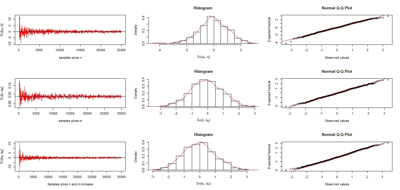
Figure 1. Plots when samples sizes increase, histograms and normal Q-Q plots of $\mathcal{D}_{T,\alpha}(p_{n},q)$, $\mathcal{D}_{T,\alpha}(p,q_{m})$, and $\mathcal{D}_{T,\alpha}(p_{n},q_{m})$ ($\alpha=0.99$) versus $\mathcal{N}(0,1)$.

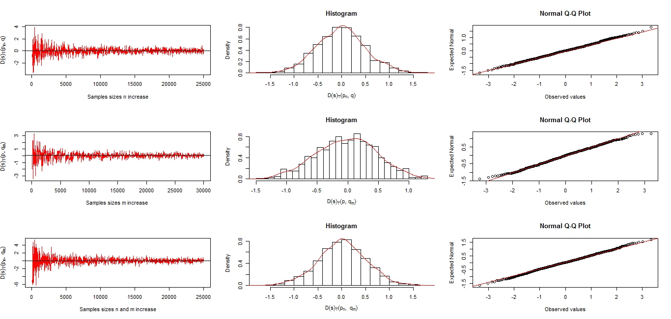
Figure 2. Plots when samples sizes increase, histograms and normal Q-Q plots of $\mathcal{D}_{T,\alpha}^{(s)}(p_{n},q)$, $\mathcal{D}_{T,\alpha}^{(s)}(p,q_{m})$, and $\mathcal{D}_{T,\alpha}^{(s)}(p_{n},q_{m})$ ($\alpha=0.99$) versus $\mathcal{N}(0,1)$.

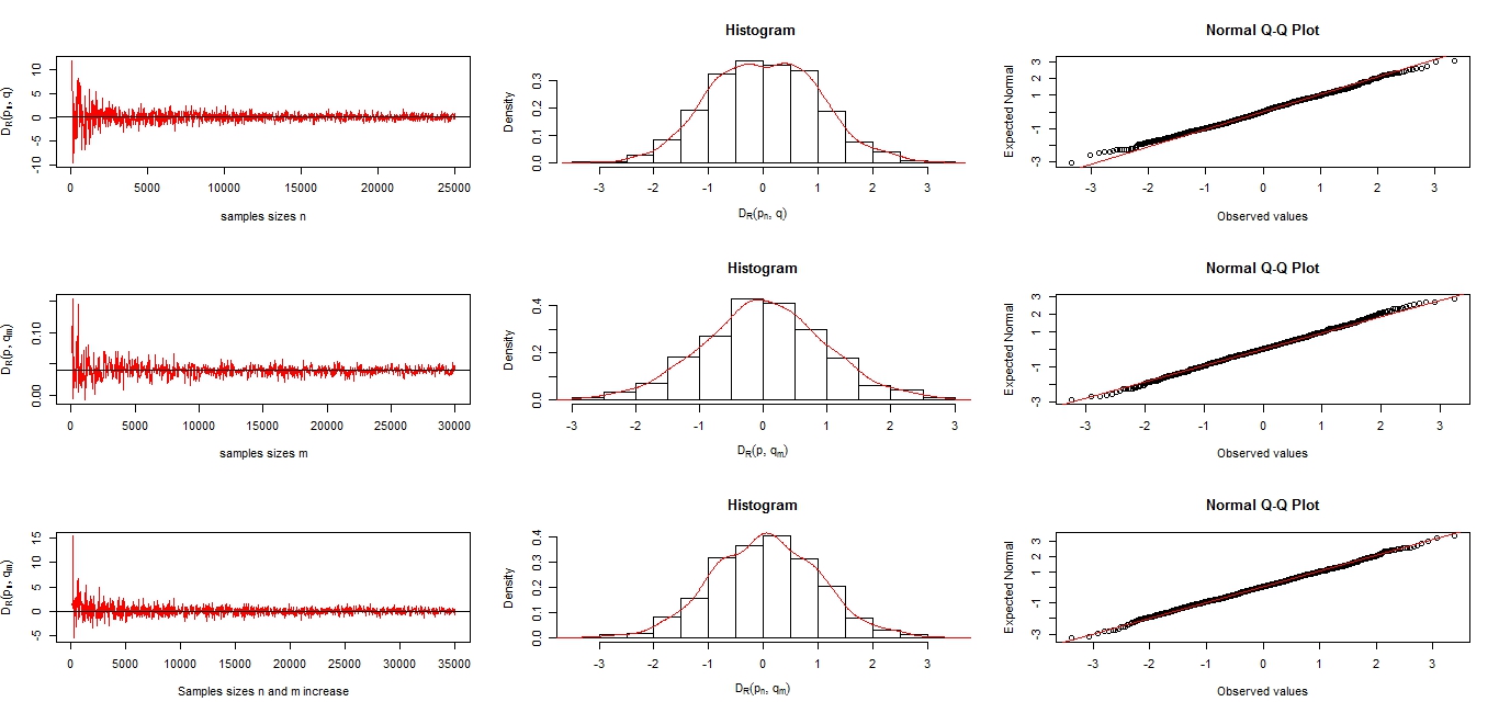
Figure 3. Plots when samples sizes increase, histograms and normal Q-Q plots of $\mathcal{D}_{R,\alpha}(p_{n},q)$, $\mathcal{D}_{R,\alpha}(p,q_{m})$, and $\mathcal{D}_{R,\alpha}(p_{n},q_{m})$ ($\alpha=0.99$) versus $\mathcal{N}(0,1)$.

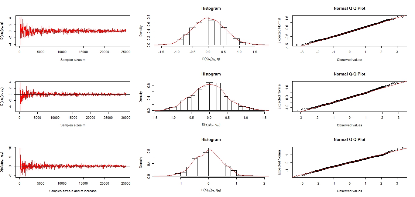
Figure 4. Plots when samples sizes increase, histograms and normal Q-Q plots of $\mathcal{D}_{R,\alpha}^{(s)}(p_{n},q)$, $\mathcal{D}_{R,\alpha}^{(s)}(p,q_{m})$, and $\mathcal{D}_{R,\alpha}^{(s)}(p_{n},q_{m})$ ($\alpha=0.99$) versus $\mathcal{N}(0,1)$

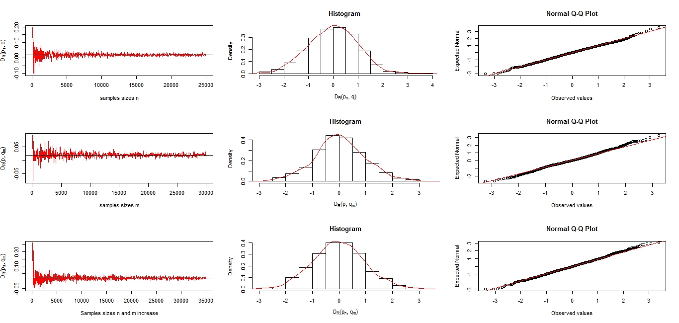
Figure 5. Plots when samples sizes increase, histogram and normal Q-Q plots of $\mathcal{D}_{R,\alpha}(p_{n},q)$, $\mathcal{D}_{R,\alpha}(p,q_{m})$, and $\mathcal{D}_{R,\alpha}(p_{n},q_{m})$ ($\alpha=0.5$) versus $\mathcal{N}(0,1)$.

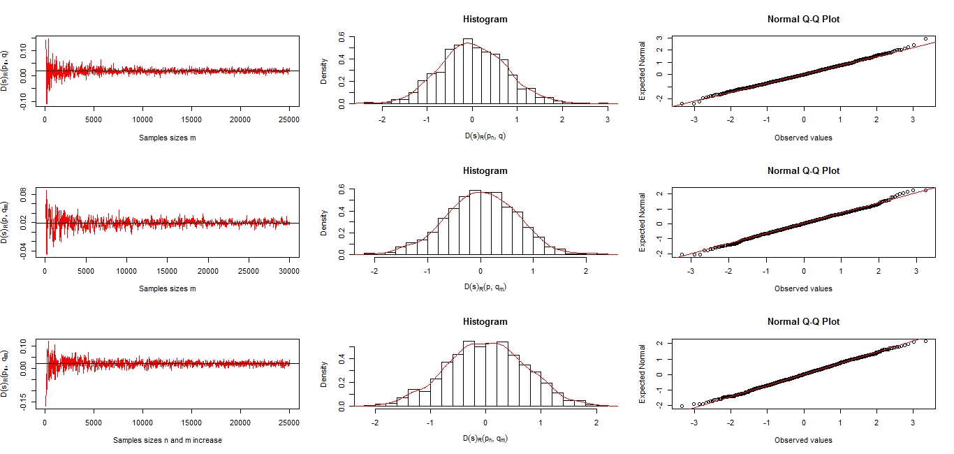
Figure 6. Plots when samples sizes increase, histograms and normal Q-Q plots of $\mathcal{D}_{R,\alpha}^{(s)}(p_{n},q)$, $\mathcal{D}_{R,\alpha}^{(s)}(p,q_{m})$, and $\mathcal{D}_{R,\alpha}^{(s)}(p_{n},q_{m})$ ($\alpha=0.5$) versus $\mathcal{N}(0,1)$.

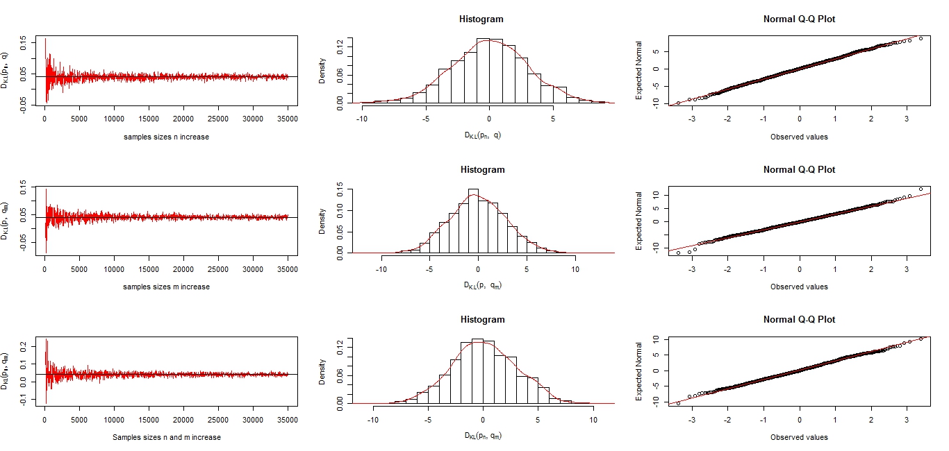
Figure 7. Plots when samples sizes increase, histograms and normal Q-Q plots of $\mathcal{D}_{KL}(p_{n},q)$, $\mathcal{D}_{KL}(p,q_{m})$, and $\mathcal{D}_{KL}(p_{n},q_{m})$ versus $\mathcal{N}(0,1)$.

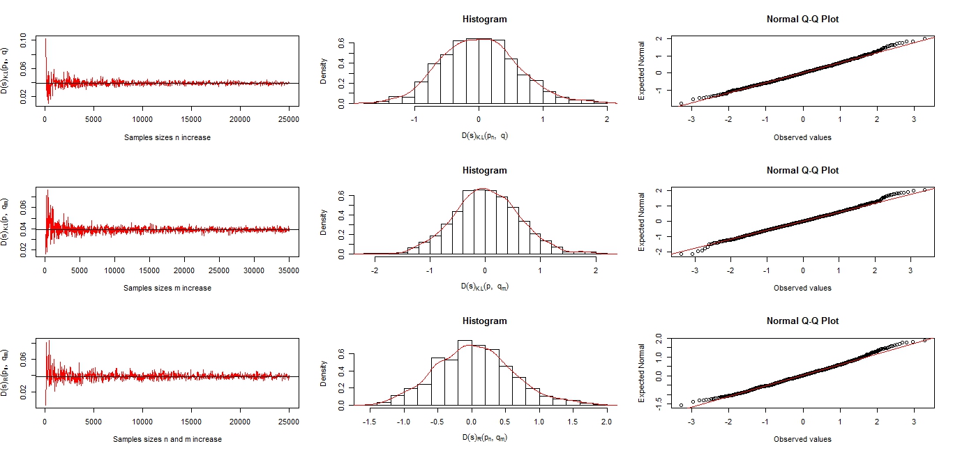
Figure 8. Plots when samples sizes increase, histograms and normal Q-Q plots of $\mathcal{D}_{KL}^{(s)}(p_{n},q)$, $\mathcal{D}_{KL}^{(s)}(p,q_{m})$, and $\mathcal{D}_{KL}^{(s)}(p_{n},q_{m})$ versus $\mathcal{N}(0,1)$.

7. Conclusion

This paper joins a growing body of literature on estimating divergence measures in the discrete case and on finite sets. We adopted the plug-in method and we derived almost sure rates of convergence and asymptotic normality of the most common divergence measures in one sample, two samples as well as symetrical form of divergence measures, all this, by means of the functional $\phi-$divergence measure.

References

• Lo et al. (2016) Lo, G.S.(2016). Weak Convergence (IA). Sequences of random vectors. SPAS Books Series. Saint-Louis, Senegal - Calgary, Canada. Doi : 10.16929/sbs/2016.0001. Arxiv : 1610.05415. ISBN : 978-2-9559183- 1-9
• Bâ et al. (2018) A.D. Bâ, Lo G.S and D. Bâ (2018). Divergence Measures Estimation and Its Asymptotic Normality Theory Using Wavelets Empirical Processes I. Journal of Statistical Theory and Applications. Vol. 17, Issue 1, p.158-171. https://doi.org/10.2991/jsta.2018.17.1.12
• Dhakher et al. (2016) Dhaker H., Ngom P., Deme E. and Mendy Pierre (2016). Kernel-Type Estimators of Divergence Measures and Its Strong Uniform Consistency. American Journal of Theoretical and Applied Statistics. Vol. 5 (1), pp. 13-22. doi: 10.11648/j.ajtas.20160501.13
• Topsoe (2000) Topsoe, F. (2000), Some inequalities for information divergence and related measures of discrimination, IEEE Transactions on Informations Theory, vol.46, pp.1602-1609.
• Evren (2012) Evren, A. (2012). Some Applications of Kullback-Leibler and Jeffreys’ Divergences in Multinomial Populations. Journal of Selcuk University natural and Applied Science,Vol.1(4), pp 48-58.
• Cichocki and Amari (2010) Cichocki, A. and Amari, S.(2010). Families of Alpha-Beta-and Gamma-Divergences: Flexible and Robust Measures of Similarities. Entropy, Vol.12(6), pp 1532-1568.
• Moreno et al. (2004) Moreno, P.J., Ho, P.P., and Vasconcelos, N.(2004). A Kullback-Leibler divergence based kernel for SVM classification in multimedia applications. Proc Adv Neural Inf Syst, vol.16, pp 1385-1392.
• Hall (1987) Hall,P. (1987). On Kullback-Leibler loss and density estimation. The Annals of Statistics, Vol.15(4), pp.1491-1519.
• Bhattacharya (1967) Bhattacharya, P.K.(1967). Efficient estimation of a shift parameter from grouped data, The Annals of Mathematical Statistics, vol.38(6), pp.1770-1787.
• Liu and Shum (2003) Liu, C., and Shum, H.Y. (2003), Kullback-Leibler boosting. IEEE Conference on Computer Vision and Pattern Recognition (CVPR), pp.587-594.
• Kullback and Leibler (1951) Kullback, S. and Leibler, R.(1951). On information and sufficiency. The Annals of Mathematical Statistics Vol.22,(1), pp 79-86.
• Cardoso (1997) Cardoso, J.(1997). Infomax and maximum likelihood for blind source separation. IEEE Signal Processing Letters., Vol.4, pp.112-114.
• Ojala et al. (1996) Ojala, T., Pietik ainen, M., and Harwood, D. (1996). A comparative study of texture measures with classification based on featured distributions. Pattern Recognition. Vol.29(1), pp. 51-59.
• Hastie and Tibshirani (1998) Hastie, T. and Tibshirani, R. (1998). Classification by pairwise coupling. The Annals of Mathematical Statistics. Vol.26, pp.451-471.
• Fukunaga and Hayes (1989) Fukunaga, K. and Hayes, R. (1989). The reduced Parzen classifier. IEEE Trans. Pattern Anal. Mach. Intell., Vol.11(4), pp.423-425.
• MacKay (2003) MacKay D.(2003). Information Theory, Inference, and Learning Algorithms. Journal of Experimental Psychology Cambridge University Press: Cambridge, UK
• Singh and Poczos (2014) Singh S. and Poczos, B. (2014). Generalized Exponential Concentration Inequality for Rényi Divergence Estimation. Journal of Machine Learning Research.Vol.6. Carnegie Mellon University.
• Krishnamurthy et al. (2014) Akshay K., Kirthevasan K., Poczos B., and Wasserman, L.(2014). Nonparametric Estimation of Rényi Divergence and Friends. Journal of Machine Learning Research Workshop and conference Proceedings, 32. Vol.3, pp. 2.
• Moon and Hero (2014) Moon, K.R. and Hero, III. A.O. , (2014). Ensemble estimation of multivariate $f$-divergence. in IEEE Internatonal Symposium on Information Theory, pp. 356-360.
• Lo et al. (2016) Lo, G.S.(2016). Weak Convergence (IA). Sequences of random vectors. SPAS Books Series. Saint-Louis, Senegal - Calgary, Canada. Doi : 10.16929/sbs/2016.0001. Arxiv : 1610.05415. ISBN : 978-2-9559183- 1-9
• Poczos and Jeff (2011) Poczos, B. and Jeff, S.(2011). On the estimation of $\alpha-$Divergences. In International Conference on Artificial Intelligence and Statistics, pp 609-617.
• Liu et al. (2012) Liu, H., Lafferty, J., and Wasserman, L.(2012). Exponential concentration inequality for mutual information estimation . In Neural Information Processing Systems (NIPS).
• Nguyen et al. (2010) Nguyen, X., Wainwright, M. J., and Jordan, M.I.(2010), Estimating divergence functionals and the likelihood ratio by convex risk minimization, IEEE Transactions on Information Theory, vol.56(11), pp.5847-5861.
• Valiron (1966) Valiron, G. (1966). Théorie des fonctions. Masson, Paris Milan Melbourne.
• Sricharan et al. (2012) Sricharan, K., Wei, D., and Hero, A. O. Ensemble estimators for multivariate entropy estimation. arXiv:1203.5829, 2012.