Sergio Bravo Medina
s.bravo58@uniandes.edu.co
Departamento de Física,
Universidad de los Andes, Cra.1E
No.18A-10, Bogotá, Colombia
Davide Batic
davide.batic@ku.ac.ae
Department of Mathematics,
Khalifa University of Science and Technology, Main Campus
Abu Dhabi, United Arab Emirates
Marek Nowakowski
mnowakos@uniandes.edu.co
Departamento de Física,
Universidad de los Andes, Cra.1E
No.18A-10, Bogotá, Colombia
Abstract
Cosmologies based on General Relativity encompassing an anti-symmetric
connection (torsion) can display nice desirable features as the absence of the
initial singularity and the possibility of inflation in the
early stage of the universe. After briefly reviewing the standard approach to
the cosmology with torsion, we generalize it to demonstrate
that several theories of torsion gravity are possible using
different choices of the diffeomorphic invariants in the Lagrangians.
As a result, distinct cosmologies emerge. In all of them it is possible that the universe
avoids the initial singularity and passes through an initial accelerated expansion.
Differences between these theories are highlighted.
Our understanding of the universe has undergone a revolution in the last decades. This is
mainly due to important observational discoveries like
the current accelerated stage of the expansion Peebles , precise
measurements of the Cosmic Background Radiation Penzias and other crucial
cosmological parameters Planck .
Yet a few cosmological puzzles are
still escaping a full explanation. Among them is the problem of the
initial singularity (best revealed by the Kretschman invariant
which tends to for the scale factor going to zero, )
and the nature and mechanism of early inflation which, in turn, seems to be a necessary ingredient of the early
cosmology to explain, for instance, the homogeneity and isotropy of the universe. Whereas it is certain
that we have several candidates for the inflationary scenario as well as for the
avoidance of the initial singularity, none of these theories seems to be fully accepted as
observational data, which could discriminate between these theories, are lacking and might continue to be missing for some time.
It is therefore of interest to explore different scenarios which provide us with
a solution. In choosing one of them a helpful guiding principle
might be the unifying wisdom of Occam’s razor: we consider a theory more
powerful and elegant the more phenomena it is capable to explain by
invoking a minimal number of new assumption and ingredients. A theory
like Einstein–Cartan could be the harbinger of such a unifying scheme.
It is a logical extension of Einstein’s General Relativity based on a new
connection which allows the former to have a symmetric (the standard Christoffel part) and
a new anti-symmetric part called contortion. As such the roots of this particular extension are
purely geometrical modifying, e.g., the geometrical part (say, the Einstein tensor as an example)
of the Einstein equations (this would be then unlike extensions which invoke new fields apart from the metric).
It is a physically consistent theory (this would be unlike some
theories with non-symmetric metric which do have deficiencies) which so far, is neither confirmed nor falsified. Indeed, it is fully unconstrained as
no data exist which could tell us something about its validity. Its appeal lies in the cosmological aspects or, to be more exact,
in the aspects which have to do with early cosmology.
It has been known for some time that the Einstein–Cartan cosmology leads to a singularity
free universe which at the same time can undergo an inflationary early expansion
thanks to the introduction of an anti-symmetric connection. The standard particular
Einstein–Cartan theory which has these desirable features is based on two pillars.
The first one is the Lagrangian chosen to be
where is the full Ricci scalar
obtained by using the connection , where is
the Christoffel connection and the anti-symmetric part called contortion.
The second basic ingredient is the choice of the physical source of the modified Einstein equations.
The Euler-Lagrange equations following from are not of the Einstein form
which coined on the general relativistic result would be ‘Einstein tensor being proportional to the source’.
Insisting on this form one adds a term on both sides of the equation which promotes
the left-hand-side to become the Einstein tensor (using again the full connection) whereas the right-hand-side
being the sum of the metric energy-momentum tensor and the newly added term is identified as the physical source
called customarily the canonical energy-momentum tensor. Both assumptions, the choice of the Lagrangian and the identification
of the canonical energy-momentum tensor as the physical source, are not stringent and, in view of the desirable features
of the Einstein–Cartan cosmology, it appears worthwhile to probe into other combinations and possibilities.
In a general setup of the Einstein–Cartan gravity there exist, apart from , several independent
diffeomorphic invariants which, in linear combination, can yield different suitable Lagrangians.
One can also identify the metric energy-momentum tensor inclusive new spin contributions as the physical source without running into
contradictions. Taken all together, new Einstein–Cartan cosmologies emerge which we will study in this paper.
We will demonstrate how, subject to the choice of parameters, they solve the initial singularity problem and can
display an initial accelerated stage of expansion. Three solutions of the former are logically possible: (i) the universe
is in a sense ‘eternal’ as it contracts to a minimum non-zero length (which we identify as the Big-Bang) from which it
expands Bounce , (ii) the universe is born spontaneously, but at a non-zero value of the scale factor and (iii)
the scale factor approaches its zero value only asymptotically at . We will probe into the questions
which one of these possibilities is realized in the Einstein–Cartan cosmologies.
Usually, the avoidance of the initial singularity is attributed to quantum effects (or a quantum gravity theory).
A question then arises what could be the input of quantum mechanics, if at all, in Einstein–Cartan theory. By inspecting the choice
of the source of the torsion part, this query can be answered. The aforementioned source is taken to be
where is the four-velocity and the tensor can be either
connected to the spin identifying it as one of the generators of the Poincaré–Lie algebra or as a classical angular momentum tensor
referring to extended bodies, see for details P1 ; P2 . In the early universe it appears more appropriate to refer
to spin rather than angular momenta.
In such a case is connected to the spin four vector by .
Here, the spin vector itself is usually associated with the expectation value of the spin operators
being proportional to the Planck constant . Hence, we could say that the source of the
torsion is of quantum mechanical origin. Indeed, the source could be a sum of two terms: one which can be traced back to the
spin and is phenomenologically taken as above and a classical angular momentum contribution which we will not consider here.
The spin tensor and the four-velocity are determined by the Mathisson–Papapetrou–Dixon (MPD) equations Mathisson ; Papapetrou ; Dixon
which depend also on the metric. Therefore, in principle, the modified Einstein equations and the MPD equations are coupled.
By using an averaging of the spin we can reach at a simpler system as we will explain in the main text.
There exist many reviews and books which expose the Einstein–Cartan gravity in detail Hehl ; Trautmann ; TrautmanNature ; Hammond ; PoplawskiInflation ; Odinstov ; ArcosPereira ; Boehmer ; Barrow . Here we take the occasion to review
the main aspects of the Einstein–Cartan cosmology to be able to make the comparison with the extension of these theories
made possible by starting with more general Lagrangians.
The paper is organized as follows. To make it complete we briefly review in the next section the conventions and
identities which enter the Einstein–Cartan theory, in general, and its cosmology, in particular. Section three
is devoted to the equations of motion derived from the Lagrangian . We present them in two different
forms, first in the standard way and secondly in a novel way after splitting off a total divergence.
We dwell upon this point because of a subtlety which follows and which is the identification of the
physical source. The original Euler-Lagrange equations are not of the usual Einstein form as mentioned already above.
These equations
have the metric energy-momentum as the physical source. Only after algebraic manipulation it is
possible to arrive at the Einstein form and choose the so-called canonical energy-momentum tensor as a physical source.
In the next section we discuss in detail the standard cosmology which emerges from the choice .
We identify the term in the canonical energy-momentum tensor which is responsible for the nice features of this cosmological model. Next we turn to alternative Lagrangians and their cosmological implications.
We present a simple, and a more general model and compare them with the standard one discussed in the preceding section.
As we will show in both models, it is possible to maintain the avoidance of the initial singularity and
have an accelerated initial condition on the expansion. All results depend on an averaging or the spin tensor.
Roughly, we assume that spin quantities entering our expression average to zero if we have to do with non-contracted open indices.
In section six we discuss briefly an alternative approach to this averaging for all models presented before.
In the final section we summarize our conclusions.
II Conventions and Identities
II.1 Conventions
Throughout the text we use the metric signature .
When torsion is introduced into spacetime, the standard identities and symmetries can be lost and makes sense to mention these differences explicitly before embarking
on the equations of motion and cosmology.
We derive our results following the notation and conventions introduced in Hehl .
We shall start with the definition of torsion as the antisymmetric part of the connection and thus a proper tensor
(1)
Apart from this definition demanding metricity with respect to the new covariant derivative, i.e. , the Einstein–Cartan (EC) connection is obtained
(see Appendix A for details)
(2)
where is the standard Christoffel connection
(3)
and is the contortion tensor, related to torsion by
(4)
(5)
For the sake of convention we shall use terms with an over-circle, e.g. ,
to refer to objects defined with respect to the Christoffel connection. For the Riemann tensor and the covariant derivative we use the same convention as in Hehl .
The covariant derivative of a mixed tensor is defined as
(6)
The Riemann tensor is given by 111D’Inverno Inverno has a different convention for the Riemann tensor and the covariant derivative, since one can always
think of a different order of the indices on this tensor, or even the order in the commutation relation MTW .
(7)
The signature of the metric is chosen to be . This sets our conventions.
II.2 General Results and Identities
Of interest are also general identities independent of the the equations of motion. This includes splitting the tensors into
the standard component defined over the
Christoffel connection plus a part with torsion (or contortion), Bianchi identities and other new identities.
For instance, by using the EC connection as defined in equation (2) we can write the Riemann tensor as
222In order to establish antisymmetry only on certain indices we use the
(8)
We may contract the Riemann tensor above to obtain the Ricci tensor.
On this convention the Ricci tensor is obtained through the contraction suggested in Hehl , i.e. . This yields
(9)
There is only one non-trivial contraction possible when going from the Riemann to the Ricci tensor in Einstein–Cartan theory, which can be seen from equations (7) and (8). Namely we see
(10)
Note that in the case of torsion the Ricci tensor is non-symmetric, unlike which is an essential part of the Einstein field equations in General Relativity.
We may write its antisymmetric part in the following way
(11)
where we have defined the modified torsion tensor
(12)
as well as the star derivative333Note that the star derivative has the following property when acting upon a vector
.
(13)
We can contract the full Ricci tensor to obtain the Ricci scalar in terms of torsion or contortion
It can be easily shown that with . Then the Ricci scalar in terms of torsion and contortion yields
(15)
(16)
All terms in (16) are invariants and as such they are candidates for a Lagrangian built up by a linear
superposition of these terms, the Ricci scalar being only one possibility. We will examine such theories and apply them
to cosmology.
Apart from the relations found above, it is often useful to have some analogue to the standard Bianchi identities and
conservation laws in Einstein–Cartan Theory Schouten ; PoplawskiFields . Since we are indeed looking for identities similar to the Bianchi identities, these must give the
standard Bianchi identities when the torsion is put to zero.
To derive them we start with the commutator of the covariant derivative
acting on an arbitrary vector. Given the connection in Einstein–Cartan
we obtain
(17)
which means that we are entitled to write
(18)
We also obtain the following antisymmetric condition on the covariant derivatives
(19)
This can be re-organized using the commutator on equation (17) as follows
(20)
Finally antisymmetrizing in the three indices we get from equation (18)
By equating these equivalent expressions we see that the following identity holds
Comparing in the next step the and coefficients we obtain the equivalent to the first Bianchi identity
(23)
and the second Bianchi identity which involves only torsion
(24)
The first Bianchi identity may be contracted to yield
(25)
(26)
Defining a new Einstein tensor over the full connection
(27)
we can appreciate how the last result helps us to obtain the covariant divergence of the Einstein tensor
(28)
So far, our results were independent of the equation of motion. We can apply them also
directly to the equations of motion.
There will be two sources in the theory, one for the modified Einstein equations which for now
we write as and for the torsion which we call .
By using the derivative we can recast the result (28) as
(29)
Some straightforward manipulation gives
(30)
Anticipating part of the results derived explicitly later i.e., using equation (57)
which yields in terms of torsion we can write
(31)
In case our equation of motion is of the form this equation is the new ’conservation law’.
For completeness we mention that in HehlPart2 this ‘conservation law’ is written defining the following derivative
(32)
valid for only covariant indices in the form
(33)
Finally, we are aiming at an identity relating the antisymmetric part of to the source of the torsion.
The expanded second Bianchi identity is
(34)
On the other hand, one can also show
(35)
Combining the two equations above appropriately, we obtain
(36)
which still lacks an explicit physical interpretation. However, we are able to derive an identity
which we will need in the next section
(37)
III Lagrangian and Equations of Motion
In Einstein–Cartan Theory it is generally assumed that the Lagrangian be taken proportional to the Ricci scalar in a
space-time with torsion. From its
variation the equations of motion are obtained, as in any other theory in which a Lagrangian formalism may be applied Variations-GR .
However, there seems to be
a preferred approach to these equations of motion, which lead - quite nicely - to
an equivalent expression to the Einstein Field Equations (EFE) defined over the full
connection. We will show in
this section that this is not the only approach in which one can obtain the field equations and, moreover,
the alternative way of approaching them leads to equations of motion which are in principle different
but can formally be transformed into the
standard result. Given these equivalent expressions, the question arises what is the physical interpretation of the energy–momentum tensor
in each one of these approaches.
III.1 Standard Approach
What we shall call the standard approach to the variational principle is discussed in
Hehl and some details can be found in HehlPart1 ; HehlPart2 ; HehlPRD .
We
will see that the key to this approach is to work directly with the quantities of the Riemann–Cartan geometry without having to go back to the usual General Relativity geometrical
quantities defined over the Christoffel symbol.
We start from a gravitational Lagrangian given by , so that the full action, including a
matter Lagrangian, is
(38)
Varying the gravitational portion of the action with respect to the inverse metric yields
(39)
where we have . Now, can be obtained from the contracted Riemann tensor
which, using the definition of the covariant derivative given above, yields
(40)
Contracting the first term with reveals an explicit total divergence
(41)
This divergence is neglected and taken out
(see the Appendix of Hehl ) so that the relevant parts of the term are now
(42)
where we have used the modified torsion as defined earlier. For the variation of the connection with respect to the metric we use Ortin
(43)
and thus, we obtain
(44)
We put this term into the integral after which, in order to integrate by parts, it is worth noting that for each of these three terms we get expressions of the form
(45)
Integrating by parts for the first term on the right hand side gives
(46)
where the last term on the right is a full divergence and can be neglected. Finally, using the definition of the star derivative and adding up the three terms we have hence
(47)
We note that
(48)
We recall that the new Einstein tensor is in analogy to its GR equivalent. The symmetrization
of this new Einstein tensor (EC tensor)
is due to the fact that we are contracting it with a variation of the metric, making any antisymmetric part of the tensor arbitrary and thus not relevant
Variations . The remaining terms of the variation
(49)
should also be symmetrized. After this we arrive at
(50)
where we have left only the symmetric terms. Due to our previous result (36) ,
the variation with respect to the metric is simply HehlPRD
(51)
On the other hand, for the variation with respect to contortion we have
(52)
where we have used the results from the variation with respect to the metric shown in equation (42). Furthermore, we find
(53)
With this result we are led to
(54)
Concentrating on the matter sector of the Lagrangian , we define
the metric energy–momentum tensor and the source as
(55)
With all the results we can set up the field equations as
(56)
(57)
Note that the variation with respect to contortion is just an algebraic equation for torsion in terms of its source which can be also
cast into a form using the modified torsion
(58)
Referring to as the non-symmetric total energy-momentum tensor or
as the canonical energy-momentum tensor defined by
(59)
leads us to equations of motion of the Einstein form
(60)
From the algebraic torsion equation it follows that
(61)
(62)
It is, of course, mandatory to be able to express the torsion or contortion in terms of the source.
Splitting the symmetric part of the modified Einstein tensor into its torsionless part plus terms related to torsion , i.e. , using equation (36) for the anti-symmetric part expressed through the star covariant derivative
and finally expressing all torsion terms through the source we arrive at an equation of the form
which reads explicitly
(63)
This means that the dynamical equation of motion for the metric can be brought into the form
(64)
Here, will include the torsion source terms
(65)
All equivalent reformulations have only a physical meaning after we specifically state what is the source of the dynamical equation.
Indeed, looking at Eqs. (59), (60) and (63) it is clear that the term proportional to
cancels from the Einstein tensor and the canonical energy-momentum tensor unless we identify/fix the canonical energy-momentum tensor as
the physical source or, equivalently we insist that the equations of motion must have the Einstein form .
In such a case the equations of motion are of the form with all torsion terms
expressed through it source. The metric energy-momentum tensor drops out from the picture here.
Though consistent and
logically possible, this is not stringent.
III.2 Alternative Variational Approach
To demonstrate how the equations of motion come out naturally in a non-Einstein form let us apply an alternative method to the
variational principle splitting, right from the beginning, total divergences.
The starting point of an alternative approach to the variation of the Lagrangian is precisely the same, namely we shall take the action
(66)
where is the matter Lagrangian and (we have taken ).
We write the Ricci scalar in Riemann–Cartan theory explicitly in terms of its torsionless portion and parts related to the torsion so that
in the process a total divergence as in equation (16) appears which we discard. We define the divergence-less part of the Ricci scalar, , as
(67)
which is just a divergence-less version of equation (15).
We interpret it as an equivalent Lagrangian whose action we call
Next we vary this action with respect to the metric, which simply yields
(71)
along with the standard result,
(72)
Examining the last term on the l.h.s. we note that it is a full divergence as in standard GR and will not contribute to the action. Taking into account that
(73)
we obtain then the following field equations, where is the metric energy–momentum tensor we have already defined,
(74)
We can abbreviate the term on the right hand side involving only contortion tensors as the symmetric tensor (see below) in which case
our equations of motion have the form .
Given that the algebraic equation for torsion is the same as we obtained in the standard approach, we can make use of the results given in equations (61) and (62) to write
(75)
These results mean that in terms of the tensor our equations of motion are of the form
(76)
Note that in this derivation no terms involving
are present and yet the equation above is formally equivalent to the one obtained in HehlPRD ; HehlPart1 ; HehlPart2 .
In order to account for this
equivalence we point out that adding on both sides a term proportional i.e.,
we obtain the Einstein form
With the following tensor
(77)
there is indeed a formal equivalence between the two approaches, namely,
(78)
where, to get the equation on the right we need to add the term on both sides of the equation. However, it is also clear that the equation of motion comes out in the form and only the insistence on the
analogous Einstein form leads to . Of course, formally these forms are equivalent. The two approaches will differ once we identify the physical source as or
. This will be outlined in the next sub-section.
III.3 Identification of the Energy–Momentum Tensor
If the matter Lagrangian is uniquely given by choosing it to be the Dirac or Klein–Gordon Lagrangian
then, the answer to the question of which of the aforementioned approaches one should use is easily answerable.
The matter Lagrangian fixes the metric energy-momentum tensor and therefore, the terms proportional to cancel on both sides
of the equation of motion given in the form leaving us with . One could argue that alone
for this reason the form with chosen to be the physical source is always preferable, over with
the physical source, even if we handle a phenomenological energy-momentum tensor. However, even if we follow this path, there is still place
for new contributions to the phenomenological energy-momentum tensor coming from the source of the torsion.
Especially, when turning to cosmology one is faced with the question of the choice of the energy-momentum tensor,
given that in torsionless standard cosmology one usually takes a perfect fluid
energy–momentum tensor.
We follow the approach taken by some authors of including spin into the energy–momentum
tensor, motivated by the fact that torsion is a manifestation of spin SabbataBook .
Here, we are faced with two options which we will study independently, (i) we could take the construction given in HehlPRD ; PoplawskiInflation ; Variations
following the full Einstein form as in equation (60) and work with the so called canonical energy–momentum tensor .
Alternatively, (ii) we could take the construction obtained from varying the Lagrangian after splitting off
total divergences, namely equation (76), and identify as the physical source admitting room for contributions with spin.
We will examine different choices of the energy–momentum tensor in
these two approaches below.
Our starting point is to determine the
canonical energy–momentum tensor which we assume to be of the form Kopczynski1 ; Kopczynski2
(79)
where is the pressure of the fluid, is the four-velocity and is the enthalpy density.
An expression for the enthalpy density can be obtained from the identity (31)
(80)
and the requirement (coined upon a similar result in the standard hydrodynamical energy-momentum tensor)
(81)
As a result, choosing the source of torsion as spin tensor multiplied by velocity
which by anti-symmetry of the spin tensor implies .
By virtue of (80) we find an interesting relation, namely
(84)
in which last term is zero given that . The simplified version reads now
(85)
Again, the last two terms with contortion and the spin tensor can be shown to yield zero by using equation (62) along with the Frenkel conditions.
Invoking as before , we find that
(86)
Finally, contracting equation (85) with , we obtain
(87)
which fixes the canonical energy–momentum tensor
(88)
By identifying the canonical energy–momentum tensor as the physical source, the metric energy-momentum tensor (see equation (59)) has dropped out from the picture, but it is useful
to define formally a similar expression
(89)
where we have kept the terms symmetric in . For the sake of later references to this quantity, we will refer to the term proportional to
as the Weyssenhoff term and to the term proportional to simply as the -term.
In (98) we can replace the covariant derivative with respect to the Christoffel connection by the full
covariant derivative with respect to the full connection.
A few comments on the spin tensor are in order. First note that is related to the spin vector
by . Interpreting the spin vector as an expectation
value of quantum mechanical spin operators, will be proportional to reminiscent of its quantum mechanical origin.
Relating the source of the torsion to quantum mechanics might help us to understand why the Einstein–Cartan cosmologies can avoid the
initial singularity.
Secondly, the microscopical quantities within this theory will be fluctuating, thus it is common to take average values of these quantities. If indeed spin orientation
is random, then the average of the spin will vanish, but not the terms that are quadratic in spin Hehl . Given this non-vanishing quantity, the average of the square of the
spin is taken to be444A different notation in PoplawskiInflation ; PoplawskiSingular ; PoplawskiBH .
(90)
where we follow the notation in HehlPRD as far as the quantities with spin are concerned.
Taking and respecting the Frenkel conditions
we can write
(91)
where the -terms have contributed to the
terms in the square brackets.
It is also worth noting that in cosmology (which we consider in the subsequent section)
the comoving reference frame together with the Frenkel conditions yields a ‘new’ condition, i.e. ECWormhole . Adding to the components of
(see equation (77)) we arrive at
(92)
The contributions of that yield non-zero expressions in the co-moving frame are
(93)
(94)
(95)
The term (93) cancels with the last term in (91). The modified energy–momentum tensor will finally be
(96)
The equations of motion here are of the form . Next, we turn our attention to the second possibility of identifying the metric energy–momentum tensor as the physical source.
As outlined above in sub-section B the variation of the Lagrangian with respect to the metric leads to the equation
of motion . There is no doubt that this is the correct result and only formally equivalent to .
If we view as the physical source, we can repeat some steps from above. i.e., we write as an ansatz
(97)
and impose as before. This gives us the equation . With the first choice being ,
the other possible terms denoted here by have to give zero when contracted with the four-velocity . Hence,
by virtue of the Frenkel condition we can have
.
We recognize in the second term the Weyssenhoff spin contribution mentioned before. But, in general, we can choose any combination of allowed contribution.
Motivated by the result found in ObukhovSpin ; Obukhov which claims that the spin contribution to the standard hydrodynamical
energy-momentum tensor is of the Weyssenhoff form, we opt here for
(98)
The equations of motion are of the form now .
IV A Note on the Connection between Torsion and Quantum Fields
We focus throughout this paper on geometric aspects of torsion applied to cosmology.
It is, however, certainly worthwhile to mention briefly the connection of
torsion to (fermionic) quantum fields. The first such a link can be found
by noticing that the source of torsion, which in the present paper we treated
in a more global manner, can be also found in the spin part of the angular
momentum tensor which arises in quantum field theory by the invariance of the
matter Lagrangian with respect to proper Lorentz boosts Bjorken .
For example, for the Dirac field we would have
where stands for the Dirac field Dirac1 ; Dirac2 .
Of course, by making this choice the full system to solve would consist of
Einstein equations with torsion and the Dirac equation coupled to gravity.
Secondly, in the coupled system torsion gives rise to the so-called
Hehl–Datta term Kibble ; Hehldatta which is a ‘bare’ four fermion
interaction term of two axial currents. This has led to new lines of research
Fansworth ; Weller ; Poplawsky2001 ; Poplawsky2011 ; Poplawsky2011b ; Boos2017 speculating on new propagating massive degrees of freedom,
new contributions to the matter-anti matter asymmetry and the cosmological
constant (or Dark energy in general) as well as the demonstration of
the possible formation of Cooper pairs due to the Hehl–Datta term.
Finally we point out the connection of torsion to the photon as discussed
e.g., in SabbataBook .
V Standard Einstein–Cartan Cosmology
In this section we investigate the consequences of the standard Einstein–Cartan cosmology based on the identification of the canonical energy–momentum tensor as the physical source Atazadeh ; Ritis .
As discussed above our equations are .
In order to study this cosmological model we must obtain the Friedmann equations from the field equations (64). Let us take the Friedman–Lemaître–Robertson–Walker metric in its flat version, i.e. , and in the sign convention as we have used before. This metric is given by the line element
(99)
with the scale factor Carroll .
The Friedmann equations are obtained from the time–time and space–space components of the field equations. Let us first write explicitly the field equations we will be working with, namely
(100)
We can now take the component of the field equations to obtain the
first Friedmann equation. Let us concentrate on the r.h.s. given the Frenkel and the rest frame conditions (recall that ), we note that the term with explicit spin tensor dependence is zero, i.e.
(101)
This makes it quite straightforward to derive the first Friedmann equation
(102)
where . This is one of the crucial forms of the Friedmann equations which avoid the singularity and leads to a bounce. It defines
a critical density when the right hand side of (102) becomes zero which implies that at a certain time
the Hubble parameter is also zero. This suggests that the Hubble parameter can have a local minimum, a sign
of a bouncing universe. Such forms appear in theories such as Loop Quantum Cosmology models LQCStatus , Generalized Uncertainty Principle approaches MinimalLength or quantum corrections in Newtonian Cosmology BBN1 .
For the second Friedman equation we take the space components of the field equations where again it is
worth noting that the last term (the Weyssenhoff term) on the right of the Einstein equations is zero because of the rest frame conditions.
The second Friedmann equation is simply
(103)
where we defined .
This Friedmann equation can be written using equation (102) in the following form
(104)
Equations (102) and (103) match the ones given in PoplawskiInflation with the choice . Combining both equations one can also find that
a conservation equation emerges
From this relation and by using an equation of state of the form , one obtains via integration
(107)
We will also have the following relation for the spin density of a fluid of fermions with no spin polarization
(108)
which means that we can relate spin density to energy density according to
(109)
where is a coefficient with dimension which depends on the value of . Using this proportionality in the continuity equation, we may solve for in terms of .
Let us start by taking equation (105) in the form
which, as long as (or rather ) gives the standard
General Relativity result
(112)
From this point on, we will choose . It is now easy to see that the proportionality of and is given by
(113)
where this proportionality is independent of given the relation found in equation (109). As we have stated before, the spin effects will be significant during high density
eras, that means that we will be interested in the radiation dominated era, and so, from here on, we will take . In this regime the first Friedmann
equation will be
(114)
Note that given the factor of the spin part on the r.h.s.
of the equation above, these terms are expected to
be dominant at high densities of matter.
We can integrate the above equation to yield
(115)
which according to PoplawskiSingular , gives a non-singular universe.
We confirm that indeed this is the case by choosing and thus which simplifies the above expression, more precisely
(116)
As already mentioned we have a critical density at which becomes zero. For it is given by
(117)
We also see a restriction upon the value of in the solution above, namely
(118)
by virtue of .
We note that by making the obvious choice we have and this also implies
(119)
The expression for given in equation (116) simplifies to
(120)
where . We plot this expression
for the two possible signs, which refer to an expanding universe ()
or a contracting universe (), and we note that the branches can be
taken as one solution given that they are differentiable at the place where they match (see Figure 1).
This represents the aforementioned bouncing universe.
Figure 1: Plot for the two signs of equation (120) which correspond to the contracting () and expanding () solutions where
the bounce at is indeed differentiable.
Within this theory the possibility of inflation has also been considered in Gasperini ; SpinInflation , and more recently in PoplawskiInflation .
We briefly outline the basics here.
One of the possible
inflation stages occurs when and , referred to as ‘super-inflation’ SuperInflation ; Lucchin . Since we have
(121)
taking the radiation case and the relation between and given above, we obtain that this is possible as long as
(122)
where we must also note that the second requirement comes from
(123)
which implies whenever
(124)
The bound is a strong requirement but still within the possibilities of the model. The transitional stage of this process will be determined by an exponential stage of inflation
which has been suggested by Guth InflationGuth . Here, it corresponds to the particular moment at which , or equivalently when the density is .
Thus, we have the following scenario
The model expressed above is the standard approach to Einstein–Cartan cosmology
Gasperini ; PoplawskiBounce . In the following we will explore how a different choice of the physical source may affect these results.
Indeed, it is almost mandatory to pin down the term which is responsible for the nice feature (especially the avoidance of the initial
singularity) of the theory. To this end we simply drop by hand all the -terms in (98).
Hence, we will work simply with
(125)
where we have already used one of the Frenkel conditions to write the source of torsion in terms of the spin tensor.
It is clear to see that this result is basically the perfect fluid part plus
an additional term due to Weyssenhoff (this term is symmetric as would be expected) Ziale ; Oliveira . Once we implement it into cosmology the result is the same as if we would have a perfect fluid identification. This is due to the
Frenkel conditions and the comoving frame condition.
Its effect upon the field equations gives an effective energy–momentum tensor of the form
(126)
where we have used the Frenkel conditions Frenkel , i.e. equations (83).
Now apart from this we have also assumed that the average over the contraction of two spin tensors is not negligible and actually takes the form we established before . Furthermore, we will follow Gasperini’s result and take
(127)
which is a result given implicitly in Gasperini 555For the interested reader we suggest checking equations (4) through (9) in Gasperini and noting that his result indeed suggests
the value for this average.. With these conditions the Friedmann equations are given by
(128)
Using both of these equations we can write
(129)
Under the assumption that we are dealing with fermions and that there is no polarization of spins in an ideal fluid Nurgaliev , we can use the relation between spin density and
particle number density obtained in equations (108) and (109). Now we can construct the continuity equation
(130)
which is obtained from the
Friedmann equations we found above. Equivalently, we can write it in the following form
(131)
The solution of the differential equation is
(132)
We can see that, while it is not exactly the standard GR case (see Appendix B), equation (132) shows that when the density goes to high
values , the scale parameter will approach zero as in GR. There is no restriction upon and thus we may
interpret that we are not avoiding the singular behaviour. In order to study this system further, we will make the change of variables
(133)
With these new variables the first Friedmann equation turns out to be
(134)
We replace this in the differential equation for and rewrite as
(135)
This equation can be solved analytically giving us
(136)
where is a constant given by the integration limit
(137)
We choose the sign that reproduces an expanding universe. With this in mind and looking at the plot of for this
expanding solution (Figure 3),
it is clear that grows arbitrarily as approaches negative values, which reinforces the idea of the density approaching an infinite value at early times.
Equation (136) is as far as we may go analytically, but we can get further insight confirming our conclusions so far by solving the equations numerically.
Figure 2: Plot of as given by equation (136) with both sign choices. Note that the dashed line corresponds to a contracting universe.
Figure 3: Plot of as the numerical solution of equation (135) with initial value .
With the help of MATHEMATICA we first obtain a numerical solution for the solution for that corresponds to an expanding universe,
which we have plotted in Figure 3.
The behaviour of in terms of is also obtained numerically by taking equation (134) and integrating
Figure 4: Plot of the numerical solution of from the positive sign of equation (138) for an initial value .
Note that for the expanding universe solution in this model, i.e. the one with , as one goes to the past () reaches
zero unavoidably, suggesting it does not avoid the initial singularity. In conclusion, it is the term proportional to which is responsible for the
nice features of the model. In the next section we will present models which do not include this term, yet display an absence of the singularity, and eventually also an accelerated behaviour
of the expansion in the early universe. To this end we will make use of different Lagrangians.
VI Alternative Lagrangians
Following our aim of studying alternative treatments of space time with torsion, an important observation is that the choice of the Lagrangian in ECT is not stringent to start with the identification ,
although it is perhaps aesthetic. Indeed in space-time with torsion we have the following independent diffeomorphic invariants
(139)
Therefore, a more general Lagrangian could be constructed out of a linear combination of these terms for an alternative approach to Einstein–Cartan Theory. Our final goal is to
examine the cosmology based on the following
Lagrangian
(140)
(141)
where the are dimensionless coefficients. Note also that we have explicitly neglected the total divergence term present in standard ECKS. The particular
choices of , and would account for the case
explored in the preceding section. Indeed, a linear combination of invariants is similar to the starting point of Teleparallel Theory
and particularly, the Teleparallel Equivalent of General Relativity (TEGR) in which
the effects attributed to curvature are now replaced by effects of torsion TeleparallelBook ; TEGR . This theory has been quite studied in recent years after the Hayashi construction Hayashi1979
of scalar fields behaving differently in TEGR which gives rise to alternative views of dark matter behaviour Otalora . We mention also the possibilities
of theories with the scalar constructed from torsion invariants FTTheories ; TomiTeleparallel which matches the behaviour of in GR.
Inspecting the form of equation (141) we see that a simpler version is also possible.
Before embarking on the general case, it is instructive to use first this simplified version of the above invariants using only contortion, namely
(142)
where it is relevant to note that this approach, while including essentially the same invariants, is a simplification of the more general case with a certain relation between the
coefficients. From these invariants we can construct the following Lagrangian with arbitrary coefficients and (this case corresponds to the
particular choice in equation (141) and taking and )
(143)
The Lagrangian is now with the action
(144)
where is the matter Lagrangian. We first vary the action with respect to the metric to obtain
the field equations which may be written as
(145)
The algebraic relation which emerges upon variation of the contortion
can be put in the following form
(146)
(147)
We recover the ECKS standard case when taking the proper values for the coefficients , namely . By taking the trace of the spin energy-momentum tensor in the
equation above we get
(148)
which means that we can write the torsion tensor in terms of its source as
(149)
and similarly, the contortion in terms of
(150)
The last equations show that we can solve the algebraic equation in terms of the source.
With this at hand we can write the full field equations coming from the variation with respect to the metric in terms of the spin energy-momentum tensor as
(151)
The Frenkel conditions (83) lead to a major simplification of these equations and one obtains
(152)
VI.1 Cosmology in the Alternative Lagrangian
The standard choice of General Relativity is taking the standard hydrodynamic perfect fluid energy–momentum tensor to which a spin-dependent Weyssenhoff
term is added.
We must note that this further term will, however,
not contribute to the cosmological equations because of the Frenkel conditions. For a perfect fluid with spin we have the following energy–momentum tensor
(153)
Setting this into the field equation and using both Frenkel and comoving frame conditions yields
(154)
As usual the Friedmann equations will be obtained by taking the diagonal components of the field equations. From the time–time components we get
(155)
while the space–space diagonal terms give
(156)
From the last equation it is clear that we cannot have an accelerated stage in this model.
Both Friedmann equations result in the continuity law of the form
(157)
Using the relation for the particular case of radiation given that we are interested in the early universe behaviour
we take and rewrite the continuity equation as
(158)
A quick examination of the Friedmann equations and the continuity equation suggests that a positive value for will just be a slight generalization upon
the solutions obtained at the end of section IV
with a singularity present at the beginning of the universe.
But, if we consider the case in which , we see that this choice will have an essential impact on the Friedmann equations. Moreover, it will indeed define
a particular maximum density given the form of the first Friedmann equation. We already mentioned that the possibility of the Hubble parameter becoming
zero at some time can eventually lead to a model of a bouncing universe. With a negative we would have ,
but the model exhibits a more complicated hierarchy of three different critical densities which prevent
the situation in which . To see that, we start by expressing the scale parameter through the density by integrating the continuity equation
(159)
leading to
(160)
As a result
can be rewritten in terms of as
(161)
To obtain in terms of would imply solving a fourth order equation which will not give any useful insight into the Friedman equations.
We will therefore not pursue this path to solve the Friedmann equations.
Instead, we will use the continuity equation of the form
(162)
Replacing therein, the first Friedman equation
(163)
it is possible to arrive at a relation between and from
(164)
The scale factor can be obtained either by integration of (162) and by replacing into (161). Before embarking on this programme it is mandatory to probe into critical densities of this model.
We recall that under the condition
the first Friedmann equation acquires a form reminiscent of bouncing cosmologies, i.e.
(165)
and obviously suggests a possible critical density. Given that we have
(166)
It is interesting to see the value of the scale factor corresponding to this
(167)
where the appearance of complex value of shows that this is not possible.
Indeed, the model has three different critical densities out of which one is the defined above.
For a negative the continuity equation reads
(168)
or equivalently,
(169)
where
(170)
The hierarchy of the three critical densities is
(171)
We see that only is physically allowed since the inequality must be satisfied to avoid complex values of the
Hubble parameter. When this happens, i.e., hits , the r.h.s. of the continuity equation vanishes, and this
suggests that either or or .
Indeed, and are not possible whereas would imply which leads also
to a contradiction.
Mathematically, we can have or . We will see that a physically viable
expanding universe must obey the first chain of inequalities thus making a bouncing universe impossible. This, however, does not exclude a scenario where the universe is born at a non-zero scale factor.
With this in mind we write the continuity equation (169) in a dimensional-less form by introducing the following variables
(172)
The continuity equation takes form
(173)
where the strongest bound on is . The physical solution will reveal a stronger bound, namely
(174)
The unphysical bound involving corresponds to . Next, we will make use of the first Friedmann equation in this approach
and rewrite it in the form
(175)
Replacing this in the continuity equation we obtain a differential equation for , namely,
(176)
where all three critical densities are manifest.
We have solved this equation numerically and plotted the results for a particular
initial value of in Figure 5.
Figure 5: Numerical solution of equation (176) with the negative sign and initial value . We have drawn the maximum allowed density as well.
The solution has an initial value slightly smaller than corresponding to . It is evident that does not exceed the critical value .
We will come to this point below.
In these plots we have also included the critical values mentioned earlier, where we note that is definitely a forbidden value, and we have that either
or , which evidently truncates the solutions obtained.
We may also take this solution for and use it in the first Friedmann equation.
We find a solution for given by
(177)
which we solve numerically. We plot these numerical solutions in Figures 7 and 7.
Figure 6: Plot of the numerical solution to equation (177) with initial value . We show both solutions, with the growing solution the one corresponding to the positive sign.
Figure 7: Plot of the numerical solution to equation (177) with initial value .
Alternatively, if we keep in mind that , we obtain using equation (173)
(178)
Computing from equation (178) and
changing time in terms of , it is possible to get an implicit expression for
which when integrated gives
(179)
Figure 8: Plot of the upper sign of equation (179) which corresponds to an expanding Universe and suggests the behaviour of in terms of . We have plotted the critical values and . Consistently we have to take the lower branch of the curve.
Figure 9: Same as Figure 9 with a different initial value .
Figure 10: Plot of the lower sign of equation (179) which corresponds to a
contracting Universe. In this case we also choose the lower branch.
Note that in the plot of equation (179) (see Figures 9 and 9, where the sign has been chosen for an expanding universe),
a non-invertible behaviour is evident from the point when it reaches
the first critical density . We also note that
the maximum density defined from the first Friedmann equation, given by , will indeed be a value beyond which will never go.
Mathematically, is possible, but can be excluded on physical grounds for an expanding universe. We have also plotted the solution for a contracting Universe in Figure 10.
VI.2 Cosmology in the Alternative Lagrangians
Let us go back and consider the Lagrangian in equation (140).
In order to obtain the equations of motion we vary the Lagrangian with respect to the metric tensor and
the
contortion tensor. The variation of with respect to
the inverse metric will yield the following field equations
(180)
where is the metric energy–momentum tensor defined in (55).
The variation of the Lagrangian with respect to contortion results in the following algebraic equation in terms of contortion and its source
We can now relate the source of torsion in the following way
(184)
Using (184) it is possible to write the torsion in terms of its source only. We have
(185)
where we have defined a tensor as
(186)
The contortion will be written in terms of as
(187)
This result implies that we can write the metric field equations in terms of the source .
Indeed, after some manipulations and by defining the following coefficients
we get
(188)
which, upon invoking the conditions for the source represented by (83) and performing an averaging over the spin terms,
can be considered satisfied. For instance, already the tensor takes a simpler form
(189)
Following Gasperini , expressions of the form , i.e., spin expression with an open index,
average to zero while averages to . The final result is
(190)
To proceed further we need to specify the energy-momentum tensor
which we take to be that of a perfect fluid plus a spin contribution of the Weyssenhoff form.
Hence, we get
(191)
The Friedmann equations in this case can be obtained formally as before. Therefore, we just quote the result
(192)
(193)
A small manipulation gives
(194)
(195)
In order to rewrite the most relevant expressions obtained from the Friedmann equations, let us define the following constants which all depend upon the parameters and
(196)
(197)
(198)
The cosmological equations (192), (193) and (194) will be
(199)
(200)
The continuity equation (201) is derived in the case of radiation, , by using the relation (109)
(201)
This can be written as a differential equation for of the form
(202)
We draw the reader’s attention to the fact that the choice would give us back the standard GR result. Indeed, we will be forced to make this choice as explained below.
In order to obtain some interesting results given by models with no singularity and with an inflationary stage, we should put certain conditions upon these new
parameters and thus, upon and . With this in mind let us again define dimensionless variables in order to work out the evolution of
the scale factor and the density. First, inspired by a class of non-singular models we note a special value of which makes go to zero. We denote this density by
which is given as
allows us to write the first Friedmann equation as
(205)
On the other hand, the continuity equation reads
(206)
(207)
It is evident that three critical values are present in this equation. A quick analysis reveals that
•
corresponds to . This implies and hence, a critical (extremal) value for .
•
corresponds to . This implies that the
l.h.s. of (207) is zero which is a contradiction unless we choose . This means that this particular value
for the density is not a critical one as the equation becomes an identity in this case.
•
The third case happens when
corresponding to .
This implies that the r.h.s. of (207) is zero which is consistent only if has more than one extremal value, or in the particular case when . We will discuss this choice in more detail below.
Of course, this case
can happen only assuming that . Hence, if or if (the latter case is equivalent to choosing
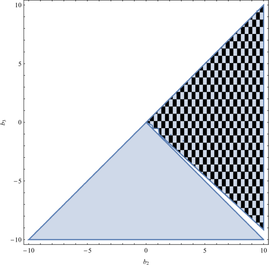
the critical density bigger than which is impossible) there is no physical third critical value for the density. The allowed parameter space which allows us to avoid this third critical value is depicted in Figure 11.
Figure 11: Region of parameters and which avoid the third critical value for the density. The region with the squared pattern corresponds to and the plain region to .
In order to impose on the model a non-singular behaviour at the Big Bang (BB), we concentrate on the first Friedmann equation (199) and require which means
(208)
so that we may write the first Friedmann equation in the following way
(209)
where will play the role of a maximum density as we know already from our analysis above.
To guarantee
that indeed has a minimum at the time when the Universe reaches , we must require .
We write this condition explicitly for the case
(210)
or equivalently,
(211)
Since , the condition of taken together with the inequality (208) can be translated into
(212)
On the other hand, for an accelerated evolution of the early universe we must look at the second Friedmann equation and require , at least for certain values of . For this to be possible, we see from equation (200) written now as
(213)
that the coefficient needs to be positive leading to the inequality
(214)
and constraining the density by
(215)
Note that for an accelerated expansion to occur, should be smaller than .
The above means that for an accelerated expansion to occur, must satisfy the inequality
(216)
We now have a full set of conditions for both the non-singular behaviour as well as an early accelerated expansion. This may be
interpreted in the following way: at a very early stage post Big Bang the density should lie in the region so that
it has an accelerated expansion. Later on, it will be in the region where there will be no more accelerated expansion
driven by spin terms.
Summarizing the scenario in this model we have
•
for a non-singular behaviour ()
(217)
(218)
•
For a consistent accelerating stage ()
(219)
In Figure 12 we have plotted the values of parameters and which fulfill all conditions (217), (218) and (219) simultaneously in the shaded region.
Figure 12: Region of parameters and for a non-singular and accelerated inflationary solution.
If we proceed to solve this model by using the continuity equation
we might introduce a singularity as it is evident by the following integral
(220)
which gives
(221)
This has to do with the third possible critical value of the density as shown previously, which might occur
if we do not put any further constraints on .
To avoid this possibility (and the possibility that the density will have several extrema)
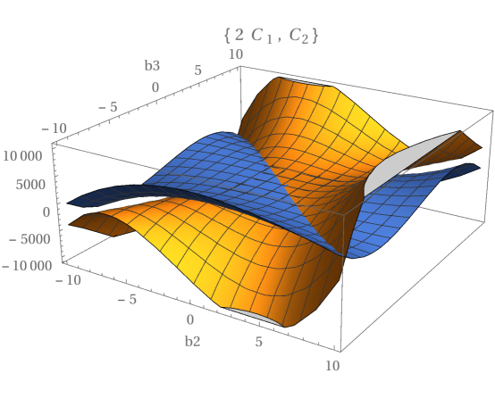
we insist on the consistency of (207), which implies . Since and are functions of and , then means that the surfaces described by intersect, as shown in Figure 13. The path of intersection may be written as
(222)
which is essentially a cubic equation in both and .
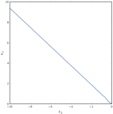
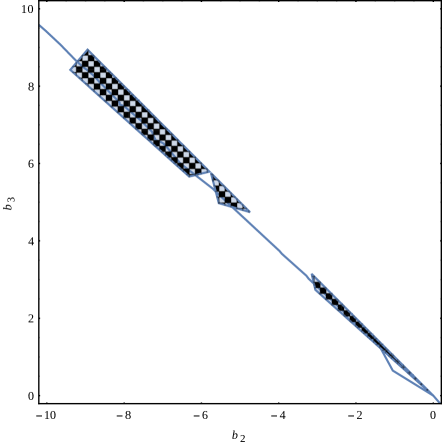
The region in which this equation is true turns out to resemble a line in the space parameter defined by and . This is shown in Figure 15 with the help of MATHEMATICA.
Figure 13: We plot consistent rescalings of (yellow) and (blue) as functions of and to show that the intersection between the two resembles a line. We show this in Fig. 15.
Figure 14: Plot of the values and which make the continuity equation consistent, namely the condition in equation (222). This corresponds to the intersection of the surfaces in Figure 13.
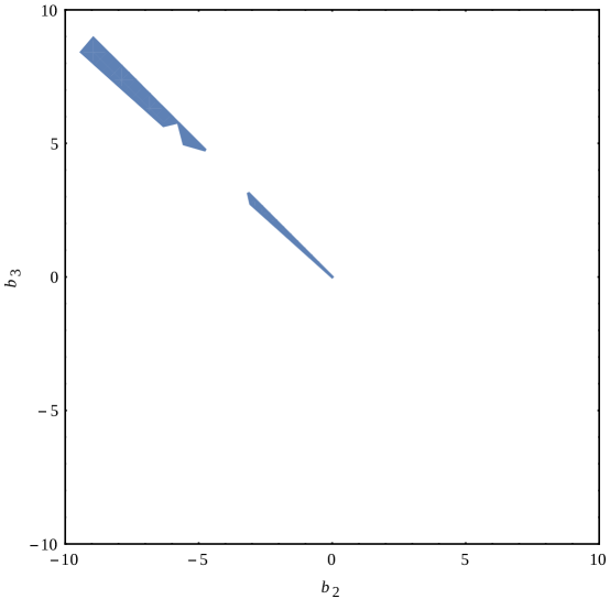
Figure 15: Combined plot of the values and which make the continuity equation ‘consistent’ (line plot) and those which yield also a non-singular and accelerated early universe (squared region).
We are left with the interesting possibility of exploiting certain values of and
in order to avoid initial singularity and have an inflationary phase. We plot these possible values in the combined Figure 15.
We mention that and , which would bring the Lagrangian into the
canonical form of Ricci scalar, is not a solution here. This is due to the fact that our model even for this particular choice of the
parameters differs from the standard Einstein–Cartan model in the identification, and hence choice, of the energy-momentum tensor.
The cosmology in the Einstein–Cartan theory based on the Lagrangian
proportional to the Ricci scalar but without the -terms will be singular as we have shown at the
end of section IV.
The scenario under discussion gets simplified since the continuity equation (202) may be written in a way analogous to GR, namely
(223)
(224)
which implies the usual GR result
(225)
This result can now be put into the first Friedmann equation to obtain the following integral
(226)
which is solved by
(227)
The plot of (227) is displayed in Figure 17 and it shows that it
is possible to reach a non-singular bounce-like behaviour for with .
Figure 16: Plot of both signs of equation (227) where it is clear to see that never reaches zero and that at its minimum value it has a smooth bounce.
Figure 17: Plot of both signs of equation (228) where it is clear to see that has a maximum value corresponding to , and that the branches seem to coincide smoothly at this value.
Using this solution for the form of can be obtained by replacing in terms of .
This gives
(228)
We plot this in Figure 17.
Alternatively, we could also solve numerically the equation
(229)
from which
(230)
The results agree with our previous method.
VII Different Averaging
A recent work Berredo on the issue of averaging the spin terms
claims a result different from the one we have discussed above.
The claim amounts to
(231)
We do not agree that this is the result obtained by Gasperini in Gasperini and stress that Gasperini has implicitly used the condition
. We think, however, that it may be worthwhile to check the implications of such an averaging on each
of the models presented before. Note that in the standard model discussed in section IV such a term cancels out so this model will not be modified by this change.
VII.1 Weyssenhoff perfect fluid with spin
We discuss below the alternative averaging for the model we outlined at the end of section IV where we dropped all terms proportional to .
Using the result given in equation (126) and considering
the modification given by the averaging results in equation (231), the new effective energy–momentum tensor is
(232)
This change modifies only the second Friedmann equation, resulting in the following set of equations
(233)
(234)
(235)
The continuity equation for the radiation case takes the form
(236)
Note that no critical densities are present. Solving for in terms of gives
(237)
The plot of (237) suggests a slightly modified behaviour with respect to standard General Relativity
but it still exhibits the standard behaviour as .
VII.2 Simplified alternative Lagrangian
In the case of the invariants , taking the different average will yield the following effective energy-momentum tensor in an analogous way to the previous
model, namely
(238)
which gives the Friedmann equations
(239)
(240)
The continuity equation for the radiation case is
(241)
We see again that the case with is rather uninteresting since it is a small generalization upon the first model. On the other hand, as we had before,
the case is indeed promising. For this case let us write this continuity equation in the form
(242)
with
(243)
We observe that again the first Friedmann equation defines a maximum density, namely
Thus, one of the effects of taking a different averaging is just to modify the numerical values of the
critical densities which satisfy the inequality
(244)
A similar relation was found before but now
(245)
At first glance it appears that may be positive. Taking yields for the radiation case
(246)
Hence, will be positive only if . The restrictions set by the
first Friedmann equation are sufficient. The different averaging only reflects in the change of and .
VII.3 General alternative Lagrangian
Using the set of invariants and its general Lagrangian, the different averaging
of equation (231) leads to the following effective energy–momentum tensor
(247)
which results in the following Friedmann equations
(248)
(249)
(250)
Note that as expected, the first Friedmann equation remains unchanged with respect to the Gasperini averaging Gasperini . This means that we can use the same
as defined in equation (196) but we need to define the following new constants
(251)
(252)
With these new constants the Friedmann equations will simplify as follows
(253)
(254)
We see that the same conditions apply for these coefficients as before, particularly the critical density is the same when , namely . The differential equation may be written in an analogous way using the dimensionless variables of equation (204) and one finds
(255)
The difference to the model we discussed before lies in the different values for .
VIII Conclusions and Outlook
In this paper we have examined in some detail the cosmological aspects of Einstein–Cartan theories
which allow an anti-symmetric part of the connection (contortion). Starting from the beginning, i.e. introducing the contortion
and relevant identities connected to it, we proceeded to the action principle based on the Lagrangian proportional to . We presented this
variation in two different manners to exhibit the one freedom which we have: the choice of the physical source. We argued that the latter can be
either the metric or the canonical energy-momentum tensor. We briefly discussed the standard approach with the canonical energy-momentum tensor
which essentially is imposed by us if we wish to have Einstein-like () equations for the metric.
The results are a bouncing universe with an inflationary expansion.
This approach is contrasted to a theory with the metric energy-momentum tensor where the determining equations are not canonical, i.e. not of the Einstein form.
In this set-up the theory resembles more the standard cosmology where the initial singularity cannot be avoided.
As a next step we have generalized the Lagrangian allowing for an arbitrary linear combination of diffeomorphic invariants. Based on these we constructed
two different cosmological scenarios. One with a finite non-zero bounce to be identified with a Big Bang and the other one describing a universe
born at finite non-zero value of the scale factor. We indicated possible acceleration of the expansion by a proper choice of the parameter space.
This shows that the cosmologies of the Einstein–Cartan type can have different cosmological consequences, but many of the versions share
the desirable feature of avoiding the initial singularity and possible having an accelerated early expansion. We find this a remarkable aspect of the
Einstein–Cartan cosmologies. More so as the extension of Einstein’s gravity to achieve this goal is rather mild and in many ways unconstrained as, for instance,
it does not alter any vacuum solutions. Notably the part of the torsion source can be identified with one of the
generators of the Poincaré–Lie algebra which is connected to the spin observable in the operator language. Here, obviously we can only talk about expectations values
and connect the spin expectation value to the expectation value of . Such an interpretation connects the source of the torsion directly with
quantum mechanics.
As we have demonstrated not all cosmological models based on the Einstein–Cartan theory lead to a singularity-free
cosmology (in the form a bounce). A thorough discussion of the connection between the bounce induced
by an anti-symmetric connection and the singularity theorems Chaubey ; Senovilla1
would be welcome. These singularity theorems are based on three assumptions: energy conditions (week, null, strong or
their averaged versions), causality condition and an initial boundary condition. In the past cosmologists
probing into bounces concentrated on the violation of one of the energy conditions, but the example of Senovilla’s
discovery Senovilla2 of a singularity-free solution with no violation of the energy and causality conditions
showed us that a more careful treatment is necessary. One of the first papers making a connection
between the absence of an initial cosmological singularity in theories with torsion and the singularity theorems
Kerlick also notices that in models with Dirac fields one finds an ’enhancement’ of the singularity formation.
In Pesmatsiou the authors point out that the weak energy condition is not always satisfied in
Einstein–Cartan spacetimes. Based on generalization of the singularity theorems Esposito reaches the conclusion
that in Einstein–Cartan spacetime the occurrence of singularities is less generic as compared to standard
General Relativity. The energy conditions (in particular the null one) are important for the wormhole solution
in theories with torsion Grezia .
Another interesting variant of the Einstein–Cartan theory not studied in this paper
is to include in the Lagrangian parity violating terms proportional to and examine in detail their cosmological implications ParityViolation concentrating on the aspects of the early universe.
Appendix A. Derivation of the contortion tensor
Demanding metricity when torsion is non vanishing fixes the behaviour of the contortion tensor in terms of the torsion
tensor. To get the contortion tensor we shall use the metricity condition, namely
(256)
(257)
(258)
Following Inverno , we consider the combination (256)+(257)-(258) and contract them with .
Furthermore, using leads to
(259)
(260)
where we have used .
Obviously this gives the symmetric part of the contortion tensor as
(261)
Adding its antisymmetric part the rearranged contortion tensor turns out to be
(262)
Appendix B. Standard FRLW cosmology approach
It is instructive to outline explicitly the differences of the models discussed above as compared to
the standard cosmological model which we briefly describe here.
We start from the following Friedman equation and the usual continuity equation
(263)
Now, in order to solve for in terms of we will first take the equation of state in the form and choose since we are
interested in the radiation dominated universe. From this we obtain
The result above implies that . Furthermore if
, then
blows up. Thus, grows faster as . We solve for
by using the first Friedmann equation we have written above. Since we have
(267)
then
(268)
the plots for these solutions are plotted in Figures 19 and 19.
Indeed, we see that if or
we obtain a divergent r.h.s. which implies a divergent
corresponding left hand side suggesting that either or . Since we have a freedom of choice, let us
assume that corresponds to the present epoch. This sets . It follows that the only value at which the
expression on the r.h.s. is divergent is taking on the l.h.s.
When solving for , we find
(269)
From equation (269)
we see that as , we plot both signs of this equation in Figure 21. This could in principle be associated with the
Big Bang time, so that the singularity can be associated to the ‘beginning’ of the Universe. To emphasize this, we take
and the solution can be written as
Moreover, given the expected Big Bang behaviour of the universe, it is evident we should assume an expanding early Universe, and thus, the in the solution
can be neglected by choosing the monotonically growing solution
(270)
This has also some implication upon since
(271)
Hence, the divergence of corresponds to the value .
The continuity equation allows to obtain in terms of by writing
(272)
This leads to
(273)
where is taken as the present value of the density of the universe, we plot this
behaviour in Figure 21.
The two different branches of the solution for cannot be glued together to arrive at a differentiable result.
Figure 18: Plot of the solution to equation (268). Observe that for a certain value of , goes to .
Figure 19: Plot of the solution to equation (269). Note that for a certain value of , goes either to zero or .
Figure 20: Plot the solution to equation (269). Observe that for , or to . Note that the positive value of the exponent corresponds to .
Figure 21: Plot of the solution to equation (271). Here, as .
Appendix C. Conservation laws
One can obtain conservation laws from identities obtained in ECKS theory. Let us start from equation (31)
When choosing in GR theory with the FLRW metric, one obtains the continuity equation . We expect an equivalent result considering the
energy–momentum identification as done in Hehl . This should match what we obtained in equation (105). We start with the r.h.s. of equation (31) for
(274)
since . Calculating the covariant derivative on the r.h.s. of (274) gives
(275)
where we have used the conditions and . We see that given the antisymmetry of only the antisymmetric
part of in the last term survives, that is .
On the other hand it is useful to write the expression as follows
(276)
where we have used the Christoffel Symbols for the FLRW metric.
Furthermore, the second term on the r.h.s. of (275) may be written as
(277)
We explore what happens to the Weyssenhoff term in
(278)
We note that the first term on the r.h.s. may be rewritten using
(279)
so that we finally obtain for the Weyssenhoff term
(8) W.G. Dixon, “Dynamics of extended bodies in general relativity. I. Momentum and angular momentum”, Proc. R. Soc. Lond. A 314 499, (1970)
(9) A. Papapetrou, “Spinning test-particles in general relativity. I” Proc. R. Soc. Lond. A 209 248, (1951).
(10) F.W. Hehl, P. von der Heyde, G. D. Kerlick and J.M. Nester, “General Relativity with Spin and Torsion: Foundations and Prospects”, Rev. Mod. Phys. 48 393, (1976).
(11) A. Trautman, “Spin and Torsion May Avert Gravitational Singularities”, Nature 242 7, (1973).
(12) A. Trautmann, “Einstein-Cartan Theory”, Encyclopedia of Mathematical Physics, edited by J.-P. Francoise, G.L. Naber and Tsou S.T. Oxford: Elsevier, 2 189, (2006).
(14) N.J. Popławski, “Cosmology with Torsion: An Alternative to Cosmic Inflation”, Phys. Lett. B694 181, (2010).
(15) I.L. Buchbinder, S. Odinstov and L. Shapiro, “Effective Action in Quantum Gravity”, Institute of Physics Publishing, (1992).
(16) H. I. Arcos and J. G. Pereira, “Torsion Gravity: a Reappraisal”, Int. J. Mod. Phys. D13 2193, (2004).
(17) C. G. Boehmer, “On Inflation and Torsion in Cosmology”, Acta. Phys. Polon. B36 2841, (2005).
(18) K. Pasmatsiou, C.G. Tsagas and J.D. Barrow, “Kinematics of Einstein-Cartan Universes”, Phys. Rev. D95 104007, (2017).
(19) R. D’Inverno, “Introducing Einstein’s Relativity”, Oxford University Press, (1998).
(20) C. W. Misner, K. S. Thorne and J. A. Wheeler, “Gravitation”, W. H. Freeman (1973).
(21) S. Weinberg, “Gravitation and Cosmology: Principles and Applications of the General Theory of Relativity”, John Wiley and Sons Ltd., (2013).
(22) J.A. Shouten, “Ricci Calculus”, Springer-Verlag, (1954).
(23) N.J. Popławski, “Spacetime and Fields”, arXiv:0911.0334 [gr-qc] (2009).
(24) F.W. Hehl, “Spin and Torsion in General Relativity: II. Geometry and Field Equations”, Gen. Relat. Gravit. 5 491, (1974).
(25) J. L. Safko, M. Tsamparlis and F. Elston, “Variational Methods with Torsion in General Relativity”, Phys. Lett. 60A 1, (1977).
(26) F.W. Hehl, “Spin and Torsion in General Relativity: I. Foundations”, Gen. Relat. Gravit. 4 333, (1973).
(27) F.W. Hehl, P. von der Heyde and G.D. Kerlick, “General Relativity with Spin and Torsion and its Deviations from Einstein’s Theory”, Phys. Rev. D10 1066, (1974).
(28) T. Ortín, “Gravity and Strings”, Cambridge Monographs on Mathematical Physics, (2004).
(29) L. L. Smalley, “Variational Principle for General Relativity with Torsion and Non-Metricity”, Phys. Lett. 61A 436, (1977).
(30) V. de Sabbata and C. Sivaram, “Spin and Torsion in Gravitation”, World Scientific (1994).
(31) W. Kopczyński, “An Anisotropic Universe with Torsion”, Phys. Lett. 43A 63, (1972).
(32) W. Arkuszewki, W. Kopczyński and V.N. Ponomariev, “On the Linearized Einstein-Cartan Theory”, Ann. Inst. Henri Poincaré 21 89, (1974).
(33) J. Weyssenhoff and A. Raabe, “Relativistic Dynamics of Spin-Fluids and Spin-Particles”, Acta Phys. Pol. 9 7, (1947).
(34) J.R. Ray and L.L. Smalley, “Improved Perfect-Fluid Energy-Momentum Tensor with Spin in Einstein-Cartan Space-Time”, Phys. Rev. Lett.49 1058, (1982).
(35) L.L. Smalley and J.R. Ray, “Weyssenhoff Spinning Fluid in Riemann-Cartan Spacetime: Direct Variation with Respect to the Spin Density of the Fluid”, Class. Quantum Grav. 7 1445, (1990).
(36) J.R. Ray and L.L. Smalley, “Equation-of-state spinning fluids in the Einstein-Cartan Theory”, Phys. Rev. D 35 1185, (1987).
(37) J.R. Ray and L.L. Smalley, “Spinning fluids in the Einstein-Cartan Theory”, Phys. Rev. D 27 1383, (1983).
(38) J.R. Ray and L.L. Smalley, “Spinning fluids in General Relativity”, Phys. Rev. D26 2619, (1982).
(39) J.R. Ray and L.L. Smalley, “Perfect Fluids in the Einstein-Cartan Theory”, Phys. Rev. D 26 2615, (1982).
(40) L.L. Smalley and J. P. Krisch, “Spinning Fluid Cosmologies in Einstein-Cartan Theory”, Class. Quantum Grav. 11 2375, (1994).
(41) L. L. Smalley, “On the Implications of Perfect Fluids in Metric-Affine Spacetime”, Class. Quantum Grav. 17 1447, (2000).
(42) J.R. Ray, L.L. Smalley and J.P. Krisch, “Spinning Fluids in General Relativity. II. Self-consistent Formulation” Phys. Rev. D 35 3261, (1987).
(43) J. Frenkel, “ Über die Wärmebewegung in Festen und Flüssigen Körpern”, Z. Physik 35 652, (1926).
(45) N. J. Popławski, “Universe in a Black Hole with Spin and Torsion”, ApJ. 832 96, (2016).
(46) M. R. Mehdizadeh and A. H. Ziaie, “Einstein-Cartan Wormhole Solutions”, Phys. Rev. D 95 064049, (2017).
(47) Y. N. Obukhov, “Spinning Fluid in General Relativity”, Class. Quantum Grav. 6 L15, (1989).
(48) Y. N. Obukhov and V.A. Korotky, “The Weyssenhoff Fluid in Einstein-Cartan Theory”, Class. Quantum Grav. 4 1633, (1987).
(49) J. B. Bjorken and S. D. Drell, “Relativistic Quantum Fields”, McGraw-Hill, (1965).
(50) M.O. Ribas and G.M. Kremer, “Fermion Fields in Einstein-Cartan Theory and the Accelerated-Decelerated Transition in a Primordial Universe” Gravit. Cosmol. 16 173, (2010).
(51) C.F. Diether and J. Christian, “On the Role of Einstein-Cartan Gravity in Fundamental Particle Physics” arXiv:1705.06036 [gr-qc] (2017).
(52) T. W. Kibble, “Lorentz Invariance and Gravitational Field”, J. Math. Phys. 2, 212 (1961).
(53) F. W. Hehl and B. K. Datta, “Nonlinear Spinor Equation and Asymmetric Connection in General Relativity”, J. Math. Phys. 12,
1334 (1971).
(54)
S. Farnsworth and J.-L. Lehners, “Spinor driven Cosmic Bounces and Their
Cosmological Pertubations”, Phys. Rev. D96, 083530 (2017).
(55)
J. M. Weller, “Fermion Condensate from Torsion in the reheating Era after
Inflation”, Phys. Rev. D88, 08354 (2013).
(56)
N. J: Popławski,
“Matter-Antimatter Asymmetry and Dark Matter from Torsion”,
Phys. Rev. D83, 084033 (2011).
(57)
N. J. Popławski, “”Cosmological Constant from Quarks and Torsion”,
Annalen der Physik (berlin), 523 (2011)
(58)
N. J. Popławski, “Four-Fermion Interaction from Torsion as Dark Energy”,
Gen. Relat. Gravit. 44, 491 (2012).
(59)
J. Boos and F. W. Hehl. “Gravity-Induced Four-Fermion
Contact Interaction Implies Gravitational Intermediate W and Z Type Gauge
Bosons”, Int. J. Theor. Phys. 56, 751 (2017).
(60) R. de Ritis, M. Lavorgna, G. Platania and C. Stornaiolo, “Spin Fluid in Einstein-Cartan Theory: A Variational Principle and an Extension of the Velocity Potential Representation”, Phys. Rev. D28 713, (1983).
(61) K. Atazadeh, “Stability of the Einstein static Universe in Einstein-Cartan theory”, JCAP06 020, (2014).
(62) S. M. Carroll, “Spacetime and Geometry: An Introduction to General Relativity”, San Francisco: Addison Wesley, (2004).
(63) A. Ashtekar and P. Singh, “Loop Quantum Cosmology: A Status Report”, Class. Quant. Grav. 28 213001, (2011).
(64) A.F. Ali and B. Majumder, “Towards a Cosmology with Minimal Length and Maximal Energy”, Class. Quant. Grav. 31, 215007 (2014).
(65) P. Bargueño, S. Bravo–Medina, M. Nowakowski and D. Batic, “Newtonian Cosmology with a Quantum Bounce” Eur. Phys. J. C 76, 543 (2016); P. Bargueño, S. Bravo–Medina, M. Nowakowski and D. Batic, “Quantum Mechanical
Corrections to the Schwarzschild black-hole metric”, EPL 117 60006 (2017).
(66) I.S. Nurgaliev and W.N. Ponomariev, “The Earliest Evolutionary Stages of the Universe and Space-Time Torsion”, Phys. Lett. 130B 378, (1983).
(67) Y. N. Obukhov, “Spin-Driven Inflation”, Phys. Lett. A182 214, (2000).
(68) M. Gasperini, “Spin-Dominated Inflation in the Einstein-Cartan Theory”, Phys. Rev. Lett. 56 2873, (1986).
(69) F. Lucchin and S. Matarrese, “Power-law Inflation”, Phys. Rev. D32 1316, (1985).
(70) F. Lucchin and S. Matarrese, “Kinematical Properties of Generalized Inflation”, Phys. Lett. B164 282, (1985).
(71) A. Guth, “Inflationary Universe: A possible solution to the
horizon and flatness problems” Phys. Rev. D23 347, (1981).
(72) A.R. Liddle, “Power-law Inflation with Exponential Potentials”, Phys. Lett. B 220 502, (1989).
(73) N.J. Popławski, “Big Bounce from Spin and Torsion”, Gen. Relativ. Gravit. 44 1007, (2012).
(74) H.P. de Oliveira, “Spinning Fluids in the Eistein-Cartan Theory: a Variational Formulation”, Gen. Relat. Gravit. 25 473, (1993).
(75) A.H. Ziale, P.V. Moniz, A. Ranjbar and H.R. Sepangi, “Einstein-Cartan Gravitational Collapse of a Homogeneous Weyssenhoff Fluid”, Eur. Phys. J. C 74 3154, (2014).
(76) R. Aldrovandi and J.G. Pereira, “Teleparallel Gravity”, Springer, (2013).
(77) J.W. Maluf, “The Teleparallel Equivalent of General Relativity”, Annalen der Physik 525 339, (2013).
(78) K. Hayashi and T. Shirafuji, “New General Relativity” Phys. Rev. D19 3524, (1979).
(79) G. Otalora, “A novel Teleparallel Dark Energy Model”, Int. J. Mod. Phys. D25 1650025, (2016).
(80) Y-F. Cai et al., “ Teleparallel Gravity and Cosmology”, Rept. Prog. Phys. 79 106901, (2016).
(81) A. Golovnev, T. Koivisto and M. Sandstad, “On the covariance of Teleparallel Gravity theories”, Class. Quant. Grav. 34 145013, (2017).
(82) G. de Berredo-Peixoto and E.A. de Freitas, “On the Torsion effects of a Relativistic Spin Fluid in Early Cosmology”, Class. Quant. Grav. 26 175015, (2009).
(83) T. Singh, R. Chaubey and A. Singh, Bounce conditions For FRW models in modified gravity theories”, Eur. Phys. J. Plus
130, 31 (2015).
(84) J. M. M. Senovilla, “Singularity Theorems and Their Consequences”, Gen. Relat. grav.30, 701 (1998).
(85) J. M. M. Senovilla, “New class of inhomogeneous cosmological perfect-fluid solutions without
big-bang singularity”, Phys. Rev. Lett. 64, 22191 (1990).
(86)G. D. Kerick, “Bouncing of Simple Cosmological Models with Torsion”, Ann. Phys. 99, 127 (1976).
(87)K. Pesmatsiou, Ch. G. Tsagas and J. D. Barrow, “Kinematics of Einstein-Cartan universes”,
Phys. Rev. D95, 104007 (2017).
(88) G. Esposito, “The Singularity Problem for Space-Times with Torsion”, Nuovo Cimento B105, 75
(1990).
(89) E. Battista, E. Di Grezia. M. Manfredonia and G. Miele, ‘Spin, Torsion and Violation of Null
Energy Condition in Traversable Wormholes”, Eur. Phys. J. Plus 132, 537 (2017).
(90) R. Hojman, C. Mukku and W.A. Sayed, “Parity Violation in Metric-Torsion Theories of Gravitation”, Phys. Rev. D 22 1915, (1980).