Physics and Astrophysics of Strong Magnetic Field systems with eXTP

Abstract

In this paper we present the science potential of the enhanced X-ray Timing and Polarimetry (eXTP) mission for studies of strongly magnetized objects. We will focus on the physics and astrophysics of strongly magnetized objects, namely magnetars, accreting X-ray pulsars, and rotation powered pulsars. We also discuss the science potential of eXTP for QED studies. Developed by an international Consortium led by the Institute of High Energy Physics of the Chinese Academy of Sciences, the eXTP mission is expected to be launched in the mid 2020s.

47.55.nb, 47.20.Ky, 47.11.Fg

1 The eXTP mission

In this white paper we present the science potential of the enhanced X-ray Timing and Polarimetry (eXTP) mission for studies of strongly magnetized objects. The scientific payload of eXTP consists of four main instruments: The Spectroscopic Focusing Array (SFA), the Polarimetry Focusing array (PFA), the Large Area Detector (LAD) and the Wide Field Monitor (WFM). A detailed description of eXTP ’s instrumentation, which includes all relevant operational parameters, can be found in [1], but we summarize it briefly here.

The SFA is an array of nine identical X-ray telescopes covering the energy range 0.5-10 keV, featuring a total effective area of 0.4 m² at 6 keV, and close to $\sim 0.5$ m² at 1 keV. The SFA angular resolution is $\sim 1$ arcmin and its sensitivity reaches $10^{-14}$erg s^-1 cm^-2 for an exposure time of $10^{4}$ ks. In the current baseline, the SFA focal plane detectors are silicon-drift detectors (SDDs), which combine CCD-like spectral resolution with very short dead time and a high time resolution of 10$\mu$s; they are therefore well-suited for studies of the brightest cosmic X-ray sources at the shortest time scales.

The PFA consists of four identical telescopes, with angular resolution better than $\sim 30$ arcsec and total effective area of $\sim 700$ cm² at 2 keV (including the detector efficiency), featuring Gas Pixel Detectors (GPDs) to allow polarization measurements in the X-rays. The PFA is sensitive in the 2-8 keV energy range, and features a time resolution better than 500$\mu$s. The instrument reaches a minimum detectable polarization of 5% in 100 ks for a Crab-like source of flux $10^{-11}$erg s^-1 cm^-2.

The LAD has a very large effective area of $\sim 3.4$ m² (at 6 keV), obtained with non-imaging SDDs, active between 2 and 30 keV and collimated to a field of view of 1 degree across. It features absolute timing accuracy of $\sim 1\mu$s, and an energy resolution better than 260 eV (at 6 keV). The LAD and the SFA together reach an unprecedented total effective area of $\sim 4$ m².

The science payload is completed by the WFM, consisting of 6 coded-mask cameras covering more than 3.2 sr of the sky at a sensitivity of 4 mCrab for an exposure time of 1 d in the 2 to 50 keV energy range, and for a typical sensitivity of 0.2 mCrab combining 1 yr of observations outside the Galactic plane. The instrument will feature an angular resolution of a few arcmin and will be endowed with an energy resolution of about 300 eV.

Developed by an international Consortium led by the Institute of High Energy Physics (IHEP) of the Chinese Academy of Sciences, the mission is expected to be launched around 2025. In section §2 we focus on the eXTP science potential for magnetar candidates, namely the anomalous X-ray pulsars (AXPs) and soft gamma ray repeaters (SGRs). In section §3 we discuss the eXTP capability for accreting and rotation powered pulsars. Finally, in section §4, we present the expected eXTP impact on QED studies.

2 The physics and astrophysics of AXPs/SGRs as magnetar candidates

2.1 Introduction

Pulsars are rotating magnetized neutron stars (NSs), and are amongst the most fascinating objects in astrophysics due to their potential as laboratory for physics under extreme conditions. Their periodic modulation reflects their rotation period. They appear in many flavors and show a rather different phenomenology depending on key parameters such as the spin period and magnetic field intensity. The spin period and period derivative of different types of pulsars are shown in Figure 1 together with lines of constant B-field characteristic age $\tau$ (see e.g., [2] for a review). Several classes can clearly be identified, including the class of magnetars on the top right of the figure.

Magnetars are NSs with extremely intense magnetic fields of the order of B$\sim$10^14-15 G [3, 4], whose decay or recombination powers their high energy emission in X-rays and even gamma rays. Magnetars are thought to manifest as anomalous X-ray pulsars (AXPs) and soft gamma repeaters (SGRs), with spin periods of $\sim(1-10)$ s and period derivatives of $\sim(10^{-15}-10^{-10})\leavevmode\nobreak\ {\rm s/s}$.

From X-ray observations, nearly thirty magnetar candidates have been identified so far.

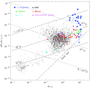
Figure 1: Period and period derivative diagram of neutron stars, including normal pulsars (black points), magnetars (blue squares, empty squares for radio loud magnetars), X-ray dim isolated neutron stars (green diamonds), central compact objects (light blue circles), rotating radio transients (red stars) and intermittent pulsars (magenta triangles) [6].

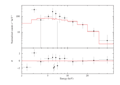
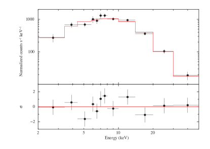
Figure 2: Left: Simulated WFM spectrum of a magnetar burst (black points) for a 0.05 s burst duration, assuming a flux of 10 Crab (left) and 150 Crab (right), and a double blackbody spectrum.

AXPs/SGRs feature energetic events not seen in most pulsars. They emit short bursts of X-rays and soft $\gamma$-rays, which often reach super-Eddington luminosities. More rarely, they also exhibit intermediate (IFs) and giant flares (GFs), involving the release of up to $10^{46}\leavevmode\nobreak\ {\rm erg}$ in less than half a second. AXPs/SGRs are also sources of persistent pulsed X-ray emission with typical luminosity of $\sim 10^{35}\leavevmode\nobreak\ {\rm erg/s}$.

They are ideal targets for eXTP, since the broad band, high sensitivity, polarimetric and monitoring capability of the mission will lead to the prompt discovery of outbursts from known and new sources, thus enabling deep studies of magnetar phenomenology on different time scales.

In fact, eXTP will have an unprecedented capability to study their bursts, outbursts (§2.2), and their timing behaviour (§2.3), including glitches and precession. eXTP observations will allow us to measure braking indices in a more reliable way, and to perform asteroseismology. Phase dependent absorption spectral features could also be observed systematically by eXTP, enabling investigations of the intensity and topology of the magnetic field configuration in the vicinity of the NS (§2.4). Furthermore, a combined study of spectra, timing and polarization may result in key detections of magnetars in binary systems. All of these are essential studies to unveil the nature of magnetars and to answer long-standing open questions in magnetospheric and fundamental physics. (§2.5).

2.2 Bursts and Outbursts

Magnetars are highly variable X-ray sources, with the flux changing by as much as a factor of thousand. Variability occurs on different times scales, e.g. short bursts ($<1$ s), intermediate flares ($1-40$ s), giant flares ($\sim$500 s), and outbursts that can last several weeks to years.

Indeed, most magnetar candidates were discovered thanks to their bursting and transient X-ray emission by previous wide field monitors such as the Fermi’s GBM and the Burst Alert Monitor on Swift. Giant flares are very rare events and have not been observed to repeat in a single source. Both bursts and intermediate flares can recur on a time scale of a few hours.

2.2.1 Burst Emission: spectral and polarization properties

Magnetar bursts show a variety of spectral and timing behaviors [8].

The emission process is generally assumed to be initiated by rapid rearrangements of the magnetic field, possibly involving either induced or spontaneous magnetic reconnection. This accelerates charged particles with ensuing gamma-ray emission, since the rapid acceleration of electrons in a strongly curved field leads to a cascade of pair creation and gamma-rays [7]. However, fully self-consistent models of the emission resulting from the various proposed trigger mechanisms do not yet exist. Considering their variability time scales and the WFM sky coverage, eXTP may discover a new candidate magnetar every year, triggering follow-up observations with the eXTP narrow field instruments and other facilities. These follow-up observations of bursts and IFs are crucial to inferring the NS’s interior properties (see §2.3.4) and to search for proton cyclotron resonance scattering features (CRSF) in the X-ray spectrum (e.g., [10], see §2.4).

Figure 3: Simulated LAD spectrum of a magnetar burst (black points) for a 0.05 s burst duration, assuming a flux of 10 Crab, a double blackbody spectrum, and an absorption feature at 4.5 keV (200 eV EW). The red line in the top panel shows the best-fit model obtained assuming a double blackbody spectrum. The lower panel shows the residuals with respect to the best-fit model, when the CRSF is not included.

Assuming a 0.05 s burst duration, a peak flux of 150 Crab, and a spectrum consisting of two absorbed blackbodies with $kT_{1}=5.4$ keV, $kT_{2}=10.2$ keV and $N_{H}=2.1\times 10^{22}$ cm^-2 (as in the event observed from SGR 1900+14, [11]), we obtain a WFM count-rate of $(1.40\pm 0.05)\times 10^{4}$ cts s^-1, showing that such a burst will be detected with high significance (see Fig 2).

The fit of a simulated LAD spectrum of a much fainter burst of 10 Crab with a proton cyclotron resonant scattering feature (CRSF) at 4.5 keV, and equivalent width of 200 eV (shown in Fig 3), shows that these absorption features can be detected with a high significance (at more than 8$\sigma$) within a single burst. These features will be discussed in detail in §2.4.

In order to test eXTP’s ability to measure polarization properties of magnetar bursts, we have produced several simulated data sets, using for the burst the model recently developed by [8]. The burst spectral and polarization properties were computed within the fireball scenario developed by [9], both in the case in which the pair plasma fills the entire toroidal region limited by a set of closed field lines (model a), and in the case where the emitting region is confined to a portion of the torus-like volume (model b). Simulations were performed for a typical intermediate flare, like those emitted by SGR 1900+14 during the “burst forest” of 2006 [11], with duration $\sim 1.7$ s and $1$–$10$ keV flux $\sim 5\times 10^{-7}\ {\rm erg/cm^{2}/s}$. Results are shown in Fig 4.

Both polarization fraction and angle measurements recover, within $1\sigma$ uncertainties, values used in the simulations. It should be noted that although the errors on the polarization fraction are more or less the same for all the geometrical configurations considered, those on the polarization angle increase by decreasing the corresponding degree of polarization. Instrumental effects only dominate the polarization angle measurements for $P\lesssim 20\%$.

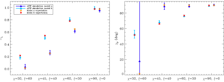
Figure 4: Simulated polarization fraction (left panel) and angle (right panel) as measured by the eXTP polarimeter for an intermediate burst computed according to model a (orange crosses) and model b (red crosses) of [9]; the simulated eXTP response is shown by the light-blue and dark-blue triangles, respectively, with 1$\sigma$ error bars. An exposure time of 1.737 s (i.e. the total duration of the burst) is assumed, together with a $1$–$10$ keV flux of $4.68\times 10^{-7}$ erg/cm²/s. The simulations are performed for different values of the geometrical angles $\chi$ and $\xi$, which represent the inclination of the line-of-sight and of the magnetic axis with respect to the rotation axis, respectively.

2.2.2 Outbursts’ Decay

The largest amount of physical information on magnetars is gathered during outbursts, when the emission is enhanced at all wavelengths and the variability is rapid, challenging our present knowledge of heating mechanisms and NS thermal inertia. During outbursts, the X-ray flux of the source suddenly increases by a factor $\sim(10-1000)$ over the persistent level in a few hours. During the active phase, which lasts $\sim 1$ year, the flux declines, the spectrum softens and the pulse profile simplifies. Since such outbursts are likely produced by deformations of the neutron star crust, which, in turn, produce a rearrangement of the external magnetic field over a large scale [12], dedicated observational campaigns of transient sources offer the best opportunity to monitor the evolution of the magnetosphere at different luminosities and at high spectral resolution, over several months/years.

The LAD and SFA can monitor the light curve, pulse profiles and spectra over a broad energy range, from a few hours after the onset of the outburst to its decay to the quiescent state, at a level of precision unattainable by NuSTAR [13].

The combination of eXTP instruments will enable us to study the correlation between variabilities in at least two bands, and will reveal the slope turn-over in the soft-to-hard emission, generating a deep understanding of the magnetic field and current distributions. eXTP phase-resolved spectroscopy will allow us to track the variability of the magnetospheric configuration during the outburst decay, following the variations in the power-law spectral component, and to search for CRSF variability. For objects that reach surface temperatures as high as $\sim 1$ keV, phase-resolved spectroscopy will also allow us to map the region of the NS surface heated during the early phases of the outburst.

A unique and unprecedented characteristic of eXTP is that it will perform timing and polarization measurements simultaneously. The change of the angle and degree of polarization during the outburst, combined with measurements of flux and spectral evolution, will yield a unique and novel data set to constrain the magnetospheric topology and remove existing degeneracies in proposed models [14].

Data will also allow us to compare detailed predictions from the twisted magnetosphere and thermal relaxation models: different polarization signatures are expected, depending on which effect dominates, and quantitative theoretical studies are presently in progress. Furthermore, polarimetric measurements of the thermal X-ray component of transient magnetars during an outburst decay will provide a crucial tool to prove magnetospheric untwisting and in turn to test the magnetar scenario for the post-outburst relaxation epoque, as shown later in sec. 4.2, and in [15, 16].

2.3 Timing Properties

Thanks to the large field of view of the WFM, a large fraction of the Galactic Plane (where most magnetar candidates have been discovered) will be covered during most eXTP pointings. This gives us the possibility of monitoring the spin period of several magnetars simultaneously, to obtain phase-connected timing solutions. For X-ray fluxes of a few mCrab, the WFM will accurately measure magnetar pulsations in a few tens of ks. We note that all of the persistently bright magnetars are radio quiet and hence X-ray timing is the only way of measuring their spin evolution. Via the monitoring of the spins, we will be able to detect glitches, possibly reveal precession, and accurately measure braking indices, as well as other timing irregularities. We can investigate whether these events anticipate bursts or giant flares. The dramatic increase in the effective area provided by LAD/SFA in comparison to previously flown missions is also likely to reveal new timing features. The observed timing behaviors could provide valuable information about the physical mechanism of energy release and the radiative process.

2.3.1 Glitches

Magnetars (AXPs and SGRs) show peculiar timing behaviors, with frequent glitches and occasional anti-glitches [17]. The fractional change in the spin frequency is typically $\Delta{\nu}/{\nu}\sim(10^{-7}-10^{-4})$ for AXPs/SGRs, similar to that observed during large glitches in radio pulsars. The lack of smaller glitches reflects the limited observational capability of X-ray facilities, due to the combined effect of the larger timing noise of magnetars compared to radio pulsars and the lower cadence of timing observations [18, 19]. The glitches are usually (but not always) accompanied by X-ray flux enhancement. Notably, SGR 1900+14 and 1E 2259+586 experienced events in which the spin frequency jumps to a value smaller than that predicted by the observed spin-down rate (with negative $\Delta\nu$, as for anti-glitches). Within the conventional magnetar model, the problem of fully understanding glitches (with or without X-ray enhancement) is still challenging. Several explanations have been proposed, including collision with small solid bodies [20], emission of enhanced particle winds [21], and starquakes in a solid strangeon star [22, 23]. In order to test these models, it is necessary to detect glitches at the extremes of their amplitude, i.e. either very large or very small. As shown in Fig. 5, simulations indicate that in a source as 4U 0142+61, eXTP could detect a glitch/antiglitch with amplitude $\Delta\nu/\nu\sim 10^{-8}\leavevmode\nobreak\ \rm{s/s}$ in about 250 d assuming 2 ks monitoring observations with a two week cadence. Furthermore, eXTP observations will allow us to detect or rule out X-ray enhancement during a small glitch (see the bottom panel of Fig. 5). This is extremely important since the smaller glitches/antiglitches could put tighter constraints on the various timing anomaly mechanisms if no faint X-ray outbursts occur.

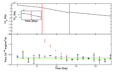
Figure 5: eXTP simulation of a small glitch with/without X-ray outburst. The input spectrum is a combination of a blackbody and a power law, absorbed at lower energies. The hydrogen column density, the blackbody temperature and its normalization are $0.95\times 10^{22}\leavevmode\nobreak\ {\rm cm^{-2}}$, $0.395\leavevmode\nobreak\ {\rm keV}$ and $0.1558$, respectively. Points indicate observations of 2 ks spaced by intervals of 2 weeks, hence the total exposure time is $3.34\times 10^{4}\leavevmode\nobreak\ \rm{s}$. In the bottom panel, the red data show the X-ray outburst during a small glitch, while the black data represent the persistent emission.

2.3.2 Precession

In the magnetar model it is expected that strong dipolar and multipolar magnetic fields could induce large stresses on the star, in turn inducing significant distortions of the star’s shape. As a consequence, free precession of the NS may manifest as a modulation of the spin frequency [24]. Such a modulation has not yet been firmly observed. Nevertheless, possible evidence for magnetar precession has been suggested from the analysis of X-ray phase modulations [25]. The time scale of free precession is inversely proportional to the square of the internal magnetic field $B_{\rm in}$,

$$\tau_{\rm pr}={2\pi\over\epsilon\Omega}\simeq 2\times 10^{-2}\left({B_{\rm in}\over 100B_{\rm QED}}\right)^{-2}\left({P\over 6{\rm s}}\right)\leavevmode\nobreak\ {\rm yr},$$ (1)

where $B_{\rm QED}=4.414\times 10^{13}$ G is the quantum critical field. A firm detection of precession would have several implications for superconductivity in magnetar interiors [26, 27]. On the other hand, if some of the alternative models that suggest AXPs and SGRs host normal magnetic fields with $B_{\rm in}\sim 10^{12}$ G, are correct, precession might not necessarily occur, either because the time-scale would be too long or because the deviation from spherical symmetry in the compact star (with mass $\sim M_{\odot}$) would be negligible, e.g., [28]. eXTP will search for precession in AXPs/SGRs, ultimately testing the magnetar model and constraining the star’s parameters. As shown in Figure 6, systematic temporal monitoring with eXTP will allow us to detect the amplitude of free precession down to a level of $\Delta\nu\sim 10^{-9}\leavevmode\nobreak\ {\rm Hz}$, in a magnetar like SGR 1900+14.

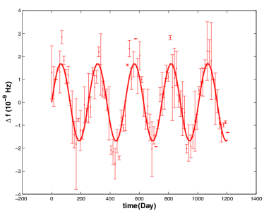
Figure 6: eXTP simulation of free precession in SGR 1900+14. The input spectrum is a blackbody plus a power law, with low energy absorption. The hydrogen column density, the blackbody temperature and its normalization for SGR 1900+14 are $1.6\times 10^{22}\leavevmode\nobreak\ {\rm cm^{-2}}$, 0.5 and 7.1 keV, respectively. The sinusoidal modulation of the free precession is assumed. Points indicate observations of 2 ks spaced by intervals of 2 weeks, hence the total exposure time is $1.15\times 10^{5}\leavevmode\nobreak\ \rm{s}$.

2.3.3 $\ddot{\nu}$ and braking index of magnetars

The braking index $n$ of pulsars is defined as

$$n=\frac{\nu\ddot{\nu}}{\dot{\nu}^{2}},$$ (2)

where $\dot{\nu}$, and $\ddot{\nu}$ are the pulse frequency derivative, and frequency second derivative, respectively. The braking index reflects the physics of the pulsar spin-down torque, through its effect on the angular velocity. To date, 8 pulsars have a measured braking index [29], and more than 300 pulsars have a second derivative of the frequency reported [30]. However, the frequency second derivatives of these pulsars may be dominated by timing noise. For 17 magnetars the second derivative of the frequency has been reported. Among them, 7 show a positive $\ddot{\nu}$, while the other 10 systems have a negative $\ddot{\nu}$. Furthermore, the frequency second derivatives of pulsars and magnetars are correlated with their spin-down rate, as shown in Fig. 7. There are at least three causes that may contribute to the $\ddot{\nu}$ observed in magnetars. They are, in order of decreasing importance:

1. Fluctuations in the magnetosphere. This process may in fact dominate the currently observed $\ddot{\nu}$ in magnetars and pulsars and also explain the observed correlation (see again Fig. 7). The corresponding second derivative is given by  [31] as

   $$|\ddot{\nu}|=2\pi\delta\frac{|\dot{\nu}|}{T},$$ (3)

   where $\delta$ and $T$ are the typical amplitude and timescale of the magnetospheric fluctuations.

2. A decreasing spin-down rate, due to a decreasing particle wind in the magnetosphere [32, 33]. This process naturally explains a corresponding positive $\ddot{\nu}$. However, the predicted magnitude is about an order of magnitude smaller than the actual observed values.

3. A braking index about one. Again, the corresponding values of $\ddot{\nu}$ (from equation 2) are several orders of magnitude smaller than the current observed values.

Since the quiescent states of transient magnetars are less noisy, more accurate timing during the quiescent state may reveal the $\ddot{\nu}$ corresponding to a decreasing spin-down rate/wind or, at least for some sources, may allow us to test the determination of the braking index. eXTP’s LAD has larger detection area, and thus is more effective in timing of magnetars in the X-ray band. This will permit us to conduct regular monitoring of spin frequency changes for a sample of sources using comparatively short exposures, and thus constrain the braking index in more sources.

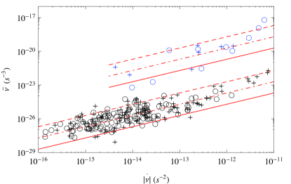
Figure 7: $\ddot{\nu}$ versus $\dot{\nu}$ for pulsars and magnetars. Black ‘+’ stands for pulsars with postive $\ddot{\nu}$ and black ‘$\circ$’ for negative $\ddot{\nu}$. Blue ‘+’ and ‘$\circ$’ are for magnetars. The lines are model calculations with different fluctuation amplitude. Updated from Figure 9 in [31].

2.3.4 Asteroseismology

In the era of CoRoT and Kepler, seismology has become firmly established as a precision technique for the study of stellar interiors. The detection of seismic vibrations in NSs was one of RXTE’s most exciting discoveries, as it allows a unique, direct view of the densest bulk matter in the Universe. Vibrations, detectable as quasi-periodic oscillations (QPOs) in the hard X-ray emission, were found in the tails of giant flares from two magnetars [34, 35, 36, 37]. Other candidate QPOs have since been discovered during storms of short, low fluence bursts from several magnetars [38, 39, 40]

Seismic vibrations from magnetars can in principle tightly constrain both the interior magnetic field strength (which is hard to measure directly) and the EOS [41, 42]. They can also go beyond the EOS, constraining the non-isotropic components of the stress tensor of supranuclear density material. Seismic oscillation models now include the effects of the strong magnetic field that couples crust to core in magnetars [43, 44, 45, 46, 47, 48], superfluidity, superconductivity and crust composition [49, 50, 51, 52]. More sophisticated models are under development, and much of the current effort is focused on numerical implementation.

With its large collecting area and excellent timing resolution, eXTP would be ideally placed to find QPOs in magnetar GFs, should one occur during the mission lifetime. However, they are rare events, occurring only once every $\sim$ 10 years. What makes eXTP unique is that it will be sensitive to QPOs of less bright (but still $\sim 10^{3}$ Crab) IFs, which occur much more frequently. IFs have similar peak fluxes as the tails of the GFs, but are too brief ($\sim 1$ s) to permit detection of similar QPOs with current instrumentation. Figure 8 shows a simulation of the power-spectrum of the IF observed from SGR 1900$+$14 in 2006, as seen by eXTP. We artificially added to the simulated lightcurve several QPOs at frequencies similar to those observed in magnetar GFs (i.e. all those detected in the GF of SGR 1806$-$20 plus few additional ones), using a fractional rms amplitude of 2, 1, and 0.5 in units of the rms amplitude observed in the GF. Simulations indicate that the LAD onboard eXTP will be able to detect QPOs in IFs down to an amplitude of 0.5 of that observed in the GFs, using only data from a single IF, without the need to stack several events. Although the reported simulation is valid for events detected on-axis, we expect that – depending on the flux level of the IF – it will be possible to perform a detection at a similar level in bursts detected off-axis. Both IFs and GFs are in fact more likely to be observed off-axis due to their unpredictability. Depending on the collimator properties, we expect a limited reduction in sensitivity, of the order of $\sim 30$%, for off-axis detections (detailed simulations for off-axis events are underway and will be reported in due course). In addition, eXTP can make pointed observations of bursting magnetars when they enter an active phase (when bursting frequency increases) to detect many short, low fluence bursts. Applying the techniques of [38], and stacking bursts together, it will be possible to detect vibrations during magnetar burst storms.

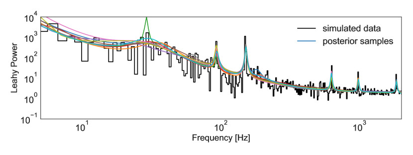
Figure 8: Black: simulated LAD eXTP data of the lightcurve of the IF observed from SGR 1900$+$14 in 2006, with quasi-periodic oscillations at 30 Hz, 92 Hz, 150 Hz, 625 Hz, 976 Hz, and 1840 Hz, at a fractional rms amplitude of $50\%$ (with respect to that observed from the GF of SGR 1806$-$20). Overplotted in color are ten realizations from the posterior distribution of a mixture model of Lorentzian components, clearly identifying all but the lowest-frequency QPO present in the data.

2.4 Spectral lines

Tiengo et al. (2013) [53] reported the discovery of a phase-variable absorption feature in the X-ray spectrum of SGR 0418+5729. The feature was best detected in a 67 ks XMM-Newton observation performed on August 2009, when the source flux was still particularly bright ($5\times 10^{12}$ erg cm² s^-1 in the 2-10 keV band). It has also been detected in RXTE and Swift data obtained in the first two months after the outburst onset. The line energy lies in the range 1-5 keV and changes sharply with the pulse phase, by a factor of $\sim 5$ in one-tenth of a cycle.

The most viable interpretation is in terms of a proton CRSF produced in a baryon-rich magnetic structure (a small loop) localised close to the NS surface [54]. The energy of proton CRSF scales linearly with the magnetic field as $E_{p}\sim 0.44B_{14}$ keV (assuming a standard NS EOS) and thus, for fields in the magnetar range, they are expected to be observed below $\sim 6$ keV.

If the proton CRSF interpretation is correct, the presence of the line probes the complex topology of the magnetar magnetic field close to the surface and provides evidence of multipolar components of the star’s magnetic field. This strengthens the idea that magnetar bursting behavior is dictated by high magnetic fields confined near the surface/inside the crust rather than by the large scale magnetic dipolar field. If protons, e.g. contained in a rising flux tube close to the surface, are responsible for the line, the local value of the magnetic field within the baryon-loaded structure is close to $10^{15}$ G.

Similar lines have been discovered in at least one further magnetar, J1822.3-1606 [55], and at lower energies in some members of the XDINS class (a family often thought to be evolutionarily related to magnetars [56, 57]).

The eXTP instruments will perform a systematic search and study of spectral lines in magnetars (and of related families of NSs, as the XDINSs), ultimately constraining the geometry of magnetars’ surface magnetic field by performing spin-phase resolved spectral analysis of proton cyclotron lines.

This study can be extended to magnetars in outburst, so as to follow magnetic twisting and relaxation during and after the outburst. About one new magnetar in outburst per year is expected to be detected during eXTP’s life time, based on current statistics.

As a representative simulation, we show in Figure 9 a phase resolved eXTP observation of the cyclotron spectral feature detected in SGR 0418+5729 [53]. This simulation shows that the SFA onboard eXTP will be able to detect, with high significance, the spectral feature as a function of the neutron star spin. eXTP will measure this spectral feature at the same significance as XMM-Newton in less than 20% of the exposure time needed by XMM-Newton, which is particularly important for pulse-phase resolved analysis.

Of the known magnetars, the ideal targets for eXTP searches for spectral lines are the magnetars that are expected to have strong magnetic loops close to the surface: the youngest objects, and the transient magnetars during the outburst peaks.

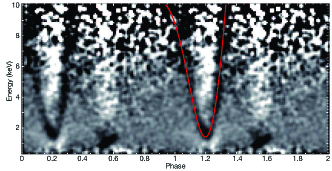
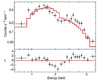
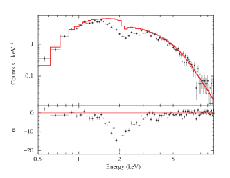
Figure 9: The top left figure shows an artist’s impression of the magnetic field topology inferred for the magnetar SGR 0418+5729 thanks to the discovery of a prominent cyclotron line around 2 keV [53]. The top right figure shows the cyclotron feature variation as a function of the magnetar spin-phase in a pulse-phase resolved spectrum as observed by XMM-Newton. The EPIC-pn spectrum corresponding to a specific phase interval (exposure time 613 s) is shown on the bottom left figure. The bottom right figure shows the simulated spectrum of the cyclotron feature observed in a specific 0.02-wide spin-phase interval and as would be detected in a 613-s long observation with eXTP SFA. It is evident that eXTP would have detected the same feature at a much larger significance in the same exposure time. In both cases, the cyclotron feature is not included in the model used to fit the data in order to highlight its presence in the residuals from the fits.

2.5 Magnetars in Binaries

Magnetars have been so far associated only with isolated sources. However, accreting magnetars in binary systems may exist. Based on our knowledge of the phenomenology of isolated magnetars, it has been proposed to search for accreting magnetars by looking for three signatures [58, 59]: (1) magnetar-like bursts in an accreting neutron star system; (2) a hard X-ray tail above $100\,\rm keV$; (3) an ultra-luminous X-ray pulsar (like that observed in M82, [60]). In fact, accreting magnetar systems may form a significant fraction of ultra-luminous X-ray sources [59, 61, 62].

With its large area, broad band and high sensitivity resolution, eXTP would be able to detect magnetars in binary systems in the future. Repeated magnetar-like bursts in an accreting system would be strong evidence for accreting magnetars and magnetism-powered activities [63]. Detecting such activity on top of the accretion powered flux requires, however, large effective area and long exposure times - provided for the first time by eXTP. The transition between the accretion phase and the propeller phase might also be used to uncover magnetars in binaries [58, 64], and detection of such a transition on short timescales also requires large effective area. Finally, the spin period evolution of X-ray pulsars monitored by WFM might also be used to find strongly magnetized objects.

3 Strong Magnetic Fields at work: accretion and rotation powered pulsars

3.1 Introduction

Emission from X-ray pulsars is powered by accretion of ionized gas onto strongly magnetized (B$\sim$10^12-13 G) rotating NSs. In this “magnetospheric” type of accretion, the plasma flow is disrupted by the rotating magnetosphere far away from the neutron star at the magnetospheric radius, $r_{\rm m}\sim 10^{9}$ cm, and funnelled along the field lines to the polar areas of the NS [65, 66]. Upon impact with the surface, the kinetic energy of the accretion flow is converted to X-ray emission, which appears to be pulsed due to the rotation of the NS.

The observational appearance of X-ray pulsars is diverse. It is defined by several factors including the nature and evolutionary status of the donor star, the parameters of the binary system, and of the neutron star [67, 66, 68]. In particular, the magnetic field strength and configuration define the geometry and physical conditions within the emission region and thus strongly affect the observed X-ray spectrum. On the other hand, the interaction of the accretion flow with the magnetosphere mediates the accretion rate, thus affecting detectability and variability properties of the pulsar, and this also defines the spin evolution of the neutron star.

A key probe of the magnetic field intensity is provided by the electron CRSFs observed in spectra of many X-ray pulsars. These line-like absorption features are associated with the resonant scattering of X-rays by plasma electrons in their Landau levels: $E^{(n)}\simeq(n+1){e\hbar B\over{m_{e}c}}$. The electron cyclotron energy depends only on the magnetic field in the line forming region $E_{cyc}=11.6(B/10^{12}\leavevmode\nobreak\ {\rm G})$ keV, so observations of the CRSFs provide a unique direct probe of the magnetic field in the line forming region. Given the typical NS fields of $\sim 10^{12}$ G, the CRSFs are observed at hard X-ray energies in X-ray pulsars (see [69, 70] and references therein).

The observed energy and shape of the CRSFs are, however, also affected by the geometrical configuration of the emission region and the orientation with respect to the observer. Indeed, given the strong angular dependence of the scattering cross-sections, observed spectra are expected to be significantly different when most of the photons are propagating predominantly along as opposed to predominantly across the magnetic field. For a rotating pulsar, this implies a strong dependence of the observed X-ray spectra on pulse phase, which can be used to probe the geometry and physical properties within the emission region.

Note that the geometry of the emission region can change with the accretion rate, so the spectra of X-ray pulsars also change with luminosity. It was proposed by [71] that a major change in the geometry of the emission region must occur close to the local Eddington luminosity $L_{E}$, at the so-called critical luminosity $L_{c}\sim 10^{37}$erg s^-1 [72, 74]. At low luminosities ($L<L_{c}$) the influence of the radiation on the infalling matter is negligible, so the kinetic energy of the accretion flow is only released upon the impact with the NS surface, forming hot compact polar caps. The opacity of strongly magnetized plasma is lower along the field lines, so the Comptonized X-rays escape predominantly upwards along the field, and form a so-called “pencil-beam” pattern. At higher luminosities ($L>L_{c}$), a radiation dominated shock rises above the neutron star surface, forming an extended accretion column [71, 76, 77]. In this case, the photons can only escape through the sidewalls of the column, and a “fan” emission pattern is predicted.

As already mentioned, the pulse phase dependence of X-ray spectra is expected to be drastically different for the two geometries, so pulse-phase resolved spectroscopy is commonly used to probe the accretion regime. Unfortunately, interpretation of the results is complicated by the fact that both poles of the neutron star might be visible at all pulse phases, and it is not trivial to disentangle their respective contribution. Analysis of pulse-phase resolved spectra in a range of luminosities can be used to reconstruct the intrinsic spectra and beam patterns of the two poles [85], which is an essential step in interpretation of the observed spectra. Such analysis requires, however, several additional assumptions and high quality observations, particularly below the critical luminosity. This implies low observed fluxes, and is thus challenging for existing facilities.

Scattering of the emerging X-rays in strongly magnetized plasma is also expected to induce a high degree of linear polarization of the observed emission. Polarisation properties are expected to depend strongly on the orientation with respect to the magnetic field, and to be sensitive to the emission region geometry. Polarimetric observations are thus highly complementary to the more traditional techniques, and can be used to reduce the number of assumptions required to reconstruct intrinsic beam patterns and spectra of X-ray pulsars. eXTP will be the first mission to provide simultaneously both X-ray polarimetry and large effective area essential for pulse-phase and luminosity resolved spectroscopy.

3.2 Pulse phase and luminosity resolved spectroscopy

In high luminosity sources most of the observed emission is expected to come from the accretion column with a “fan” beam pattern. The observed CRSF energy in this case depends on the height of the visible part of the accretion column. The magnetic field is weaker away from the NS surface, so the energy of the CRSF formed in the upper parts of the column is lower. Variations of the observed line energy with pulse phase are therefore believed to be associated with changes in visibility of different parts of the column, partially eclipsed by the neutron star.

The height of the column increases with luminosity, so a luminosity dependence of the CRSF energy is also expected. In particular, an anti-correlation of the observed line energy with flux is most often attributed to the increase of the accretion column height with luminosity. Alternatively, the line may form in the NS’s atmosphere illuminated by the accretion column. In this case the observed anti-correlation of CRSF energy with flux in super-critical sources can be attributed to a change of the illumination pattern associated with column height variations [78, 79]. In either case, this effect can be probed through analysis of the dependence of the observed line energy on luminosity, and used to constrain the physical properties of the accretion column.

On the other hand, a correlation of the CRSF energy with flux has been reported for low luminosity sources [82]. Here the observed change of the CRSF energy is also believed to be due to a change of the line forming region height, which is expected in this case to decrease with luminosity [82]. Alternatively, the observed correlation of the line energy with flux in low luminosity sources can be attributed to Doppler shifts due to variation of the accretion flow velocity [75].

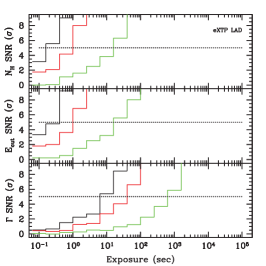
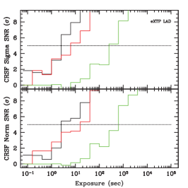
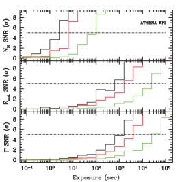
Figure 10: Left panel: an example of the eXTP LAD capability to reconstruct the spectral shape of an accreting X-ray pulsar in very short integration times. Simulations were performed using the results of a BeppoSAX observation of Vela X-1 [88]. Each curve gives the significance of a spectral parameter (defined as the ratio between the best fit parameter and its uncertainty) as a function of the exposure time. The curves are color coded according to the assumed flux (black: 500 mCrab, red: 150 mCrab, green: 15 mCrab). Middle panel: Same as before but showing the LAD capabilities in the case of 4U 0115+634. For this source, we show the significance of the CRSF detection at 12.8 keV using the spectral model proposed by [70]. “Norm” is the CRSF normalization and “Sigma” its width. We do not plot the significance of the CRSF centroid energy, as it is always determined at very high significance. The LAD can indeed measure the CRSF centroid energy at a significance level of 100, 20, and 3$\sigma$ for fluxes of 500, 150, and 15 mCrab, respectively in only 0.1 s. Right panel: Same as the left panel, but for Athena/WFI. This shows that similar studies are only possible if the LAD large collecting area is available. Other currently planned X-ray instruments would need overly long exposure times to achieve accurate spectral measurements.

The large effective area and superb energy resolution of eXTP LAD will allow us to monitor luminosity-related changes of the observed CRSF energy in transient sources, with unprecedented accuracy. As illustrated in Fig. 12 or the eXTP observatory science white paper, eXTP is capable of constraining line parameters with high accuracy across a wide range of luminosities, which will enable detection of the accretion regime transition in many sources sources.

In addition, eXTP will bring pulse phase and luminosity resolved spectroscopy to an entirely new level.v Pulse phase resolved analysis has so far been hampered by the fact that with existing facilities, one must average the source spectrum at a given phase over many individual pulses. This provides, however, information only on the averaged properties of the emission region, whereas the relevant timescale for intrinsic changes is comparable to or shorter than the spin period of the neutron star. Lack of information on spectral variations on short timescales thus limits the development of theoretical models [see, e.g., 81, for a recent review], as a result of which these topics remain highly debated [82, 83, 84, 72, 79].

The large throughput of the LAD will allow us, for the first time, to accurately constrain spectral properties of accreting X-ray pulsars, by using integration times much shorter than a single NS pulse. This is illustrated in Fig. 10 for two X-ray pulsars prototypes: Vela X-1 and 4U 0115+634. It is worth mentioning that given the optimal response and effective area of the LAD at 6-8 keV, pulse phase resolved spectroscopy will not be limited to CRSFs and broadband continuum, but will naturally encompass other spectral features, e.g., the fluorescence iron-K emission line (simulations show that the typical iron line observed in Vela X-1 can be constrained by the LAD with an integration time $\lesssim$10 sec).

The LAD will also be able to perform pulse phase spectroscopy at low luminosities, a regime not yet investigated due to the lack of simultaneous broad-band energy coverage, energy resolution, and collecting area of past and present X-ray facilities. Particularly intriguing is the variation of the cyclotron line energy with luminosity observed in several sources, see e.g., [86]. As already mentioned, such a variation most probably reflects a vertical displacement of the emitting region in the inhomogeneous magnetic field of the NS, and has to date been investigated mostly at luminosities $\gtrsim$10³⁷ erg s^-1 with relatively long pointed RXTE and INTEGRAL observations [see, e.g., 87, and references therein]. At luminosities below $\sim$10³⁷ erg s^-1 the accretion column is expected to disappear, so a different dependence of the cyclotron line energy $E_{\rm cyc}$ on flux [72] might be anticipated. Such a transition has indeed been recently observed in a bright transient V 0332+53 [73] with NuSTAR. However, observations with eXTP/LAD will allow us not only to obtain similar results for a larger number of sources, but also to investigate for the first time the pulse-phase dependence of the spectrum at low luminosities. Simulations in Fig. 10 show that the LAD will be able to measure spectral parameters of the CRSF of accreting pulsars at high significance ($\gtrsim 5\sigma$) in less than several hundreds of seconds, even at luminosities as low as a few tens of mCrab.

3.3 Polarisation studies of accreting pulsars

Photon scattering in magnetized plasma is also expected to lead to strong polarization of the emerging X-rays. In strong magnetic fields the radiation propagates in two, linearly polarized modes: the ordinary O- and the extraordinary X-mode, which are parallel and perpendicular, respectively, to the B-field. The difference in opacities for the ordinary and extraordinary modes implies strong birefringence for propagating photons and thus strong polarization of the emerging radiation. In their seminal paper, [80] showed that the X-ray linear polarization depends strongly on the geometry of the emission region, and varies with energy and pulse phase, reaching very high degrees, up to 70%, for favorable orientations [80]. The accreting pulsars are also among the brightest X-ray sources in the sky and are thus a prime target for X-ray polarimetric observations.

For photons propagating along the field (“pencil beam”) the weakest polarization is expected when the flux amplitude is at its maximum. On the other hand, for “fan beam” the amplitude of polarization is maximum when the flux amplitude is maximum. The phase swing (from positive to negative and viceversa) of the polarization angle with respect to the flux maxima and minima also clearly depends on the beaming geometry (“fan” vs. “pencil”). Phase resolved measurements of the linear polarization thus constitute a decisive test to distinguish between the two scenarios. In other words, phase-resolved polarimetry can help to constrain the radiation pattern model and also the value of the viewing geometry (e.g. the angle that the observer line-of-sight makes with the pulsar magnetic axis) as functions of the rotational phase. In addition, since the components forming the overall beam pattern may dominate at different energies, the energy dependence of the degree and angle of polarization can be observed. This information can be used to disentangle unambiguously the contributions of the two NS poles and thus contribute solving the long-standing problem of radiation formation in accreting pulsars. For instance, polarization measurements will immediately test the reflection model for the CRSF formation suggested by [79]. We also observe that the phase swing of polarization angle can be used to infer the angle between the rotation and the magnetic dipole axes, a free parameter of the state of the art models for pulse profile formation.

Assuming the simple scenarios predicted by [80], we show in Fig. 11 a simulation for the PFA onboard eXTP of the bright accreting pulsar Vela X-1, for the two cases of pencil and fan beam. Phase resolved linear polarization degree and angle are shown for ten phase bins with 7 ks/phase bin exposure, i.e. for a modest total exposure of 70 ks. In the specific example shown here, it is $i_{1}=45^{\circ}$ and $i_{2}=45^{\circ}$, where the angle $i_{1}$ refers to the angle between the spin axis and the line of sight, while $i_{2}$ corresponds to the angle beween the spin and the magnetic field axes (see [80] for more detail on the assumed emission region geometry). The two cases will be neatly distinguished with the eXTP PFA. As expected, the polarization fraction is maximum at the pulse peak for the fan beam pattern, and minimal for a pencil beam. The skewed dependence of the polarization angle in the two cases is due to the assumed geometry (i.e. magnetic/spin inclination), which it can be used to constrain. The beam pattern emerging from the NS is certainly more complex, and will most likely be a combination of simpler beam geometries. This will lead to a more complex phase-dependence of the fraction and angle of polarization. Moreover, since different beam patterns are expected to be dominant at different energies, we may observe phase resolved profiles of linear polarization fraction and angle which changes with energy. The measurements of the viewing angles $i_{1}$ and $i_{2}$, which will allow us to constrain the geometry of the system, requires a more careful modelling of the emission region. Several modelling efforts aiming to assess accurately the expected phase and energy dependence of the polarization properties and flux have been already started.

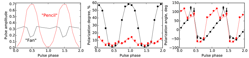
Figure 11: The pulse amplitude, the linear polarization fraction and the degree of polarization as a function of the pulse phase are shown, assuming the spectrum of Vela X-1. An exposure of 7 ks/phase has been chosen together with 10 phases. Total exposure is 70 ks. A combination of $i_{1}=45\circ$ and $i_{2}=45\circ$ has also been chosen.

X-ray pulsars are among the brightest sources in the sky and are expected to be strongly polarized, so the characterization of the polarization properties of most persistent sources and transients in outburst is within reach of eXTP measurements. This includes both comparatively dim nearby sources and bright transients throughout the Milky Way. In the case of bright persistent sources, exposures of the order of $\sim 10$ ks will be sufficient for the detailed studies, while significant polarization will be detected in weak sources within $\sim 100$ ks, which still allows phase resolved studies on the Ms timescale. In fact, for several objects the PFA will be sensitive enough to study polarization in both sub- and super-critical accretion regimes as illustrated in Fig. 12 of the eXTP observatory science paper. Such observations would be particularly important, as the transition from super- to sub-critical accretion is expected to completely change the beam pattern and the polarization properties of the pulsar, and thus they represent an ultimate test for the theoretical models.

3.4 Inside the NS magnetosphere: microsecond variability in High Mass X-ray Binaries (HMXBs)

In wind-accreting NSs, the plasma is thought to penetrate the magnetosphere through Rayleigh-Taylor instabilities, in the form of accreting blobs [89, 90]. These blobs, after a short radial infall, are channeled by the magnetic field lines onto the NS polar caps, where they release their kinetic energy as X-ray radiation. A sort of “granularity” is thus expected in the observed X-ray emission [91], and the energy release of each shot occurs on microsecond timescales [92]. The transport of the microsecond pulses through the NS magnetosphere will tend to broaden them, but photons at energies lower than the cyclotron energy, moving in a direction parallel to that of the magnetic field, would emerge unscattered because scattering is drastically reduced [93]. Since the typical cyclotron resonance energies observed in accreting X-ray pulsars are $E\lesssim 5$ keV, it is expected that $\mu$s pulses from the surface of NSs should be detectable relatively undistorted.

To detect such $\mu$s variability, we plan to use multiple detector coincidence. The LAD is therefore the best suited instrument for this kind of studies, given its time resolution and the high number of independent detection modules, $N_{d}$. The presence of events at $\mu$s time scales can be probed by building a time interval histogram with 5 $\mu$s resolution. By performing multiple detector coincidence, it is possible to discriminate between events that occur within $5\;\mu$s in different detectors. If the X-rays arrive uncorrelated and at a constant rate, the resulting histogram follows an exponential decay. Any deviation from that will indicate coherence or correlation among the events. In particular, microsecond X-ray bursts could be identified as excesses in the time interval histogram. Following [92], we computed in Fig. 12 the rate $R_{B}$ of true bursts from coincidence timing among independent detectors, and the rate $R_{A}$ of accidental counts within $5\;\mu$s (e.g., coming from background fluctuations) for a LAD observation of Vela X-1 in the low and high emission state [88].

According to the results of the simulation, the number of detected events (bursts plus accidentals) would be significantly greater than that of accidental events, even for a relatively small granularity of 10% in both the low and high emission states. For example, for the low state, the rate of multiple coincidence detection of true $\mu$s bursts is $R_{B}$=6..3 c/s, to be compared to the expected rate of observing accidental coincidences $R_{A}$=0.77 c/s [note that this is the rate of true bursts from multiple detector coincidence, not to be confused with the rate of formation of the blobs at the magnetospheric limit, $\lambda$, which is in the range 10-100 blobs/s; it is the squashing of these blobs that gives rise to the $\mu$s variability, as detailed in 91]. It is important to note that the signal to noise ratio (SNR) for the detection of microsecond variability scales with the square root of $\binom{N_{d}}{2}$. The RXTE PCA had $N_{d}=5$, therefore the number of pairs of detection modules with which to perform coincidence was $\binom{N_{d}}{2}=10$. For the LAD, $N_{d}$=41, and thus the S/N improvement over the PCA is $\gtrsim$30. No other flown or planned X-ray instrument is thus capable of performing such studies efficiently, apart from the LAD.

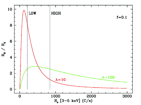
Figure 12: The unique capabilities of eXTP in detecting microsecond bursting activity from wind-accreting NSs. The ratio between the detection rate $R_{B}$ of true micro-bursts, and the rate $R_{A}$ of spurious bursts, is plotted as a function of the source count rate $R_{s}$, for the case of a moderate granularity (10%) in the accretion stream. The two vertical lines mark the count rates for two Vela X-1 luminosity states (low: 15 mCrab, soft spectrum; high: 45 mCrab, hard spectrum). $\lambda$ is the rate of formation of the blobs at the magnetospheric limit [91]. This would correspond to the number of rain drops formed in the handrail per unit time. $f$ is the granularity component in the accretion flow, here assumed to be 10%.

Variability on similar timescales is also expected in HMXBs due to so-called “photon bubble oscillations”. The latter were found to develop below the radiation dominated shock that terminates the free-fall motion of the accreting matter, in the accretion column of X-ray pulsars with luminosities $\gtrsim$10³⁷ erg s^-1 [94]. If convincingly detected, photon bubble oscillations can provide insights into the structure of the accretion column near the NS surface, and potentially an independent measurement of the compact object magnetic field [94]. Some evidence for the presence of variability induced by photon bubble oscillations was found in the HMXB Cen X-3, as two QPOs at 330 and 760 Hz have been reported in its power spectrum [94]. Such features could not be convincingly confirmed with the 5 PCUs of the RXTE PCA as dead time effects lowered the counting noise level of the instrument below the value expected for Poisson statistics, and a counting noise model needed to be included in the fit to the power spectra. In this case, the large number of detectors in the LAD again provides a unique advantage.

3.5 Rotation powered pulsars

According to the magnetic dipole model, the fast rotation ($\sim 1$ ms-$10$ s periods) of pulsars powers the acceleration of particles in the magnetosphere and the emission of electromagnetic radiation beamed around the magnetic axis, producing the characteristic pulsed emission if the magnetic and rotation axis are misaligned. For this reason they are also referred to as rotation-powered pulsars (RPPs), to be distinguished from other classes of isolated neutron stars, such as the magnetars, which are powered by their magnetic energy [95].

Thanks to its features, the LAD on board eXTP will make it possible to exploit the diagnostic power of high X-ray time and spectral resolution to make progress in understanding the radiation emission processes in pulsar magnetospheres. It is not yet completely established whether the emission at different energies (gamma-rays, X-rays, optical, radio) originates from different populations of relativistic particles and different regions (and altitudes) of the neutron star magnetosphere, nor whether this is related to the occurrence of breaks in the multi-wavelength power-law (PL) spectra. The light curve morphologies at different energies are very diverse and encode information about the orientation of the different emission beams with respect to the neutron star spin axis. Thus, from their comparison one can map the location of different emission regions in the neutron star magnetosphere, hence determining the origin and width of the emission beams at different energies, tracking the particle energy and density distribution in the magnetosphere, and measuring the neutron star spin axis/magnetic field orientation. Such a precise characterisation of pulsar light curves in different energy ranges will be key to building self-consistent emission models of the neutron star magnetosphere [96].

Over 200 gamma-ray pulsars have been now identified by the Large Area Telescope (LAT) aboard the Fermi Gamma-ray Space Telescope [97, 98]. Thus, gamma-ray detections of RPPs outnumber those in any energy range other than radio, and provide us with a uniquely large and diverse sample to characterise pulsar light curves at different energies. Focussing, for instance, on the younger (age lower than $\sim 1$ Myr) and more energetic Fermi pulsars, fewer than 30 of them show pulsed X-ray emission, whereas another 40 or so also have (non pulsed) detections in the X-rays [99]. The LAD on the eXTP mission will accurately measure X-ray light curves and detect pulsations for Fermi pulsars more efficiently than any other previous mission. We simulated the sensitivity to the detection of X-ray pulsations at the gamma ray pulse period with the LAD in the 2-10 keV energy band assuming a single-peak X-ray light curve with a Lorentzian profile, variable pulsed fraction, and peak full width half maximum (FWHM). We assumed a power law X-ray spectrum with a photon index of $\Gamma=1.5$ and hydrogen column density $N_{H}$ fixed to the Galactic value along the line of sight. For instance, in the event of a 50% pulsed fraction and 0.1 FWHM, in 30 ks we can detect X-ray pulsations, compute the pulsed fraction (10% error), and the peak phase (0.02 error) for pulsars with unabsorbed X-ray flux as low as $3\times 10^{-13}$ erg cm^-2 s^-1 in 0.5-10 keV. In case of a sinusoidal profile, in 30 ks we can reach the same accuracy in the light curve characterisation for pulsars with an unabsorbed X-ray flux as low as $6\times 10^{-13}$ erg cm^-2 s^-1. This means that we can obtain X-ray light curves with the accuracy claimed above for at least 20 of the younger Fermi pulsars currently detected in the X-rays. Moreover, thanks to the LAD sensitivity up to 50 keV, we can increase by at least a factor of two the number of pulsars seen to pulsate in the hard X-rays.

Measurements of the X-ray polarization of RPPs, never performed to date but possible with the PFA on eXTP, will provide additional and unprecedented information on their highly-magnetized relativistic environments. For RPPs with X-ray flux as faint as $5\times 10^{-13}$ erg cm^-2 s^-1, we will be able to measure a minimum detectable X-ray polarization of 10% (time averaged) with an exposure time of 150 ks, and compare it with the expectations for the X-ray emission mechanisms (e.g., synchrotron). For the Crab pulsar ($4.4\times 10^{-9}$ erg cm^-2 s^-1), we will be able to measure the time-resolved polarization degree and polarization position angle with an integration time of 10 ks, and their variation as a function of the pulsar rotational phase, to be compared with predictions of pulsar magnetosphere models such as the outer gap, polar cap, and slot gap/caustic gap models, which predict different swing patterns of the polarization parameters.

Giant Radio Pulses (GRPs) occur in a handful of radio pulsars, mostly young RPPs. They can be defined as single pulse emission with an intensity that is significantly higher than the average. Early observations of GRPs indicated a possible correlation between GRP phenomena and the magnetic field strength at the light cylinder, whose radius is the distance of the last closed magnetic field line, possibly pointing to an outer magnetosphere origin. A correlation between Giant Pulses (GPs) in the radio and at higher energies has only been observed in the optical for the Crab pulsar ([100], [101],[102], where optical GPs show a $\sim$3% increase relative to the average peak flux intensity.

GPs have not yet been detected in the high-energy domain, with only upper limits on the relative peak flux increase obtained at soft ($<$200%; [103]) and hard X rays ($<$80%;[104]), soft ($<$250%; [105], high ([106]; $<$400%) and very high-energy gamma rays ($<$1000%; [107]).

From optical observations it appears that the observed energy excess in a GP is roughly the same in radio as in optical. If we scale from the optical to X-rays we consequently expect to see a similar flux increase. Our assumption is consistent with the first constraint on a GP strength in the Crab pulsar in the 15–75 keV energy range recently obtained with Suzaku in coincidence with a GRP ([108]).

The high count rate from the Crab pulsar with the LAD and its $1\,\mu$s absolute timing accuracy will allow studies of individual pulses. Thus it will be possible to detect, for the first time, GPs in X-rays from the Crab and in other relatively bright X-ray pulsars, monitor their correlation with GPs observed simultaneously in radio with the SKA and determine the correlation between coherent and incoherent radiation production mechanisms in the neutron star magnetosphere. According to our simulations (see [109] for details) we should be able to detect a 3% peak flux increase.

4 QED

4.1 Introduction

One of the first predictions of quantum electrodynamics, even before it was properly formulated, was vacuum birefringence [110, 111]; in particular that a strong magnetic field would affect the propagation of light through it. Even when QED was formulated more carefully over the following two decades [112], this prediction remained robust. In a weak magnetic field, the difference in the index of refraction between photons polarized in the O-mode and in the X-mode is simply [113]

$$\Delta n=\frac{\alpha}{4\pi}\frac{2}{15}\left(\frac{B}{4.4\times 10^{13}\leavevmode\nobreak\ \mathrm{G}}\right)^{2}.$$

For terrestrial fields, this is vanishingly small and has not yet been measured in the eighty years since the prediction. On the other hand, astrophysically this effect can be important for neutron stars, black holes and white dwarfs [114, 116]. For these objects, although the difference in index of refraction is still much smaller than unity, the combination $\Delta n(l/\lambda)$, where $l$ is the length over which the index of refraction changes and $\lambda$ is the wavelength of the light, may be very large. This means that the polarization states of the light evolve adiabatically, so light originally polarized in the X-mode will remain in the X-mode even if the direction of the field changes. From the point of view of the observer, the direction of the polarization will follow the direction of the magnetic field as the light propagates through it.

The crucial connection to eXTP is that magnetized neutron stars and accreting magnetized white dwarfs (polars) naturally produce polarized X-ray radiation, and furthermore the field strengths are sufficiently strong and the length scales sufficiently large that vacuum birefringence decouples the polarization modes, which can have a dramatic effect on the observed polarization. Although black holes themselves do not harbor magnetic fields, recent calculations also indicate that the vacuum polarization is important for the propagation of radiation near black hole accretion disks if magnetic fields provide the bulk of the viscosity [116]. Our first focus will be neutron stars.

4.2 Neutron Stars

Vacuum birefringence is strongest for magnetars, whose fields range from $10^{14}$ to $10^{15}$ G. It is for these objects that available calculations are the most comprehensive. Vacuum birefringence increases the expected linear polarization of the X-ray radiation from the surface of a neutron star from about 5-10% to nearly 100% [117]. It is nearly as strong for neutron stars with more typical magnetic fields of $10^{12}$ G. Fig. 13 depicts the results for a typical magnetic field and for a magnetar. For a magnetar, at the high photon energies observed by eXTP, the effect essentially saturates: without QED, the observed polarization is small, at most 20%, and depends on the radius of the star, while with QED the polarization is nearly 100%. For a more weakly magnetized star, the polarization fraction from the entire surface is also much higher than without QED but, tantalizingly, it is not saturated and depends on the radius of the neutron star.

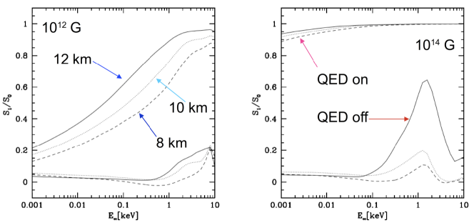
Figure 13: The expected fraction of linear polarization from the surface of strongly magnetized neutron stars with hydrogen atmospheres and effective temperatures of $10^{6.5}$ K. (from [117].

Depending on the particular source, the emission from thermal magnetars typically peaks around 2-3 keV, where the eXTP PFA will have an effective area of about 900 cm², with the gas-pixel detector (GPD) for polarization sensitivity. The 100% polarized radiation from the magnetar will result in about 40% modulation in the detector.

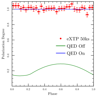
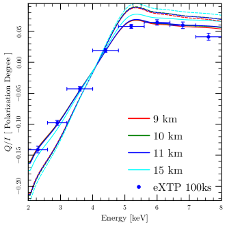
Figure 14: Left: The total degree of polarization as a function of phase expected from AXP 4U 0142+614 with and without QED averaged over energy. Right: Total polarization averaged over the rotation of Her X$-$1 (see text). The eXTP simulation assumes a radius of 10 km and QED. The solid curves include QED birefringence and the dashed curves do not.

Using the AXP 4U 0142+614 as an auspicious example, because its thermal emission is strong, we would expect to detect about 0.5 photons per second with energies between 2 and 4 keV with the PFA. The left panel of Fig. 14 depicts the energy-averaged polarized fraction expected from AXP 4U 0142$+$614 and the results of a 50 ks simulated observation with eXTP, as calculated in a simple model in which the whole NS surface is emitting at a homogeneous temperature. As it can be seen, this shows that the QED-off hypothesis can be rejected with a very high significance.

Recently, an optical polarimetry observation of an X-ray dim isolated neutron star (XDINS), RX J1856.5$−$3754 (with the magnetic field of $\sim 10^{13}$ G), performed with the VLT, showed a phase-averaged polarization fraction, PF$\sim$16%, consistent with the first ever evidence for QED vacuum birefringence induced by a strong magnetic field [118]. This important result can be confirmed by performing systematic polarimetry observations in the X-ray band, and the most promising sources are the brighest magnetars, either persistent or transient magnetars (hereafter TMs).

We have modeled the polarization properties of TMs in order to study the phase-averaged polarization fraction (PF) and polarization angle (PA) during the TM flux decay, adapting the method used by [119]. Based on the observational studies of representative sources such as XTE J1810$−$197 and CXOU J164710.2$−$455216 [120], we considered a TM with one hot polar cap, located at one of the magnetic poles, covering 15% of the star’s surface. We assume that, at the flux peak, the magnetosphere has a twist angle $\Delta\Phi=1.0$ rad and the hot polar cap has a uniform temperature of $T=1$ keV. When quiescence is reached, the magnetosphere has untwisted by $\Delta\Phi=0.5$ rad and the polar cap cooled down to $T=0.5$ keV. These values are reminiscent of those inferred by [120], when analyzing the outburst decay of XTE J1810$−$197 and CXOU J164710.2−455216. Once again, simulations (see [15, 16] for all details) show that the super-strong magnetic field surrounding TM can boost the observed PF of the thermal radiation, via the effect of vacuum birefringence, up to $\sim 99$% (considering the most favourable viewing geometry $\chi\sim 90^{\circ}$ and $\xi\sim 0^{\circ}$, see Fig. 15). We also found that when vacuum birefringence is operating, the value of PA can change by up to 23 degrees during a magnetospheric untwisting of $\sim$0.5 rad (as typically expected from outburst onset until quiescence, Fig. 16), offering an interesting test for the magnetar model. If vacuum birefringence were not present and the polar cap shrinks during the TM flux decay, we found that the PF would increase from ∼ 65% up to ∼ 99% (Fig. 17). If instead vacuum birefringence is operating, the PF stays almost constant, independent of the cap size. This is an interesting result, since the detection of a nearly constant PF as the decay proceeds will provide further evidence for the presence of vacuum birefringence.

Simulations (based on parameters for XTE J1810$-$197 and CXO J164710.2$−$455216, see [121, 122]) show that in order to observe a PF$\sim$70% and variation of the PA$\sim$10 deg, at the onset of the outburst (with a maximum flux $\sim 10^{-11}$ erg cm^-2 s^-1), the observation time required by eXTP is $\sim 3$ ks and $\sim 20$ ks respectively. At the end of the X-ray flux decay, when the TM is in quiescence (minimum flux $\sim 5\times 10^{-13}$ erg cm^-2 s^-1), the observation time required to detect the same PF and PA by eXTP is $\sim 60$ ks and $\sim 380$ ks, respectively. Examples are reported in Fig. 18 for the PF.

Comparatively short exposures enabled by large effective area of the eXTP also make it the only instrument able to carry out systematic studies of QED effects in multiple sources. Indeed, eXTP will have in place a monitoring programme of TMs, and will therefore represent a revolutionary instrument, capable of testing QED effects in TMs systematically, with short observations, in at least 1-2 sources per year.

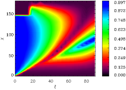
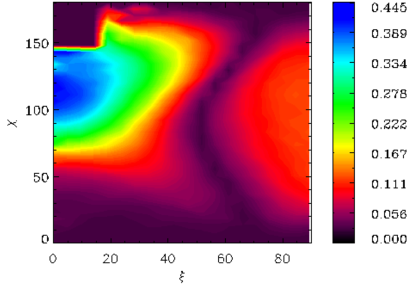
Figure 15: Left: phase-averaged PF for the thermal radiation emitted from a TM at the peak of the outburst (without vacuum birefringence) computed for different values of the angles $\xi$ (between the magnetic axis and spin axis) and $\chi$ (between the line of sight and spin axis). The radiation is computed for a magnetized NS atmosphere, with $B\sim 10^{14}$ G and assuming emission from one hot polar cap covering $15\%$ of the NS surface. Right: Same as in the left panel but accounting for the QED effects.

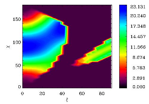
Figure 16: Expected variation of the phase-averaged PA for TMs during a magnetospheric untwisting of 0.5 rad (as expected during the outburst decay, for details see [15]), in the 2−6 keV energy range.

Fig. 19 depicts a second example where we can use magnetar observations to probe QED effects, and to verify the nature of the source, in particular the presence of a strong magnetic field in the emission region. The leading model for $\sim 1-10$ keV X-ray emission from magnetars is resonant inverse Compton scattering (RCS) of photons from the surface by charges carried in currents through the magnetosphere. In conjunction with the determination of the flux and flux variation, models of this emission also predict the change in the polarization of the high-energy magnetospheric emission with the spin of the neutron star, as calculated by [123]. Fig. 19 shows the simulated eXTP data for a bright persistent magnetar source with properties similar to those of the AXP 1RXS J170849.0-400910. Simulated data were obtained from the RCS model which best fits the 0.5-10 keV spectrum of the source, properly accounting for QED effects, and assuming a 100 ks exposure time. The mock data were then fitted with RCS models, either accounting for or disregarding QED effects. As expected, the pulse profile is well fitted in both cases (left panel), but the phase-dependence of the polarization fraction and angle (middle and right panels) are recovered only by QED-on models (middle and right panels). It is clear that, depending on how well the underlying model can be constrained by other observations, the QED-off case may be excluded to a large degree of confidence by such an observation with eXTP.

Figure 17: Maximum phase-averaged PF for different sizes of the polar cap (semi-angle of the polar cap). The line with asterisk symbols (*) corresponds to the case in which vacuum birefringence is operating. The line with crosses symbols (+) shows the case in which vacuum birefringence is not present. The radiation at the star surface is computed for a magnetized, pure-H atmosphere with $B_{p}=10^{14}$ G and temperature $T=0.5$ keV.

Figure 18: Simulations with eXTP showing the significance of a detection of a PF$\sim$70% (sufficient to prove QED effects) as a function of the exposure. Left: X-ray flux $\sim 10^{-11}$ erg cm^-2 s^-1, as typical of the outburst onset; Right: flux $\sim 5\times 10^{-13}$ erg cm^-2 s^-1, as representative of the quiescent state after decay.

Assuming discovery of the QED effect with eXTP, there are two natural directions in which to proceed. One is to use the QED effect to probe the other physical processes occurring in the source. The second is to measure the strength of the QED effect, effectively measuring the index of refraction of the magnetized vacuum. The left panel of Fig. 13 demonstrate this first avenue. In Fig. 13, we see how measurements of the polarized fraction of the surface emission at photon energies of few keV could provide an estimate of the radius of the neutron star (or more precisely $R_{\infty}=R[1-2GM/(c^{2}R)]^{-1/2}$). Although the figure shows the surface field, the strength of the QED effect depends on the strength of the dipole moment of the neutron star, which can be estimated, in principle, from its spin down, independent of the assumed radius of the star. For this to work, we would have to observe a more weakly magnetized neutron star that still exhibits thermal emission from the surface up to a few keV, where eXTP is sensitive, yet not so weak that one does not expect the thermal emission to be polarized at the surface (i.e. accreting millisecond pulsars would probably not work, but accreting X-ray pulsars might; however, in this case it might be difficult to obtain a reliable estimate of the magnetic field strength, if CRSFs are not observed).

The right panel of Fig. 14 depicts the polarized fraction as function of energy averaged over phase for the accreting X-ray pulsar Her X-1. We use the observed cyclotron resonance to constrain the magnetic field near the surface of the star and we use the spectral models of [80] and [115]. Because the emission comes from only a small fraction of the surface of the star, the effect of QED birefringence is to reduce the observed polarized fraction. Furthermore, the effect of QED is not saturated in this case, so with modeling one can determine the strength of the birefringence and possibly constrain the radius of the star as well.

Figure 19: Light curve, degree and angle of polarization as computed according to the “twisted magnetosphere” model with $\Delta\phi_{N-S}=0.5$ rad, $\beta=0.34$, $\chi=90^{\circ}$ and $\xi=60^{\circ}$ for a source with properties similar to those of the AXP 1RXS J170849.0-400910. Data points (filled circles with error bars) are generated assuming a 100 ks observation of the source and are drawn from the model shown by the blue dotted line; in both cases QED effects are fully taken into account (“ON” case). The red dotted line represents the same model but without vacuum birefringence (“OFF” case). The simultaneous fit (solid blue line) of the “ON” data with the “ON” model gives a reduced $\chi^{2}=1.14$ while that of “ON” data with the “OFF” model is ruled out with high confidence.

4.3 Black Holes and White Dwarfs

The theoretical treatment of the effects of vacuum polarization for black holes and white dwarfs is much less mature, but these objects also could provide exciting probes of QED, and vice versa. Black hole accretion disks are expected to generate a magnetic field much weaker than that of neutron stars, so one might think that the effect of vacuum birefringence on X-ray polarization would be small. However, how strongly the birefringence affects the polarization of the photon traveling in the magnetized vacuum depends not only on the strength of the magnetic field itself, but also on how long the photon travels in the strong magnetic field. Preliminary calculations [116] indicate that the vacuum polarization becomes important around $5-10$ keV, right in the middle of the eXTP sensitivity band.

[116] analyzed the effect of a chaotic magnetic field in the disk plane, for nearly edge-on observations of the disk. The chaotic field, in tandem with QED birefringence, depolarizes the radiation, as shown in Fig. 20. [116] performed Monte-Carlo simulations of 6,000 photons emitted with the same energy and angular momentum from the innermost stable circular orbit (ISCO) of the accretion disk of a rotating black hole, calculating the evolution of the polarization as each photon travels through the magnetosphere. The same simulation was performed for three different angular momenta of the photon (zero, maximum retrograde and maximum prograde), for ten different energies (from 1 to 10 keV), and for three different spins of the black hole ($a_{\star}=a/M=J/cM^{2}=0.5$, 0,7 and 0.9). The results are shown in Fig. 20. As we can see from the left panel, the QED effect can change the observed polarization, especially for red-shifted photons at the high end of eXTP’s energy range, where the observed polarization can be reduced up to 60% for a black hole rotating at 90% the critical velocity. The effect is larger for rapidly rotating black holes, for which red-shifted photons perform many rotations around the hole before leaving the magnetosphere (see the right panel of Fig. 20). These results are independent of the mass of the black hole.

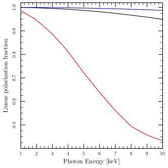
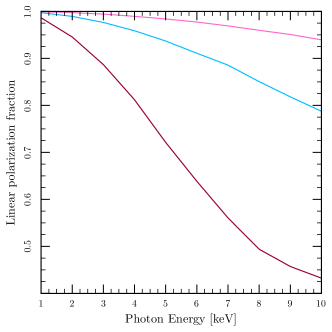
Figure 20: Observed polarization fraction against photon energy for an initial polarization fraction of one. Left: Zero angular momentum photons (black solid line), maximum prograde angular momentum photons (highly blue-shifted, blue solid line) and maximum retrograde angular momentum photons (highly red-shifted, red solid line), coming from the ISCO of a black hole with $a_{\star}=0.9$. Right: Maximum retrograde angular momentum photons for $a_{\star}=0.5$ (pink line), 0.7 (light blue line) and 0.9 (dark crimson line).

This analysis shows that QED must be taken into account when modeling the X-ray polarization from both stellar-mass and supermassive black hole accretion disks. In particular, it will be crucial in the understanding of QPOs, in which much of the variability in the flux results from our receiving alternately red-shifted and blue-shifted photons at the telescope. All the results in [116] are obtained for the minimum magnetic field needed for accretion to operate in the disk. A larger magnetic field would cause a higher depolarization at all energies. The observation of the X-ray polarization from black hole accretion disks would be, if properly modeled including QED, the first probe of black hole magnetic fields and the first direct way to study the role of magnetic fields in astrophysical accretion generally.

The potential of magnetized accreting white dwarfs for polarization measurements in the X-rays is tantalizing but completely unexplored. [114] argued that the polarized radiation should travel adiabatically near magnetized white dwarfs. These magnetized systems are, of course, known as polars because of the strong circular and linear polarization that they exhibit in the optical. These optical observations, where it is likely that plasma effects dominate, can give crucial information on the strength and geometry of the magnetic field near the white dwarfs. Furthermore, basic quantities like the radius of the white dwarf are well constrained theoretically and observationally. With these data in hand, these objects become ideal laboratories to probe QED, and in particular the more weakly magnetized white dwarfs (the intermediate polars or DQ Her stars) may offer the possibility of measuring the index of refraction through observations of polarized X-ray emission.

Acknowledgements. This paper is an initiative of the eXTP’s Science Working Group on Strong Magnetism, whose members are representatives of the astronomical community at large with a scientific interest in pursuing the successful implementation of eXTP. The paper was primaly written by by Andrea Santangelo, Silvia Zane, Hua Feng and Renxin Xu. Major contributions by Andrea Santangelo, Victor Doroshenko, Mauro Orlandini (3.1-3.4); Renxin Xu, Zhaosheng Li, Lin Lin (2.2., 2.3); Hao Tong (2.5); Silvia Zane (2.1, 2.2, 2.3.4, 2.4, 3.5, 4.1. 4.2); Nanda Rea, Paolo Esposito and Francesco Coti Zelati (2.2.2); Gianluca Israel and Daniela Huppenkoten (2.3.4); Roberto Turolla and Roberto Taverna (2.2.2., 4.2); Denis González-Caniulef (4.2); Roberto Mignani (3.5); Jeremy Heyl and Ilaria Caiazzo (4). Contributions were edited by Andrea Santangelo, Silvia Zane and Victor Doroshenko. Other co-authors provided valuable inputs to refine the paper. Financial contribution from the agreement between the Italian Space Agency and the Istituto Nazionale di Astrofisica ASI-INAF n.2017-14-H.O is acknowledged. This work is also partially supported by the Bundesministerium für Wirtschaft und Technologie through the Deutsches Zentrum für Luft- und Raumfahrt e.V. (DLR) under the grant number FKZ 50 OO 1701. The authors declare that they have no conflict of interest.

References

- [1] S-N. Zhang et al., Science China Physics, Mechanics& Astronomy, this issue (eXTP White Paper on the Instrumentation and Mission)
- [2] V. M. Kaspi, “Grand unification of neutron stars”, Proceedings of the National Academy of Sciences 107, 16, 7147, (2010).
- [3] R. C. Duncan, and C. Thompson, ApJ, 392, L9, 1992.
- [4] C. Thompson, and R. C. Duncan, ApJ, 408, 194, 1993.
- [5] S. Mareghetti, Astron. Astrophys. Rev., 15, 225, 2008.
- [6] H. Tong, Sci. China Phys. Mech. Astron., 59, 5752, 2016.
- [7] P. Sturrock, A. Harding, and J. Daugherty, ApJ346, 950, 1989.
- [8] R. Turolla, S. Zane, A. L. Watts, Rep. Prog. Phys., 78, 116901, 2015.
- [9] R. Taverna, and R. Turolla, MNRAS, 469, 3610, 2017.
- [10] A. I. Ibrahim, J. H. Swank, and W. Parke, ApJ584, L17, 2003.
- [11] G. Israel, P. Romano, and V. Mangano, ApJ685, 1114, 2008.
- [12] N. Rea, and P. Esposito, in High-Energy Emission from Pulsars and their systems, Proceedings of the First Session of the Sant Cugat Forum on Astrophysics, edited by N. Rea and D. Torres, ASSP series, p. 247, Springer, 2011.
- [13] F. A. Harrison, W. W. Craig, F. E. Christensen, et al., ApJ770, 103, 2013.
- [14] R. Taverna, F. Muleri, R. Turolla, et al., MNRAS, 438, 1686, 2014.
- [15] C. D. Gonzalez, Proceedings of Physics of Neutron Stars, 2017, Conference Series JPCS, 2017
- [16] Gonzalez, C. D. et al, 2017b, in prep
- [17] R. Archibald, V. M. Kaspi, C.Y. Ng, et al., Nature, 497, 591, 2013.
- [18] C. M. Espinoza, D. Antonopoulou, B. W. Stappers, et al., MNRAS, 440, 2755, 2014
- [19] A. Watts, C. M. Espinoza, R. Xu, et al., Proceedings of Advancing Astrophysics with the Square Kilometre Array (AASKA14). 9-13 June, 2014. Giardini Naxos, Italy, id.43, 2015
- [20] Y. Huang, and J. Geng, ApJ782, L20, 2014.
- [21] H. Tong, ApJ784, 86, 2014.
- [22] R. Xu, D. Tao, and Y. Yang, MNRAS Letters 373, L85, 2006.
- [23] E. Zhou, J. Lu, H. Tong, R. Xu, MNRAS, 443, 2705, 2014.
- [24] C. Thompson, M. Lyutikov, S. Kulkarni, ApJ, 574, 332, 2002.
- [25] K. Makishima, T. Enoto, J. S. Hiraga, et al., Phys. Rev. Letters, 112, 171102, 2014.
- [26] A. Sedkranian, A&A, 587, L2, 2016
- [27] A. Sedkranian, X. G. Huang, M. Sinha, et al, Proceedings of “Compact Stars in the QCD phase diagram V”, 23-27 May 2016 GSSI and LNGS, LÁquila, Italy, Journal of Physics: Conf. Series 861 012025, 2017
- [28] R. Xu, Adv. Space Res., 40, 1453, 2007.
- [29] A. Lyne, C. , Adv. Space Res., 40, 1453, 2007.
- [30] G. Hobbs, A, Lyne, and M. Kramer, MNRAS, 402, 1027, 2010.
- [31] Z. W. Ou, H. Tong, F. F. Kou, G. Q. Ding, MNRAS, 457, 3922, 2016.
- [32] H. Tong, R. Xu, L. Song, G. Qiao, ApJ, 768, 144, 2016.
- [33] F. Pintore, F. Bernardini, S. Mereghetti, P. Esposito, R. Turolla, et al., MNRAS, 458, 2088, 2016.
- [34] G. Israel, et al., ApJ, 628, L531, 2005.
- [35] A. Watts, T. E. Strohmayer, ApJ, 637, L117, 2006
- [36] T. E. Strohmayer, and A. L. Watts ApJ, 653, 593, 2006.
- [37] T. E. Strohmayer, and A. L. Watts ApJ, 632, L111, 2005.
- [38] D. Huppenkothen, A. L. Watts, Uttley P., et al., ApJ, 768, 87, 2013.
- [39] D. Huppenkothen, C. D’Angelo, A. L. Watts, et al., ApJ, 787, 128, 2014a.
- [40] D. Huppenkothen, L. M. Heil, A. L. Watts, E. Göğüş, ApJ, 795, 114, 2014b.
- [41] L. Samuelsson, and N. Andersson, MNRAS, 374, 256, 2007.
- [42] A. L. Watts, and S. Reddy, MNRAS Letters, 379, L63, 2007.
- [43] Y. Levin, MNRAS, 377, 159, 2007.
- [44] M. van Hoven, and Y. Levin, MNRAS, 410, 1036, 2011.
- [45] M. van Hoven, and Y. Levin, MNRAS, 420, 3035, 2012.
- [46] A. Colaiuda, K. D. Kokkotas, MNRAS, 414, 3014, 2011.
- [47] M. Gabler, P. Cerdá-Durán, N. Stergioulas, J. A. Font, and E. Müller, MNRAS, 421, 2054, 2012.
- [48] M. Gabler, P. Cerdá-Durán, J. A. Font, E. Müller, and N. Stergioulas, MNRAS, 430, 1811, 2013.
- [49] N. Andersson, K. Glampedakis, and B. Haskell, Phys. Rev. D, 79, 103009, 2009.
- [50] A. W. Steiner, and A. L. Watts, Phys. Rev. Letters, 103, 181101, 2009.
- [51] A. Passamonti, and S. K. Lander, MNRAS, 429, 767, 2013.
- [52] A. Passamonti, and S. K. Lander, MNRAS, 438, 156, 2014.
- [53] A. Tiengo, P. Esposito, S. Merghetti, R. Turolla, L. Nobili, and F. Gastaldello, et al., Nature, 500, 312, 2013.
- [54] P. Esposito, G. L. Israel, R. Turolla, A. Tiengo, and D. Götz, MNRAS, 405, 1787, 2010.
- [55] G. A. Rodríguez Castillo, G. L. Israel, A. Tiengo, D. Salvetti, R. Turolla, et al., MNRAS, 456, 4145, 2016.
- [56] A. Borghese, N. Rea, F. Coti Zelati, A. Tiengo, and R. Turolla, ApJ, 807, L20, 2015.
- [57] A. Borghese, N. Rea, F. Coti Zelati, A. Tiengo, R. Turolla et al., MNRAS, 468, 2975, 2017.
- [58] H. Tong, Res. Astron. Astrophys., 15, 517, 2015.
- [59] S. S Tsygankov, A. A. Mushtukov, V. F. Suleimanov, J. Poutanen, MNRAS, 457, 1101, 2016.
- [60] D. F. Torres, N. Rea, P. Esposito, J. Li, Y. Chen, and S. Zhang, ApJ, 744, 106, 2012.
- [61] G. L. Israel, A. Papitto, P. Esposito, et al., MNRAS, 466, L48, 2017
- [62] G. L. Israel, A. Belfiore, L. Stella, et al., Science, 355, 817, 2017
- [63] M. Bachetti, F. A. Harrison, D. J. Walton, B. W. Grefenstette, D. Chakrabarti, et al., Nature, 514, 202, 2014.
- [64] S. Dall’Osso, R. Perna, and L. Stella, MNRAS, 449, 2144, 2015.
- [65] P. Ghosh, and F. K., ApJ232, 259, 1979.
- [66] V. Doroshenko, A. Santangelo, and V. Suleimano, A&A, 529, A52, 2011.
- [67] E. Bozzo, M. Falanga , and L. Stella, ApJ, 683, 1031, 2008.
- [68] V. Doroshenko, A. Santangelo, L. Ducci, and D. Klochkov, A&A, 548, A19, 2012.
- [69] M. Revnivtsev, and S. Mereghetti, Space Sci. Rev., 191, 293, 2015.
- [70] A. Santangelo, A. Segreto, S. Giarrusso, D. Dal Fiume, and M. Orlandini, A&A, 523, L85, 1975.
- [71] M. M Basko, and R. A. Sunyaev, MNRAS, 175, 395, 1976.
- [72] P. A. Becker, D. Klochkov, G. Schönherr, O. Nishimura, and C. Ferrigno, et al., A&A, 544, A123, 2012.
- [73] V. Doroshenko, S. Tsygankov, A. Mushtukov, A. Lutovinov, A. Santangelo, V. Suleimanov, J. Poutanen, 466, 2143, MNRAS, 2017.
- [74] A. A. Mushtukov, V. F. Suleimanov, S. S. Tsygankov, and J. Poutanen, MNRAS, 447, 1847, 2015.
- [75] A Mushtukov, S. Tsygankov, A. Serber, V. Suleimanov, J. Poutanen, MNRAS, 454, 2714, 2015.
- [76] D. J. Burnard, J. Arons, and R. I. Klein, ApJ, 367, 575, 1991.
- [77] P. A. Becker, and M. T. Wolff, ApJ, 654, 435, 2007.
- [78] C. Ferrigno, P. A. Becker, A. Segreto, T. Mineo, and A. Santangelo, A&A, 498, 825, 2009.
- [79] J. Poutanen, A. A. Mushtukov, V. F. Suleimanov, S. S. Tsygankov, and D. I. Nagirner, et al., A&A, 777, 115, 2013.
- [80] P. Meszaros, R. Novick, A. Szentgyorgyi, G. A. Chanan, and M. C. Weisskopf, ApJ, 324, 1056, 1988.
- [81] G. Schönherr, F. Schwarm, S. Falkner, P. Becker, and J. Wilms, in: Physics at the Magnetospheric Boundary, Geneva, Switzerland, June 25-28, 2013, edited by E. Bozzo, P. Kretschmar, M. Audard, M. Falanga and C. Ferrigno, European Physical Journal Web of Conferences, 64, 2003, 2014.
- [82] R. Staubert, N. I. Shakura, K. Postnov, J. Wilms, and R. E. Rothschild, et al., A&A, 465, L25, 2007.
- [83] G. Schönherr, J. Wilms, P. Kretschmar, I. Kreykenbohm, and A. Santangelo, et al., A&A, 472, 353, 2007.
- [84] O. Nishimura, ApJ, 730, 106, 2011.
- [85] U. Kraus, C. Zahn, C. Weth, H. Ruder, ApJ, 590, 424, 2003
- [86] D. Klochkov, C. Ferrigno, A. Santangelo, R. Staubert, and P. Kretschmar, et al., A&A 536, L8, 2011.
- [87] D. Klochkov, R. Staubert, A. Santangelo, R E. Rothschild, and C. Ferrigno, et al., A&A, 532, A126, 2011.
- [88] M. Orlandini, D. dal Fiume, F. Frontera, G. Cusumano, and S. del Sordo, A&A, 332, 121, 1998.
- [89] J. Arons, and S. M. Lea, ApJ, 210, 792, 1976.
- [90] N. Shakura, K. Postnov, A. Kochetkova, and L. Hjalmarsdotter, MNRAS, 420, 216, 2012.
- [91] M. Orlandini, and G. E. Morfill, ApJ, 386, 703, 1992.
- [92] M. Orlandini, and E. Boldt, ApJ, 419, 776, 1993.
- [93] H. Herold, Phys. Rev. D, 19, 2868, 1979.
- [94] R. I. Klein, J. Arons, G. Jernigan, and J. J.-L. Hsu, ApJ, 457, L85, 1996.
- [95] R. Turolla, S. Zane, and A. L. Watts, Reports on Progress in Physics, 78, 116901, 2015.
- [96] M. Pierbattista, A. K. Harding, P. L. Gonthier, and I. A. Grenier, A&A, 588, A137, 2016.
- [97] P. A. Caraveo, Annu. Rev. Astron. Astrophys., 52, 211, 2014.
- [98] I. A. Grenier, and A. K. Harding, Comptes Rendus Physique, 16, 587, 2015.
- [99] M. Marelli, R. P. Mignani, A. De Luca, P. M. Saz Parkinson, and D. Salvetti, ApJ, 802, 78, 2015.
- [100] Shearer, A., et al., Science, 301, 493, 2003
- [101] Collins, S., et al., New Horizons in Time-Domain Astronomy, Proceedings of the International Astronomical, Union, IAU Symposium 285, 296, 2012.
- [102] Strader, M. J., et al., ApJ, 779, L12, 2013.
- [103] A. V. Bilous, M. A. McLaughlin, V. I. Kondratiev, and S. M. Ransom, ApJ., 749, 24, 2012
- [104] Hitomi Collaboration, PASJ, accepted, arXiv:1707.08801, 2017
- [105] Lundgren, S. C., et al., ApJ, 453, 433, 1995.
- [106] Bilous, A.V., Kondratiev, V. I., McLaughlin, M. A., et al. ApJ, 728, 110, 2011.
- [107] Aliu, E., et al., ApJ., 760, 136, 2012.
- [108] Mikami, R., et al., Suzaku-MAXI 2014: Expanding the Frontiers of the X-ray Universe, p.180, 2014
- [109] Mignani et al. arXiv:1501.02773, LOFT white paper, 2015.
- [110] W. Heisenberg, and H. Euler, Z. Physik, 98, 714, 1936.
- [111] V. S. Weisskopf, Uber die elektrodynamik des vakuums auf grund der quantentheorie des elektrons, Kongelige Danske Videnskaberns Selskab, Mathematisk-Fysiske Meddelelser, 14, 1, 1936.
- [112] J. Schwinger, Phys. Rev., 82, 664, 1951.
- [113] J. S Heyl, L. Hernquist, Journal of Physics A, 30, 6485, 1997.
- [114] J. S Heyl, N. J Shaviv, MNRAS, 311, 555, 2000.
- [115] Kii, T., PASJ, 39, 781 1987.
- [116] I. Caiazzo and J. Heyl, PRD, 2017, submitted.
- [117] J. S. Heyl, D. Lloyd, N. J. Shaviv, The High-Energy Polarization-Limiting Radius of Neutron Star Magnetospheres II – Magnetized Hydrogen Atmospheres, ArXiv Astrophysics e-prints, astro-ph/0502351.
- [118] R. Mignani, V. Testa, D. Gonzalez Caniulef, R. Taverna et al. MNRAS, 465, 492, 2017
- [119] D. Gonzalez Caniulef, S. Zane, R. Taverna, R. Turolla and K. Wu, MNRAS, 459, 3585, 2016
- [120] A. Albano, R. Turolla, G. Israel, et al. ApJ, 722, 788, 2010
- [121] F. Bernardini, G. Israel, S. Dall’Osso, et al, A&A , 498, 195, 2009
- [122] H. An, V. Kaspi, R. Archibald and A. Cumming, ApJ, 763, 82, 2013
- [123] R. Taverna, F. Muleri, R. Turolla, P. Soffitta, S. Fabiani, L. Nobili, MNRAS, 438, 1686, 2014.