Nonlinear Explicit Stochastic Attitude Filter on SO(3)

Abstract

This work proposes a nonlinear stochastic filter evolved on the Special Orthogonal Group $\mathbb{SO}\left(3\right)$ as a solution to the attitude filtering problem. One of the most common potential functions for nonlinear deterministic attitude observers is studied and reformulated to address the noise attached to the attitude dynamics. The resultant estimator and correction factor demonstrate convergence properties and remarkable ability to attenuate the noise. The stochastic dynamics of the attitude problem are mapped from $\mathbb{SO}\left(3\right)$ to Rodriguez vector. The proposed stochastic filter evolved on $\mathbb{SO}\left(3\right)$ guarantees that errors in the Rodriguez vector and estimates steer very close to the neighborhood of the origin and that the errors are semi-globally uniformly ultimately bounded in mean square. Simulation results illustrate the robustness of the proposed filter in the presence of high uncertainties in measurements.

I Introduction

The orientation of a rigid-body is termed attitude, and attitude estimation is an essential subtask in robotics applications [1, 2]. Unfortunately, the attitude cannot be accurately measured, however, the available measurements from sensors attached to the body-frame and inertial-frame coupled with an attitude filter allow reasonably accurate estimation of the true attitude. The moving vehicles are normally equipped with low-cost inertial measurement units (IMUs) which are very sensitive to noise and bias components, complicating the attitude estimation [1, 2].

Historically, the attitude filtering problem has been addressed using Gaussian filters based mainly on the structure of the Kalman filter (KF) [2]. The family of attitude Gaussian filters includes KF [3], extended KF (EKF) [4], multiplicative EKF (MEKF) [5], and others. However, attitude Gaussian filters have proven to be inefficient if the vehicle is equipped with low quality sensors [1, 2]. Other filtering techniques such as Unscented KF (UKF) [6] and particle filters (PFs) [7] provide a more precise estimation even when the low-quality sensors are used. However, the computational cost of the above-mentioned filters is higher [2]. It should be remarked that the Gaussian filters in [3, 4, 5] as well as UKF [6] and PFs [7] are quaternion based which does not provide a unique representation of the attitude [8].

The deficiencies of Gaussian filters, UKF and PFs, in addition to the development of low-cost IMUs, motivated researchers to design nonlinear deterministic attitude filters, such as [1, 9, 10]. These filters have better tracking performance than Gaussian filters [1] and require less computational power when compared with UKF and PFs [2]. In addition, nonlinear deterministic attitude filters evolve directly on $\mathbb{SO}\left(3\right)$ which is nonsingular in parameterization and has a unique representation. The deterministic filters proposed in [1, 9, 10] can be easily fitted given two or more vectorial measurements and a rate gyroscope measurement, however, the selected potential functions in [1, 9, 10] were kept unchanged. The potential function in [1, 9, 10] fits nonlinear deterministic attitude filters on $\mathbb{SO}\left(3\right)$ assuming that the rate gyro measurements are corrupted only with constant bias and are noise free. However, the environment is noisy [11, 12] and the kinematics of the nonlinear attitude problem on $\mathbb{SO}\left(3\right)$ in its natural stochastic sense need to be considered.

The main challenge is that the attitude problem is 1) modeled on the Lie group of $\mathbb{SO}\left(3\right)$ which is nonlinear and 2) the attitude dynamics are a function of angular velocity measurements which are corrupted with noise components. Therefore, the randomness and uncertain behavior in attitude kinematics prompted the proposal of nonlinear stochastic attitude filter on $\mathbb{SO}\left(3\right)$ based on the selection of a new potential function. Hence, in the case where angular velocity measurements are contaminated with noise, the stochastic filter would be able to guarantee that, 1) the error is regulated to an arbitrarily small neighborhood of the equilibrium point in probability; and 2) the error is semi-globally uniformly ultimately bounded (SGUUB) in mean square.

The rest of the paper is organized as follows: Section II gives an overview of mathematical notation and preliminaries. The problem is formulated in stochastic sense in Section III. The nonlinear stochastic filter on $\mathbb{SO}\left(3\right)$ is proposed and the stability analysis is presented in Section IV. Section V demonstrates the numerical results. Finally, closing notes are provided in Section VI.

II Math Notation

In this paper, $\mathbb{R}^{n}$ is the real $n$-dimensional space while $\mathbb{R}^{n\times m}$ denotes the real $n\times m$ dimensional space. For $x\in\mathbb{R}^{n}$, the Euclidean norm is defined as $\left\|x\right\|=\sqrt{x^{\top}x}$, where ^⊤ is the transpose of a component. $\mathcal{C}^{n}$ denotes the set of functions with continuous $n$th partial derivatives. $\mathbb{P}\left\{\cdot\right\}$, $\mathbb{E}\left[\cdot\right]$, ${\rm exp}\left(\cdot\right)$, and ${\rm Tr}\left\{\cdot\right\}$ refer to probability, expected value, exponential, and trace of a component, respectively. $\lambda\left(\cdot\right)$ is the set of eigenvalues of the associated matrix while $\underline{\lambda}\left(\cdot\right)$ is the minimum singular value. $\mathbf{I}_{n}$ denotes identity with dimensions $n$-by-$n$, and $\underline{\mathbf{0}}_{n}\in\mathbb{R}^{n}$ is a zero column vector. $\mathbb{SO}\left(3\right)$ denotes the Special Orthogonal Group, and the attitude of a rigid-body is defined as a rotational matrix $R$:

$$\mathbb{SO}\left(3\right):=\left\{\left.R\in\mathbb{R}^{3\times 3}\right|R^{\top}R=\mathbf{I}_{3}\text{, }{\rm det}\left(R\right)=1\right\}$$

where ${\rm det\left(\cdot\right)}$ is the determinant of the associated matrix. The Lie-algebra of $\mathbb{SO}\left(3\right)$ is known as $\mathfrak{so}\left(3\right)$ and is given by

$$\mathfrak{so}\left(3\right):=\left\{\left.\mathcal{Y}\in\mathbb{R}^{3\times 3}\right|\mathcal{Y}^{\top}=-\mathcal{Y}\right\}$$

with $\mathcal{Y}$ being the space of skew-symmetric matrices. Define the map $\left[\cdot\right]_{\times}:\mathbb{R}^{3}\rightarrow\mathfrak{so}\left(3\right)$ such that

$$\mathcal{Y}=\left[y\right]_{\times}=\left[\begin{array}[]{ccc}0&-y_{3}&y_{2}\\ y_{3}&0&-y_{1}\\ -y_{2}&y_{1}&0\end{array}\right],\hskip 10.00002pty=\left[\begin{array}[]{c}y_{1}\\ y_{2}\\ y_{3}\end{array}\right]$$

For all $\psi,\beta\in\mathbb{R}^{3}$, we have $\left[\psi\right]_{\times}\beta=\psi\times\beta$ where $\times$ is the cross product between the two vectors. Let the vex operator be the inverse of $\left[\cdot\right]_{\times}$, denoted by $\mathbf{vex}:\mathfrak{so}\left(3\right)\rightarrow\mathbb{R}^{3}$ such that $\mathbf{vex}\left(\mathcal{B}\right)=\beta$ for all $\beta\in\mathbb{R}^{3}$ and $\mathcal{B}\in\mathfrak{so}\left(3\right)$. Let $\boldsymbol{\mathcal{P}}_{a}$ denote the anti-symmetric projection operator on the Lie-algebra $\mathfrak{so}\left(3\right)$, defined by $\boldsymbol{\mathcal{P}}_{a}:\mathbb{R}^{3\times 3}\rightarrow\mathfrak{so}\left(3\right)$ such that $\boldsymbol{\mathcal{P}}_{a}\left(\mathcal{A}\right)=\frac{1}{2}\left(\mathcal{A}-\mathcal{A}^{\top}\right)\in\mathfrak{so}\left(3\right)$ for all $\mathcal{A}\in\mathbb{R}^{3\times 3}$. The normalized Euclidean distance of a rotation matrix on $\mathbb{SO}\left(3\right)$ is given by the following equation

$$\left\|R\right\|_{I}:=\frac{1}{4}{\rm Tr}\left\{\mathbf{I}_{3}-R\right\}$$ (1)

where $\left\|R\right\|_{I}\in\left[0,1\right]$. The attitude of a rigid body can be constructed knowing angle of rotation $\alpha\in\mathbb{R}$ and axis parameterization $u\in\mathbb{R}^{3}$. The mapping of angle-axis parameterization to $\mathbb{SO}\left(3\right)$ is defined by $\mathcal{R}_{\alpha}:\mathbb{R}\times\mathbb{R}^{3}\rightarrow\mathbb{SO}\left(3\right)$ such that

$$\mathcal{R}_{\alpha}\left(\alpha,u\right) =\mathbf{I}_{3}+\sin\left(\alpha\right)\left[u\right]_{\times}+\left(1-\cos\left(\alpha\right)\right)\left[u\right]_{\times}^{2}$$ (2)

The attitude could be obtained knowing Rodriguez parameters vector $\rho\in\mathbb{R}^{3}$ and $\mathcal{R}_{\rho}:\mathbb{R}^{3}\rightarrow\mathbb{SO}\left(3\right)$ [13] is

$$\mathcal{R}_{\rho}\left(\rho\right)= \frac{1}{1+\left\|\rho\right\|^{2}}\left(\left(1-\left\|\rho\right\|^{2}\right)\mathbf{I}_{3}+2\rho\rho^{\top}+2\left[\rho\right]_{\times}\right)$$ (3)

with direct substitution of (3) in (1) for $\mathcal{R}_{\rho}=\mathcal{R}_{\rho}\left(\rho\right)$ one obtains

$$||R||_{I}=\frac{1}{4}{\rm Tr}\left\{\mathbf{I}_{3}-\mathcal{R}_{\rho}\right\}=\frac{||\rho||^{2}}{1+||\rho||^{2}}$$ (4)

Likewise, the anti-symmetric projection operator of attitude $R$ in (3) can be defined as

$$\boldsymbol{\mathcal{P}}_{a}\left(R\right)=\frac{1}{2}\left(\mathcal{R}_{\rho}-\mathcal{R}_{\rho}^{\top}\right)= 2\frac{1}{1+||\rho||^{2}}\left[\rho\right]_{\times}$$

and the vex operator of the above-mentioned result is

$$\Phi\left(R\right)=\mathbf{vex}\left(\boldsymbol{\mathcal{P}}_{a}\left(R\right)\right)=2\frac{\rho}{1+||\rho||^{2}}$$ (5)

where $\Phi\left(\cdot\right)$ is the composition mapping such that $\Phi:=\mathbf{vex}\circ\boldsymbol{\mathcal{P}}_{a}$. The following identities will be used in the subsequent derivations

$$\left[\psi\times\beta\right]_{\times} =\beta\psi^{\top}-\psi\beta^{\top},\quad\psi,\beta\in{\rm\mathbb{R}}^{3}$$ (6)

$$\left[R\beta\right]_{\times} =R\left[\beta\right]_{\times}R^{\top},\quad R\in\mathbb{SO}\left(3\right),\beta\in\mathbb{R}^{3}$$ (7)

$$\left[\beta\right]_{\times}^{2} =-\beta^{\top}\beta\mathbf{I}_{3}+\beta\beta^{\top},\quad\beta\in\mathbb{R}^{3}$$ (8)

$$B\left[\beta\right]_{\times}+ \left[\beta\right]_{\times}B={\rm Tr}\left\{B\right\}\left[\beta\right]_{\times}-\left[B\beta\right]_{\times},$$

$$\quad B=B^{\top}\in\mathbb{R}^{3\times 3},\beta\in\mathbb{R}^{3}$$ (9)

$${\rm Tr}\left\{B\left[\beta\right]_{\times}\right\} =0,\quad B=B^{\top}\in\mathbb{R}^{3\times 3},\beta\in\mathbb{R}^{3}$$ (10)

III Problem Formulation

The attitude can be extracted from $n$-known non-collinear inertial vectors measured in a coordinate system fixed to the rigid body. Consider that the superscripts $\mathcal{I}$ and $\mathcal{B}$ refer to the vectors associated with the inertial-frame and body-frame, respectively. Let ${\rm v}_{i}^{\mathcal{B}}\in\mathbb{R}^{3}$ be the $i$th measurement vector in the body-fixed frame for $i=1,2,\ldots,n$. the orientation of the object in the body-frame $\left\{\mathcal{B}\right\}$ relative to the inertial-frame $\left\{\mathcal{I}\right\}$ can be represented by the attitude matrix $R\in\left\{\mathcal{B}\right\}$ as illustrated in Figure 1.

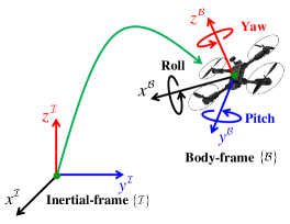
Figure 1: The relative orientation between body-frame and inertial-frame of a rigid-body in 3D space.

Let $R\in\mathbb{SO}\left(3\right)$ denote the rotation matrix from body-fixed frame to a given inertial-fixed frame such that the body-fixed frame vector is defined by

$${\rm v}_{i}^{\mathcal{B}}=R^{\top}{\rm v}_{i}^{\mathcal{I}}+b_{i}^{\mathcal{B}}+{\rm\omega}_{i}^{\mathcal{B}}$$ (11)

where ${\rm v}_{i}^{\mathcal{I}}\in\mathbb{R}^{3}$ denotes the inertial-fixed frame vector while $b_{i}^{\mathcal{B}}$ and ${\rm\omega}_{i}^{\mathcal{B}}$ denote the additive bias and noise components of the associated body-frame vector, respectively, for all $b_{i}^{\mathcal{B}},{\rm\omega}_{i}^{\mathcal{B}}\in\mathbb{R}^{3}$ and $i=1,2,\ldots,n$. The assumption that $n\geq 2$ is necessary for instantaneous three-dimensional attitude determination. It is common to employ the normalized values of reference and body-frame vectors in the process of attitude estimation such as

$$\upsilon_{i}^{\mathcal{I}}=\frac{{\rm v}_{i}^{\mathcal{I}}}{\left\|{\rm v}_{i}^{\mathcal{I}}\right\|},\hskip 10.00002pt\upsilon_{i}^{\mathcal{B}}=\frac{{\rm v}_{i}^{\mathcal{B}}}{\left\|{\rm v}_{i}^{\mathcal{B}}\right\|}$$ (12)

and the attitude can be defined knowing $\upsilon_{i}^{\mathcal{I}}$ and $\upsilon_{i}^{\mathcal{B}}$. For the sake of simplicity, the body frame vector (${\rm v}_{i}^{\mathcal{B}}$) is considered to be noise and bias free in the stability analysis. In the Simulation Section, on the contrary, noise and bias are present in the measurements. The true attitude dynamics and the associated Rodriguez vector dynamics are given in (13) and (14), respectively, as

$$\dot{R} =R\left[\Omega\right]_{\times}$$ (13)

$$\dot{\rho} =\frac{1}{2}\left(\mathbf{I}_{3}+\left[\rho\right]_{\times}+\rho\rho^{\top}\right)\Omega$$ (14)

where $\Omega\in\mathbb{R}^{3}$ denotes the true value of angular velocity. Gyroscope or the rate gyros measures the angular velocity vector in the body-frame relative to the inertial-frame. The measurement vector of angular velocity is

$$\Omega_{m}=\Omega+b+\omega$$ (15)

where $b$ and $\omega$ denote the additive bias and noise components, respectively, for all $b,\omega\in\mathbb{R}^{3}$. The noise vector $\omega$ is assumed to be a Gaussian noise vector such that $\mathbb{E}\left[\omega\right]=0$. The measurement of angular velocity vector is subject to additive noise and bias, which are characterized by randomness and unknown behavior, impairing the estimation process of the true attitude dynamics in (13) or (14). As such, (15) is assumed to be excited by a wide-band of random Gaussian noise process. Derivative of any Gaussian process yields a Gaussian process allowing the stochastic attitude dynamics to be written as a function of Brownian motion process vector [14, 15]

$$\omega=\mathcal{Q}\frac{d\beta}{dt}$$

where $\mathcal{Q}\in\mathbb{R}^{3\times 3}$ is a non-negative unknown time-variant diagonal matrix. In addition, each parameter of $\mathcal{Q}$ in the diagonal is bounded with an unknown bound. The properties of Brownian motion process can be found in [16, 17, 15]. The covariance component associated with noise $\omega$ can be defined by a diagonal matrix $\mathcal{Q}^{2}=\mathcal{Q}\mathcal{Q}^{\top}$. Considering the attitude dynamics in (14) and replacing $\omega$ by $\mathcal{Q}d\beta/dt$, the stochastic differential equation in (14) can be expressed by

$$d\rho= f\left(\rho,b\right)dt+g\left(\rho\right)\mathcal{Q}d\beta$$ (16)

Similarly, the stochastic dynamics of (13) are

$$dR=R\left[\Omega_{m}-b\right]_{\times}dt-R\left[\mathcal{Q}d\beta\right]_{\times}$$ (17)

where $g\left(\rho\right)=-\frac{1}{2}\left(\mathbf{I}_{3}+\left[\rho\right]_{\times}+\rho\rho^{\top}\right)$ and $f\left(\rho,b\right)=-g\left(\rho\right)\left(\Omega_{m}-b\right)$ with $g:\mathbb{R}^{3}\rightarrow\mathbb{R}^{3\times 3}$ and $f:\mathbb{R}^{3}\times\mathbb{R}^{3}\rightarrow\mathbb{R}^{3}$. $g$ is locally Lipschitz in $\rho$ and $f$ is locally Lipschitz in $\rho$ and $b$. Accordingly, the dynamic system in (16) has a solution on $t\in\left[t_{0},T\right]\forall t_{0}\leq T<\infty$ in the mean square sense for any $\rho\left(t\right)$ such that $t\neq t_{0}$, $\rho-\rho_{0}$ is independent of $\left\{\beta\left(\tau\right),\tau\geq t\right\},\forall t\in\left[t_{0},T\right]$ [17, 15]. Aiming to achieve adaptive stabilization of the unknown time-variant covariance matrix, let us introduce the following unknown constant

$$\sigma=\left[{\rm max}\left\{\mathcal{Q}_{1,1}^{2}\right\},{\rm max}\left\{\mathcal{Q}_{2,2}^{2}\right\},{\rm max}\left\{\mathcal{Q}_{3,3}^{2}\right\}\right]^{\top}$$ (18)

where ${\rm max}\left\{\cdot\right\}$ is the maximum value of the associated element. From (15), and (18), it can be noticed that $b$ and $\sigma$ are bounded. It is important to introduce the following Lemma which will be useful in the subsequent filter derivation.

Lemma 1.

Let $R\in\mathbb{SO}\left(3\right)$, $M^{\mathcal{I}}=\left(M^{\mathcal{I}}\right)^{\top}\in\mathbb{R}^{3\times 3}$, $M^{\mathcal{I}}$ be positive-definite, and ${\rm Tr}\left\{M^{\mathcal{I}}\right\}=3$. Define $\bar{\mathbf{M}}^{\mathcal{I}}={\rm Tr}\left\{M^{\mathcal{I}}\right\}\mathbf{I}_{3}-M^{\mathcal{I}}$ and let the minimum singular values of $\bar{\mathbf{M}}^{\mathcal{I}}$ be $\underline{\lambda}:=\underline{\lambda}\left(\bar{\mathbf{M}}^{\mathcal{I}}\right)$. Then, the following holds:

$$\left\|M^{\mathcal{I}}R\right\|_{I} =\frac{1}{2}\frac{\rho^{\top}\bar{\mathbf{M}}^{\mathcal{I}}\rho}{1+\left\|\rho\right\|^{2}}$$ (19)

$$\Phi\left(M^{\mathcal{I}}R\right) =\frac{\left(\mathbf{I}_{3}+\left[\rho\right]_{\times}\right)^{\top}\bar{\mathbf{M}}^{\mathcal{I}}}{1+\left\|\rho\right\|^{2}}\rho$$ (20)

$$\left\|M^{\mathcal{I}}R\right\|_{I} \leq\frac{2}{\underline{\lambda}}\frac{||\Phi\left(M^{\mathcal{I}}R\right)||^{2}}{1+{\rm Tr}\left\{\left(M^{\mathcal{I}}\right)^{-1}M^{\mathcal{I}}R\right\}}$$ (21)

Proof. See Appendix A.

Definition 1.

[18] The Rodriguez vector $\rho$ of the stochastic dynamics in (16) is known to be semi-globally uniformly ultimately bounded (SGUUB) if for a compact set $\Lambda\in\mathbb{R}^{3}$ and any $\rho_{0}=\rho\left(t_{0}\right)$, there exists a constant $\kappa>0$, and a time constant $T=T\left(\kappa,\rho_{0}\right)$ such that $\mathbb{E}\left[\left\|\rho\right\|\right]<\kappa,\forall t>t_{0}+T$.

Definition 2.

Consider the stochastic dynamics in (16). For a given function $V\left(\rho\right)\in\mathcal{C}^{2}$, the differential operator $\mathcal{L}V$ is defined by

$$\mathcal{L}V\left(\rho\right)=V_{\rho}^{\top}f\left(\rho,b\right)+\frac{1}{2}{\rm Tr}\left\{g\left(\rho\right)\mathcal{Q}^{2}g^{\top}\left(\rho\right)V_{\rho\rho}\right\}$$

such that $V_{\rho}=\partial V/\partial\rho$, and $V_{\rho\rho}=\partial^{2}V/\partial\rho^{2}$.

Lemma 2.

[17] Let the stochastic dynamics in (16) be given a potential function $V\in\mathcal{C}^{2}$ such that $V:\mathbb{R}^{3}\rightarrow\mathbb{R}^{+}$, class $\mathcal{K}_{\infty}$ functions $\varphi_{1}\left(\cdot\right)$ and $\varphi_{2}\left(\cdot\right)$, constants $c_{1}>0$ and $c_{2}\geq 0$, and a non-negative function $\boldsymbol{Z}\left(\left\|\rho\right\|\right)$ such that

$$\varphi_{1}\left(\left\|\rho\right\|\right)\leq V\left(\rho\right)\leq\varphi_{2}\left(\left\|\rho\right\|\right)$$ (22)

$$\mathcal{L}V\left(\rho\right)= V_{\rho}^{\top}f\left(\rho,b\right)+\frac{1}{2}{\rm Tr}\left\{g\left(\rho\right)\mathcal{Q}^{2}g^{\top}\left(\rho\right)V_{\rho\rho}\right\}$$

$$\leq -c_{1}\boldsymbol{Z}\left(\left\|\rho\right\|\right)+c_{2}$$ (23)

then for $\rho_{0}\in\mathbb{R}^{3}$, there exists almost a unique strong solution on $\left[0,\infty\right)$ for the dynamic system in (16). The solution $\rho$ is bounded in probability such that

$$\mathbb{E}\left[V\left(\rho\right)\right]\leq V\left(\rho_{0}\right){\rm exp}\left(-c_{1}t\right)+\frac{c_{2}}{c_{1}}$$ (24)

Furthermore, if the inequality in (24) holds, then $\rho$ in (16) is SGUUB in the mean square.

The proof of Lemma 2 can be found in [17, 18]. Consider the attitude $R\in\mathbb{SO}\left(3\right)$ and define the unstable set $\mathcal{U}\subseteq\mathbb{SO}\left(3\right)$ by $\mathcal{U}:=\left\{\left.R\right|{\rm Tr}\left\{R\right\}=-1,\boldsymbol{\mathcal{P}}_{a}\left(R\right)=0\right\}$ such that the unstable set $\mathcal{U}$ is forward invariant for the stochastic dynamics in (13) which implies that $\rho=\infty$. As such, for almost any initial condition such that $R_{0}\notin\mathcal{U}$ or $\rho_{0}\in\mathbb{R}^{3}$, one has $-1<{\rm Tr}\left\{R_{0}\right\}\leq 3$ and the trajectory of $\rho$ converges to the neighborhood of the equilibrium point.

Lemma 3.

(Young’s inequality) Let $y$ and $x$ be real values such that $y,x\in\mathbb{R}^{n}$. Then, for any $c>0$ and $d>0$ satisfying $\frac{1}{c}+\frac{1}{d}=1$ with appropriately small positive constant $\varepsilon$, the following inequality is satisfied

$$y^{\top}x \leq\left(1/c\right)\varepsilon^{c}\left\|y\right\|^{c}+\left(1/d\right)\varepsilon^{-d}\left\|x\right\|^{d}$$ (25)

IV Nonlinear Stochastic Filter on $\mathbb{SO}\left(3\right)$

A set of vectorial measurements ${\rm\upsilon}_{i}^{\mathcal{I}}$ and ${\rm\upsilon}_{i}^{\mathcal{B}}$ in (12) can be employed to reconstruct the uncertain attitude matrix $R_{y}$ such as nonlinear stochastic attitude and pose filters [15, 19], however, obtaining $R_{y}$ might be very computationally complex. Therefore, the objective is to propose a nonlinear stochastic attitude filter which uses a set of vectorial measurements directly without the need of attitude reconstruction. Consider the error from body-frame to estimator-frame defined as

$$\tilde{R}=R\hat{R}^{\top}$$ (26)

Also, let the error in $b$ and $\sigma$ be given by

$$\tilde{b} =b-\hat{b}$$ (27)

$$\tilde{\sigma} =\sigma-\hat{\sigma}$$ (28)

Recall $\upsilon_{i}^{\mathcal{I}}$ and $\upsilon_{i}^{\mathcal{B}}$ from (12) for $i=1,\ldots,n$. Define

$$M^{\mathcal{I}} =\left(M^{\mathcal{I}}\right)^{\top}=\sum_{i=1}^{n}s_{i}\upsilon_{i}^{\mathcal{I}}\left(\upsilon_{i}^{\mathcal{I}}\right)^{\top}$$

$$M^{\mathcal{B}} =\left(M^{\mathcal{B}}\right)^{\top}=\sum_{i=1}^{n}s_{i}\upsilon_{i}^{\mathcal{B}}\left(\upsilon_{i}^{\mathcal{B}}\right)^{\top}=R^{\top}M^{\mathcal{I}}R$$ (29)

with $s_{i}>0$ being the confidence level of the $i$th sensor measurement. Each of $M^{\mathcal{I}}$ and $M^{\mathcal{B}}$ are symmetric matrices. Consider $\upsilon_{i}^{\mathcal{I}}$ and $\upsilon_{i}^{\mathcal{B}}$ from (12) for $i=1,\ldots,n$ and at least two non-collinear vectors available $\left(n\geq 2\right)$. If $n=2$, the third vector is obtained by $\upsilon_{3}^{\mathcal{I}}=\upsilon_{1}^{\mathcal{I}}\times\upsilon_{2}^{\mathcal{I}}$ and $\upsilon_{3}^{\mathcal{B}}=\upsilon_{1}^{\mathcal{B}}\times\upsilon_{2}^{\mathcal{B}}$ which is non-collinear with the other two vectors such that ${\rm rank}\left(M^{\mathcal{I}}\right)={\rm rank}\left(M^{\mathcal{B}}\right)=3$ full rank. Consequently, the three eigenvalues of $M^{\mathcal{I}}$ and $M^{\mathcal{B}}$ are greater than zero. Let $\bar{\mathbf{M}}^{\mathcal{I}}={\rm Tr}\left\{M^{\mathcal{I}}\right\}\mathbf{I}_{3}-M^{\mathcal{I}}\in\mathbb{R}^{3\times 3}$, provided that ${\rm rank}\left(M^{\mathcal{I}}\right)=3$, the following statements hold ([20] page. 553):

1. $\bar{\mathbf{M}}^{\mathcal{I}}$ is a symmetric positive-definite matrix.

2. Define the three eigenvalues of $M^{\mathcal{I}}$ by $\lambda\left(M^{\mathcal{I}}\right)=\left\{\lambda_{1},\lambda_{2},\lambda_{3}\right\}$, then $\lambda\left(\bar{\mathbf{M}}^{\mathcal{I}}\right)=\left\{\lambda_{3}+\lambda_{2},\lambda_{3}+\lambda_{1},\lambda_{2}+\lambda_{1}\right\}$ such that the minimum singular value $\underline{\lambda}\left(\bar{\mathbf{M}}^{\mathcal{I}}\right)>0$.

In all the discussion that follows it is assumed that the above statements hold. Consider $\sum_{i=1}^{n}s_{i}=3$ and define

$$\hat{\upsilon}_{i}^{\mathcal{B}}=\hat{R}^{\top}\upsilon_{i}^{\mathcal{I}}$$ (30)

From the identity in (6), one can find

$$\sum_{i=1}^{n}\frac{s_{i}}{2}\left[\upsilon_{i}^{\mathcal{B}}\times\hat{\upsilon}_{i}^{\mathcal{B}}\right]_{\times}$$

$$=\sum_{i=1}^{n}\frac{s_{i}}{2}\left(\hat{\upsilon}_{i}^{\mathcal{B}}\left(\upsilon_{i}^{\mathcal{B}}\right)^{\top}-\upsilon_{i}^{\mathcal{B}}\left(\hat{\upsilon}_{i}^{\mathcal{B}}\right)^{\top}\right)$$

$$=\frac{1}{2}\sum_{i=1}^{n}k_{i}\left(\hat{R}^{\top}\upsilon_{i}^{\mathcal{I}}\left(\upsilon_{i}^{\mathcal{I}}\right)^{\top}R-R^{\top}\upsilon_{i}^{\mathcal{I}}\left(\upsilon_{i}^{\mathcal{I}}\right)^{\top}\hat{R}\right)$$

$$=\frac{1}{2}\hat{R}^{\top}\left(M^{\mathcal{I}}\tilde{R}-\tilde{R}^{\top}M^{\mathcal{I}}\right)\hat{R}=\hat{R}^{\top}\boldsymbol{\mathcal{P}}_{a}\left(M^{\mathcal{I}}\tilde{R}\right)\hat{R}$$

Hence, the following components can be obtained in terms of vector measurements which will be used in the proposed filter design

$$\Phi\left(M^{\mathcal{I}}\tilde{R}\right)= \mathbf{vex}\left(\boldsymbol{\mathcal{P}}_{a}\left(M^{\mathcal{I}}\tilde{R}\right)\right)=\hat{R}\sum_{i=1}^{n}\frac{s_{i}}{2}\upsilon_{i}^{\mathcal{B}}\times\hat{\upsilon}_{i}^{\mathcal{B}}$$ (31)

$$||M^{\mathcal{I}}\tilde{R}||_{I}= \frac{1}{4}{\rm Tr}\left\{M^{\mathcal{I}}\left(\mathbf{I}_{3}-\tilde{R}\right)\right\}$$

$$= \frac{3}{4}-\frac{1}{4}{\rm Tr}\left\{\hat{R}\sum_{i=1}^{n}\left(s_{i}\hat{\upsilon}_{i}^{\mathcal{B}}\left(\upsilon_{i}^{\mathcal{B}}\right)^{\top}\right)\hat{R}^{\top}\right\}$$ (32)

$$\varUpsilon\left(M^{\mathcal{I}},\tilde{R}\right)= {\rm Tr}\left\{\left(\sum_{i=1}^{n}s_{i}\upsilon_{i}^{\mathcal{I}}\left(\upsilon_{i}^{\mathcal{I}}\right)^{\top}\right)^{-1}\right.$$

$$\hskip 30.00005pt\left.\times\hat{R}\sum_{i=1}^{n}\left(s_{i}\hat{\upsilon}_{i}^{\mathcal{B}}\left(\upsilon_{i}^{\mathcal{B}}\right)^{\top}\right)\hat{R}^{\top}\right\}$$ (33)

where$\text{ }\left[\hat{R}\sum_{i=1}^{n}\frac{s_{i}}{2}\upsilon_{i}^{\mathcal{B}}\times\hat{\upsilon}_{i}^{\mathcal{B}}\right]_{\times}=\hat{R}\sum_{i=1}^{n}\frac{s_{i}}{2}\left[\upsilon_{i}^{\mathcal{B}}\times\hat{\upsilon}_{i}^{\mathcal{B}}\right]_{\times}\hat{R}^{\top}$ as in (7). Define $\underline{\lambda}:=\underline{\lambda}\left(\bar{\mathbf{M}}^{\mathcal{I}}\right)$, $\varUpsilon:=\varUpsilon\left(M^{\mathcal{I}},\tilde{R}\right)$, and $\Phi:=\Phi\left(M^{\mathcal{I}}\tilde{R}\right)$, and consider the following nonlinear filter design on $\mathbb{SO}\left(3\right)$

$$\dot{\hat{R}}= \hat{R}\left[\Omega_{m}-\hat{b}\right]_{\times}+\left[W\right]_{\times}\hat{R}$$ (34)

$$\dot{\hat{b}}= -\gamma||M^{\mathcal{I}}\tilde{R}||_{I}\hat{R}^{\top}\Phi-\gamma k_{b}\hat{b}$$ (35)

$$\dot{\hat{\sigma}}= \frac{\gamma||M^{\mathcal{I}}\tilde{R}||_{I}}{\underline{\text{$\lambda$}}}\frac{{\rm diag}\left(\hat{R}^{\top}\Phi\right)}{1+\varUpsilon}\hat{R}^{\top}\Phi-\gamma k_{\sigma}\hat{\sigma}$$ (36)

$$W= \frac{k_{w}}{\varepsilon\underline{\lambda}}\frac{\left(1+\varUpsilon\right)^{2}\underline{\lambda}^{2}+1}{1+\varUpsilon}\Phi+\frac{1}{\underline{\text{$\lambda$}}}\frac{\hat{R}{\rm diag}\left(\hat{R}^{\top}\Phi\right)}{1+\varUpsilon}\hat{\sigma}$$ (37)

where $\Phi\left(M^{\mathcal{I}}\tilde{R}\right)$, $\left\|M^{\mathcal{I}}\tilde{R}\right\|_{I}$, and $\varUpsilon\left(M^{\mathcal{I}},\tilde{R}\right)$ are defined in (31), (32), and (33) in terms of vectorial measurements, respectively, ${\rm diag}\left(\cdot\right)$ is a diagonal of the associated component, $k_{w}$, $k_{b},$ $k_{\sigma}$, and $\gamma$ are positive constants, and $\hat{b}$ and $\hat{\sigma}$ are the estimate of $b$ and $\sigma$, respectively.

Theorem 1.

Consider the observer in (34), (35), (36) and (37) coupled with angular velocity measurements in (15) and the normalized vectors in (12). Assume that two or more body-frame non-collinear vectors are available for measurements such that $M^{\mathcal{I}}$ in (29) is nonsingular. Then, for angular velocity measurements contaminated with noise and $\tilde{\rho}\in\mathbb{R}^{3}$, $\tilde{\rho}$, $\tilde{b}$ and $\tilde{\sigma}$ are regulated to an arbitrarily small neighborhood of the origin in probability; and $\left[\tilde{\rho}^{\top},\tilde{b}^{\top},\tilde{\sigma}^{\top}\right]^{\top}$ is SGUUB in mean square.

Proof: Let the error in attitude be $\tilde{R}=R\hat{R}^{\top}$ as given in (26) and consider (27) and (28). In view of (13) and (34), the derivative of attitude error in incremental form becomes

$$d\tilde{R}= -R\left[\Omega_{m}-\hat{b}\right]_{\times}\hat{R}^{\top}dt-R\hat{R}^{\top}\left[W\right]_{\times}dt$$

$$+R\left[\Omega_{m}-b-\mathcal{Q}\frac{d\beta}{dt}\right]_{\times}\hat{R}^{\top}dt$$

$$= -R\left[\tilde{\sigma}\right]_{\times}\hat{R}^{\top}dt-R\hat{R}^{\top}\left[W\right]_{\times}dt-R\left[\mathcal{Q}d\beta\right]_{\times}\hat{R}^{\top}$$

$$= -\tilde{R}\left[\hat{R}\tilde{b}+W\right]_{\times}dt-\tilde{R}\left[\hat{R}\mathcal{Q}d\beta\right]_{\times}$$ (38)

where $\left[\hat{R}\tilde{\sigma}\right]_{\times}=\hat{R}\left[\tilde{\sigma}\right]_{\times}\hat{R}^{\top}$ as in (7). Recalling the extraction of Rodriguez vector dynamics from (17) to (16), the Rodriguez error vector dynamic in (38) can be expressed as

$$d\tilde{\rho}= \tilde{f}dt+\tilde{g}\hat{R}\mathcal{Q}d\beta$$ (39)

where $\tilde{\rho}$ is a Rodriguez error vector associated with $\tilde{R}$, $\tilde{g}=-\frac{1}{2}\left(\mathbf{I}_{3}+\left[\tilde{\rho}\right]_{\times}+\tilde{\rho}\tilde{\rho}^{\top}\right)$, and $\tilde{f}=\tilde{g}\left(\hat{R}\tilde{b}+W\right)$.

Remark 1.

From literature, one of the traditional potential functions of the adaptive filter is similar to [1, 2, 9]

$$V\left(\tilde{R},\tilde{b}\right)=\frac{1}{4}{\rm Tr}\left\{M^{\mathcal{I}}\left(\mathbf{I}_{3}-\tilde{R}\right)\right\}+\frac{1}{2\gamma}\tilde{b}^{\top}\tilde{b}$$ (40)

Given (19), the expression in (40) is equivalent to (41) in Rodriquez vector form

$$V\left(\tilde{\rho},\tilde{b}\right)= \frac{1}{2}\frac{\tilde{\rho}^{\top}\bar{\mathbf{M}}^{\mathcal{I}}\tilde{\rho}}{1+\left\|\tilde{\rho}\right\|^{2}}+\frac{1}{2\gamma}\tilde{b}^{\top}\tilde{b}$$ (41)

The weakness of the potential function in (41) is that the trace component of the operator $\mathcal{L}V$ in Definition 2 for the dynamic system in (16) at $\tilde{\rho}=0$ can be evaluated by

$$\left.\frac{1}{2}{\rm Tr}\left\{\hat{R}^{\top}\tilde{g}^{\top}V_{\tilde{\rho}\tilde{\rho}}\tilde{g}\hat{R}\mathcal{Q}^{2}\right\}\right|_{\tilde{\rho}=0}=\frac{1}{8}{\rm Tr}\left\{\hat{R}^{\top}\bar{\mathbf{M}}^{\mathcal{I}}\hat{R}\mathcal{Q}^{2}\right\}$$

such that the significant impact of $\mathcal{Q}^{2}$ cannot be lessened.

Therefore, consider the following smooth attitude potential function

$$V\left(\tilde{\rho},\tilde{b},\tilde{\sigma}\right)= \frac{1}{4}\left(\frac{\tilde{\rho}^{\top}\bar{\mathbf{M}}^{\mathcal{I}}\tilde{\rho}}{1+\left\|\tilde{\rho}\right\|^{2}}\right)^{2}+\frac{1}{2\gamma}\tilde{b}^{\top}\tilde{b}+\frac{1}{2\gamma}\tilde{\sigma}^{\top}\tilde{\sigma}$$ (42)

For $V:=V\left(\tilde{\rho},\tilde{b},\tilde{\sigma}\right)$, the differential operator $\mathcal{L}V$ in Definition 2 can be written as

$$\mathcal{L}V=V_{\tilde{\rho}}^{\top}\tilde{f}+\frac{1}{2}{\rm Tr}\left\{\hat{R}^{\top}\tilde{g}^{\top}V_{\tilde{\rho}\tilde{\rho}}\tilde{g}\hat{R}\mathcal{Q}^{2}\right\}-\frac{1}{\gamma}\tilde{b}^{\top}\dot{\hat{b}}-\frac{1}{\gamma}\tilde{\sigma}^{\top}\dot{\hat{\sigma}}$$ (43)

Hence, the first and second partial derivatives of (42) can be defined respectively, as follows

$$V_{\mathcal{\tilde{\rho}}}= \frac{\tilde{\rho}^{\top}\bar{\mathbf{M}}^{\mathcal{I}}\tilde{\rho}}{\left(1+\left\|\tilde{\rho}\right\|^{2}\right)^{3}}\left(\left(1+\left\|\tilde{\rho}\right\|^{2}\right)\mathbf{I}_{3}-\tilde{\rho}\tilde{\rho}^{\top}\right)\bar{\mathbf{M}}^{\mathcal{I}}\tilde{\rho}$$ (44)

$$V_{\tilde{\rho}\tilde{\rho}}= \frac{\tilde{\rho}^{\top}\bar{\mathbf{M}}^{\mathcal{I}}\tilde{\rho}}{\left(1+\left\|\tilde{\rho}\right\|^{2}\right)^{2}}\bar{\mathbf{M}}^{\mathcal{I}}+2\frac{\bar{\mathbf{M}}^{\mathcal{I}}\tilde{\rho}\tilde{\rho}^{\top}\bar{\mathbf{M}}^{\mathcal{I}}}{\left(1+\left\|\tilde{\rho}\right\|^{2}\right)^{2}}$$

$$-4\frac{\tilde{\rho}^{\top}\bar{\mathbf{M}}^{\mathcal{I}}\tilde{\rho}}{\left(1+\left\|\tilde{\rho}\right\|^{2}\right)^{3}}\left(\bar{\mathbf{M}}^{\mathcal{I}}\tilde{\rho}\tilde{\rho}^{\top}+\tilde{\rho}\tilde{\rho}^{\top}\bar{\mathbf{M}}^{\mathcal{I}}\right)$$

$$+\frac{\left(\tilde{\rho}^{\top}\bar{\mathbf{M}}^{\mathcal{I}}\tilde{\rho}\right)^{2}}{\left(1+\left\|\tilde{\rho}\right\|^{2}\right)^{4}}\left(6\tilde{\rho}\tilde{\rho}^{\top}-\left(1+\left\|\tilde{\rho}\right\|^{2}\right)\mathbf{I}_{3}\right)$$ (45)

from (39) and (44), the first part of (43) can be defined by

$$V_{\mathcal{\tilde{\rho}}}^{\top}\tilde{f} =-\frac{1}{2}\frac{\tilde{\rho}^{\top}\bar{\mathbf{M}}^{\mathcal{I}}\tilde{\rho}\tilde{\rho}^{\top}\bar{\mathbf{M}}^{\mathcal{I}}}{\left(1+\left\|\tilde{\rho}\right\|^{2}\right)^{2}}\left(\mathbf{I}_{3}+\left[\tilde{\rho}\right]_{\times}\right)\left(\hat{R}\tilde{b}+W\right)dt$$

$$=-||M^{\mathcal{I}}\tilde{R}||_{I}\Phi\left(M^{\mathcal{I}}\tilde{R}\right)^{\top}\left(\hat{R}\tilde{b}+W\right)dt$$ (46)

where $||M^{\mathcal{I}}\tilde{R}||_{I}$ and $\Phi\left(M^{\mathcal{I}}\tilde{R}\right)$ are defined in (19) and (20), respectively. From (39) and (45), the second part of (43) can be obtained by

$$\frac{1}{2}{\rm Tr}\left\{\hat{R}^{\top}\tilde{g}^{\top}V_{\tilde{\rho}\tilde{\rho}}\tilde{g}\hat{R}\mathcal{Q}^{2}\right\}=-\frac{1}{4}{\rm Tr}\left\{\frac{1}{4}\left(\frac{\tilde{\rho}^{\top}\bar{\mathbf{M}}^{\mathcal{I}}\tilde{\rho}}{1+\left\|\tilde{\rho}\right\|^{2}}\right)^{2}\hat{R}\mathcal{Q}^{2}\hat{R}^{\top}\right\}$$

$$+\frac{1}{8}\frac{\tilde{\rho}^{\top}\bar{\mathbf{M}}^{\mathcal{I}}\tilde{\rho}}{\left(1+\left\|\tilde{\rho}\right\|^{2}\right)^{2}}{\rm Tr}\left\{\left(\mathbf{I}_{3}+\left[\tilde{\rho}\right]_{\times}\right)^{\top}\bar{\mathbf{M}}^{\mathcal{I}}\left(\mathbf{I}_{3}+\left[\tilde{\rho}\right]_{\times}\right)\hat{R}\mathcal{Q}^{2}\hat{R}^{\top}\right.$$

$$\hskip 9.00002pt\left.-\left(\tilde{\rho}\tilde{\rho}^{\top}\bar{\mathbf{M}}^{\mathcal{I}}\left(\mathbf{I}_{3}+\left[\tilde{\rho}\right]_{\times}\right)+\left(\mathbf{I}_{3}+\left[\tilde{\rho}\right]_{\times}\right)^{\top}\bar{\mathbf{M}}^{\mathcal{I}}\tilde{\rho}\tilde{\rho}^{\top}\right)\hat{R}\mathcal{Q}^{2}\hat{R}^{\top}\right\}$$

$$+{\rm Tr}\left\{\frac{\left(\mathbf{I}_{3}+\left[\tilde{\rho}\right]_{\times}\right)^{\top}\bar{\mathbf{M}}^{\mathcal{I}}\tilde{\rho}\tilde{\rho}^{\top}\bar{\mathbf{M}}^{\mathcal{I}}\left(\mathbf{I}_{3}+\left[\tilde{\rho}\right]_{\times}\right)}{4\left(1+\left\|\tilde{\rho}\right\|^{2}\right)^{2}}\hat{R}\mathcal{Q}^{2}\hat{R}^{\top}\right\}$$ (47)

from (19) and (20), one has

$$\frac{1}{2}{\rm Tr}\left\{\hat{R}^{\top}\tilde{g}^{\top}V_{\tilde{\rho}\tilde{\rho}}\tilde{g}\hat{R}\mathcal{Q}^{2}\right\}=$$

$$-\frac{1}{4}{\rm Tr}\left\{||M^{\mathcal{I}}\tilde{R}||_{I}\left(\frac{\left(\mathbf{I}_{3}+\left[\tilde{\rho}\right]_{\times}\right)^{\top}M^{\mathcal{I}}\left(\mathbf{I}_{3}+\left[\tilde{\rho}\right]_{\times}\right)}{1+\left\|\tilde{\rho}\right\|^{2}}\right.\right.$$

$$\hskip 72.00012pt\left.\left.+||M^{\mathcal{I}}\tilde{R}||_{I}\mathbf{I}_{3}\right)\hat{R}\mathcal{Q}^{2}\hat{R}^{\top}\right\}$$

$$+\frac{1}{4}{\rm Tr}\left\{\left(\Phi\Phi^{\top}+||M^{\mathcal{I}}\tilde{R}||_{I}\left(3\mathbf{I}_{3}-2\Phi\tilde{\rho}^{\top}\right)\right)\hat{R}\mathcal{Q}^{2}\hat{R}^{\top}\right\}$$ (48)

where the first part of (48) is negative for all $\tilde{\rho}\neq 0$ and $\mathcal{Q}^{2}\neq 0$, and $\Phi:=\Phi\left(M^{\mathcal{I}}\tilde{R}\right)$. From (4) and (5), one can easily find that for $\varUpsilon:=\varUpsilon\left(M^{\mathcal{I}},\tilde{R}\right)$

$$1+||\tilde{\rho}||^{2}=\frac{1}{1-||\tilde{R}||_{I}}=\frac{4}{1+\varUpsilon}$$ (49)

Accordingly, from (5), $\Phi\left(\tilde{R}\right)=2\tilde{\rho}/\left(1+||\tilde{\rho}||^{2}\right)$, and from (20), $\Phi\left(M^{\mathcal{I}}\tilde{R}\right)=\left(\mathbf{I}_{3}+\left[\tilde{\rho}\right]_{\times}\right)^{\top}\bar{\mathbf{M}}^{\mathcal{I}}\tilde{\rho}/\left(1+||\tilde{\rho}||^{2}\right)$. In addition to the result in (49), one has

$$\underline{\text{$\lambda$}}\Phi^{\top}\hat{R}\mathcal{Q}^{2}\hat{R}^{\top}\tilde{\rho}\leq 2\frac{\Phi^{\top}\hat{R}{\rm diag}\left(\hat{R}^{\top}\Phi\right)}{1+\varUpsilon}\sigma$$ (50)

Define $q=\left[\mathcal{Q}_{1,1},\mathcal{Q}_{2,2},\mathcal{Q}_{3,3}\right]^{\top}$, as ${\rm Tr}\left\{\hat{R}\mathcal{Q}^{2}\hat{R}^{\top}\right\}={\rm Tr}\left\{\mathcal{Q}^{2}\right\}$, thereby, the following inequality holds

$${\rm Tr}\left\{\Phi\Phi^{\top}\hat{R}\mathcal{Q}^{2}\hat{R}^{\top}\right\}\leq\left\|q\right\|^{2}\left\|\Phi\right\|^{2}$$ (51)

Let us combine the results in (50) and (51) with (48). Next, we express the differential operator in (43) in its complete form

$$\mathcal{L}V\leq -||M^{\mathcal{I}}\tilde{R}||_{I}\Phi^{\top}\left(\hat{R}\tilde{b}+W\right)$$

$$-\frac{1}{4}{\rm Tr}\left\{||M^{\mathcal{I}}\tilde{R}||_{I}\left(\frac{\left(\mathbf{I}_{3}+\left[\tilde{\rho}\right]_{\times}\right)^{\top}M^{\mathcal{I}}\left(\mathbf{I}_{3}+\left[\tilde{\rho}\right]_{\times}\right)}{1+\left\|\tilde{\rho}\right\|^{2}}\right.\right.$$

$$\hskip 63.0001pt\left.\left.+||M^{\mathcal{I}}\tilde{R}||_{I}\mathbf{I}_{3}\right)\hat{R}\mathcal{Q}^{2}\hat{R}^{\top}\right\}$$

$$+\frac{1}{4}{\rm Tr}\left\{\left(\left\|\Phi\right\|^{2}+3||M^{\mathcal{I}}\tilde{R}||_{I}\right)\left\|q\right\|^{2}\right\}$$

$$+\frac{||M^{\mathcal{I}}\tilde{R}||_{I}}{\underline{\text{$\lambda$}}}\Phi^{\top}\hat{R}\frac{{\rm diag}\left(\hat{R}^{\top}\Phi\right)}{1+\varUpsilon}\sigma-\frac{1}{\gamma}\tilde{b}^{\top}\dot{\hat{b}}-\frac{1}{\gamma}\tilde{\sigma}^{\top}\dot{\hat{\sigma}}$$ (52)

Considering (25) in Lemma 3, one obtains

$$\left\|q\right\|^{2}\left\|\Phi\right\|^{2} \leq\frac{\varepsilon}{2}\left\|q\right\|^{4}+\frac{1}{2\varepsilon}\left\|\Phi\right\|^{4}$$

$$\left\|q\right\|^{2}||M^{\mathcal{I}}\tilde{R}||_{I} \leq\frac{\varepsilon}{2}\left\|q\right\|^{4}+\frac{1}{2\varepsilon}||M^{\mathcal{I}}\tilde{R}||_{I}^{2}$$ (53)

since the second term in (52) is negative semi-definite, we combine (53) with (52). Disregarding the second term in (52) and consider the inequality in (21) such that

$$\mathcal{L}V\leq-||M^{\mathcal{I}}\tilde{R}||_{I}\Phi^{\top}\left(\hat{R}\tilde{b}+W\right)$$

$$\>+\frac{1}{\underline{\text{$\lambda$}}}||M^{\mathcal{I}}\tilde{R}||_{I}\Phi^{\top}\left(\frac{1}{2\varepsilon}\frac{\left(1+\varUpsilon\right)^{2}\underline{\lambda}^{2}+1}{1+\varUpsilon}\Phi+\frac{\hat{R}{\rm diag}\left(\hat{R}^{\top}\Phi\right)}{1+\varUpsilon}\sigma\right)$$

$$\>-\frac{1}{\gamma}\tilde{b}^{\top}\dot{\hat{b}}-\frac{1}{\gamma}\tilde{\sigma}^{\top}\dot{\hat{\sigma}}+\frac{\varepsilon}{2}\bar{\sigma}^{2}$$ (54)

where $\bar{\sigma}=\sum_{i=1}^{3}\sigma_{i}\geq\left\|q\right\|^{2}$. With direct substitution of $\dot{\hat{b}}$, $\dot{\hat{\sigma}}$ and $W$ from (35), (36), and (37), respectively, one finds

$$\mathcal{L}V\leq -\frac{2k_{w}-1}{2\varepsilon}\left(\underline{\lambda}^{2}\left(1+\varUpsilon\right)^{2}+1\right)||M^{\mathcal{I}}\tilde{R}||_{I}^{2}-k_{b}||\tilde{b}||^{2}$$

$$-k_{\sigma}\left\|\tilde{\sigma}\right\|^{2}+k_{b}\tilde{b}^{\top}b+k_{\sigma}\tilde{\sigma}^{\top}\sigma+\frac{\varepsilon}{2}\bar{\sigma}^{2}$$ (55)

According to (25) in Lemma 3, one has

$$\tilde{b}^{\top}b \leq\frac{1}{2}||\tilde{b}||^{2}+\frac{1}{2}\left\|b\right\|^{2}$$

$$\tilde{\sigma}^{\top}\sigma \leq\frac{1}{2}\left\|\tilde{\sigma}\right\|^{2}+\frac{1}{2}\left\|\sigma\right\|^{2}$$

Thus, the differential operator in (55) becomes

$$\mathcal{L}V\leq -\frac{2k_{w}-1}{2\varepsilon}||M^{\mathcal{I}}\tilde{R}||_{I}^{2}-\frac{k_{b}}{2}||\tilde{b}||^{2}-\frac{k_{\sigma}}{2}\left\|\tilde{\sigma}\right\|^{2}$$

$$+\frac{1}{2}\left(k_{\sigma}+\varepsilon\right)\bar{\sigma}^{2}+\frac{1}{2}k_{b}\left\|b\right\|^{2}$$ (56)

Define

$$c_{2} =\frac{1}{2}\left(k_{\sigma}+\varepsilon\right)\bar{\sigma}^{2}+\frac{1}{2}k_{b}\left\|b\right\|^{2}\in\mathbb{R}$$

$$\tilde{X} =\left[\frac{1}{2}\frac{\tilde{\rho}^{\top}\bar{\mathbf{M}}^{\mathcal{I}}\tilde{\rho}}{1+\left\|\tilde{\rho}\right\|^{2}},\frac{1}{\sqrt{2\gamma}}\tilde{b}^{\top},\frac{1}{\sqrt{2\gamma}}\tilde{\sigma}^{\top}\right]^{\top}\in\mathbb{R}^{7}$$

$$\mathcal{H} =\left[\begin{array}[]{ccc}\frac{2k_{w}-1}{2\varepsilon}&\underline{\mathbf{0}}_{3}^{\top}&\underline{\mathbf{0}}_{3}^{\top}\\ \underline{\mathbf{0}}_{3}&\gamma k_{b}\mathbf{I}_{3}&\mathbf{0}_{3\times 3}\\ \underline{\mathbf{0}}_{3}&\mathbf{0}_{3\times 3}&\gamma k_{\sigma}\mathbf{I}_{3}\end{array}\right]\in\mathbb{R}^{7\times 7}$$

as such, the differential operator in (56) becomes

$$\mathcal{L}V \leq-\tilde{X}^{\top}\mathcal{H}\tilde{X}+c_{2}\leq-\underline{\lambda}\left(\mathcal{H}\right)V+c_{2}$$ (57)

where $\underline{\lambda}\left(\cdot\right)$ is the minimum singular value of a matrix. Hence, from (57), one has

$$d\left(\mathbb{E}\left[V\right]\right)/dt=\mathbb{E}\left[\mathcal{L}V\right]\leq-\underline{\lambda}\left(\mathcal{H}\right)V+c_{2}$$ (58)

According to Lemma (2), the inequality in (58) means

$$0\leq\mathbb{E}\left[V\left(t\right)\right]\leq V\left(0\right){\rm exp}\left(-\underline{\lambda}\left(\mathcal{H}\right)t\right)+\frac{c_{2}}{\underline{\lambda}\left(\mathcal{H}\right)},\,\forall t\geq 0$$ (59)

The inequality in (59) means that $\mathbb{E}\left[V\left(t\right)\right]$ is ultimately bounded by $c_{2}/\underline{\lambda}\left(\mathcal{H}\right)$. Let $\tilde{Y}=[\tilde{\rho}^{\top},\tilde{b}^{\top},\tilde{\sigma}^{\top}]^{\top}$, hence, $\tilde{Y}$ is SGUUB in the mean square. For $\tilde{Y}_{0}\in\mathbb{R}^{9}$, the trajectory of $\tilde{Y}$ steers to the neighborhood of the origin and $c_{2}/\underline{\lambda}\left(\mathcal{H}\right)$ being the ultimate upper bound of the neighborhood.

V Simulation

Let $R$ be expressed by the dynamics in (13) with $\Omega=\left[{\rm sin}\left(0.7t\right),0.7{\rm sin}\left(0.5t+\pi\right),0.5{\rm sin}\left(0.3t+\frac{\pi}{3}\right)\right]^{\top}{\rm rad/sec}$ and initial attitude $R\left(0\right)=\mathbf{I}_{3}$. The true angular velocity is considered to be corrupted by a wide-band of random noise process $\omega$ with standard deviation (STD) being $0.2\left({\rm rad/sec}\right)$ and zero mean, and bias $b=0.2\left[1,-1,1\right]^{\top}$. Consider two non-collinear inertial-frame measurements being given by ${\rm v}_{1}^{\mathcal{I}}=\frac{1}{\sqrt{3}}\left[1,-1,1\right]^{\top}$ and ${\rm v}_{2}^{\mathcal{I}}=\left[0,0,1\right]^{\top}$ and their body-frame measurements being given by ${\rm v}_{i}^{\mathcal{B}}=R^{\top}{\rm v}_{i}^{\mathcal{I}}+{\rm b}_{i}^{\mathcal{B}}+\omega_{i}^{\mathcal{B}}$ where $\omega_{1}^{\mathcal{B}}$ and $\omega_{2}^{\mathcal{B}}$ are Gaussian noise process vectors with ${\rm STD}=0.2$ and zero mean and the associated bias components ${\rm b}_{1}^{\mathcal{B}}=0.1\left[-1,1,0.5\right]^{\top}$ and ${\rm b}_{2}^{\mathcal{B}}=0.1\left[0,0,1\right]^{\top}$. The third vector is obtained by the cross product.

$\hat{R}\left(0\right)$ is given by angle-axis parameterization in (2) as $\hat{R}\left(0\right)=\mathcal{R}_{\alpha}\left(\alpha,u/\left\|u\right\|\right)$ with $\alpha=179\left({\rm deg}\right)$ and $u$= $\left[1,5,3\right]^{\top}$ such that $\tilde{R}$ approaches the unstable equilibria $||\tilde{R}||_{I}\approx 0.9999$

$$R\left(0\right)=\mathbf{I}_{3},\hskip 10.00002pt\hat{R}\left(0\right)=\left[\begin{array}[]{ccc}-0.9427&0.2768&0.1862\\ 0.2945&0.4286&0.8541\\ 0.1567&0.8600&-0.4856\end{array}\right]$$

Initial estimates are selected as $\hat{b}\left(0\right)=\underline{\mathbf{0}}_{3}$, $\hat{\sigma}\left(0\right)=\underline{\mathbf{0}}_{3}$, and design parameters are as follows: $\gamma=1$, $k_{b}=0.5$, $k_{\sigma}=0.5$, $k_{w}=5$ , and $\varepsilon=0.5$.

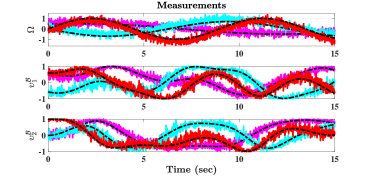
Figure 2: True values and measurements of $\Omega$, $\upsilon_{1}^{\mathcal{B}}$, and $\upsilon_{2}^{\mathcal{B}}$.

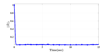
Figure 3: Tracking performance of normalized Euclidean distance error.

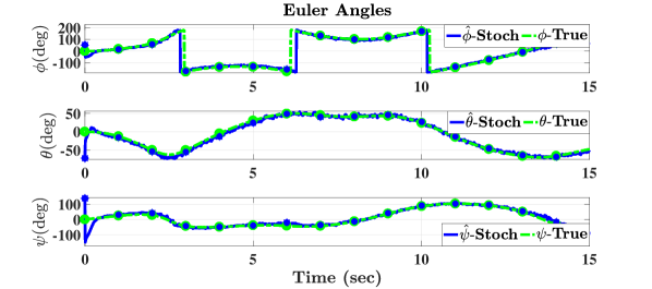
Figure 4: Tracking performance of Euler angles, proposed filter performance vs true trajectories.

Fig. 2 presents the true angular velocity $\left(\Omega\right)$ and true body-frame vectors as black centerlines and the associated high values of noise and bias components are represented by colored solid lines. The robustness of the filter against large initialization error and high values of noise and bias components is demonstrated in Fig. 3. The normalized Euclidean distance error $||\tilde{R}||_{I}$ was initiated very close to the unstable equilibria $\left(+1\right)$, eventually reduced to the neighborhood of the origin in probability as illustrated in Fig. 3. Fig. 4 illustrate the tracking performance of Euler angles, proposed filter performance vs true trajectories.

VI Conclusion

An explicit stochastic nonlinear attitude filter is proposed on $\mathbb{SO}\left(3\right)$. The proposed filter shares its structure with previously developed deterministic filters, but in stochastic sense. An alternate attitude potential function which has not been considered in literature, is introduced in this work. The resulting stochastic filter ensures that the errors in Rodriguez vector and estimates are semi-globally uniformly ultimately bounded in mean square. Numerical results show high convergence capabilities when large error is initialized in the attitude and high levels of noise and bias are observed in the vector measurements.

Appendix A

Proof of Lemma 1

Let the attitude be represented by $R\in\mathbb{SO}\left(3\right)$. From Section IV $\sum_{i=1}^{n}s_{i}=3$ which implies that ${\rm Tr}\left\{M^{\mathcal{I}}\right\}=3$ and the normalized Euclidean distance of $M^{\mathcal{I}}R$ is $\left\|M^{\mathcal{I}}R\right\|_{I}=\frac{1}{4}{\rm Tr}\left\{M^{\mathcal{I}}\left(\mathbf{I}_{3}-R\right)\right\}$. According to angle-axis parameterization in (2), one obtains

$$\left\|M^{\mathcal{I}}R\right\|_{I} =\frac{1}{4}{\rm Tr}\left\{-M^{\mathcal{I}}\left(\sin(\theta)\left[u\right]_{\times}+\left(1-\cos(\theta)\right)\left[u\right]_{\times}^{2}\right)\right\}$$

$$=-\frac{1}{4}{\rm Tr}\left\{M^{\mathcal{I}}\left(1-\cos(\theta)\right)\left[u\right]_{\times}^{2}\right\}$$ (60)

where ${\rm Tr}\left\{M^{\mathcal{I}}\left[u\right]_{\times}\right\}=0$ as given in identity (10). One has [21]

$$\left\|R\right\|_{I}=\frac{1}{4}{\rm Tr}\left\{\mathbf{I}_{3}-R\right\}={\rm sin}^{2}\left(\theta/2\right)$$ (61)

and the Rodriguez parameters vector in terms of angle-axis parameterization is [8] $u={\rm cot}\left(\theta/2\right)\rho$. From identity (8) $\left[u\right]_{\times}^{2}=-\left\|u\right\|^{2}\mathbf{I}_{3}+uu^{\top}$, the expression in (60) becomes

$$\left\|M^{\mathcal{I}}R\right\|_{I} =\frac{1}{2}\left\|R\right\|_{I}u^{\top}\bar{\mathbf{M}}^{\mathcal{I}}u=\frac{1}{2}\left\|R\right\|_{I}{\rm cot}^{2}\left(\frac{\theta}{2}\right)\rho^{\top}\bar{\mathbf{M}}^{\mathcal{I}}\rho$$

From (61), one can find ${\rm cos}^{2}\left(\frac{\theta}{2}\right)=1-\left\|R\right\|_{I}$ which means

$${\rm tan}^{2}\left(\frac{\theta}{2}\right)=\frac{\left\|R\right\|_{I}}{1-\left\|R\right\|_{I}}$$

Consequently, the normalized Euclidean distance is defined in the sense of Rodriguez parameters vector as

$$\left\|M^{\mathcal{I}}R\right\|_{I} =\frac{1}{2}\left(1-\left\|R\right\|_{I}\right)\rho^{\top}\bar{\mathbf{M}}^{\mathcal{I}}\rho=\frac{1}{2}\frac{\rho^{\top}\bar{\mathbf{M}}^{\mathcal{I}}\rho}{1+\left\|\rho\right\|^{2}}$$ (62)

This proves (19). The anti-symmetric projection operator can be defined in terms of Rodriquez parameters vector with the aid of identity (6) and (9) by

$$\boldsymbol{\mathcal{P}}_{a}\left(M^{\mathcal{I}}R\right)= \frac{M^{\mathcal{I}}\rho\rho^{\top}-\rho\rho^{\top}M^{\mathcal{I}}+M^{\mathcal{I}}\left[\rho\right]_{\times}+\left[\rho\right]_{\times}M^{\mathcal{I}}}{1+\left\|\rho\right\|^{2}}$$

$$= \frac{\left[\left({\rm Tr}\left\{M^{\mathcal{I}}\right\}\mathbf{I}_{3}-M^{\mathcal{I}}+\left[\rho\right]_{\times}M^{\mathcal{I}}\right)\rho\right]_{\times}}{1+\left\|\rho\right\|^{2}}$$

It follows that the vex operator of the above expression is

$$\Phi\left(M^{\mathcal{I}}R\right)=\mathcal{\mathbf{vex}}\left(\boldsymbol{\mathcal{P}}_{a}\left(M^{\mathcal{I}}R\right)\right) =\frac{\left(\mathbf{I}_{3}+\left[\rho\right]_{\times}\right)^{\top}}{1+\left\|\rho\right\|^{2}}\bar{\mathbf{M}}^{\mathcal{I}}\rho$$ (63)

This shows (20). The 2-norm of (63) can be obtained by

$$\left\|\Phi\left(M^{\mathcal{I}}R\right)\right\|^{2} =\frac{\rho^{\top}\bar{\mathbf{M}}^{\mathcal{I}}\left(\mathbf{I}_{3}-\left[\rho\right]_{\times}^{2}\right)\bar{\mathbf{M}}^{\mathcal{I}}\rho}{\left(1+\left\|\rho\right\|^{2}\right)^{2}}$$

with the aid of identity (8), one obtains

$$\left\|\Phi\left(M^{\mathcal{I}}R\right)\right\|^{2} =\frac{\rho^{\top}\bar{\mathbf{M}}^{\mathcal{I}}\left(\mathbf{I}_{3}-\left[\rho\right]_{\times}^{2}\right)\bar{\mathbf{M}}^{\mathcal{I}}\rho}{\left(1+\left\|\rho\right\|^{2}\right)^{2}}$$

$$=\frac{\rho^{\top}\left(\bar{\mathbf{M}}^{\mathcal{I}}\right)^{2}\rho}{1+\left\|\rho\right\|^{2}}-\frac{\left(\rho^{\top}\bar{\mathbf{M}}^{\mathcal{I}}\rho\right)^{2}}{\left(1+\left\|\rho\right\|^{2}\right)^{2}}$$

$$\geq\underline{\lambda}\left(1-\frac{\left\|\rho\right\|^{2}}{1+\left\|\rho\right\|^{2}}\right)\frac{\rho^{\top}\bar{\mathbf{M}}^{\mathcal{I}}\rho}{1+||\rho||^{2}}$$

$$\geq 2\underline{\lambda}\left(1-\left\|R\right\|_{I}\right)\left\|M^{\mathcal{I}}R\right\|_{I}$$ (64)

where $\underline{\lambda}=\underline{\lambda}\left(\bar{\mathbf{M}}^{\mathcal{I}}\right)$ and $\left\|R\right\|_{I}=\left\|\rho\right\|^{2}/\left(1+\left\|\rho\right\|^{2}\right)$ as defined in (4). It can be found that

$$1-\left\|R\right\|_{I} =\frac{1}{4}\left(1+{\rm Tr}\left\{\left(M^{\mathcal{I}}\right)^{-1}M^{\mathcal{I}}R\right\}\right)$$ (65)

Therefore, from (64), and (65) the following inequality holds

$$||\Phi\left(M^{\mathcal{I}}R\right)||^{2} \geq\frac{\underline{\lambda}}{2}\left(1+{\rm Tr}\left\{\left(M^{\mathcal{I}}\right)^{-1}M^{\mathcal{I}}R\right\}\right)\left\|M^{\mathcal{I}}R\right\|_{I}$$

which proves (21) in Lemma 1.

References

• [1] R. Mahony, T. Hamel, and J.-M. Pflimlin, “Nonlinear complementary filters on the special orthogonal group,” IEEE Transactions on Automatic Control, vol. 53, no. 5, pp. 1203–1218, 2008.
• [2] J. L. Crassidis, F. L. Markley, and Y. Cheng, “Survey of nonlinear attitude estimation methods,” Journal of guidance, control, and dynamics, vol. 30, no. 1, pp. 12–28, 2007.
• [3] D. Choukroun, I. Y. Bar-Itzhack, and Y. Oshman, “Novel quaternion kalman filter,” IEEE Transactions on Aerospace and Electronic Systems, vol. 42, no. 1, pp. 174–190, 2006.
• [4] E. J. Lefferts, F. L. Markley, and M. D. Shuster, “Kalman filtering for spacecraft attitude estimation,” Journal of Guidance, Control, and Dynamics, vol. 5, no. 5, pp. 417–429, 1982.
• [5] F. L. Markley, “Attitude error representations for kalman filtering,” Journal of guidance, control, and dynamics, vol. 26, no. 2, pp. 311–317, 2003.
• [6] J. L. Crassidis and F. L. Markley, “Unscented filtering for spacecraft attitude estimation,” Journal of guidance, control, and dynamics, vol. 26, no. 4, pp. 536–542, 2003.
• [7] M. S. Arulampalam, S. Maskell, N. Gordon, and T. Clapp, “A tutorial on particle filters for online nonlinear/non-gaussian bayesian tracking,” IEEE Transactions on Signal Processing, vol. 50, no. 2, pp. 174–185, 2002.
• [8] M. D. Shuster and S. D. Oh, “Three-axis attitude determination from vector observations,” Journal of Guidance, Control, and Dynamics, vol. 4, pp. 70–77, 1981.
• [9] D. E. Zlotnik and J. R. Forbes, “Nonlinear estimator design on the special orthogonal group using vector measurements directly,” IEEE Transactions on Automatic Control, vol. 62, no. 1, pp. 149–160, 2017.
• [10] H. F. Grip, T. I. Fossen, T. A. Johansen, and A. Saberi, “Attitude estimation using biased gyro and vector measurements with time-varying reference vectors,” IEEE Transactions on Automatic Control, vol. 57, no. 5, pp. 1332–1338, 2012.
• [11] H. A. Hashim, S. El-Ferik, and F. L. Lewis, “Adaptive synchronisation of unknown nonlinear networked systems with prescribed performance,” International Journal of Systems Science, vol. 48, no. 4, pp. 885–898, 2017.
• [12] H. A. Hashim, S. El-Ferik, and F. L. Lewis, “Neuro-adaptive cooperative tracking control with prescribed performance of unknown higher-order nonlinear multi-agent systems,” International Journal of Control, pp. 1–16, 2017.
• [13] M. D. Shuster, “A survey of attitude representations,” Navigation, vol. 8, no. 9, pp. 439–517, 1993.
• [14] R. Khasminskii, Stochastic stability of differential equations.   Rockville, MD: S & N International, 1980.
• [15] H. A. Hashim, L. J. Brown, and K. McIsaac, “Nonlinear stochastic attitude filters on the special orthogonal group 3: Ito and stratonovich,” IEEE Transactions on Systems, Man, and Cybernetics: Systems, pp. 1–13, 2018 (Submitted).
• [16] K. Ito and K. M. Rao, Lectures on stochastic processes.   Tata institute of fundamental research, 1984, vol. 24.
• [17] H. Deng, M. Krstic, and R. J. Williams, “Stabilization of stochastic nonlinear systems driven by noise of unknown covariance,” IEEE Transactions on Automatic Control, vol. 46, no. 8, pp. 1237–1253, 2001.
• [18] H.-B. Ji and H.-S. Xi, “Adaptive output-feedback tracking of stochastic nonlinear systems,” IEEE Transactions on Automatic Control, vol. 51, no. 2, pp. 355–360, 2006.
• [19] H. A. Hashim, L. J. Brown, and K. McIsaac, “Nonlinear stochastic position and attitude filter on the special euclidean group 3,” Journal of the Franklin Institute, pp. 1–27, 2018 (Submitted).
• [20] F. Bullo and A. D. Lewis, Geometric control of mechanical systems: modeling, analysis, and design for simple mechanical control systems.   Springer Science & Business Media, 2004, vol. 49.
• [21] R. M. Murray, Z. Li, S. S. Sastry, and S. S. Sastry, A mathematical introduction to robotic manipulation.   CRC press, 1994.