Abstract

In our study, we demonstrate the synergy effect between convolutional neural networks and the multiplicity of SMILES. The model we propose, the so-called Convolutional Neural Fingerprint (CNF) model, reaches the accuracy of traditional descriptors such as Dragon (Mauri et al. [22]), RDKit (Landrum [18]), CDK2 (Willighagen et al. [43]) and PyDescriptor (Masand and Rastija [20]). Moreover the CNF model generally performs better than highly fine-tuned traditional descriptors, especially on small data sets, which is of great interest for the chemical field where data sets are generally small due to experimental costs, the availability of molecules or accessibility to private databases. We evaluate the CNF model along with SMILES augmentation during both training and testing. To the best of our knowledge, this is the first time that such a methodology is presented. We show that using the multiplicity of SMILES during training acts as a regulariser and therefore avoids overfitting and can be seen as ensemble learning when considered for testing.

1 Introduction

Predicting molecular activities using machine learning algorithms such as deep neural networks is of high interest for chemical or pharmaceutical companies. Recent publications have shown the capacity of statistical learning to efficiently model chemical and biological phenomena at a molecular level with high accuracy (Baldi [4]).

One of the great challenges in chemoinformatics is to model a chemical structure. Indeed the physical and chemical aspects of these structures make for highly complex objects.

A chemical structure is often represented through the use of a connected and undirected graph, called molecular graph, which corresponds to the structural formula of the chemical compound. Vertices of the graph correspond to atoms of the molecule and edges to chemical bonds between these atoms.

From a computational point of view, a molecular graph remains a complex object and finding a numerical representation of a chemical structure is necessary in the context of machine learning. Consequently the concept of a fingerprint was developed. A fingerprint is a numerical representation which encodes molecular information (Todeschini et al. [40]). One of the reasons for developing fingerprints is to extract substructures from molecules. It is believed that molecules with similar groups of substructures will have similar properties (Muegge and Mukherjee [23]).

Another notation derived from the molecular graph is the Simplified Molecular Input Line Entry System (SMILES) suggested by Weininger [42]. SMILES is a linearisation of a given molecular graph, in the form of a single line text, obtained by enumerating nodes and edges following a certain topological ordering. Although SMILES encodes information on the local structure of the graph, a problem arises when linearising a graph. Cycle, branch and stereochemistry breaks can create ambiguities, especially in the training of a neural network.

A number of equally valid SMILES strings can be obtained for a single molecule since several topological orderings may exist for the corresponding graph. Indeed starting the enumeration from different nodes and following different paths of a molecular graph will lead to different SMILES representations of the same molecule. The number of possible SMILES grows with the complexity of the graph.

In order to have a one-to-one relationship between a molecule and its SMILES representation, some algorithms have been developed to choose one SMILES, called the canonical SMILES. There is no universal canonical SMILES since each toolkit has its own canonisation algorithm. Similar molecules do not necessarily have similar canonical SMILES representations.

The compact notation of SMILES allows for efficient numerical computation and is therefore used in this paper to predict molecular properties.

Widely used techniques to extract patterns in sequence modelling, such as SMILES, are Recurrent Neural Networks (RNN) and Convolutional Neural Network (CNN) (Bai et al. [3]). To account for ambiguities of cycle, branch and stereochemistry breaks, we suggest providing multiple versions of SMILES, which should be able to expose various views of the molecular graph and allow for a more global understanding of the structure of the chemical compound.

In this paper we expose a modelling approach of chemical structures inspired by the ResNet model by He et al. [12] which uses CNNs that combine both linear and hierarchical layers. Our contribution lies in the combination of CNN as a feature extraction method and the multiplicity of SMILES as a means to achieve data augmentation as suggested by Bjerrum [6].

2 Related work

In chemoinformatics, the use of SMILES as input for machine learning algorithms is not rare (Jastrzebski et al. [16], Olier et al. [26], Schwaller et al. [32]) and applying RNNs to SMILES has become more and more common. For example, Segler et al. [33] train RNNs as generative models for molecules and the deep RNN SMILES2vec model proposed by Goh et al. [10] is used to predict chemical properties.

In the framework of SMILES, Bjerrum [6] suggests that increasing the size of a dataset by considering several SMILES for one molecule is a way to achieve data augmentation. Previous publications have shown the effectiveness of data augmentation in deep learning applied to several different fields such as image classification (Perez and Wang [27]), time series classification (Ismail Fawaz et al. [15]), face recognition (Lv et al. [19]), relation classification (Xu et al. [45]) and soft biometrics classification (Romero Aquino et al. [30]). In this context, Goh et al. [11] took advantage of the multiplicity of SMILES in RNN models.

Although SMILES have been additionally processed through RNN architectures, we propose here to use CNNs, following Bai et al. [3] who have demonstrated the advantage of convolutional operators in sequence processing.

As an alternative to SMILES, recent research was conducted to define fingerprints directly from 2D molecular graphs, leading to neural fingerprints and the ConvGraph model, as proposed by Duvenaud et al. [9]. The idea behind neural fingerprints is to apply convolutions in order to obtain feature extraction. CNNs applied to string vectors have shown their effectiveness in different fields such as sentence classification, with the TextCNN model introduced by Kim [17].

Considering all of the above, we build a CNN model which acts as a feature extractor, leading to a neural fingerprint. We not only use SMILES as inputs but also take advantage of the multiplicity of SMILES as a means of obtaining data augmentation to cope with cycle, branch and stereochemistry breaks.

3 Convolutional Neural Fingerprint

In this section, we explain the Convolutional Neural Fingerprint (CNF) model, which heavily relies on the convolutional graph introduced by Duvenaud et al. [9], CNN for sentence classification (Kim [17]) and the architecture of the ResNet model suggested by He et al. [12].

The key ideas behind the convolutional graph are the hierarchical convolutional layers and a matrix multiplication which acts as a hash function. In the original paper by Duvenaud et al. [9], the convolutional graph operates directly on a molecular graph, which is known to be computationally inefficient. This is why we suggest implementing a CNN on the SMILES representation of a molecule. As a matter of fact, convolutional layers applied to string vectors have shown their effectiveness in sentence classification (Kim [17]) and SMILES are precisely single line characters which encode the information of a molecular graph.

The CNF model applies to the one-hot encoding of SMILES convolutional layers followed by matrix multiplications, which we denote $C$ c0pt0pt-0.2pt○ c-1.8pt0pt1.5pt+ $H$, where $H$ is an embedding matrix. The idea behind applying convolutional layers is to obtain neighbouring atoms in a chemical structure and multiplication can be interpreted as an embedding on a latent space. This $C$ c0pt0pt-0.2pt○ c-1.8pt0pt1.5pt+ $H$  implementation is highly linked to the Morgan fingerprint (Rogers and Hahn [29]), where on the one hand, relevant substructures, or neighbourhood of atoms, are encoded and on the other hand, features are hashed.

The architecture of the CNF model resembles the one of the ResNet model (He et al. [12]). Indeed both hierarchical and flat convolutional layers are used (see Figure 1(a)).

(a) Diagram of the CNF model following the ResNet architecture. The input $X$ is the one-hot encoding of a SMILES. $C$ $\mathrel{\raisebox{0.0pt}{{\small{\textbigcircle}}}}$​​​$\mathrel{\raisebox{2.2pt}{{\tiny{+}}}}$ $H$denotes a convolution plus a hashing layer.

(b) Diagram of the CNF model with flat convolutional layers. The input $X$ is the one-hot encoding of a SMILES. The first layer hashes $X$ without performing a convolution. The following layers use convolution, plus hashing, denoted $C$ $\mathrel{\raisebox{0.0pt}{{\small{\textbigcircle}}}}$​​​$\mathrel{\raisebox{2.2pt}{{\tiny{+}}}}$ $H$. After each layer, we sum the columns of the matrix, namely a pooling layer. Concatenating all these vectors leads to the neural fingerprint.

(c) Diagram of the CNF model with hierarchical convolutional layers. The input $X$ is the one-hot encoding of a SMILES. We apply a convolutional plus a hashing layer to $X$, denoted $C$ $\mathrel{\raisebox{0.0pt}{{\small{\textbigcircle}}}}$​​​$\mathrel{\raisebox{2.2pt}{{\tiny{+}}}}$ $H$. We obtain a first vector by summing the columns of the matrix, namely a pooling layer. The result of $C$ $\mathrel{\raisebox{0.0pt}{{\small{\textbigcircle}}}}$​​​$\mathrel{\raisebox{2.2pt}{{\tiny{+}}}}$ $H$is used as an input of the next layer, from which we obtain a second vector after pooling. Concatenating all these vectors leads to the neural fingerprint.

Figure 1: Diagram of the CNF model.

The neural fingerprint is obtained as follows: a pooling layer is applied to each $C$ c0pt0pt-0.2pt○ c-1.8pt0pt1.5pt+ $H$  operation, leading to a vector. For the CNF model, the pooling layer corresponds to summing the rows of the matrix $C$ c0pt0pt-0.2pt○ c-1.8pt0pt1.5pt+ $H$. Both the hashing $H$ and the pooling make for a nonlinear model. The neural fingerprint is obtained by concatenating all the vectors obtained after pooling. Figures 1(b) and 1(c) show the architecture of the CNF model in the case where the layers are strictly flat and strictly hierarchical, respectively.

An advantage of the CNF model is that it maps a sparse matrix, the one-hot encoding of a SMILES, into a dense vector, the neural fingerprint. The latter can be plugged directly into standard machine learning algorithms such as neural network, support vector machine and random forest. Duvenaud et al. [9] have shown that similar molecules have similar (in the Euclidian sense) neural fingerprints, even when the model has not been trained. In the CNF case, two SMILES with similar spelling will be close, in the Euclidian sense, in the latent space. This observation was already underlined in sentence classification when dealing with “semantically close words” (Kim [17]). In Section 7, we show the evolution of the distance matrix of the neural fingerprints as the CNF model trains (see Figure 7).

4 Data Augmentation

One of the main objectives of this research is to determine whether the multiplicity of SMILES can be used as means of providing data augmentation and therefore help the learning process of a neural network. The key idea behind data augmentation is to augment the number of observations from a given data set to obtain better performances when training machine learning algorithms.

One of the major risks when fitting a model is overfitting the data and this risk becomes greater when dealing with complex non-linear models, such as neural networks (Bishop [5], Tetko et al. [38]). Regularisation is a common way to prevent overfitting (Murphy [24]) and data augmentation is an effective technique of regularisation (Hernández-García and König [13]).

In chemoinformatics, Bjerrum [6] puts forward the idea of SMILES enumeration as a method of data augmentation. As mentioned previously, one molecule can have various SMILES representations. This multiplicity depends both on the atom where the enumeration starts and the path followed along the 2D graph of the molecular structure. Data are therefore created by exploring different directions of a given graph. Figure 2 shows the multiplicity of SMILES of the ethylcyclopropane molecule. We underline the fact that the two first SMILES have the same starting point, but the paths along the 2D graph are different and therefore lead to different SMILES.

The intuitive reason for believing that SMILES augmentation improves predictive performances is the following: a molecular graph is a cyclic graph, which contains all the structural information of a chemical compound, as a whole. However when constructing an associated SMILES, we choose to enumerate recursively the atoms present in the molecule in a certain sequence, which is equivalent to linearising a graph. Nevertheless information on the cyclic properties of the molecule is buried when using this line notation; a character indicating the beginning of a cycle or a branch may be separated from its closing character by many other strings, making the understanding of cycles difficult for a neural network. In this sense, SMILES are an acyclic graph of a molecule. Generating several valid SMILES, each with a different starting point and following different paths, will lead to different “spellings” of the same molecule, exposing many angles of the same item. By enumerating SMILES, we transfer the perspective from a local to a more global one. Similar to image classification, multiple SMILES allow for several views of the same object.

In our simulations, we make the distinction between the augmentation of SMILES during training and the augmentation during inference. Indeed both Bjerrum [6] and Schwaller et al. [32] have shown the effectiveness of SMILES augmentation during training. However, to our knowledge, no simulations have been performed using SMILES augmentation during both training and testing.

SMILES augmentation during testing can be regarded as ensemble learning. When provided with one molecule, we generate several valid SMILES along with their respective model outputs. The aggregation of the outputs allows for a consensus effect. In the regression case, the outputs are averaged whereas in the classification case, the classification is done based on the majority vote of the different outputs.

The results of the simulations in the next section show that the technique of SMILES augmentation during training and testing improves predictive performances.

Figure 2: Consider the molecule ethylcyclopropane given by the chemical formula C5H10. The figure illustrates the 2D and SMILES representation of the molecule. Four diagrams are displayed. In each diagram, the arrow points at the atom where the enumeration starts for the SMILES construction. The path along the 2D graph can be followed with the numbers starting at 1 next to the nodes. All four SMILES are equally valid for this molecular structure.

5 Results

In this section we discuss the results of our simulations, which are performed on OCHEM (Sushko et al. [34]), an online chemical modelling platform, which itself uses the Python library DeepChem (Ramsundar et al. [28]) and the open source chemoinformatics software RDKit (Landrum [18]). We stress here the fact that a new RDKit feature has been developed to generate all possible valid SMILES. The function that had been implemented previously did not enumerate all possible valid SMILES due to restrictions in some of the enumeration rules. Computational tasks were performed on NVIDIA cards. The code is available upon request in both Tensorflow (Abadi et al. [1]) and Matlab (MATLAB [21]).

First we discuss how SMILES augmentation influences the CNF model and then we compare the best performances of the CNF model with existing models, such as deep neural networks (DNN) (Wu et al. [44]), ConvGraph (Altae-Tran et al. [2]) and TextCNN (Kim [17]) already implemented on OCHEM. When available, we use the benchmark results presented by Wu et al. [44].

The CNF model along with SMILES augmentation is performed on several data sets, including both regression and classification tasks. The data were obtained from open source data bases, which are all available on OCHEM. In the regression setting, predictions are made on targets such as the MP, melting point (Tetko et al. [39]), the BP, boiling point (Brandmaier et al. [7]), the BCF, bioconcentration factor (Brandmaier et al. [7]), FreeSolv, free solvation (Wu et al. [44]), LogS (Delaney [8]), Lipo, lipophilicity (Huuskonen et al. [14]), BACE (Wu et al. [44]), the DHFR, dihydrofolate reductase inhibition (Sutherland and Weaver [36]) and the LEL, lowest effect level (Novotarskyi et al. [25]). We choose the Root Mean Square Error (RMSE) as a measure of comparison.

For classification, we test the following: HIV (Wu et al. [44]), AMES (Sushko et al. [35]), BACE (Wu et al. [44]), Clintox (Wu et al. [44]), Tox21 (Wu et al. [44]), the BBBP, blood-brain barrier penetration (Wu et al. [44]), JAK3 (Suzuki et al. [37]), BioDeg (Vorberg and Tetko [41]) and RP AR (Rybacka et al. [31]), and compare them using the AUC (Area Under the Curve) measure. These sets include small sizes (of order 1e2), medium sizes (of order 1e3) and larger sizes (of order 1e4), as shown in Table 1.

In order to efficiently test the performances of the models, we use 5-fold cross-validation. The splitting of the data was done before the augmentation of SMILES. In order to test the effect of SMILES augmentation on the CNF model, we compare the following:

1. No augmentation on SMILES. We leave both train and test sets unchanged, for which we use the notation: SMILES 1/1. The considered SMILES are the canonical version.

2. SMILES augmentation during training only. If we generate $n$ random SMILES in the train set, where $n\in\mathbb{N}$, but leave the test set unchanged, we use the notation: SMILES n/1. The SMILES in the test set are the canonical versions.

3. SMILES augmentation during testing only. If we generate $m$ random SMILES in the test set, where $m\in\mathbb{N}$, but leave the train set unchanged, we note: SMILES 1/m. The SMILES in the train set are the canonical versions.

4. SMILES augmentation during both training and testing. If we generate $n$ random SMILES in the train set and $m$ random SMILES in the test set, where $n,m\in\mathbb{N}$, we note: SMILES n/m.

The results of the simulations to test the effect of SMILES augmentation are detailed in Table 1. Based on the illustration of these results displayed in Figures 3 and 4, we make the following observations. Augmenting during training (SMILES n/1) almost always improves predictive performances compared to leaving the data set untouched (SMILES 1/1). This observation confirms that SMILES augmentation during training can be interpreted as data augmentation, as discussed in Section 4. Augmenting during testing only (SMILES 1/m) almost always worsens the performances compared to leaving the data set untouched (SMILES 1/1). This shows that the CNF model is only able to map the SMILES to one instance of the enumeration and not to the original graph. In our implementation, the input SMILES are canonical and the CNF model received non-canonical SMILES for prediction. In this case, the neural network is confronted to new data, which it never had the opportunity to train on, leading to poor predictive power.

The situation where the best results are obtained is when both augmentation during training and testing is implemented. There is not only a data augmentation effect which acts on the train set but there is also an ensemble learning effect on the test set, as discussed in Section 4.

We choose the best models from Table 1 and compare the results with the models that give the best results in Deepchem (Wu et al. [44]). Please refer to Table 2 for the results. We notice that in most cases, the CNF model performs at least as well as the best Deepchem models.

Tables 3 and 4 list the results of classification and regression tasks respectively using models available on OCHEM, where the simulations were done with the default parameters. Figures 5 and 6 give an illustration of these results. We notice that in most cases the CNF model provides better accuracy compared to models built using the best descriptors and computational methods.

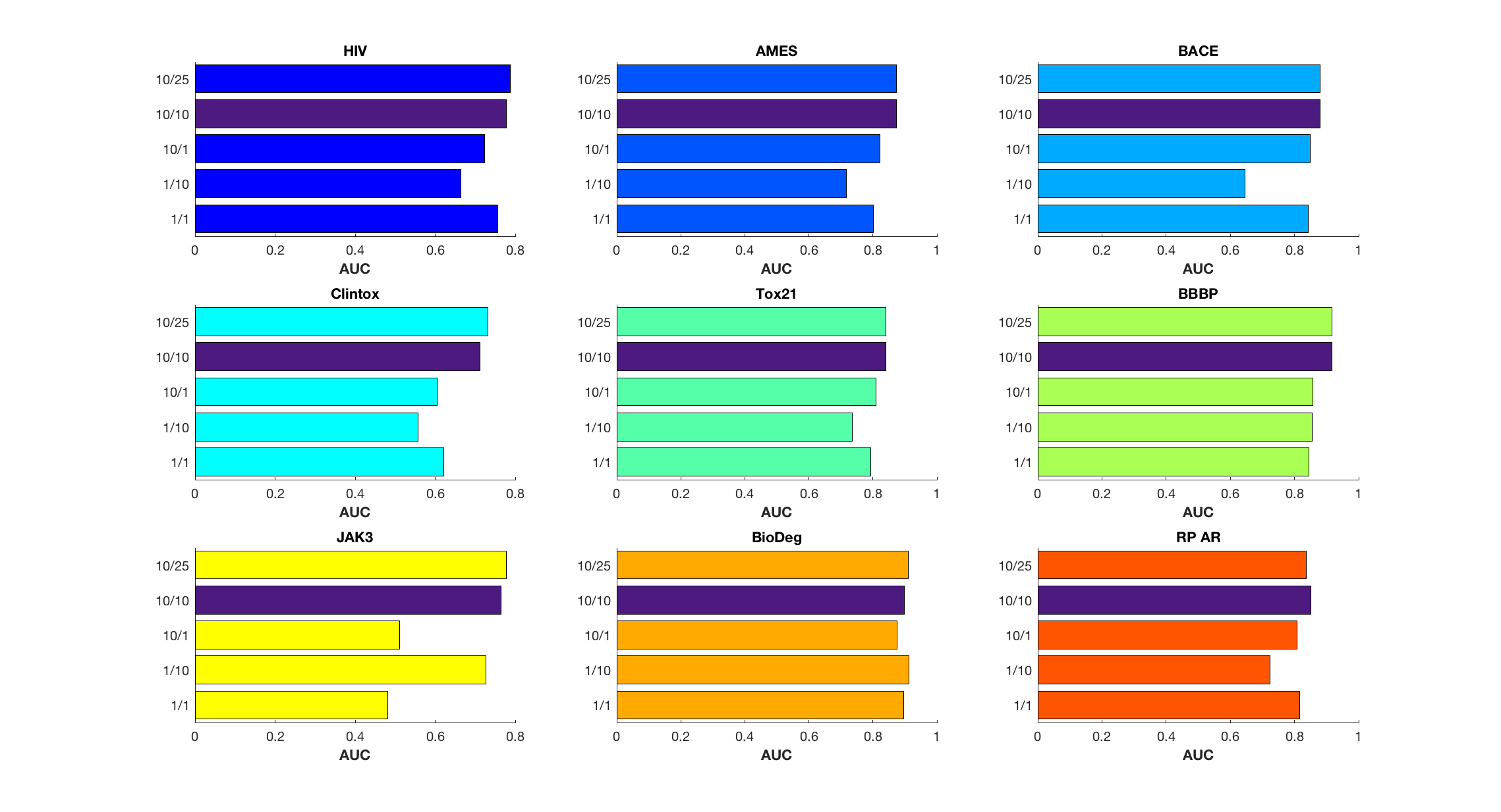
Figure 3: The evaluation of the CNF model along with SMILES enumeration for classification tasks. Enumeration is done during training only (SMILES 10/1), testing only (SMILES (1/10), both (SMILES 10/10 and SMILES 10/25) or none (SMILES 1/1). The default parameter (SMILES 10/10) is displayed in purple. The higher the AUC value, the better the performance. The figure indicates that augmentation during training and testing (SMILES 10/10 or SMILES 10/25) certainly improves the accuracy of the CNF model.

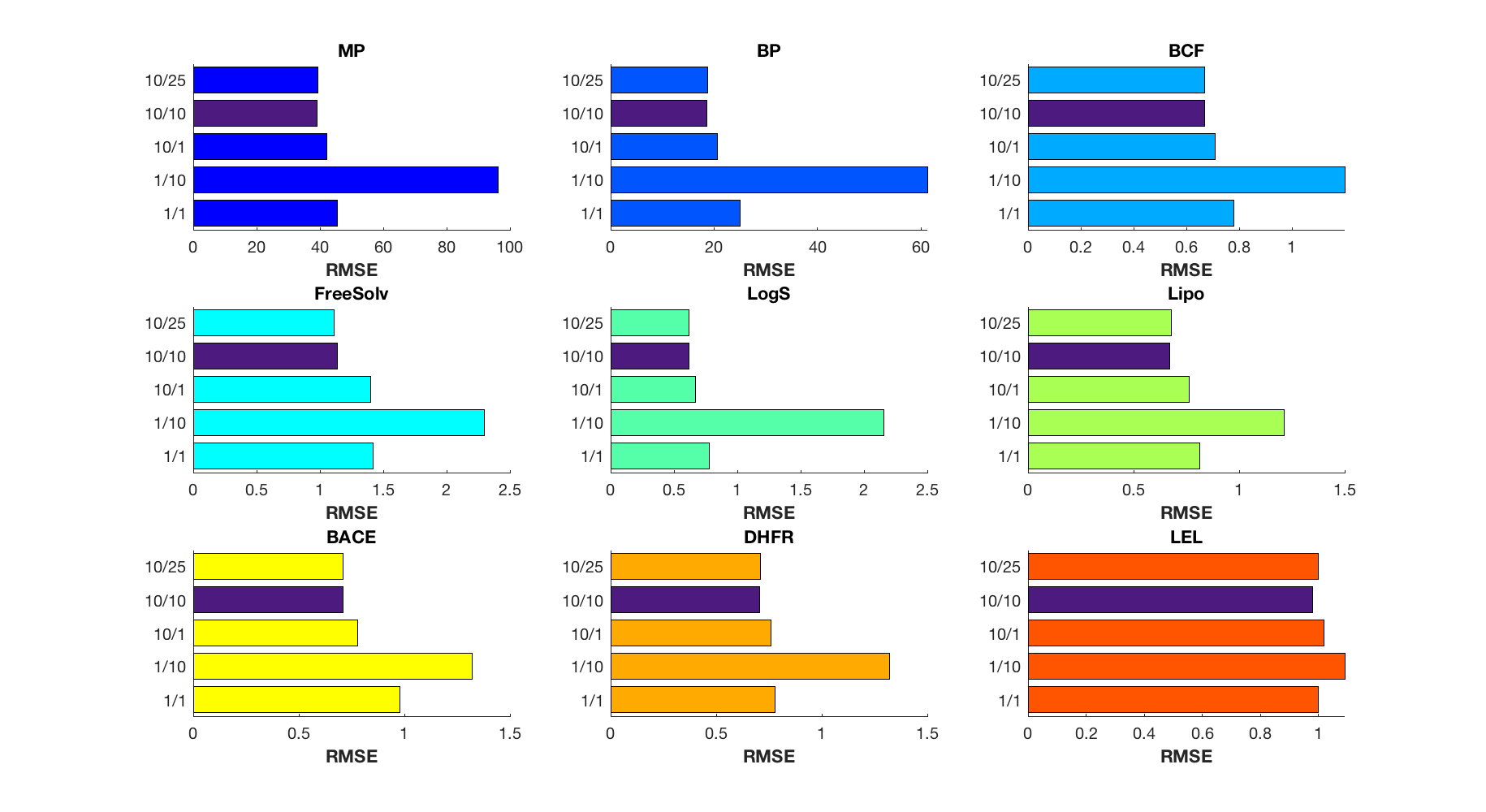
Figure 4: The evaluation of the CNF model along with SMILES enumeration for regression tasks. Enumeration is done during training only (SMILES 10/1), testing only (SMILES (1/10), both (SMILES 10/10 and SMILES 10/25) or none (SMILES 1/1). The default parameter (SMILES 10/10) is displayed in purple. The lower the RMSE value, the better the performance. The figure indicates that augmentation during training and testing (SMILES 10/10 or SMILES 10/25) certainly improves the accuracy of the CNF model.

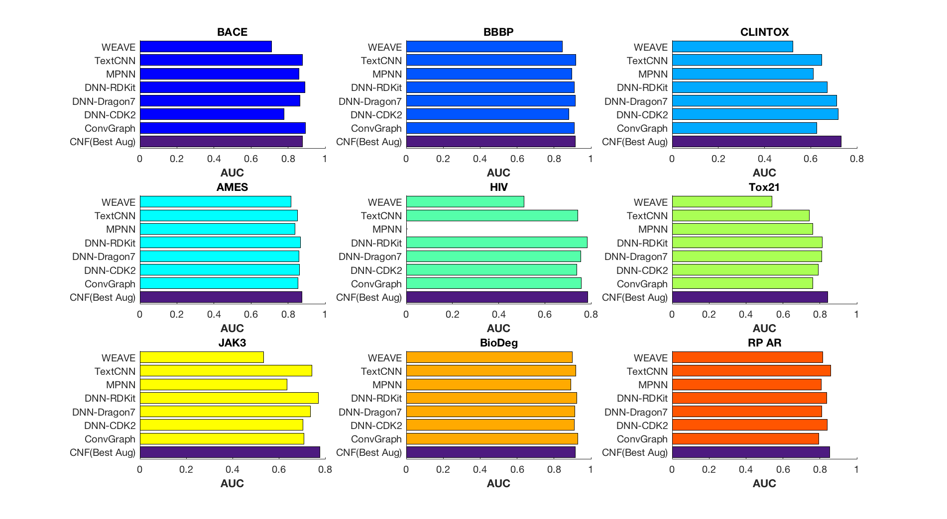
Figure 5: Comparison of the best CNF model and other existing models for classification tasks. The best CNF model is displayed in purple. The higher the AUC value, the better the performance. The figure indicates that the CNF model provides better accuracy compared to models built using the best descriptors and computational methods.

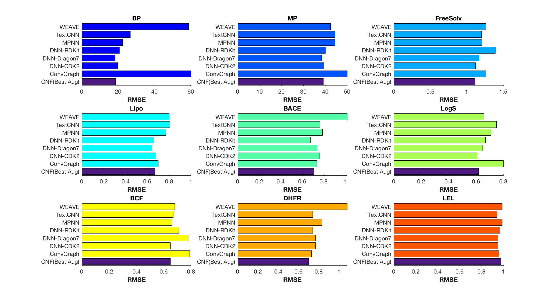
Figure 6: Comparison of the best CNF model and other existing models for regression tasks. The best CNF model is displayed in purple. The lower the RMSE value, the better the performance. The figure indicates that the CNF model provides better accuracy compared to models built using the best descriptors and computational methods.

6 Conclusion and Future Work

In this study, we apply machine learning algorithms on SMILES, which is a convenient linear graph notation containing information of a molecular structure. It is well known that there are many valid SMILES for a given molecule. The model we propose, namely the Convolutional Neural Fingerprint (CNF) model, seems to be able to extract the information about the local structure of a chemical compound thanks to convolutional layers. Using the multiplicity of SMILES as means of data augmentation also allows the CNF model to learn about the global structure. SMILES augmentation improves the CNF model predictions by approximately 15% (and in the best of cases by approximately 25%) which is enough to reach conventional human descriptor performances, such as the well known CDK2, Dragon or RDKit. These performances are observed on difficult target values such as the melting point of a molecular structure.

Currently we have investigated molecular QSAR/QSPR (quantitative structure-activity/ property relationship) models. One of our objectives is to use the CNF model to also predict quantum chemistry atomic targets.

Another goal would be to apply augmentation not only on the prediction of molecular behaviour as we have tested but as well on reaction tasks.

The ensemble learning resulting from the augmentation during testing helps provide a metric to determine if a SMILES is in the applicability domain of the model. The mean and variance can provide information on the quality of the model. This approach is already implemented in OCHEM but has not been fully investigated.

Augmentation during training and testing is also under investigation for the TextCNN model.

Acknowledgements

Talia Kimber would like to thank Eric Bruno, Guillaume Godin and Sebastian Engelke for their support and dedication in supervising this project which is part of her Master’s Thesis.
Sebastian Engelke is grateful for financial support of the Swiss National Science Foundation.
Guillaume Godin thanks Greg Landrum, Esben J. Bjerrum and Takayuki Serizawa for the RDKit UGM Hackathon which took place in Cambridge in September 2018.
Guillaume Godin is grateful for the improvements made by Arvind Jayaraman on the MathWorks’ deep learning toolbox.
The authors thank Alpha A. Lee as well as Philippe Schwaller for beneficial discussions.

7 Supplementary Material

Target Size Augmentation RMSE MP 1 9104 1/1 45.6 10/1 42.8 1/10 96.2 10/10 39.2 10/25 39.0 BP 1 1893 1/1 25.0 10/1 20.7 1/10 61.2 10/10 18.6 10/25 18.6 BCF 378 1/ 1 0.78 10/1 0.71 1/10 1.20 10/10 0.65 10/25 0.65 FreeSolv 642 1/ 1 1.42 10/1 1.40 1/10 2.30 10/10 1.14 10/25 1.11 LogS 1 311 1/ 1 0.78 10/1 0.67 1/10 2.16 10/10 0.62 10/25 0.62 Lipo 4 200 1/ 1 0.81 10/1 0.76 1/10 1.21 10/10 0.67 10/25 0.68 BACE 1 513 1/ 1 0.98 10/1 0.78 1/10 1.32 10/10 0.71 10/25 0.71 DHFR 739 1/ 1 0.78 10/1 0.76 1/10 1.32 10/10 0.70 10/25 0.71 LEL 483 1/ 1 1.0 10/1 1.0 1/10 1.1 10/10 1.0 10/25 1.0

Target Size Augmentation AUC HIV 4 1127 1/1 0.76 10/1 0.72 1/10 0.67 10/10 0.78 10/25 0.79 AMES 6 542 1/ 1 0.80 10/ 1 0.82 1/10 0.72 10/10 0.87 10/25 0.87 BACE 1 513 1/ 1 0.84 10/1 0.85 1/10 0.65 10/10 0.88 10/25 0.88 Clintox 1 478 1/ 1 0.62 10/1 0.61 1/10 0.56 10/10 0.71 10/25 0.73 Tox21 7 831 1/ 1 0.79 10/1 0.81 1/10 0.74 10/10 0.84 10/25 0.84 BBBP 2 039 1/ 1 0.84 10/1 0.86 1/10 0.86 10/10 0.92 10/25 0.92 JAK3 886 1/ 1 0.48 10/1 0.51 1/10 0.73 10/10 0.76 10/25 0.78 BioDeg 1 737 1/ 1 0.90 10/1 0.88 1/10 0.91 10/10 0.90 10/25 0.91 RP AR 930 1/ 1 0.82 10/1 0.81 1/10 0.72 10/10 0.85 10/25 0.83

Table 1: Summary of the results of the simulations using the CNF model with the multiplicity of SMILES. The first column represents the target value (the left and right tables consider regression and classification tasks, respectively). The second column represents the size of the initial data set. The third column shows the type of augmentation that is performed on the data set, and the last column is the measure chosen to compare the performance of the CNF model, namely the RMSE and the AUC in regression and classification tasks, respectively. The augmentation which gives the best result is displayed in bold, indicating that augmentation during training and testing (SMILES 10/10 or SMILES 10/25) certainly improves the accuracy of the model.

Target Model Performance (RMSE) MP CNF 39.2 Deepchem NA BP CNF 18.6 Deepchem NA BCF CNF 0.65 Deepchem NA FreeSolv CNF 1.11 MPNN 1.15 LogS CNF 0.62 Deepchem NA Lipo CNF 0.671 ConvGraph 0.66 BACE CNF 0.71 Deepchem NA DHFR CNF 0.7 Deepchem NA LEL CNF 1 Deepchem NA

Target Model Performance (AUC) HIV CNF 0.79 KernelSVM 0.792 AMES CNF 0.87 Deepchem NA BACE CNF 0.88 RF 0.867 Clintox CNF 0.73 Weave 0.832 Tox21 CNF 0.84 ConvGraph 0.829 BBBP CNF 0.92 KernelSVM 0.729 JAK3 CNF 0.78 Deepchem NA BioDeg CNF 0.92 Deepchem NA RP AR CNF 0.85 Deepchem NA

Table 2: Comparison of the best CNF model with best results in Deepchem (Wu et al. [44]), using regression tasks (left table) and classification tasks (right table). The first column represents the target value. The second column lists the models. The third column shows the performance of each model. The best model is displayed in bold, indicating that the best CNF model usually performs better than the best Deepchem model.

Target Model (5 CV) AUC HIV CNF 0.79 ConvGraph 0.76 TextCNN 0.74 MPNN NA Weave 0.51 DNN (Dragon7) 0.76 DNN (CDK2) 0.74 DNN (RDKit) 0.78 DNN (PyDescriptor) 0.77 AMES CNF 0.87 ConvGraph 0.85 TextCNN 0.85 MPNN 0.84 Weave 0.82 DNN (Dragon7) 0.86 DNN (CDK2) 0.86 DNN (RDKit) 0.87 DNN (PyDescriptor) 0.86 BACE CNF 0.88 ConvGraph 0.89 TextCNN 0.88 MPNN 0.86 Weave 0.71 DNN (Dragon7) 0.87 DNN (CDK2) 0.78 DNN (RDKit) 0.89 DNN (PyDescriptor) 0.86

Target Model (5 CV) AUC Clintox CNF 0.73 ConvGraph 0.63 TextCNN 0.65 MPNN 0.61 Weave 0.52 DNN (Dragon7) 0.71 DNN (CDK2) 0.72 DNN (RDKit) 0.67 DNN (PyDescriptor) 0.71 Tox21 CNF 0.84 ConvGraph 0.76 TextCNN 0.74 MPNN 0.76 Weave 0.54 DNN (Dragon7) 0.81 DNN (CDK2) 0.79 DNN (RDKit) 0.81 DNN (PyDescriptor) 0.81 BBBP CNF 0.92 ConvGraph 0.91 TextCNN 0.92 MPNN 0.90 Weave 0.84 DNN (Dragon7) 0.92 DNN (CDK2) 0.88 DNN (RDKit) 0.91 DNN (PyDescriptor) 0.91

Target Model (5 CV) AUC JAK3 CNF 0.78 ConvGraph 0.71 TextCNN 0.74 MPNN 0.64 Weave 0.53 DNN (Dragon7) 0.74 DNN (CDK2) 0.71 DNN (RDKit) 0.77 DNN (PyDescriptor) 0.76 BioDeg CNF 0.92 ConvGraph 0.93 TextCNN 0.92 MPNN 0.89 Weave 0.90 DNN (Dragon7) 0.91 DNN (CDK2) 0.91 DNN (RDKit) 0.92 DNN (PyDescriptor) 0.91 RP AR CNF 0.85 ConvGraph 0.80 TextCNN 0.85 MPNN 0.81 Weave 0.82 DNN (Dragon7) 0.81 DNN (CDK2) 0.84 DNN (RDKit) 0.84 DNN (PyDescriptor) 0.83

Table 3: Comparison of the best CNF model with results on OCHEM, using 5-fold cross-validation on 9 classification tasks; HIV, AMES and BACE in the first table, Clintox, Tox21 and BBBP in the second table and JAK3, BioDeg and RP AR in the third table. The first column represents the target value. The second column lists the models. The third column shows the AUC, Area Under the Curve, value. The top-performing models which are shown in bold clearly demonstrate that the CNF model provides better accuracy compared to models built using the best descriptors and computational methods.

Target Model (5 CV) RMSE MP CNF 39.2 ConvGraph 50.0 TextCNN 44.5 MPNN 44.4 Weave 42.4 DNN (Dragon7) 38.4 DNN (CDK2) 39.4 DNN (RDKit) 40.0 DNN (PyDescriptor) 41.0 BP CNF 18.6 ConvGraph 60.2 TextCNN 26.8 MPNN 22.4 Weave 58.8 DNN (Dragon7) 18.3 DNN (CDK2) 19.8 DNN (RDKit) 20.8 DNN (PyDescriptor) 18.1 BCF CNF 0.65 ConvGraph 0.79 TextCNN 0.68 MPNN 0.66 Weave 0.68 DNN (Dragon7) 0.78 DNN (CDK2) 0.65 DNN (RDKit) 0.71 DNN (PyDescriptor) 0.66

Target Model (5 CV) RMSE FreeSolv CNF 1.11 ConvGraph 1.26 TextCNN 1.20 MPNN 1.21 Weave 1.26 DNN (Dragon7) 1.17 DNN (CDK2) 1.12 DNN (RDKit) 1.39 DNN (PyDescriptor) 1.09 LogS CNF 0.62 ConvGraph 0.80 TextCNN 0.74 MPNN 0.71 Weave 0.66 DNN (Dragon7) 0.65 DNN (CDK2) 0.61 DNN (RDKit) 0.67 DNN (PyDescriptor) 0.63 Lipo CNF 0.67 ConvGraph 0.70 TextCNN 0.81 MPNN 0.77 Weave 0.80 DNN (Dragon7) 0.65 DNN (CDK2) 0.68 DNN (RDKit) 0.66 DNN (PyDescriptor) 0.65

Target Model (5 CV) RMSE BACE CNF 0.71 ConvGraph 0.74 TextCNN 0.77 MPNN 0.79 Weave 1.02 DNN (Dragon7) 0.74 DNN (CDK2) 0.76 DNN (RDKit) 0.68 DNN (PyDescriptor) 0.72 DHFR CNF 0.70 ConvGraph 0.73 TextCNN 0.74 MPNN 0.83 Weave 1.08 DNN (Dragon7) 0.77 DNN (CDK2) 0.77 DNN (RDKit) 0.74 DNN (PyDescriptor) 0.76 LEL CNF 0.98 ConvGraph 0.96 TextCNN 0.94 MPNN 0.99 Weave 0.99 DNN (Dragon7) 0.95 DNN (CDK2) 0.95 DNN (RDKit) 0.97 DNN (PyDescriptor) 1.02

Table 4: Comparison of the best CNF model with results in OCHEM, using 5-fold cross-validation on 9 regression tasks; MP, BP and BCF in the first table, FreeSolv, LogS and Lipo in the second table and BACE, DHFR and LEL in the third table. The first column represents the target value. The second column lists the models. The third column shows the RSME, Root Mean Square Error, value. The top-performing models which are shown in bold clearly demonstrate that the CNF model provides better accuracy compared to models built using the best descriptors and computational methods.

Let $S_{1},\dots,S_{N}$ be $N$ initial SMILES of a given data set and suppose that for each SMILES, we generate $n$ random SMILES, namely

$$S_{1}^{1},\dots,S_{1}^{n},S_{2}^{1},…S_{2}^{n},\dots,S_{N}^{1},\dots,S_{N}^{n}.$$

Suppose we consider the CNF model with only one convolutional layer. For $i=1,\dots,N$ and $j=1,\dots,n$, let $\operatorname{NFP}_{i}^{j}$ be the neural fingerprint associated with the $j^{th}$ generated SMILES of the $i^{th}$ initial SMILES. Then we expect that the CNF model learns that $\forall i,l\in\{1,\dots,N\},\,\forall j,k,m\in\{1,\dots n\}$

$$||\operatorname{NFP}_{i}^{j}-\operatorname{NFP}_{i}^{k}||_{2}^{2}\leq||\operatorname{NFP}_{i}^{j}-\operatorname{NFP}_{l}^{m}||_{2}^{2},$$

that is the Euclidian distance between neural fingerprints generated by the same SMILES is smaller or equal than the Euclidian distance between neural fingerprints generated by two different SMILES.

The following results give us reason to believe that the statement above is true. Let $D_{1}$ and $D_{10}\in\mathbb{R}^{Nn\times Nn}$ be the distance matrices obtained after one and ten epochs respectively (see Figure 7). We notice that as the CNF model trains, the Euclidian distance between neural fingerprints generated by the same SMILES is smaller than the Euclidian distance between neural fingerprints generated by two different SMILES.

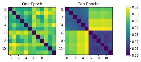
(a) Close up of the distance matrix $D$ after one and ten epochs respectively of the CNF model, namely $D_{1}$ and $D_{10}$. We notice the creation of two main clusters after ten epochs.

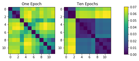
(b) Different close up of the distance matrix $D$ after one and ten epochs respectively of the CNF model, namely $D_{1}$ and $D_{10}$. We notice the creation of three main clusters after ten epochs.

Figure 7: Suppose we generate $n$ random SMILES from a data set of size $N$. For $i=1,\dots,N$ and $j=1,\dots,n$, let $\operatorname{NFP}_{i}^{j}$ be the neural fingerprint associated with the $j^{th}$ generated SMILES of the $i^{th}$ initial SMILES, obtained with the CNF model. Let $D_{1},D_{10}$ be the Euclidian distance matrices associated with all NFPs after one and ten epochs, respectively. Figure 7(a) and 7(b) show a close up of $D_{1}$ and $D_{10}$. We notice that as the CNF model trains, the Euclidian distance between neural fingerprints generated by the same SMILES is smaller than the Euclidian distance between neural fingerprints generated by two different SMILES.

References

- Abadi et al. [2015] Abadi, M., Agarwal, A., Barham, P., Brevdo, E., Chen, Z., Citro, C., Corrado, G. S., Davis, A., Dean, J., Devin, M., Ghemawat, S., Goodfellow, I., Harp, A., Irving, G., Isard, M., Jia, Y., Jozefowicz, R., Kaiser, L., Kudlur, M., Levenberg, J., Mané, D., Monga, R., Moore, S., Murray, D., Olah, C., Schuster, M., Shlens, J., Steiner, B., Sutskever, I., Talwar, K., Tucker, P., Vanhoucke, V., Vasudevan, V., Viégas, F., Vinyals, O., Warden, P., Wattenberg, M., Wicke, M., Yu, Y. and Zheng, X. (2015) TensorFlow: Large-scale machine learning on heterogeneous systems. Software available from tensorflow.org.
- Altae-Tran et al. [2016] Altae-Tran, H., Ramsundar, B., Pappu, A. S. and Pande, V. S. (2016) Low data drug discovery with one-shot learning. CoRR abs/1611.03199.
- Bai et al. [2018] Bai, S., Kolter, J. Z. and Koltun, V. (2018) An empirical evaluation of generic convolutional and recurrent networks for sequence modeling. CoRR abs/1803.01271.
- Baldi [2018] Baldi, P. (2018) Deep learning in biomedical data science. Annual Review of Biomedical Data Science 1(1), 181–205.
- Bishop [1995] Bishop, C. (1995) Neural networks for pattern recognition. Oxford University Press, USA.
- Bjerrum [2017] Bjerrum, E. J. (2017) SMILES enumeration as data augmentation for neural network modeling of molecules. CoRR abs/1703.07076.
- Brandmaier et al. [2012] Brandmaier, S., Sahlin, U., Tetko, I. V. and Öberg, T. (2012) Pls-optimal: a stepwise d-optimal design based on latent variables. Journal of chemical information and modeling 52(4), 975—983.
- Delaney [2004] Delaney, J. S. (2004) Esol: Estimating aqueous solubility directly from molecular structure. Journal of Chemical Information and Computer Sciences 44(3), 1000–1005. PMID: 15154768.
- Duvenaud et al. [2015] Duvenaud, D., Maclaurin, D., Aguilera-Iparraguirre, J., Gómez-Bombarelli, R., Hirzel, T., Aspuru-Guzik, A. and Adams, R. P. (2015) Convolutional Networks on Graphs for Learning Molecular Fingerprints. ArXiv e-prints .
- Goh et al. [2017a] Goh, G. B., Hodas, N. O., Siegel, C. and Vishnu, A. (2017a) SMILES2Vec: An Interpretable General-Purpose Deep Neural Network for Predicting Chemical Properties. ArXiv e-prints p. arXiv:1712.02034.
- Goh et al. [2017b] Goh, G. B., Siegel, C., Vishnu, A. and Hodas, N. O. (2017b) Using Rule-Based Labels for Weak Supervised Learning: A ChemNet for Transferable Chemical Property Prediction. ArXiv e-prints .
- He et al. [2015] He, K., Zhang, X., Ren, S. and Sun, J. (2015) Deep residual learning for image recognition. CoRR abs/1512.03385.
- Hernández-García and König [2018] Hernández-García, A. and König, P. (2018) Data augmentation instead of explicit regularization. ArXiv e-prints .
- Huuskonen et al. [2000] Huuskonen, J. J., Livingstone, D. J. and Tetko, I. V. (2000) Neural network modeling for estimation of partition coefficient based on atom-type electrotopological state indices. Journal of Chemical Information and Computer Sciences 40(4), 947–955. PMID: 10955523.
- Ismail Fawaz et al. [2018] Ismail Fawaz, H., Forestier, G., Weber, J., Idoumghar, L. and Muller, P.-A. (2018) Data augmentation using synthetic data for time series classification with deep residual networks. ArXiv e-prints .
- Jastrzebski et al. [2016] Jastrzebski, S., Lesniak, D. and Czarnecki, W. M. (2016) Learning to SMILE(S). CoRR abs/1602.06289.
- Kim [2014] Kim, Y. (2014) Convolutional neural networks for sentence classification. In EMNLP.
- Landrum [2016] Landrum, G. (2016) Rdkit: Open-source cheminformatics software .
- Lv et al. [2017] Lv, J.-J., Shao, X.-H., Huang, J.-S., Zhou, X.-D. and Zhou, X. (2017) Data augmentation for face recognition. Neurocomput. 230(C), 184–196.
- Masand and Rastija [2017] Masand, V. H. and Rastija, V. (2017) PyDescriptor : A new PyMOL plugin for calculating thousands of easily understandable molecular descriptors. Chemometrics and Intelligent Laboratory Systems 169, 12–18.
- MATLAB [2010] MATLAB (2010) version 7.10.0 (R2010a). Natick, Massachusetts: The MathWorks Inc.
- Mauri et al. [2006] Mauri, A., Consonni, V., Pavan, M. and Todeschini, R. (2006) Dragon software: An easy approach to molecular descriptor calculations. MATCH Communications in Mathematical and in Computer Chemistry 56, 237–248.
- Muegge and Mukherjee [2016] Muegge, I. and Mukherjee, P. (2016) An overview of molecular fingerprint similarity search in virtual screening. Expert Opinion on Drug Discovery 11(2), 137–148. PMID: 26558489.
- Murphy [2012] Murphy, K. (2012) Machine Learning: a Probabilistic Perspective. MIT Press.
- Novotarskyi et al. [2016] Novotarskyi, S., Abdelaziz, A., Sushko, Y., Körner, R., Vogt, J. and Tetko, I. V. (2016) Toxcast epa in vitro to in vivo challenge: Insight into the rank-i model. Chemical research in toxicology 29(5), 768—775.
- Olier et al. [2017] Olier, I., Sadawi, N., Bickerton, G. R. J., Vanschoren, J., Grosan, C., Soldatova, L. N. and King, R. D. (2017) Meta-qsar: a large-scale application of meta-learning to drug design and discovery. CoRR abs/1709.03854.
- Perez and Wang [2017] Perez, L. and Wang, J. (2017) The effectiveness of data augmentation in image classification using deep learning. CoRR abs/1712.04621.
- Ramsundar et al. [2016] Ramsundar, B., Pande, V., Eastman, P., Feinberg, E., Gomes, J., Leswing, K., Pappu, A. and Wu, M. (2016) Democratizing deep-learning for drug discovery, quantum chemistry, materials science and biology.
- Rogers and Hahn [2010] Rogers, D. and Hahn, M. (2010) Extended-connectivity fingerprints. Journal of Chemical Information and Modeling 50(5), 742–754. PMID: 20426451.
- Romero Aquino et al. [2017] Romero Aquino, N., Gutoski, M., Hattori, L. and Lopes, H. (2017) The effect of data augmentation on the performance of convolutional neural networks.
- Rybacka et al. [2015] Rybacka, A., Ruden, C., Tetko, I. V. and Andersson, P. L. (2015) Identifying potential endocrine disruptors among industrial chemicals and their metabolites - development and evaluation of in silico tools. Chemosphere 139, 372–378.
- Schwaller et al. [2018] Schwaller, P., Laino, T., Gaudin, T., Bolgar, P., Bekas, C. and Lee, A. A. (2018) Molecular transformer for chemical reaction prediction and uncertainty estimation.
- Segler et al. [2017] Segler, M. H. S., Kogej, T., Tyrchan, C. and Waller, M. P. (2017) Generating focussed molecule libraries for drug discovery with recurrent neural networks. CoRR abs/1701.01329.
- Sushko et al. [2011] Sushko, I., Novotarskyi, S., Körner, R., Pandey, A. K., Rupp, M., Teetz, W., Brandmaier, S., Abdelaziz, A., Prokopenko, V. V., Tanchuk, V. Y., Todeschini, R., Varnek, A., Marcou, G., Ertl, P., Potemkin, V., Grishina, M., Gasteiger, J., Schwab, C., Baskin, I. I., Palyulin, V. A., Radchenko, E. V., Welsh, W. J., Kholodovych, V., Chekmarev, D., Cherkasov, A., Aires-de Sousa, J., Zhang, Q.-Y., Bender, A., Nigsch, F., Patiny, L., Williams, A., Tkachenko, V. and Tetko, I. V. (2011) Online chemical modeling environment (ochem): web platform for data storage, model development and publishing of chemical information. Journal of Computer-Aided Molecular Design 25(6), 533–554.
- Sushko et al. [2010] Sushko, I., Novotarskyi, S., Körner, R., Pandey, A. K., Kovalishyn, V. V., Prokopenko, V. V. and Tetko, I. V. (2010) Applicability domain for in silico models to achieve accuracy of experimental measurements. Journal of Chemometrics 24(3-4), 202–208.
- Sutherland and Weaver [2004] Sutherland, J. J. and Weaver, D. F. (2004) Three-dimensional quantitative structure-activity and structure-selectivity relationships of dihydrofolate reductase inhibitors. Journal of computer-aided molecular design 18 5, 309–31.
- Suzuki et al. [2000] Suzuki, K., Nakajima, H., Saito, Y., Saito, T., Leonard, W. J. and Iwamoto, I. (2000) Janus kinase 3 (jak3) is essential for common cytokine receptor chain (c)-dependent signaling: comparative analysis of c, jak3, and c and jak3 double-deficient mice. International Immunology 12(2), 123–132.
- Tetko et al. [1995] Tetko, I. V., Livingstone, D. J. and Luik, A. I. (1995) Neural network studies. 1. comparison of overfitting and overtraining. Journal of Chemical Information and Computer Sciences 35(5), 826–833.
- Tetko et al. [2014] Tetko, I. V., Sushko, Y., Novotarskyi, S., Patiny, L., Kondratov, I., Petrenko, A. E., Charochkina, L. and Asiri, A. M. (2014) How accurately can we predict the melting points of drug-like compounds? Journal of chemical information and modeling 54(12), 3320—3329.
- Todeschini et al. [2009] Todeschini, R., Consonni, V., Mannhold, R., Kubinyi, H. and Folkers, G. (2009) Molecular Descriptors for Chemoinformatics: Volume I: Alphabetical Listing / Volume II: Appendices, References. Methods and Principles in Medicinal Chemistry. Wiley. ISBN 9783527628773.
- Vorberg and Tetko [2014] Vorberg, S. and Tetko, I. V. (2014) Modeling the biodegradability of chemical compounds using the online chemical modeling environment (ochem). Molecular Informatics 33(1), 73–85.
- Weininger [1988] Weininger, D. (1988) Smiles, a chemical language and information system. 1. introduction to methodology and encoding rules. Journal of Chemical Information and Computer Sciences 28(1), 31–36.
- Willighagen et al. [2017] Willighagen, E. L., Mayfield, J. W., Alvarsson, J., Berg, A., Carlsson, L., Jeliazkova, N., Kuhn, S., Pluskal, T., Rojas-Chertó, M., Spjuth, O., Torrance, G., Evelo, C. T., Guha, R. and Steinbeck, C. (2017) The chemistry development kit (cdk) v2.0: atom typing, depiction, molecular formulas, and substructure searching. Journal of Cheminformatics 9(1), 33.
- Wu et al. [2018] Wu, Z., Ramsundar, B., Feinberg, E., Gomes, J., Geniesse, C., Pappu, A. S., Leswing, K. and Pande, V. (2018) Moleculenet: a benchmark for molecular machine learning. Chem. Sci. 9, 513–530.
- Xu et al. [2016] Xu, Y., Jia, R., Mou, L., Li, G., Chen, Y., Lu, Y. and Jin, Z. (2016) Improved relation classification by deep recurrent neural networks with data augmentation. CoRR abs/1601.03651.