Beliefs in Decision-Making Cascades

Daewon Seo, Ravi Kiran Raman, Joong Bum Rhim, Vivek K Goyal, Lav R. Varshney This paper was presented in part at the IEEE International Symposium on Information Theory (ISIT 2013) [1] and at the IEEE International Conference on Acoustics, Speech and Signal Processing (ICASSP 2018) [2]. This work was supported in part by the National Science Foundation under Grants CCF-1101147 and CCF-1717530. D. Seo, R. K. Raman, and L. R. Varshney are with the Coordinated Science Laboratory, and the Department of Electrical and Computer Engineering, University of Illinois at Urbana-Champaign, Urbana, IL 61801 USA (e-mail: {dseo9, rraman10, varshney}@illinois.edu). J. B. Rhim is with GroupM, New York, NY 10007 USA (e-mail: jbrhim@alum.mit.edu). V. K. Goyal is with the Department of Electrical and Computer Engineering, Boston University, Boston, MA 02215 USA (e-mail: v.goyal@ieee.org).
Abstract

This work explores a social learning problem with agents having nonidentical noise variances and mismatched beliefs. We consider an N𝑁N-agent binary hypothesis test in which each agent sequentially makes a decision based not only on a private observation, but also on preceding agents’ decisions. In addition, the agents have their own beliefs instead of the true prior, and have nonidentical noise variances in the private signal. We focus on the Bayes risk of the last agent, where preceding agents are selfish.

We first derive the optimal decision rule by recursive belief update and conclude, counterintuitively, that beliefs deviating from the true prior could be optimal in this setting. The effect of nonidentical noise levels in the two-agent case is also considered and analytical properties of the optimal belief curves are given. Next, we consider a predecessor selection problem wherein the subsequent agent of a certain belief chooses a predecessor from a set of candidates with varying beliefs. We characterize the decision region for choosing such a predecessor and argue that a subsequent agent with beliefs varying from the true prior often ends up selecting a suboptimal predecessor, indicating the need for a social planner. Lastly, we discuss an augmented intelligence design problem that uses a model of human behavior from cumulative prospect theory and investigate its near-optimality and suboptimality.

Index Terms:
social learning, cascading binary hypothesis test, cumulative prospect theory, augmented intelligence

I Introduction

Team decision-making typically involves individual decisions that are influenced by private observations and the opinions of the rest of the team. The social learning setting is one such context where decisions of individual agents are influenced by preceding agents in the team [3, 4]. We consider the setting in which individual agents are selfish and aim to minimize their perceived Bayes risk, according to their beliefs as reinforced by the decisions of preceding agents.

Social learning, also referred to as observational learning, has been widely studied and we provide a non-exhaustive listing of some of the relevant works. Aspects of conformism and “herding” were studied in [5, 6, 7], where an incorrect decision may cascade for the rest of the agents once agents at the beginning make incorrect decisions. The concept of herding is a consequence of boundedly informative private signals [8]. For example, assume the private signals are binary and give true or false information, each with positive probability. It can happen that a couple of the first agents receive false private signals and thus choose wrong actions. Then, the effect of these actions on the beliefs of subsequent agents can be so great as to cause them to ignore their private signals and follow their predecessors. The private signals are bounded so that they are not strong enough to overcome the effect of the wrong actions. Further convergence properties of actions taken under social learning have been explored under imperfect information [9]. The notion of sequential social learning has been generalized to learning from neighbors in networks [10], and explored in generality [11]. Social learning has also been explored under quantization of priors [12], and distributed detection with symmetric fusion [13].

Such social learning problems have also been studied as distributed inference or learning. The traditional setting assumes a central fusion node that aggregates all information from distributed nodes and makes the final decision [14, 15], where the links between distributed nodes and fusion center could be rate-limited [16] or imperfect [17, 18, 19]. It is also common to consider such learning over networks. The network setting could be the simplest tandem network (in particular, this is called serial detection) [20, 21, 22, 23] and extended to a general network, in which all nodes can identify the hypothesis by repeatedly updating local beliefs without complete knowledge of network connectivity [24, 25, 26]. Independent works [27] and [28] propose similar update rules and convergence results for fixed networks and time-varying networks, respectively. In [29], binary hypothesis testing in the presence of Gaussian process noise is studied and minimal expected stopping times are derived. In [30], the setup where the entire hypotheses are locally indistinguishable, but globally identifiable by belief update is considered and convergence rate is provided.

This paper differs from the literature in the sense that we consider unbounded private signals so that there is no herding behavior. Unlike typical decision-making cascades (e.g., [31]) where all agents know the true prior, we assume agents may have beliefs that do not necessarily match the true prior. Further, private signal strengths of agents could be different, i.e., noise variances are not necessarily identical. Information is only propagated along the chain once so there is no iterative belief update. We focus largely on the effects of initial belief and private signal strength. The decision-making of individual agents is also different in that agents make locally Bayes-optimal decisions, i.e., decisions that minimize their individual Bayes risk. This is different from the context of collectively optimizing the team’s risk [13] or decision-making that maximizes a personal reward based on the last agent’s decision [32].

We study cascading binary hypothesis testing (or sequential social learning following the notion of [10]) and characterize optimal beliefs of agents that minimize the Bayes risk of the last-acting agent. In general, it counterintuitively turns out that agents using beliefs that do not match the true prior are optimal, i.e., each agent has a perceived belief of the prior. For instance, in the two-agent system with equal noise levels, the optimal predecessor is one who overweights the belief for small prior, and underweights when it is large. On the other hand, the corresponding optimal last agent is one who behaves in the opposite way to the predecessor. For concise description, we refer to these two modes of operation as open-minded and closed-minded, respectively.111As far as we know, these terms were first introduced in [33]. We describe analytical characteristics of the optimal beliefs and also show how the nature of such behaviors of agents change when noise levels differ in the private signals.

We are ultimately interested in the Bayes risk of the last-acting agent, and thus it is important that the last agent uses the correct set of preceding agents for the task. To this end, we consider a team construction problem for such cascading hypothesis testing, and characterize the criterion used for predecessor selection. We observe that self-organized teams may have suboptimal compositions, emphasizing the importance of a social planner that is aware of the true prior.

We also consider a collaborative decision-making system with human and AI (Artificial Intelligence or Augmented Intelligence). A cascading decision-making model captures the nature of collaboration in human-AI teams with either the AI system advising the human who makes the final decision or less typically a human advising an AI system that makes the final decision [34, p. 56]. Examples of the first kind include AI-assisted physicians, and of the second kind, human-in-the-loop AI systems such as crowdsourcing.

Note that in human-AI systems, human actions are affected by individual perceptions of the underlying context that cannot be tuned/controlled like machine agents (e.g. sensor nodes). Cumulative prospect theory [35, 36, 37] seeks to describe boundedly rational human behavior under risk by introducing probability reweighting functions. Among reweighting functions, the Prelec reweighting function [38] has significant empirical support and satisfies a majority of the axioms of prospect theory. We first show the Prelec model does not capture all patterns of optimal beliefs of agents in the case of diverse noise levels. Next we show that a team of suboptimal human-AI agents could outperform a team of standalone optimal human-AI agents, if it is well-composed.

The rest of this paper is organized as follows. Sec. II describes the cascading binary hypothesis testing problem. Sec. III proposes a recursive belief update equation that transforms the cascading hypothesis testing problem into a single-agent binary hypothesis testing problem. Sec. IV shows the optimal beliefs that minimize the last agent’s Bayes risk and Sec. V evaluates them for Gaussian likelihoods. Sec. VI considers a two-agent team construction problem and Sec. VII discusses design principles of AI-human collaboration systems. Sec. VIII concludes.

This cascading decision-making problem with identically noisy agents was first presented in [1] and in particular two-agent systems with varying noise levels were investigated in [2]. This paper integrates and generalizes our previous results, and also, significantly improves analytic understanding on optimal beliefs in cascading decision-making. In addition, we provide a novel interpretation of Prelec-like beliefs in terms of AI-human collaboration systems.

II Problem Description
Refer to caption
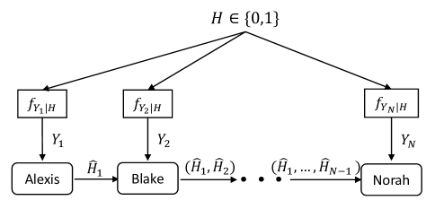
Figure 1: A cascading decision making model with N𝑁N agents.

Consider an N𝑁N-agent cascading decision making problem, as illustrated in Fig. 1. The underlying hypothesis, H{0,1}𝐻01H\in\{0,1\}, is a binary signal with prior H=0=p0𝐻0subscript𝑝0\mathbb{P}{H=0}=p_{0} and H=1=1p0𝐻11subscript𝑝0\mathbb{P}{H=1}=1-p_{0}. There are N𝑁N agents that sequentially detect the state in a predetermined order. The n𝑛nth agent has a private signal Ynsubscript𝑌𝑛Y_{n} generated according to the likelihood fYn|Hsubscript𝑓conditionalsubscript𝑌𝑛𝐻f_{Y_{n}|H}, which is not necessarily identical for all n𝑛n. Let the decision made by the n𝑛nth agent be H^nsubscript^𝐻𝑛\widehat{H}_{n}. In addition to the private signal, the n𝑛nth agent also observes the decisions made by preceding agents, {H^1,,H^n1}subscript^𝐻1subscript^𝐻𝑛1\{\widehat{H}_{1},\ldots,\widehat{H}_{n-1}\}, to make a decision H^nsubscript^𝐻𝑛\widehat{H}_{n}.

However, the n𝑛nth agent believes the prior probability of the null hypothesis is qn(0,1)subscript𝑞𝑛01q_{n}\in(0,1) as against the true prior probability p0subscript𝑝0p_{0}. We call this the belief of the agent in order to distinguish it from the prior. Agent n𝑛n is also aware of her own likelihood fYn|Hsubscript𝑓conditionalsubscript𝑌𝑛𝐻f_{Y_{n}|H} that defines her private signal. However, she also perceives the likelihoods and beliefs of the other agents to be the same as hers, i.e., she thinks fYj|H=fYn|H,qj=qnformulae-sequencesubscript𝑓conditionalsubscript𝑌𝑗𝐻subscript𝑓conditionalsubscript𝑌𝑛𝐻subscript𝑞𝑗subscript𝑞𝑛f_{Y_{j}|H}=f_{Y_{n}|H},q_{j}=q_{n} for all jn𝑗𝑛j\neq n, even though they could be different and unknown to her. We assume that the likelihood ratio of each agent is an increasing function in y𝑦y,222This property is particularly useful in uniformly most powerful (UMP) tests. i.e., for all agents

n(y):=fYn|H(y|1)fYn|H(y|0)assignsubscript𝑛𝑦subscript𝑓conditionalsubscript𝑌𝑛𝐻conditional𝑦1subscript𝑓conditionalsubscript𝑌𝑛𝐻conditional𝑦0\displaystyle\mathcal{L}_{n}(y):=\frac{f_{Y_{n}|H}(y|1)}{f_{Y_{n}|H}(y|0)}

is an increasing function of y𝑦y.

Several numerical examples are given for private signals defined with independent additive Gaussian noise. The desired monotonicity also holds for many non-additive models, such as exponential distribution with mean H1superscript𝐻1H^{-1}, H+𝐻subscriptH\in\mathbb{R}_{+}, binomial distribution with success probability H[0,1]𝐻01H\in[0,1], and Poisson distribution with rate H+𝐻subscriptH\in\mathbb{R}_{+} are members of such family, where H𝐻H could take two values.

Our performance analysis focuses on the last agent (N𝑁Nth agent, Norah) and her decision ̵̂H^Nsubscript^𝐻𝑁\widehat{H}_{N}. Upon observing her private signal YNsubscript𝑌𝑁Y_{N} and the (N1)𝑁1(N-1) preceding decisions, she determines her decision rule. The relative importance of correct decisions and errors can be abstracted as a cost function. For simplicity, we assume correct decisions have zero cost and use the shorthand notations c10=c(1,0)subscript𝑐10𝑐10c_{10}=c(1,0) as the cost for false alarm or Type I error (choosing ̵̂H^=1^𝐻1\widehat{H}=1 when H=0𝐻0H=0), and c01=c(0,1)subscript𝑐01𝑐01c_{01}=c(0,1) as the cost for missed detection or Type II error (choosing H^=0^𝐻0\widehat{H}=0 when H=1𝐻1H=1). In addition, we assume that agents have the same costs; they are a team in the sense of Radner [33]. Then the Bayes risk is

RN=c10p0pH^N|H(1|0)+c01(1p0)pH^N|H(0|1).subscript𝑅𝑁subscript𝑐10subscript𝑝0subscript𝑝conditionalsubscript^𝐻𝑁𝐻conditional10subscript𝑐011subscript𝑝0subscript𝑝conditionalsubscript^𝐻𝑁𝐻conditional01\displaystyle R_{N}=c_{10}p_{0}p_{\widehat{H}_{N}|H}(1|0)+c_{01}(1-p_{0})p_{\widehat{H}_{N}|H}(0|1). (1)

As H^nsubscript^𝐻𝑛\widehat{H}_{n} depends on the previous decisions, the computation of (1) also depends on (H^1,,H^N1)subscript^𝐻1subscript^𝐻𝑁1(\widehat{H}_{1},\ldots,\widehat{H}_{N-1}), and the Bayes risk can be expanded as

RNsubscript𝑅𝑁\displaystyle R_{N} =h^1,,h^N1c10p0pH^N,H^N1,,H^1|H(1,h^N1,,h^1|0)absentsubscriptsubscript^1subscript^𝑁1subscript𝑐10subscript𝑝0subscript𝑝subscript^𝐻𝑁subscript^𝐻𝑁1conditionalsubscript^𝐻1𝐻1subscript^𝑁1conditionalsubscript^10\displaystyle=\sum_{\widehat{h}_{1},\ldots,\widehat{h}_{N-1}}c_{10}p_{0}p_{\widehat{H}_{N},\widehat{H}_{N-1},\ldots,\widehat{H}_{1}|H}(1,\widehat{h}_{N-1},\ldots,\widehat{h}_{1}|0)
+c01(1p0)pH^N,H^N1,,H^1|H(0,h^N1,,h^1|1).subscript𝑐011subscript𝑝0subscript𝑝subscript^𝐻𝑁subscript^𝐻𝑁1conditionalsubscript^𝐻1𝐻0subscript^𝑁1conditionalsubscript^11\displaystyle+c_{01}(1-p_{0})p_{\widehat{H}_{N},\widehat{H}_{N-1},\ldots,\widehat{H}_{1}|H}(0,\widehat{h}_{N-1},\ldots,\widehat{h}_{1}|1). (2)

We determine the optimal set of beliefs of the agents {qn}n=1Nsuperscriptsubscriptsuperscriptsubscript𝑞𝑛𝑛1𝑁\{q_{n}^{*}\}_{n=1}^{N} that minimize (2).

In our model, the n𝑛nth agent minimizes her perceived Bayes risk, which is the Bayes risk with prior probability p0subscript𝑝0p_{0} replaced by her belief qnsubscript𝑞𝑛q_{n}. In other words, for all n=1,,N𝑛1𝑁n=1,\ldots,N, the n𝑛nth agent adopts the decision rule that minimizes her perceived Bayes risk Rnsubscript𝑅𝑛R_{n}, and her decision is revealed to other agents as a public signal. The decisions {H^1,,H^n1}subscript^𝐻1subscript^𝐻𝑛1\{\widehat{H}_{1},\ldots,\widehat{H}_{n-1}\} of the earlier-acting agents reveal information about H𝐻H and thus should be incorporated into the decision-making process by agent n𝑛n. As mentioned earlier, since she believes qnsubscript𝑞𝑛q_{n} is the true prior, she aggregates information under the assumption that q1=q2==qnsubscript𝑞1subscript𝑞2subscript𝑞𝑛q_{1}=q_{2}=\cdots=q_{n}.

It is important to note that every agent is selfish and rational; the agents do not adjust their decision rules for Norah’s sake. The novelty in the model (and hence in the conclusions) comes from agent n𝑛n having the limitation of using a private initial belief qnsubscript𝑞𝑛q_{n} in place of the true prior probability p0subscript𝑝0p_{0}.

II-A Prospect Theory

Let us also formally introduce the Prelec reweighting function from cumulative prospect-theoretic models of human behavior. It spans a family of open- and closed-minded beliefs (will be clarified later) and thus the optimal beliefs that emerge in following sections could be approximated by a function in the Prelec family.

Definition 1 ([38])

For α,β>0𝛼𝛽0\alpha,\beta>0, the Prelec reweighting function w:[0,1][0,1]:𝑤maps-to0101w:[0,1]\mapsto[0,1] is

w(p;α,β)=exp(β(logp)α).𝑤𝑝𝛼𝛽𝛽superscript𝑝𝛼\displaystyle w(p;\alpha,\beta)=\exp(-\beta(-\log p)^{\alpha}).

The function satisfies several properties such as:

  1. 1.

    w(p;α,β)𝑤𝑝𝛼𝛽w(p;\alpha,\beta) is strictly increasing;

  2. 2.

    has a unique fixed point w(p;α,β)=p𝑤𝑝𝛼𝛽𝑝w(p;\alpha,\beta)=p at p=exp(exp(logβ/(1α)))superscript𝑝𝛽1𝛼p^{*}=\exp(-\exp(\log\beta/(1-\alpha))); and

  3. 3.

    spans a class of open-minded beliefs when α<1𝛼1\alpha<1, i.e., overweights (underweights) small (high) probability, and vice versa when α>1𝛼1\alpha>1.

A more generic form, termed composite Prelec weighting function, has been defined in [39].

II-B Notations

Throughout the paper, we use f𝑓f for continuous probability density functions and p𝑝p for discrete probability mass functions. All logarithms are natural logarithms. We use 𝒩(μ,σ2)𝒩𝜇superscript𝜎2\mathcal{N}(\mu,\sigma^{2}) to denote a Gaussian distribution with mean μ𝜇\mu and variance σ2superscript𝜎2\sigma^{2}, and ϕ(x;μ,σ2)italic-ϕ𝑥𝜇superscript𝜎2\phi(x;\mu,\sigma^{2}) to denote its density function, i.e.,

ϕ(x;μ,σ2)=12πσ2e(xμ)22σ2.italic-ϕ𝑥𝜇superscript𝜎212𝜋superscript𝜎2superscript𝑒superscript𝑥𝜇22superscript𝜎2\displaystyle\phi(x;\mu,\sigma^{2})=\frac{1}{\sqrt{2\pi\sigma^{2}}}e^{-\frac{(x-\mu)^{2}}{2\sigma^{2}}}.

Also in the case of the standard Gaussian, ϕ(x):=ϕ(x;0,1)assignitalic-ϕ𝑥italic-ϕ𝑥01\phi(x):=\phi(x;0,1) for simplicity. Q(x)𝑄𝑥Q(x) is defined as the complementary cumulative distribution function of the standard Gaussian,

Q(x)=xϕ(t)𝑑t.𝑄𝑥superscriptsubscript𝑥italic-ϕ𝑡differential-d𝑡\displaystyle Q(x)=\int_{x}^{\infty}\phi(t)dt.

III Belief Update and Sequential Decision Making

Our model assumes unbounded private signals. Thus, unlike in [5, 6], it is always possible that a subsequent agent may not follow previous decisions; that is, herding happens with arbitrarily low probability. We now discuss using both a decision history and private signals for Bayesian binary hypothesis testing. The decision rule can be interpreted as each agent updating her posterior belief based on the decision history and then applying a likelihood ratio test to her private signal.

III-A Alexis, the First Agent

Since Alexis has no prior decision history, she follows usual binary hypothesis testing. She uses the following likelihood ratio test with her initial belief q1subscript𝑞1q_{1}, with ties broken arbitrarily:

1(y1)=fY1|H(y1|1)fY1|H(y1|0)H^1=0H^1=1c10q1c01(1q1).subscript1subscript𝑦1subscript𝑓conditionalsubscript𝑌1𝐻conditionalsubscript𝑦11subscript𝑓conditionalsubscript𝑌1𝐻conditionalsubscript𝑦10subscript^𝐻10subscript^𝐻11greater-than-or-less-thansubscript𝑐10subscript𝑞1subscript𝑐011subscript𝑞1\displaystyle\mathcal{L}_{1}(y_{1})=\frac{f_{Y_{1}|H}(y_{1}|1)}{f_{Y_{1}|H}(y_{1}|0)}\underset{\widehat{H}_{1}=0}{\overset{\widehat{H}_{1}=1}{\gtrless}}\frac{c_{10}q_{1}}{c_{01}(1-q_{1})}. (3)

Since we assume the likelihood ratio is increasing in y1subscript𝑦1y_{1}, the rule simplifies to comparing the private signal with an appropriate decision threshold:

y1H^1=0H^1=1λ1(q1),subscript𝑦1subscript^𝐻10subscript^𝐻11greater-than-or-less-thansubscript𝜆1subscript𝑞1\displaystyle y_{1}\underset{\widehat{H}_{1}=0}{\overset{\widehat{H}_{1}=1}{\gtrless}}\lambda_{1}(q_{1}), (4)

where λi(q)subscript𝜆𝑖𝑞\lambda_{i}(q) denotes the decision threshold λ𝜆\lambda that satisfies

i(λ)=fYi|H(λ|1)fYi|H(λ|0)=c10qc01(1q).subscript𝑖𝜆subscript𝑓conditionalsubscript𝑌𝑖𝐻conditional𝜆1subscript𝑓conditionalsubscript𝑌𝑖𝐻conditional𝜆0subscript𝑐10𝑞subscript𝑐011𝑞\displaystyle\mathcal{L}_{i}(\lambda)=\frac{f_{Y_{i}|H}(\lambda|1)}{f_{Y_{i}|H}(\lambda|0)}=\frac{c_{10}q}{c_{01}(1-q)}. (5)

III-B Blake, the Second Agent

Blake observes Alexis’s decision H^1=h^1subscript^𝐻1subscript^1\widehat{H}_{1}=\widehat{h}_{1} and evaluates the likelihood ratio for (H^1,Y2)subscript^𝐻1subscript𝑌2(\widehat{H}_{1},Y_{2}), using his initial belief q2subscript𝑞2q_{2} as

fY2,H^1|H(y2,h^1|1)fY2,H^1|H(y2,h^1|0)H^2=0H^2=1c10q2c01(1q2).subscript𝑓subscript𝑌2conditionalsubscript^𝐻1𝐻subscript𝑦2conditionalsubscript^11subscript𝑓subscript𝑌2conditionalsubscript^𝐻1𝐻subscript𝑦2conditionalsubscript^10subscript^𝐻20subscript^𝐻21greater-than-or-less-thansubscript𝑐10subscript𝑞2subscript𝑐011subscript𝑞2\displaystyle\frac{f_{Y_{2},\widehat{H}_{1}|H}(y_{2},\widehat{h}_{1}|1)}{f_{Y_{2},\widehat{H}_{1}|H}(y_{2},\widehat{h}_{1}|0)}\underset{\widehat{H}_{2}=0}{\overset{\widehat{H}_{2}=1}{\gtrless}}\frac{c_{10}q_{2}}{c_{01}(1-q_{2})}. (6)

The private signals Y1subscript𝑌1Y_{1} and Y2subscript𝑌2Y_{2} are independent conditioned on H𝐻H, so H^1subscript^𝐻1\widehat{H}_{1} and Y2subscript𝑌2Y_{2} are also independent conditioned on H𝐻H. Hence, the left side of (6) is

fY2,H^1|H(y2,h^1|h)=fY2|H(y2|h)pH^1|H(h^1|h).subscript𝑓subscript𝑌2conditionalsubscript^𝐻1𝐻subscript𝑦2conditionalsubscript^1subscript𝑓conditionalsubscript𝑌2𝐻conditionalsubscript𝑦2subscript𝑝conditionalsubscript^𝐻1𝐻conditionalsubscript^1\displaystyle f_{Y_{2},\widehat{H}_{1}|H}(y_{2},\widehat{h}_{1}|h)=f_{Y_{2}|H}(y_{2}|h)p_{\widehat{H}_{1}|H}(\widehat{h}_{1}|h).

So we can rewrite (6) as333The subscript [2]delimited-[]2[2] in the term pH^1|H(h^1|h)[2]subscript𝑝conditionalsubscript^𝐻1𝐻subscriptconditionalsubscript^1delimited-[]2p_{\widehat{H}_{1}|H}(\widehat{h}_{1}|h)_{[2]} indicates the value of pH^1|H(h^1|h)subscript𝑝conditionalsubscript^𝐻1𝐻conditionalsubscript^1p_{\widehat{H}_{1}|H}(\widehat{h}_{1}|h) that Blake (the second agent) thinks. We specify this because Blake does not know Alexis’s belief q1subscript𝑞1q_{1}. Thus, he interprets her decision based on his belief q2subscript𝑞2q_{2}. The value is different from the true value of pH^1|H(h^1|h)=pH^1|H(h^1|h)[1]subscript𝑝conditionalsubscript^𝐻1𝐻conditionalsubscript^1subscript𝑝conditionalsubscript^𝐻1𝐻subscriptconditionalsubscript^1delimited-[]1p_{\widehat{H}_{1}|H}(\widehat{h}_{1}|h)=p_{\widehat{H}_{1}|H}(\widehat{h}_{1}|h)_{[1]}. Of course, it will also be different from what Chuck, the third agent, perceives, which is denoted by pH^1|H(h^1|h)[3]subscript𝑝conditionalsubscript^𝐻1𝐻subscriptconditionalsubscript^1delimited-[]3p_{\widehat{H}_{1}|H}(\widehat{h}_{1}|h)_{[3]}. This will be explained in the next subsection.

fY2|H(y2|1)fY2|H(y2|0)H^2=0H^2=1c10q2c01(1q2)pH^1|H(h^1|0)[2]pH^1|H(h^1|1)[2].subscript𝑓conditionalsubscript𝑌2𝐻conditionalsubscript𝑦21subscript𝑓conditionalsubscript𝑌2𝐻conditionalsubscript𝑦20subscript^𝐻20subscript^𝐻21greater-than-or-less-thansubscript𝑐10subscript𝑞2subscript𝑐011subscript𝑞2subscript𝑝conditionalsubscript^𝐻1𝐻subscriptconditionalsubscript^10delimited-[]2subscript𝑝conditionalsubscript^𝐻1𝐻subscriptconditionalsubscript^11delimited-[]2\displaystyle\frac{f_{Y_{2}|H}(y_{2}|1)}{f_{Y_{2}|H}(y_{2}|0)}\underset{\widehat{H}_{2}=0}{\overset{\widehat{H}_{2}=1}{\gtrless}}\frac{c_{10}q_{2}}{c_{01}(1-q_{2})}\frac{p_{\widehat{H}_{1}|H}(\widehat{h}_{1}|0)_{[2]}}{p_{\widehat{H}_{1}|H}(\widehat{h}_{1}|1)_{[2]}}. (7)

The likelihood ratio test (7) can be interpreted as Blake updating his initial belief upon observing Alexis’s decision H^1subscript^𝐻1\widehat{H}_{1}. Combined with q2subscript𝑞2q_{2}, his initial belief is updated according to pH^1|H(h^1|h)[2]subscript𝑝conditionalsubscript^𝐻1𝐻subscriptconditionalsubscript^1delimited-[]2p_{\widehat{H}_{1}|H}(\widehat{h}_{1}|h)_{[2]}, from q2subscript𝑞2q_{2} to q2h^1superscriptsubscript𝑞2subscript^1q_{2}^{\widehat{h}_{1}}:

q2h^11q2h^1=q21q2pH^1|H(h^1|0)[2]pH^1|H(h^1|1)[2].superscriptsubscript𝑞2subscript^11superscriptsubscript𝑞2subscript^1subscript𝑞21subscript𝑞2subscript𝑝conditionalsubscript^𝐻1𝐻subscriptconditionalsubscript^10delimited-[]2subscript𝑝conditionalsubscript^𝐻1𝐻subscriptconditionalsubscript^11delimited-[]2\displaystyle\frac{q_{2}^{\widehat{h}_{1}}}{1-q_{2}^{\widehat{h}_{1}}}=\frac{q_{2}}{1-q_{2}}\frac{p_{\widehat{H}_{1}|H}(\widehat{h}_{1}|0)_{[2]}}{p_{\widehat{H}_{1}|H}(\widehat{h}_{1}|1)_{[2]}}. (8)

The posterior belief is

q2h^1superscriptsubscript𝑞2subscript^1\displaystyle q_{2}^{\widehat{h}_{1}} =q2pH^1|H(h^1|0)[2]q2pH^1|H(h^1|0)[2]+(1q2)pH^1|H(h^1|1)[2]absentsubscript𝑞2subscript𝑝conditionalsubscript^𝐻1𝐻subscriptconditionalsubscript^10delimited-[]2subscript𝑞2subscript𝑝conditionalsubscript^𝐻1𝐻subscriptconditionalsubscript^10delimited-[]21subscript𝑞2subscript𝑝conditionalsubscript^𝐻1𝐻subscriptconditionalsubscript^11delimited-[]2\displaystyle=\frac{q_{2}p_{\widehat{H}_{1}|H}(\widehat{h}_{1}|0)_{[2]}}{q_{2}p_{\widehat{H}_{1}|H}(\widehat{h}_{1}|0)_{[2]}+(1-q_{2})p_{\widehat{H}_{1}|H}(\widehat{h}_{1}|1)_{[2]}} (9)
=pH^1,H(h^1,0)[2]pH^1,H(h^1,0)[2]+pH^1,H(h^1,1)[2]absentsubscript𝑝subscript^𝐻1𝐻subscriptsubscript^10delimited-[]2subscript𝑝subscript^𝐻1𝐻subscriptsubscript^10delimited-[]2subscript𝑝subscript^𝐻1𝐻subscriptsubscript^11delimited-[]2\displaystyle=\frac{p_{\widehat{H}_{1},H}(\widehat{h}_{1},0)_{[2]}}{p_{\widehat{H}_{1},H}(\widehat{h}_{1},0)_{[2]}+p_{\widehat{H}_{1},H}(\widehat{h}_{1},1)_{[2]}}
=pH|H^1(0|h^1)[2].absentsubscript𝑝conditional𝐻subscript^𝐻1subscriptconditional0subscript^1delimited-[]2\displaystyle=p_{H|\widehat{H}_{1}}(0|\widehat{h}_{1})_{[2]}.

It should be noted that the true pH^1|H(h^1|h)subscript𝑝conditionalsubscript^𝐻1𝐻conditionalsubscript^1p_{\widehat{H}_{1}|H}(\widehat{h}_{1}|h) is given by

pH^1|H(0|h)subscript𝑝conditionalsubscript^𝐻1𝐻conditional0\displaystyle p_{\widehat{H}_{1}|H}(0|h) =pH^1|H(0|h)[1]=Y1λ1(q1)|H=habsentsubscript𝑝conditionalsubscript^𝐻1𝐻subscriptconditional0delimited-[]1subscript𝑌1conditionalsubscript𝜆1subscript𝑞1𝐻\displaystyle=p_{\widehat{H}_{1}|H}(0|h)_{[1]}=\mathbb{P}{Y_{1}\leq\lambda_{1}(q_{1})|H=h}
=λ1(q1)fY1|H(y|h)𝑑y,absentsuperscriptsubscriptsubscript𝜆1subscript𝑞1subscript𝑓conditionalsubscript𝑌1𝐻conditional𝑦differential-d𝑦\displaystyle=\int_{-\infty}^{\lambda_{1}(q_{1})}f_{Y_{1}|H}(y|h)dy,
pH^1|H(1|h)subscript𝑝conditionalsubscript^𝐻1𝐻conditional1\displaystyle p_{\widehat{H}_{1}|H}(1|h) =λ1(q1)fY1|H(y|h)𝑑y.absentsuperscriptsubscriptsubscript𝜆1subscript𝑞1subscript𝑓conditionalsubscript𝑌1𝐻conditional𝑦differential-d𝑦\displaystyle=\int_{\lambda_{1}(q_{1})}^{\infty}f_{Y_{1}|H}(y|h)dy.

But Blake evaluates Alexis’s decision H^1subscript^𝐻1\widehat{H}_{1} as if it were made based on q2subscript𝑞2q_{2} and the likelihood fY2|H()subscript𝑓conditionalsubscript𝑌2𝐻f_{Y_{2}|H}(\cdot), as against q1,fY1|H()subscript𝑞1subscript𝑓conditionalsubscript𝑌1𝐻q_{1},f_{Y_{1}|H}(\cdot) respectively. Thus the probability pH^1|H(h^1|h)subscript𝑝conditionalsubscript^𝐻1𝐻conditionalsubscript^1p_{\widehat{H}_{1}|H}(\widehat{h}_{1}|h) is computed based on λ2(q2)subscript𝜆2subscript𝑞2\lambda_{2}(q_{2}), instead of λ1(q2)subscript𝜆1subscript𝑞2\lambda_{1}(q_{2}):

pH^1|H(0|h)[2]subscript𝑝conditionalsubscript^𝐻1𝐻subscriptconditional0delimited-[]2\displaystyle p_{\widehat{H}_{1}|H}(0|h)_{[2]} =λ2(q2)fY2|H(y|h)𝑑y,absentsuperscriptsubscriptsubscript𝜆2subscript𝑞2subscript𝑓conditionalsubscript𝑌2𝐻conditional𝑦differential-d𝑦\displaystyle=\int_{-\infty}^{\lambda_{2}(q_{2})}f_{Y_{2}|H}(y|h)dy, (10a)
pH^1|H(1|h)[2]subscript𝑝conditionalsubscript^𝐻1𝐻subscriptconditional1delimited-[]2\displaystyle p_{\widehat{H}_{1}|H}(1|h)_{[2]} =λ2(q2)fY2|H(y|h)𝑑y.absentsuperscriptsubscriptsubscript𝜆2subscript𝑞2subscript𝑓conditionalsubscript𝑌2𝐻conditional𝑦differential-d𝑦\displaystyle=\int_{\lambda_{2}(q_{2})}^{\infty}f_{Y_{2}|H}(y|h)dy. (10b)

An interesting observation is that Alexis’s belief q1subscript𝑞1q_{1} does not affect Blake’s belief update as observed in (9) and (10). That is, for any belief q1subscript𝑞1q_{1} that Alexis might hold, Blake, who does not know this belief, presumes that the conditional probabilities are computed according to (10) and updates his belief as in (9) which depends only on Blake’s initial belief and Alexis’s decision.

However, Alexis’s initial belief implicitly affects Blake’s performance since her biased belief changes the resulting decisions whose probabilities are embedded in the probability of Blake’s decision:

pH^2|H(h^2|h)subscript𝑝conditionalsubscript^𝐻2𝐻conditionalsubscript^2\displaystyle p_{\widehat{H}_{2}|H}(\widehat{h}_{2}|h) =h^1{0,1}pH^2,H^1|H(h^2,h^1|h)absentsubscriptsubscript^101subscript𝑝subscript^𝐻2conditionalsubscript^𝐻1𝐻subscript^2conditionalsubscript^1\displaystyle=\sum_{\widehat{h}_{1}\in\{0,1\}}p_{\widehat{H}_{2},\widehat{H}_{1}|H}(\widehat{h}_{2},\widehat{h}_{1}|h)
=pH^2|H^1,H(h^2|0,h)[2]×pH^1|H(0|h)[1]absentsubscript𝑝conditionalsubscript^𝐻2subscript^𝐻1𝐻subscriptconditionalsubscript^20delimited-[]2subscript𝑝conditionalsubscript^𝐻1𝐻subscriptconditional0delimited-[]1\displaystyle=p_{\widehat{H}_{2}|\widehat{H}_{1},H}(\widehat{h}_{2}|0,h)_{[2]}\times p_{\widehat{H}_{1}|H}(0|h)_{[1]}
+pH^2|H^1,H(h^2|1,h)[2]×pH^1|H(1|h)[1].subscript𝑝conditionalsubscript^𝐻2subscript^𝐻1𝐻subscriptconditionalsubscript^21delimited-[]2subscript𝑝conditionalsubscript^𝐻1𝐻subscriptconditional1delimited-[]1\displaystyle~{}~{}~{}+p_{\widehat{H}_{2}|\widehat{H}_{1},H}(\widehat{h}_{2}|1,h)_{[2]}\times p_{\widehat{H}_{1}|H}(1|h)_{[1]}.

Thus, Alexis’s biased belief changes the probability of not only her decision but also of Blake’s decision.

III-C Chuck, the Third Agent

Chuck’s detection process is similar to Blake’s. He observes both Alexis’s and Blake’s decisions and also updates his initial belief q3subscript𝑞3q_{3} like in (8):

q3h^1,h^21q3h^1,h^2superscriptsubscript𝑞3subscript^1subscript^21superscriptsubscript𝑞3subscript^1subscript^2\displaystyle\frac{q_{3}^{\widehat{h}_{1},\widehat{h}_{2}}}{1-q_{3}^{\widehat{h}_{1},\widehat{h}_{2}}} =q31q3pH^2,H^1|H(h^2,h^1|0)[3]pH^2,H^1|H(h^2,h^1|1)[3]absentsubscript𝑞31subscript𝑞3subscript𝑝subscript^𝐻2conditionalsubscript^𝐻1𝐻subscriptsubscript^2conditionalsubscript^10delimited-[]3subscript𝑝subscript^𝐻2conditionalsubscript^𝐻1𝐻subscriptsubscript^2conditionalsubscript^11delimited-[]3\displaystyle=\frac{q_{3}}{1-q_{3}}\frac{p_{\widehat{H}_{2},\widehat{H}_{1}|H}(\widehat{h}_{2},\widehat{h}_{1}|0)_{[3]}}{p_{\widehat{H}_{2},\widehat{H}_{1}|H}(\widehat{h}_{2},\widehat{h}_{1}|1)_{[3]}} (11)
=(q31q3pH^1|H(h^1|0)[3]pH^1|H(h^1|1)[3])pH^2|H^1,H(h^2|h^1,0)[3]pH^2|H^1,H(h^2|h^1,1)[3].absentsubscript𝑞31subscript𝑞3subscript𝑝conditionalsubscript^𝐻1𝐻subscriptconditionalsubscript^10delimited-[]3subscript𝑝conditionalsubscript^𝐻1𝐻subscriptconditionalsubscript^11delimited-[]3subscript𝑝conditionalsubscript^𝐻2subscript^𝐻1𝐻subscriptconditionalsubscript^2subscript^10delimited-[]3subscript𝑝conditionalsubscript^𝐻2subscript^𝐻1𝐻subscriptconditionalsubscript^2subscript^11delimited-[]3\displaystyle=\left(\frac{q_{3}}{1-q_{3}}\frac{p_{\widehat{H}_{1}|H}(\widehat{h}_{1}|0)_{[3]}}{p_{\widehat{H}_{1}|H}(\widehat{h}_{1}|1)_{[3]}}\right)\frac{p_{\widehat{H}_{2}|\widehat{H}_{1},H}(\widehat{h}_{2}|\widehat{h}_{1},0)_{[3]}}{p_{\widehat{H}_{2}|\widehat{H}_{1},H}(\widehat{h}_{2}|\widehat{h}_{1},1)_{[3]}}.

Note that H^1subscript^𝐻1\widehat{H}_{1} and H^2subscript^𝐻2\widehat{H}_{2} are not conditionally independent given H𝐻H as Blake’s decision H^2subscript^𝐻2\widehat{H}_{2} depends on Alexis’s decision H^1subscript^𝐻1\widehat{H}_{1}.

Chuck’s belief update can be understood as a two-step process. The first step is to update his belief according to Alexis’s decision:

q3h^11q3h^1=q31q3pH^1|H(h^1|0)[3]pH^1|H(h^1|1)[3].superscriptsubscript𝑞3subscript^11superscriptsubscript𝑞3subscript^1subscript𝑞31subscript𝑞3subscript𝑝conditionalsubscript^𝐻1𝐻subscriptconditionalsubscript^10delimited-[]3subscript𝑝conditionalsubscript^𝐻1𝐻subscriptconditionalsubscript^11delimited-[]3\displaystyle\frac{q_{3}^{\widehat{h}_{1}}}{1-q_{3}^{\widehat{h}_{1}}}=\frac{q_{3}}{1-q_{3}}\frac{p_{\widehat{H}_{1}|H}(\widehat{h}_{1}|0)_{[3]}}{p_{\widehat{H}_{1}|H}(\widehat{h}_{1}|1)_{[3]}}. (12)

The second step is to update it from q3h^1superscriptsubscript𝑞3subscript^1q_{3}^{\widehat{h}_{1}} based on Blake’s decision:

q3h^1,h^21q3h^1,h^2=q3h^11q3h^1pH^2|H^1,H(h^2|h^1,0)[3]pH^2|H^1,H(h^2|h^1,1)[3].superscriptsubscript𝑞3subscript^1subscript^21superscriptsubscript𝑞3subscript^1subscript^2superscriptsubscript𝑞3subscript^11superscriptsubscript𝑞3subscript^1subscript𝑝conditionalsubscript^𝐻2subscript^𝐻1𝐻subscriptconditionalsubscript^2subscript^10delimited-[]3subscript𝑝conditionalsubscript^𝐻2subscript^𝐻1𝐻subscriptconditionalsubscript^2subscript^11delimited-[]3\displaystyle\frac{q_{3}^{\widehat{h}_{1},\widehat{h}_{2}}}{1-q_{3}^{\widehat{h}_{1},\widehat{h}_{2}}}=\frac{q_{3}^{\widehat{h}_{1}}}{1-q_{3}^{\widehat{h}_{1}}}\frac{p_{\widehat{H}_{2}|\widehat{H}_{1},H}(\widehat{h}_{2}|\widehat{h}_{1},0)_{[3]}}{p_{\widehat{H}_{2}|\widehat{H}_{1},H}(\widehat{h}_{2}|\widehat{h}_{1},1)_{[3]}}. (13)

Again, Chuck is not aware of neither Alexis’s nor Blake’s initial beliefs or likelihoods. Thus, Chuck computes all probabilities based on his own belief q3subscript𝑞3q_{3} and likelihood fY3|Hsubscript𝑓conditionalsubscript𝑌3𝐻f_{Y_{3}|H}, which is indicated by the subscript [3]delimited-[]3[3] in (12) and (13).

Details of computations of (12) and (13) are as follows:

pH^1|H(0|h)[3]subscript𝑝conditionalsubscript^𝐻1𝐻subscriptconditional0delimited-[]3\displaystyle p_{\widehat{H}_{1}|H}(0|h)_{[3]} =λ3(q3)fY3|H(y|h)𝑑y,absentsuperscriptsubscriptsubscript𝜆3subscript𝑞3subscript𝑓conditionalsubscript𝑌3𝐻conditional𝑦differential-d𝑦\displaystyle=\int_{-\infty}^{\lambda_{3}(q_{3})}f_{Y_{3}|H}(y|h)dy,
pH^1|H(1|h)[3]subscript𝑝conditionalsubscript^𝐻1𝐻subscriptconditional1delimited-[]3\displaystyle p_{\widehat{H}_{1}|H}(1|h)_{[3]} =λ3(q3)fY3|H(y|h)𝑑y.absentsuperscriptsubscriptsubscript𝜆3subscript𝑞3subscript𝑓conditionalsubscript𝑌3𝐻conditional𝑦differential-d𝑦\displaystyle=\int_{\lambda_{3}(q_{3})}^{\infty}f_{Y_{3}|H}(y|h)dy.

Similar to Blake (8), Chuck computes q3h^1superscriptsubscript𝑞3subscript^1q_{3}^{\widehat{h}_{1}} for H^1=0subscript^𝐻10\widehat{H}_{1}=0 and H^1=1subscript^𝐻11\widehat{H}_{1}=1 respectively as:

q30superscriptsubscript𝑞30\displaystyle q_{3}^{0} =q3q3+(1q3)λ3(q3)fY3|H(y|1)𝑑yλ3(q3)fY3|H(y|0)𝑑y,absentsubscript𝑞3subscript𝑞31subscript𝑞3superscriptsubscriptsubscript𝜆3subscript𝑞3subscript𝑓conditionalsubscript𝑌3𝐻conditional𝑦1differential-d𝑦superscriptsubscriptsubscript𝜆3subscript𝑞3subscript𝑓conditionalsubscript𝑌3𝐻conditional𝑦0differential-d𝑦\displaystyle=\frac{q_{3}}{q_{3}+(1-q_{3})\frac{\int_{-\infty}^{\lambda_{3}(q_{3})}f_{Y_{3}|H}(y|1)dy}{\int_{-\infty}^{\lambda_{3}(q_{3})}f_{Y_{3}|H}(y|0)dy}}, (14a)
q31superscriptsubscript𝑞31\displaystyle q_{3}^{1} =q3q3+(1q3)λ3(q3)fY3|H(y|1)𝑑yλ3(q3)fY3|H(y|0)𝑑y.absentsubscript𝑞3subscript𝑞31subscript𝑞3superscriptsubscriptsubscript𝜆3subscript𝑞3subscript𝑓conditionalsubscript𝑌3𝐻conditional𝑦1differential-d𝑦superscriptsubscriptsubscript𝜆3subscript𝑞3subscript𝑓conditionalsubscript𝑌3𝐻conditional𝑦0differential-d𝑦\displaystyle=\frac{q_{3}}{q_{3}+(1-q_{3})\frac{\int_{\lambda_{3}(q_{3})}^{\infty}f_{Y_{3}|H}(y|1)dy}{\int_{\lambda_{3}(q_{3})}^{\infty}f_{Y_{3}|H}(y|0)dy}}. (14b)

Then,

pH^2|H^1,H(0|h^1,h)[3]subscript𝑝conditionalsubscript^𝐻2subscript^𝐻1𝐻subscriptconditional0subscript^1delimited-[]3\displaystyle p_{\widehat{H}_{2}|\widehat{H}_{1},H}(0|\widehat{h}_{1},h)_{[3]} =λ3(q3h^1)fY3|H(y|h)𝑑y,absentsuperscriptsubscriptsubscript𝜆3superscriptsubscript𝑞3subscript^1subscript𝑓conditionalsubscript𝑌3𝐻conditional𝑦differential-d𝑦\displaystyle=\int_{-\infty}^{\lambda_{3}(q_{3}^{\widehat{h}_{1}})}f_{Y_{3}|H}(y|h)dy, (15a)
pH^2|H^1,H(1|h^1,h)[3]subscript𝑝conditionalsubscript^𝐻2subscript^𝐻1𝐻subscriptconditional1subscript^1delimited-[]3\displaystyle p_{\widehat{H}_{2}|\widehat{H}_{1},H}(1|\widehat{h}_{1},h)_{[3]} =λ3(q3h^1)fY3|H(y|h)𝑑y.absentsuperscriptsubscriptsubscript𝜆3superscriptsubscript𝑞3subscript^1subscript𝑓conditionalsubscript𝑌3𝐻conditional𝑦differential-d𝑦\displaystyle=\int_{\lambda_{3}(q_{3}^{\widehat{h}_{1}})}^{\infty}f_{Y_{3}|H}(y|h)dy. (15b)

Even though the value of h^1subscript^1\widehat{h}_{1} does not appear in (15), it is implicit in q3h^1superscriptsubscript𝑞3subscript^1q_{3}^{\widehat{h}_{1}} and affects the computation results. Chuck’s posterior belief q3h^1,h^2superscriptsubscript𝑞3subscript^1subscript^2q_{3}^{\widehat{h}_{1},\widehat{h}_{2}} is obtained by substituting (14) and (15) in (13).

III-D Norah, the N𝑁Nth Agent

Norah, the N𝑁Nth agent, observes YNsubscript𝑌𝑁Y_{N} and {H^1,,H^N1}subscript^𝐻1subscript^𝐻𝑁1\{\widehat{H}_{1},\ldots,\widehat{H}_{N-1}\}. Paralleling the arguments in the preceding subsections, her initial belief update is a function of qNsubscript𝑞𝑁q_{N} as well as {H^1,,H^N1}subscript^𝐻1subscript^𝐻𝑁1\{\widehat{H}_{1},\ldots,\widehat{H}_{N-1}\}, but not of {q1,,qN1}subscript𝑞1subscript𝑞𝑁1\{q_{1},\ldots,q_{N-1}\}. Generalizing (11), we have

qNh^1,h^N11qNh^1,h^N1superscriptsubscript𝑞𝑁subscript^1subscript^𝑁11superscriptsubscript𝑞𝑁subscript^1subscript^𝑁1\displaystyle\frac{q_{N}^{\widehat{h}_{1},\ldots\widehat{h}_{N-1}}}{1-q_{N}^{\widehat{h}_{1},\ldots\widehat{h}_{N-1}}} =qN1qNpH^1|H(h^1|0)[N]pH^1|H(h^1|1)[N]×\displaystyle=\frac{q_{N}}{1-q_{N}}\frac{p_{\widehat{H}_{1}|H}(\widehat{h}_{1}|0)_{[N]}}{p_{\widehat{H}_{1}|H}(\widehat{h}_{1}|1)_{[N]}}\times (16)
n=2N1pH^n|H^n1,,H^1,H(h^n|h^n1,,h^1,0)[N]pH^n|H^n1,,H^1,H(h^n|h^n1,,h^1,1)[N].superscriptsubscriptproduct𝑛2𝑁1subscript𝑝conditionalsubscript^𝐻𝑛subscript^𝐻𝑛1subscript^𝐻1𝐻subscriptconditionalsubscript^𝑛subscript^𝑛1subscript^10delimited-[]𝑁subscript𝑝conditionalsubscript^𝐻𝑛subscript^𝐻𝑛1subscript^𝐻1𝐻subscriptconditionalsubscript^𝑛subscript^𝑛1subscript^11delimited-[]𝑁\displaystyle\prod_{n=2}^{N-1}\frac{p_{\widehat{H}_{n}|\widehat{H}_{n-1},\ldots,\widehat{H}_{1},H}(\widehat{h}_{n}|\widehat{h}_{n-1},\ldots,\widehat{h}_{1},0)_{[N]}}{p_{\widehat{H}_{n}|\widehat{H}_{n-1},\ldots,\widehat{H}_{1},H}(\widehat{h}_{n}|\widehat{h}_{n-1},\ldots,\widehat{h}_{1},1)_{[N]}}.

Combining all observations, we obtain the following theorem. Define the initial belief update function for N𝑁Nth agent, UNsubscript𝑈𝑁U_{N} as

qNh^1h^N1=UN(qN,h^1,h^2,,h^N1;N).superscriptsubscript𝑞𝑁subscript^1subscript^𝑁1subscript𝑈𝑁subscript𝑞𝑁subscript^1subscript^2subscript^𝑁1𝑁\displaystyle q_{N}^{\widehat{h}_{1}\ldots\widehat{h}_{N-1}}=U_{N}(q_{N},\widehat{h}_{1},\widehat{h}_{2},\ldots,\widehat{h}_{N-1};N).
Theorem 1

The function Un,nNsubscript𝑈𝑛𝑛𝑁U_{n},n\leq N yielding the posterior belief of N𝑁Nth agent has the following recurrence relation:

  • For n=1𝑛1n=1, U1(q;N)=qsubscript𝑈1𝑞𝑁𝑞U_{1}(q;N)=q.

  • For n>1𝑛1n>1,

    Un(q,h^1,,h^n2,0;N)subscript𝑈𝑛𝑞subscript^1subscript^𝑛20𝑁\displaystyle U_{n}(q,\widehat{h}_{1},\ldots,\widehat{h}_{n-2},0;N)
    =q~q~+(1q~)λN(q~)fYN|H(y|1)𝑑yλN(q~)fYN|H(y|0)𝑑y,absent~𝑞~𝑞1~𝑞superscriptsubscriptsubscript𝜆𝑁~𝑞subscript𝑓conditionalsubscript𝑌𝑁𝐻conditional𝑦1differential-d𝑦superscriptsubscriptsubscript𝜆𝑁~𝑞subscript𝑓conditionalsubscript𝑌𝑁𝐻conditional𝑦0differential-d𝑦\displaystyle~{}~{}~{}~{}~{}~{}=\frac{\tilde{q}}{\tilde{q}+(1-\tilde{q})\frac{\int_{-\infty}^{\lambda_{N}(\tilde{q})}f_{Y_{N}|H}(y|1)dy}{\int_{-\infty}^{\lambda_{N}(\tilde{q})}f_{Y_{N}|H}(y|0)dy}}, (17a)
    Un(q,N,h^1,,h^n2,1;N)subscript𝑈𝑛𝑞𝑁subscript^1subscript^𝑛21𝑁\displaystyle U_{n}(q,N,\widehat{h}_{1},\ldots,\widehat{h}_{n-2},1;N)
    =q~q~+(1q~)λN(q~)fYN|H(y|1)𝑑yλN(q~)fYN|H(y|0)𝑑y,absent~𝑞~𝑞1~𝑞superscriptsubscriptsubscript𝜆𝑁~𝑞subscript𝑓conditionalsubscript𝑌𝑁𝐻conditional𝑦1differential-d𝑦superscriptsubscriptsubscript𝜆𝑁~𝑞subscript𝑓conditionalsubscript𝑌𝑁𝐻conditional𝑦0differential-d𝑦\displaystyle~{}~{}~{}~{}~{}~{}=\frac{\tilde{q}}{\tilde{q}+(1-\tilde{q})\frac{\int_{\lambda_{N}(\tilde{q})}^{\infty}f_{Y_{N}|H}(y|1)dy}{\int_{\lambda_{N}(\tilde{q})}^{\infty}f_{Y_{N}|H}(y|0)dy}}, (17b)

    where q~=Un1(q,h^1,,h^n2;N)~𝑞subscript𝑈𝑛1𝑞subscript^1subscript^𝑛2𝑁\tilde{q}=U_{n-1}(q,\widehat{h}_{1},\ldots,\widehat{h}_{n-2};N).

Note that capital N𝑁N in (17a) and (17b) indicate the recursive updates are computed from the value that the N𝑁Nth agent thinks.

Refer to caption
(a) Noise variance σ2=1superscript𝜎21\sigma^{2}=1
Refer to caption
(b) Noise variance σ2=0.25superscript𝜎20.25\sigma^{2}=0.25
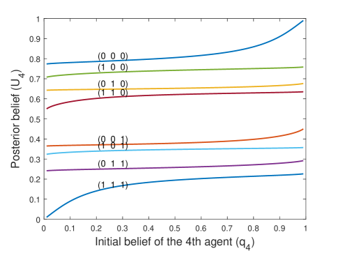
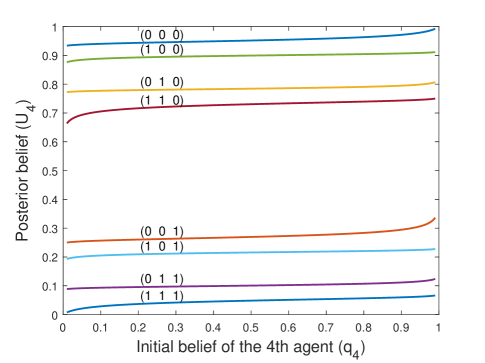
Figure 2: The function U4(q4,h^1,h^2,h^3;4)subscript𝑈4subscript𝑞4subscript^1subscript^2subscript^34U_{4}(q_{4},\widehat{h}_{1},\widehat{h}_{2},\widehat{h}_{3};4)—posterior belief of the fourth agent (q4h^1,h^2,h^3superscriptsubscript𝑞4subscript^1subscript^2subscript^3q_{4}^{\widehat{h}_{1},\widehat{h}_{2},\widehat{h}_{3}})—for each possible combination of Alexis’s, Blake’s, and Chuck’s decisions [h^1,h^2,h^3]subscript^1subscript^2subscript^3[\widehat{h}_{1},\widehat{h}_{2},\widehat{h}_{3}] when c10=c01=1subscript𝑐10subscript𝑐011c_{10}=c_{01}=1 and private signals are distorted by additive Gaussian noise with two noise levels. The posterior belief is mostly dependent on Chuck’s decision; the top four curves are for h^3=0subscript^30\widehat{h}_{3}=0 and the bottom four curves are for h^3=1subscript^31\widehat{h}_{3}=1.

Fig. 2 depicts the function U4(q4,h^1,h^2,h^3;4)subscript𝑈4subscript𝑞4subscript^1subscript^2subscript^34U_{4}(q_{4},\widehat{h}_{1},\widehat{h}_{2},\widehat{h}_{3};4) for N=4𝑁4N=4 for eight possible combinations of Alexis’s, Blake’s, and Chuck’s decisions (h^1,h^2,h^3)subscript^1subscript^2subscript^3(\widehat{h}_{1},\widehat{h}_{2},\widehat{h}_{3}). An interesting property of UNsubscript𝑈𝑁U_{N} is that the posterior belief is much more dependent on the most recent decision h^N1subscript^𝑁1\widehat{h}_{N-1} than on the earlier decisions (h^1,,h^N2)subscript^1subscript^𝑁2(\widehat{h}_{1},\ldots,\widehat{h}_{N-2}). This is because later acting agents consider more previous decisions, and hence more information than the first agents, their decisions should carry more weight. In this sense, we can say that recent decisions give more information than earlier decisions. This is especially the case when the (N1)𝑁1(N-1)th agent has not followed precedent. This is because the N𝑁Nth agent rationally concludes that the (N1)𝑁1(N-1)th agent observed strong evidence to justify a deviation from precedent. For example, if the decision history of the first five agents is (0,0,0,0,1)00001(0,0,0,0,1) then the sixth agent takes the last decision 111 seriously even though the first four agents chose 00. A reversal of an arbitrarily long precedent sequence may occur because we assume unbounded private signals; if private signals are bounded [5, 6], then the influence of the precedent can reach a point where agents cannot receive a signal strong enough to justify a decision running counter to precedent. Another interesting point is that smaller noise variance changes beliefs more. It is clear from (17), but also reasonable that when the variance is smaller, the N𝑁Nth agent trusts and is more inclined towards previous decisions. Note even though the prior updates of Norah in Fig. 2 do not depend on {q1,,qN1}subscript𝑞1subscript𝑞𝑁1\{q_{1},\ldots,q_{N-1}\} and their corresponding likelihoods, the probability of prior decisions depends on them and implicitly, so does Norah’s decision.

As we can see in Fig. 2, the dominant previous decision for agent N𝑁N is the decision of agent (N1)𝑁1(N-1). We can prove that observing the (N1)𝑁1(N-1)th agent’s decision 00 (or decision 111), the N𝑁Nth agent’s posterior belief becomes larger (or smaller), which in turn implies that the decision threshold of N𝑁Nth agent becomes larger (or smaller) so that she is more likely to declare decision 00 (or 111) as well.

Theorem 2

Suppose that noises are independent and additive, and have continuous densities. Fix some prior decisions {h^1,,h^N2}subscript^1subscript^𝑁2\{\widehat{h}_{1},\dots,\widehat{h}_{N-2}\} and let q~N,q~N0,q~N1subscript~𝑞𝑁superscriptsubscript~𝑞𝑁0superscriptsubscript~𝑞𝑁1\tilde{q}_{N},\tilde{q}_{N}^{0},\tilde{q}_{N}^{1} denote the posterior beliefs of the N𝑁Nth agent given the (N2)𝑁2(N-2) decisions only, the (N2)𝑁2(N-2) decisions with h^N1=0subscript^𝑁10\widehat{h}_{N-1}=0, and the (N2)𝑁2(N-2) decisions with h^N1=1subscript^𝑁11\widehat{h}_{N-1}=1. Then,

q~N1<q~N<q~N0.superscriptsubscript~𝑞𝑁1subscript~𝑞𝑁superscriptsubscript~𝑞𝑁0\displaystyle\tilde{q}_{N}^{1}<\tilde{q}_{N}<\tilde{q}_{N}^{0}.
Proof:

We know that q~N,q~N0,q~N1subscript~𝑞𝑁superscriptsubscript~𝑞𝑁0superscriptsubscript~𝑞𝑁1\tilde{q}_{N},\tilde{q}_{N}^{0},\tilde{q}_{N}^{1} differ only by the last multiplicative term of (16). Since q1q𝑞1𝑞\frac{q}{1-q} is monotone increasing, the statement is equivalent to showing:

λN(q~N)fYN|H(y|0)𝑑yλN(q~N)fYN|H(y|1)𝑑y<1<λN(q~N)fYN|H(y|0)𝑑yλN(q~N)fYN|H(y|1)𝑑y.superscriptsubscriptsubscript𝜆𝑁subscript~𝑞𝑁subscript𝑓conditionalsubscript𝑌𝑁𝐻conditional𝑦0differential-d𝑦superscriptsubscriptsubscript𝜆𝑁subscript~𝑞𝑁subscript𝑓conditionalsubscript𝑌𝑁𝐻conditional𝑦1differential-d𝑦1superscriptsubscriptsubscript𝜆𝑁subscript~𝑞𝑁subscript𝑓conditionalsubscript𝑌𝑁𝐻conditional𝑦0differential-d𝑦superscriptsubscriptsubscript𝜆𝑁subscript~𝑞𝑁subscript𝑓conditionalsubscript𝑌𝑁𝐻conditional𝑦1differential-d𝑦\displaystyle\frac{\int_{\lambda_{N}(\tilde{q}_{N})}^{\infty}f_{Y_{N}|H}(y|0)dy}{\int_{\lambda_{N}(\tilde{q}_{N})}^{\infty}f_{Y_{N}|H}(y|1)dy}<1<\frac{\int_{-\infty}^{\lambda_{N}(\tilde{q}_{N})}f_{Y_{N}|H}(y|0)dy}{\int_{-\infty}^{\lambda_{N}(\tilde{q}_{N})}f_{Y_{N}|H}(y|1)dy}.

Since the noise is independent and additive, fYN|H(y|1)=fYN|H(y1|0)subscript𝑓conditionalsubscript𝑌𝑁𝐻conditional𝑦1subscript𝑓conditionalsubscript𝑌𝑁𝐻𝑦conditional10f_{Y_{N}|H}(y|1)=f_{Y_{N}|H}(y-1|0) so the term on the left side

λN(q~N)fYN|H(y|0)𝑑yλN(q~N)fYN|H(y|1)𝑑y=λn(q~N)fYN|H(y|0)𝑑yλN(q~N)1fYN|H(y|0)𝑑ysuperscriptsubscriptsubscript𝜆𝑁subscript~𝑞𝑁subscript𝑓conditionalsubscript𝑌𝑁𝐻conditional𝑦0differential-d𝑦superscriptsubscriptsubscript𝜆𝑁subscript~𝑞𝑁subscript𝑓conditionalsubscript𝑌𝑁𝐻conditional𝑦1differential-d𝑦superscriptsubscriptsubscript𝜆𝑛subscript~𝑞𝑁subscript𝑓conditionalsubscript𝑌𝑁𝐻conditional𝑦0differential-d𝑦superscriptsubscriptsubscript𝜆𝑁subscript~𝑞𝑁1subscript𝑓conditionalsubscript𝑌𝑁𝐻conditional𝑦0differential-d𝑦\displaystyle\frac{\int_{\lambda_{N}(\tilde{q}_{N})}^{\infty}f_{Y_{N}|H}(y|0)dy}{\int_{\lambda_{N}(\tilde{q}_{N})}^{\infty}f_{Y_{N}|H}(y|1)dy}=\frac{\int_{\lambda_{n}(\tilde{q}_{N})}^{\infty}f_{Y_{N}|H}(y|0)dy}{\int_{\lambda_{N}(\tilde{q}_{N})-1}^{\infty}f_{Y_{N}|H}(y|0)dy}
=λN(q~N)fYN|H(y|0)𝑑yλN(q~N)1λN(q~N)fYN|H(y|0)𝑑y+λN(q~N)fYN|H(y|0)𝑑y<1.absentsuperscriptsubscriptsubscript𝜆𝑁subscript~𝑞𝑁subscript𝑓conditionalsubscript𝑌𝑁𝐻conditional𝑦0differential-d𝑦superscriptsubscriptsubscript𝜆𝑁subscript~𝑞𝑁1subscript𝜆𝑁subscript~𝑞𝑁subscript𝑓conditionalsubscript𝑌𝑁𝐻conditional𝑦0differential-d𝑦superscriptsubscriptsubscript𝜆𝑁subscript~𝑞𝑁subscript𝑓conditionalsubscript𝑌𝑁𝐻conditional𝑦0differential-d𝑦1\displaystyle=\frac{\int_{\lambda_{N}(\tilde{q}_{N})}^{\infty}f_{Y_{N}|H}(y|0)dy}{\int_{\lambda_{N}(\tilde{q}_{N})-1}^{\lambda_{N}(\tilde{q}_{N})}f_{Y_{N}|H}(y|0)dy+\int_{\lambda_{N}(\tilde{q}_{N})}^{\infty}f_{Y_{N}|H}(y|0)dy}<1.

The right inequality can be shown similarly. ∎

Considering the complicated relationships that individual decisions have on the evolution of initial beliefs, it is also important to verify if the belief evolution preserves the ordering, given the same set of subsequent decisions. That is, given two beliefs qL<qRsubscript𝑞𝐿subscript𝑞𝑅q_{L}<q_{R} at some point of the recursive update and the same sequence of following d𝑑d decisions, then it is important to characterize the likelihoods for which the the ordering is preserved in the resulting posterior beliefs, given the sequence of decisions, which is described in the following theorem.

Theorem 3

Suppose that noise is independent and additive, and has a continuous density. Consider two beliefs qL<qRsubscript𝑞𝐿subscript𝑞𝑅q_{L}<q_{R}. Then, for any given later-acting decisions d𝑑d, the posterior belief satisfies qLd<qRdsuperscriptsubscript𝑞𝐿𝑑superscriptsubscript𝑞𝑅𝑑q_{L}^{d}<q_{R}^{d} if and only if

g1(q)subscript𝑔1𝑞\displaystyle g_{1}(q) :=q1qλN(q)fYN|H(y|0)𝑑yλN(q)fYN|H(y|1)𝑑y,assignabsent𝑞1𝑞superscriptsubscriptsubscript𝜆𝑁𝑞subscript𝑓conditionalsubscript𝑌𝑁𝐻conditional𝑦0differential-d𝑦superscriptsubscriptsubscript𝜆𝑁𝑞subscript𝑓conditionalsubscript𝑌𝑁𝐻conditional𝑦1differential-d𝑦\displaystyle:=\frac{q}{1-q}\frac{\int_{-\infty}^{\lambda_{N}(q)}f_{Y_{N}|H}(y|0)dy}{\int_{-\infty}^{\lambda_{N}(q)}f_{Y_{N}|H}(y|1)dy}, (18)
g2(q)subscript𝑔2𝑞\displaystyle g_{2}(q) :=q1qλN(q)fYN|H(y|0)𝑑yλN(q)fYN|H(y|1)𝑑yassignabsent𝑞1𝑞superscriptsubscriptsubscript𝜆𝑁𝑞subscript𝑓conditionalsubscript𝑌𝑁𝐻conditional𝑦0differential-d𝑦superscriptsubscriptsubscript𝜆𝑁𝑞subscript𝑓conditionalsubscript𝑌𝑁𝐻conditional𝑦1differential-d𝑦\displaystyle:=\frac{q}{1-q}\frac{\int_{\lambda_{N}(q)}^{\infty}f_{Y_{N}|H}(y|0)dy}{\int_{\lambda_{N}(q)}^{\infty}f_{Y_{N}|H}(y|1)dy} (19)

are both increasing in q𝑞q.

Proof:

Note that once observing decision 00, beliefs are updated as

qL01qL0superscriptsubscript𝑞𝐿01superscriptsubscript𝑞𝐿0\displaystyle\frac{q_{L}^{0}}{1-q_{L}^{0}} =qL1qLλN(qL)fYN|H(y|0)𝑑yλN(qL)fYN|H(y|1)𝑑y,absentsubscript𝑞𝐿1subscript𝑞𝐿superscriptsubscriptsubscript𝜆𝑁subscript𝑞𝐿subscript𝑓conditionalsubscript𝑌𝑁𝐻conditional𝑦0differential-d𝑦superscriptsubscriptsubscript𝜆𝑁subscript𝑞𝐿subscript𝑓conditionalsubscript𝑌𝑁𝐻conditional𝑦1differential-d𝑦\displaystyle=\frac{q_{L}}{1-q_{L}}\frac{\int_{-\infty}^{\lambda_{N}(q_{L})}f_{Y_{N}|H}(y|0)dy}{\int_{-\infty}^{\lambda_{N}(q_{L})}f_{Y_{N}|H}(y|1)dy},
qR01qR0superscriptsubscript𝑞𝑅01superscriptsubscript𝑞𝑅0\displaystyle\frac{q_{R}^{0}}{1-q_{R}^{0}} =qR1qRλN(qR)fYN|H(y|0)𝑑yλN(qR)fYN|H(y|1)𝑑y,absentsubscript𝑞𝑅1subscript𝑞𝑅superscriptsubscriptsubscript𝜆𝑁subscript𝑞𝑅subscript𝑓conditionalsubscript𝑌𝑁𝐻conditional𝑦0differential-d𝑦superscriptsubscriptsubscript𝜆𝑁subscript𝑞𝑅subscript𝑓conditionalsubscript𝑌𝑁𝐻conditional𝑦1differential-d𝑦\displaystyle=\frac{q_{R}}{1-q_{R}}\frac{\int_{-\infty}^{\lambda_{N}(q_{R})}f_{Y_{N}|H}(y|0)dy}{\int_{-\infty}^{\lambda_{N}(q_{R})}f_{Y_{N}|H}(y|1)dy},

and so if (18) holds, qL0<qR0superscriptsubscript𝑞𝐿0superscriptsubscript𝑞𝑅0q_{L}^{0}<q_{R}^{0}. Similarly, (19) can be shown by updating after decision 111. ∎

Let us state some properties of Mills ratio [40, 41], which is about Gaussian distribution, and we will see that g1(q),g2(q)subscript𝑔1𝑞subscript𝑔2𝑞g_{1}(q),g_{2}(q) are both increasing if likelihood is Gaussian.

Lemma 1 ([41])

Define η(x):=ϕ(x)/Q(x)assign𝜂𝑥italic-ϕ𝑥𝑄𝑥\eta(x):=\phi(x)/Q(x), the inverse of Mills ratio. Then, for any x𝑥x\in\mathbb{R}, it is true that 0<η(x)<10superscript𝜂𝑥10<\eta^{\prime}(x)<1 and η′′(x)>0superscript𝜂′′𝑥0\eta^{\prime\prime}(x)>0.

Corollary 1

Consider a Gaussian likelihood, i.e., YN=H+ZNsubscript𝑌𝑁𝐻subscript𝑍𝑁Y_{N}=H+Z_{N}, where ZNsubscript𝑍𝑁Z_{N} are independent and identically drawn from 𝒩(0,σ2)𝒩0superscript𝜎2{\mathcal{N}}(0,\sigma^{2}), for some σ2>0superscript𝜎20\sigma^{2}>0. Then g1(q),g2(q)subscript𝑔1𝑞subscript𝑔2𝑞g_{1}(q),g_{2}(q) are both increasing in q𝑞q.

Proof:

Let us consider g2(q)subscript𝑔2𝑞g_{2}(q) first. For the binary hypothesis test with Gaussian noise, we know that the decision threshold for the likelihood ratio test is given by

λN(q)=12+σ2log(c10qc01(1q)).subscript𝜆𝑁𝑞12superscript𝜎2subscript𝑐10𝑞subscript𝑐011𝑞\lambda_{N}(q)=\frac{1}{2}+\sigma^{2}\log\left(\frac{c_{10}q}{c_{01}(1-q)}\right).

Then, we have

g2(q)=q1qQ(λN(q)σ)Q(λN(q)1σ).subscript𝑔2𝑞𝑞1𝑞𝑄subscript𝜆𝑁𝑞𝜎𝑄subscript𝜆𝑁𝑞1𝜎g_{2}(q)=\frac{q}{1-q}\frac{Q\left(\tfrac{\lambda_{N}(q)}{\sigma}\right)}{Q\left(\tfrac{\lambda_{N}(q)-1}{\sigma}\right)}.

Letting x:=logc10qc01(1q)assign𝑥subscript𝑐10𝑞subscript𝑐011𝑞x:=\log\tfrac{c_{10}q}{c_{01}(1-q)}, it is sufficient to show that

g~(x)~𝑔𝑥\displaystyle\tilde{g}(x) :=log(c10c01g2(q))assignabsentsubscript𝑐10subscript𝑐01subscript𝑔2𝑞\displaystyle:=\log\left(\frac{c_{10}}{c_{01}}g_{2}(q)\right)
=x+log(Q(σx+12σ))log(Q(σx12σ)),absent𝑥𝑄𝜎𝑥12𝜎𝑄𝜎𝑥12𝜎\displaystyle=x+\log\left(Q\left(\sigma x+\tfrac{1}{2\sigma}\right)\right)-\log\left(Q\left(\sigma x-\tfrac{1}{2\sigma}\right)\right),

is increasing in x𝑥x since c10,c01subscript𝑐10subscript𝑐01c_{10},c_{01} are positive constants, log()\log(\cdot) is a monotonically increasing function, and x𝑥x is a strictly increasing function of q𝑞q.

The first derivative of g~~𝑔\tilde{g} is given by

g~(x)=1ση(σx+12σ)+ση(σx12σ).superscript~𝑔𝑥1𝜎𝜂𝜎𝑥12𝜎𝜎𝜂𝜎𝑥12𝜎\tilde{g}^{\prime}(x)=1-\sigma\eta\left(\sigma x+\tfrac{1}{2\sigma}\right)+\sigma\eta\left(\sigma x-\tfrac{1}{2\sigma}\right). (20)

Since η()𝜂\eta(\cdot) is a continuous function, using the mean value theorem, there exists y(σx12σ,σx+12σ)𝑦𝜎𝑥12𝜎𝜎𝑥12𝜎y\in\left(\sigma x-\tfrac{1}{2\sigma},\sigma x+\tfrac{1}{2\sigma}\right), such that

ση(σx+12σ)ση(σx12σ)=ση(y)1σ=η(y).𝜎𝜂𝜎𝑥12𝜎𝜎𝜂𝜎𝑥12𝜎𝜎superscript𝜂𝑦1𝜎superscript𝜂𝑦\sigma\eta\left(\sigma x+\tfrac{1}{2\sigma}\right)-\sigma\eta\left(\sigma x-\tfrac{1}{2\sigma}\right)=\sigma\eta^{\prime}(y)\frac{1}{\sigma}=\eta^{\prime}(y). (21)

From the first property of Lem. 1, 0<η(y)<10superscript𝜂𝑦10<\eta^{\prime}(y)<1, we have

η(σx+12σ)η(σx12σ)<1.𝜂𝜎𝑥12𝜎𝜂𝜎𝑥12𝜎1\eta\left(\sigma x+\tfrac{1}{2\sigma}\right)-\eta\left(\sigma x-\tfrac{1}{2\sigma}\right)<1.

Thus, from (20), it follows that g~(x)>0superscript~𝑔𝑥0\tilde{g}^{\prime}(x)>0 for all x𝑥x, indicating that g~()~𝑔\tilde{g}(\cdot) is an increasing function of x𝑥x. This in turn implies that g2()subscript𝑔2g_{2}(\cdot) is also an increasing function.

To prove the result for g1subscript𝑔1g_{1}, it is sufficient to observe that by the symmetry of error probabilities:

g1(q)=1g2(1q).subscript𝑔1𝑞1subscript𝑔21𝑞g_{1}(q)=\frac{1}{g_{2}(1-q)}.

IV Optimal Belief

We described the initial belief evolution and decision-making model in Sec. III. In this section, we investigate the set of initial beliefs that minimize the Bayes risk. We consider the case of two agents for analytical tractability although the broad nature of the arguments extend to multi-agent systems. Note that the Bayes risk of the system with N=2𝑁2N=2 is the same as Blake’s Bayes risk because his decision is adopted as the final decision.

Let us recapitulate the computation of Blake’s Bayes risk. Alexis chooses her decision threshold as λ1:=λ1(q1)assignsubscript𝜆1subscript𝜆1subscript𝑞1\lambda_{1}:=\lambda_{1}(q_{1}). Her probabilities of error are given by

Pe,1Isuperscriptsubscript𝑃𝑒1I\displaystyle P_{e,1}^{\textrm{I}} =pH^1|H(1|0)=λ1fY1|H(y|0)𝑑y,absentsubscript𝑝conditionalsubscript^𝐻1𝐻conditional10superscriptsubscriptsubscript𝜆1subscript𝑓conditionalsubscript𝑌1𝐻conditional𝑦0differential-d𝑦\displaystyle=p_{\widehat{H}_{1}|H}(1|0)=\int_{\lambda_{1}}^{\infty}f_{Y_{1}|H}(y|0)dy,
Pe,1IIsuperscriptsubscript𝑃𝑒1II\displaystyle P_{e,1}^{\textrm{II}} =pH^1|H(0|1)=λ1fY1|H(y|1)𝑑y.absentsubscript𝑝conditionalsubscript^𝐻1𝐻conditional01superscriptsubscriptsubscript𝜆1subscript𝑓conditionalsubscript𝑌1𝐻conditional𝑦1differential-d𝑦\displaystyle=p_{\widehat{H}_{1}|H}(0|1)=\int_{-\infty}^{\lambda_{1}}f_{Y_{1}|H}(y|1)dy.

Blake however presumes Alexis uses the decision threshold λ1,[2]:=λ2(q2)assignsubscript𝜆1delimited-[]2subscript𝜆2subscript𝑞2\lambda_{1,[2]}:=\lambda_{2}(q_{2}) and computes her probabilities of error accordingly444Recall that the subscript [2]delimited-[]2[2] denotes the quantity ‘seen by’ Blake.:

Pe,1,[2]Isuperscriptsubscript𝑃𝑒1delimited-[]2I\displaystyle P_{e,1,[2]}^{\textrm{I}} =pH^1|H(1|0)[2]=λ1,[2]fY2|H(y|0)𝑑y,absentsubscript𝑝conditionalsubscript^𝐻1𝐻subscriptconditional10delimited-[]2superscriptsubscriptsubscript𝜆1delimited-[]2subscript𝑓conditionalsubscript𝑌2𝐻conditional𝑦0differential-d𝑦\displaystyle=p_{\widehat{H}_{1}|H}(1|0)_{[2]}=\int_{\lambda_{1,[2]}}^{\infty}f_{Y_{2}|H}(y|0)dy,
Pe,1,[2]IIsuperscriptsubscript𝑃𝑒1delimited-[]2II\displaystyle P_{e,1,[2]}^{\textrm{II}} =pH^1|H(0|1)[2]=λ1,[2]fY2|H(y|1)𝑑y.absentsubscript𝑝conditionalsubscript^𝐻1𝐻subscriptconditional01delimited-[]2superscriptsubscriptsubscript𝜆1delimited-[]2subscript𝑓conditionalsubscript𝑌2𝐻conditional𝑦1differential-d𝑦\displaystyle=p_{\widehat{H}_{1}|H}(0|1)_{[2]}=\int_{-\infty}^{\lambda_{1,[2]}}f_{Y_{2}|H}(y|1)dy.

When Alexis decides H^1=0subscript^𝐻10\widehat{H}_{1}=0, Blake updates his belief q2subscript𝑞2q_{2} to the posterior q20superscriptsubscript𝑞20q_{2}^{0}:

q201q20=q21q21Pe,1,[2]IPe,1,[2]IIsuperscriptsubscript𝑞201superscriptsubscript𝑞20subscript𝑞21subscript𝑞21superscriptsubscript𝑃𝑒1delimited-[]2Isuperscriptsubscript𝑃𝑒1delimited-[]2II\displaystyle\frac{q_{2}^{0}}{1-q_{2}^{0}}=\frac{q_{2}}{1-q_{2}}\frac{1-P_{e,1,[2]}^{\textrm{I}}}{P_{e,1,[2]}^{\textrm{II}}} (22)
q20=q2(1Pe,1,[2]I)q2(1Pe,1,[2]I)+(1q2)Pe,1,[2]II,absentsuperscriptsubscript𝑞20subscript𝑞21superscriptsubscript𝑃𝑒1delimited-[]2Isubscript𝑞21superscriptsubscript𝑃𝑒1delimited-[]2I1subscript𝑞2superscriptsubscript𝑃𝑒1delimited-[]2II\displaystyle\implies q_{2}^{0}=\frac{q_{2}(1-P_{e,1,[2]}^{\textrm{I}})}{q_{2}(1-P_{e,1,[2]}^{\textrm{I}})+(1-q_{2})P_{e,1,[2]}^{\textrm{II}}},

his decision threshold is λ20:=λ2(q20)assignsuperscriptsubscript𝜆20subscript𝜆2superscriptsubscript𝑞20\lambda_{2}^{0}:=\lambda_{2}(q_{2}^{0}), and the probabilities of error are

Pe,2I0superscriptsubscript𝑃𝑒2subscriptI0\displaystyle P_{e,2}^{\textrm{I}_{0}} =pH^2|H^1,H(1|0,0)=λ20fY2|H(y|0)𝑑y,absentsubscript𝑝conditionalsubscript^𝐻2subscript^𝐻1𝐻conditional100superscriptsubscriptsuperscriptsubscript𝜆20subscript𝑓conditionalsubscript𝑌2𝐻conditional𝑦0differential-d𝑦\displaystyle=p_{\widehat{H}_{2}|\widehat{H}_{1},H}(1|0,0)=\int_{\lambda_{2}^{0}}^{\infty}f_{Y_{2}|H}(y|0)dy,
Pe,2II0superscriptsubscript𝑃𝑒2subscriptII0\displaystyle P_{e,2}^{\textrm{II}_{0}} =pH^2|H^1,H(0|0,1)=λ20fY2|H(y|1)𝑑y.absentsubscript𝑝conditionalsubscript^𝐻2subscript^𝐻1𝐻conditional001superscriptsubscriptsuperscriptsubscript𝜆20subscript𝑓conditionalsubscript𝑌2𝐻conditional𝑦1differential-d𝑦\displaystyle=p_{\widehat{H}_{2}|\widehat{H}_{1},H}(0|0,1)=\int_{-\infty}^{\lambda_{2}^{0}}f_{Y_{2}|H}(y|1)dy.

Likewise, when Alexis decides H^1=1subscript^𝐻11\widehat{H}_{1}=1, Blake updates his belief q2subscript𝑞2q_{2} to the posterior q21superscriptsubscript𝑞21q_{2}^{1}:

q211q21=q21q2Pe,1,[2]I1Pe,1,[2]IIsuperscriptsubscript𝑞211superscriptsubscript𝑞21subscript𝑞21subscript𝑞2superscriptsubscript𝑃𝑒1delimited-[]2I1superscriptsubscript𝑃𝑒1delimited-[]2II\displaystyle\frac{q_{2}^{1}}{1-q_{2}^{1}}=\frac{q_{2}}{1-q_{2}}\frac{P_{e,1,[2]}^{\textrm{I}}}{1-P_{e,1,[2]}^{\textrm{II}}} (23)
q21=q2Pe,1,[2]Iq2Pe,1,[2]I+(1q2)(1Pe,1,[2]II),absentsuperscriptsubscript𝑞21subscript𝑞2superscriptsubscript𝑃𝑒1delimited-[]2Isubscript𝑞2superscriptsubscript𝑃𝑒1delimited-[]2I1subscript𝑞21superscriptsubscript𝑃𝑒1delimited-[]2II\displaystyle\implies q_{2}^{1}=\frac{q_{2}P_{e,1,[2]}^{\textrm{I}}}{q_{2}P_{e,1,[2]}^{\textrm{I}}+(1-q_{2})(1-P_{e,1,[2]}^{\textrm{II}})},

his decision threshold is λ21:=λ2(q21)assignsuperscriptsubscript𝜆21subscript𝜆2superscriptsubscript𝑞21\lambda_{2}^{1}:=\lambda_{2}(q_{2}^{1}), and the probabilities of error are

Pe,2I1superscriptsubscript𝑃𝑒2subscriptI1\displaystyle P_{e,2}^{\textrm{I}_{1}} =pH^2|H^1,H(1|1,0)=λ21fY2|H(y|0)𝑑y,absentsubscript𝑝conditionalsubscript^𝐻2subscript^𝐻1𝐻conditional110superscriptsubscriptsuperscriptsubscript𝜆21subscript𝑓conditionalsubscript𝑌2𝐻conditional𝑦0differential-d𝑦\displaystyle=p_{\widehat{H}_{2}|\widehat{H}_{1},H}(1|1,0)=\int_{\lambda_{2}^{1}}^{\infty}f_{Y_{2}|H}(y|0)dy,
Pe,2II1superscriptsubscript𝑃𝑒2subscriptII1\displaystyle P_{e,2}^{\textrm{II}_{1}} =pH^2|H^1,H(0|1,1)=λ21fY2|H(y|1)𝑑y.absentsubscript𝑝conditionalsubscript^𝐻2subscript^𝐻1𝐻conditional011superscriptsubscriptsuperscriptsubscript𝜆21subscript𝑓conditionalsubscript𝑌2𝐻conditional𝑦1differential-d𝑦\displaystyle=p_{\widehat{H}_{2}|\widehat{H}_{1},H}(0|1,1)=\int_{-\infty}^{\lambda_{2}^{1}}f_{Y_{2}|H}(y|1)dy.

Now we compute the system’s Bayes risk (or Blake’s Bayes risk) R2subscript𝑅2R_{2}:

R2subscript𝑅2\displaystyle R_{2} =c10pH^2,H(1,0)+c01pH^2,H(0,1)absentsubscript𝑐10subscript𝑝subscript^𝐻2𝐻10subscript𝑐01subscript𝑝subscript^𝐻2𝐻01\displaystyle=c_{10}p_{\widehat{H}_{2},H}(1,0)+c_{01}p_{\widehat{H}_{2},H}(0,1)
=c10h^1{0,1}pH^2|H^1,H(1|h^1,0)pH^1|H(h^1|0)pH(0)absentsubscript𝑐10subscriptsubscript^101subscript𝑝conditionalsubscript^𝐻2subscript^𝐻1𝐻conditional1subscript^10subscript𝑝conditionalsubscript^𝐻1𝐻conditionalsubscript^10subscript𝑝𝐻0\displaystyle=c_{10}\sum_{\widehat{h}_{1}\in\{0,1\}}p_{\widehat{H}_{2}|\widehat{H}_{1},H}(1|\widehat{h}_{1},0)p_{\widehat{H}_{1}|H}(\widehat{h}_{1}|0)p_{H}(0)
+c01h^1{0,1}pH^2|H^1,H(0|h^1,1)pH^1|H(h^1|1)pH(1)subscript𝑐01subscriptsubscript^101subscript𝑝conditionalsubscript^𝐻2subscript^𝐻1𝐻conditional0subscript^11subscript𝑝conditionalsubscript^𝐻1𝐻conditionalsubscript^11subscript𝑝𝐻1\displaystyle~{}~{}~{}+c_{01}\sum_{\widehat{h}_{1}\in\{0,1\}}p_{\widehat{H}_{2}|\widehat{H}_{1},H}(0|\widehat{h}_{1},1)p_{\widehat{H}_{1}|H}(\widehat{h}_{1}|1)p_{H}(1)
=c10[Pe,2I0(1Pe,1I)+Pe,2I1Pe,1I]p0absentsubscript𝑐10delimited-[]superscriptsubscript𝑃𝑒2subscriptI01superscriptsubscript𝑃𝑒1Isuperscriptsubscript𝑃𝑒2subscriptI1superscriptsubscript𝑃𝑒1Isubscript𝑝0\displaystyle=c_{10}\left[P_{e,2}^{\textrm{I}_{0}}(1-P_{e,1}^{\textrm{I}})+P_{e,2}^{\textrm{I}_{1}}P_{e,1}^{\textrm{I}}\right]p_{0}
+c01[Pe,2II0Pe,1II+Pe,2II1(1Pe,1II)](1p0).subscript𝑐01delimited-[]superscriptsubscript𝑃𝑒2subscriptII0superscriptsubscript𝑃𝑒1IIsuperscriptsubscript𝑃𝑒2subscriptII11superscriptsubscript𝑃𝑒1II1subscript𝑝0\displaystyle~{}~{}~{}+c_{01}\left[P_{e,2}^{\textrm{II}_{0}}P_{e,1}^{\textrm{II}}+P_{e,2}^{\textrm{II}_{1}}(1-P_{e,1}^{\textrm{II}})\right](1-p_{0}). (24)

Note that the Bayes risk R2subscript𝑅2R_{2} in (24) is a function of q1subscript𝑞1q_{1} and q2subscript𝑞2q_{2}. One might think that R2subscript𝑅2R_{2} is minimum at q1=q2=p0subscript𝑞1subscript𝑞2subscript𝑝0q_{1}=q_{2}=p_{0} as Alexis makes the best decision for the true prior and Blake does not misunderstand her decision. Surprisingly, however, this turns out to not be true. We prove this by studying Alexis’s optimal belief q1superscriptsubscript𝑞1q_{1}^{*} that minimizes R2subscript𝑅2R_{2}.

Theorem 4

Alexis’s and Blake’s optimal beliefs q1,q2superscriptsubscript𝑞1superscriptsubscript𝑞2q_{1}^{*},q_{2}^{*} that minimize R2subscript𝑅2R_{2} satisfy

q11q1=p0(Pe,2I1Pe,2I0)(1p0)(Pe,2II0Pe,2II1).superscriptsubscript𝑞11superscriptsubscript𝑞1subscript𝑝0superscriptsubscript𝑃𝑒2subscriptI1superscriptsubscript𝑃𝑒2subscriptI01subscript𝑝0superscriptsubscript𝑃𝑒2subscriptII0superscriptsubscript𝑃𝑒2subscriptII1\displaystyle\frac{q_{1}^{*}}{1-q_{1}^{*}}=\frac{p_{0}(P_{e,2}^{\textrm{I}_{1}}-P_{e,2}^{\textrm{I}_{0}})}{(1-p_{0})(P_{e,2}^{\textrm{II}_{0}}-P_{e,2}^{\textrm{II}_{1}})}. (25)

Before proceeding to the proof, note that error probability terms in the right-side are dependent on q2subscript𝑞2q_{2}, but not on q1subscript𝑞1q_{1}. Furthermore, the value of (Pe,2I1Pe,2I0)/(Pe,2II0Pe,2II1)superscriptsubscript𝑃𝑒2subscriptI1superscriptsubscript𝑃𝑒2subscriptI0superscriptsubscript𝑃𝑒2subscriptII0superscriptsubscript𝑃𝑒2subscriptII1(P_{e,2}^{\textrm{I}_{1}}-P_{e,2}^{\textrm{I}_{0}})/(P_{e,2}^{\textrm{II}_{0}}-P_{e,2}^{\textrm{II}_{1}}) is generally not 111, i.e., in general q1=q2=p0subscript𝑞1subscript𝑞2subscript𝑝0q_{1}=q_{2}=p_{0} is not the optimal belief. For example, for the additive Gaussian noise model considered in the next section, the ratio is not equal to 111 except when p0=c01/(c10+c01)subscript𝑝0subscript𝑐01subscript𝑐10subscript𝑐01p_{0}=c_{01}/(c_{10}+c_{01}).

Proof:

Let us consider the first derivative of (24) with respect to q1subscript𝑞1q_{1}:

R2q1subscript𝑅2subscript𝑞1\displaystyle\frac{\partial R_{2}}{\partial q_{1}} =c10p0(Pe,2I1Pe,2I0)Pe,1Iq1absentsubscript𝑐10subscript𝑝0superscriptsubscript𝑃𝑒2subscriptI1superscriptsubscript𝑃𝑒2subscriptI0superscriptsubscript𝑃𝑒1Isubscript𝑞1\displaystyle=c_{10}p_{0}(P_{e,2}^{\textrm{I}_{1}}-P_{e,2}^{\textrm{I}_{0}})\frac{\partial P_{e,1}^{\textrm{I}}}{\partial q_{1}}
+c01(1p0)(Pe,2II0Pe,2II1)Pe,1IIq1.subscript𝑐011subscript𝑝0superscriptsubscript𝑃𝑒2subscriptII0superscriptsubscript𝑃𝑒2subscriptII1superscriptsubscript𝑃𝑒1IIsubscript𝑞1\displaystyle~{}~{}~{}+c_{01}(1-p_{0})(P_{e,2}^{\textrm{II}_{0}}-P_{e,2}^{\textrm{II}_{1}})\frac{\partial P_{e,1}^{\textrm{II}}}{\partial q_{1}}.

We want to find q1subscript𝑞1q_{1} that minimizes R2subscript𝑅2R_{2}, i.e., q1subscript𝑞1q_{1} makes the first derivative zero. Using

dPe,1Idq1𝑑superscriptsubscript𝑃𝑒1I𝑑subscript𝑞1\displaystyle\frac{dP_{e,1}^{\textrm{I}}}{dq_{1}} =dPe,1Idλ1dλ1dq1=fY1|H(λ1|0)dλ1dq1,absent𝑑superscriptsubscript𝑃𝑒1I𝑑subscript𝜆1𝑑subscript𝜆1𝑑subscript𝑞1subscript𝑓conditionalsubscript𝑌1𝐻conditionalsubscript𝜆10𝑑subscript𝜆1𝑑subscript𝑞1\displaystyle=\frac{dP_{e,1}^{\textrm{I}}}{d\lambda_{1}}\frac{d\lambda_{1}}{dq_{1}}=-f_{Y_{1}|H}(\lambda_{1}|0)\frac{d\lambda_{1}}{dq_{1}},
dPe,1IIdq1𝑑superscriptsubscript𝑃𝑒1II𝑑subscript𝑞1\displaystyle\frac{dP_{e,1}^{\textrm{II}}}{dq_{1}} =dPe,1IIdλ1dλ1dq1=fY1|H(λ1|1)dλ1dq1;absent𝑑superscriptsubscript𝑃𝑒1II𝑑subscript𝜆1𝑑subscript𝜆1𝑑subscript𝑞1subscript𝑓conditionalsubscript𝑌1𝐻conditionalsubscript𝜆11𝑑subscript𝜆1𝑑subscript𝑞1\displaystyle=\frac{dP_{e,1}^{\textrm{II}}}{d\lambda_{1}}\frac{d\lambda_{1}}{dq_{1}}=f_{Y_{1}|H}(\lambda_{1}|1)\frac{d\lambda_{1}}{dq_{1}};

this occurs when

c10p0(Pe,2I1Pe,2I0)fY1|H(λ1|0)subscript𝑐10subscript𝑝0superscriptsubscript𝑃𝑒2subscriptI1superscriptsubscript𝑃𝑒2subscriptI0subscript𝑓conditionalsubscript𝑌1𝐻conditionalsubscript𝜆10\displaystyle c_{10}p_{0}(P_{e,2}^{\textrm{I}_{1}}-P_{e,2}^{\textrm{I}_{0}})f_{Y_{1}|H}(\lambda_{1}|0)
=c01(1p0)(Pe,2II0Pe,2II1)fY1|H(λ1|1)absentsubscript𝑐011subscript𝑝0superscriptsubscript𝑃𝑒2subscriptII0superscriptsubscript𝑃𝑒2subscriptII1subscript𝑓conditionalsubscript𝑌1𝐻conditionalsubscript𝜆11\displaystyle=c_{01}(1-p_{0})(P_{e,2}^{\textrm{II}_{0}}-P_{e,2}^{\textrm{II}_{1}})f_{Y_{1}|H}(\lambda_{1}|1)
fY1|H(λ1|1)fY1|H(λ1|0)=c10p0(Pe,2I1Pe,2I0)c01(1p0)(Pe,2II0Pe,2II1).iffabsentsubscript𝑓conditionalsubscript𝑌1𝐻conditionalsubscript𝜆11subscript𝑓conditionalsubscript𝑌1𝐻conditionalsubscript𝜆10subscript𝑐10subscript𝑝0superscriptsubscript𝑃𝑒2subscriptI1superscriptsubscript𝑃𝑒2subscriptI0subscript𝑐011subscript𝑝0superscriptsubscript𝑃𝑒2subscriptII0superscriptsubscript𝑃𝑒2subscriptII1\displaystyle\iff\frac{f_{Y_{1}|H}(\lambda_{1}|1)}{f_{Y_{1}|H}(\lambda_{1}|0)}=\frac{c_{10}p_{0}(P_{e,2}^{\textrm{I}_{1}}-P_{e,2}^{\textrm{I}_{0}})}{c_{01}(1-p_{0})(P_{e,2}^{\textrm{II}_{0}}-P_{e,2}^{\textrm{II}_{1}})}. (26)

Note that λ1=λ1(q1)subscript𝜆1subscript𝜆1subscript𝑞1\lambda_{1}=\lambda_{1}(q_{1}) is the solution to (4),

fY1|H(λ1|1)fY1|H(λ1|0)=c10q1c01(1q1).subscript𝑓conditionalsubscript𝑌1𝐻conditionalsubscript𝜆11subscript𝑓conditionalsubscript𝑌1𝐻conditionalsubscript𝜆10subscript𝑐10subscript𝑞1subscript𝑐011subscript𝑞1\displaystyle\frac{f_{Y_{1}|H}(\lambda_{1}|1)}{f_{Y_{1}|H}(\lambda_{1}|0)}=\frac{c_{10}q_{1}}{c_{01}(1-q_{1})}. (27)

Equating (26) and (27) completes the proof. ∎

The theorem considers general continuous likelihoods {fYn|H}subscript𝑓conditionalsubscript𝑌𝑛𝐻\{f_{Y_{n}|H}\} with the monotonicity assumption on λ(q)𝜆𝑞\lambda(q). It is interesting to evaluate the optimal beliefs in the case of Gaussian likelihoods (i.e., additive Gaussian noise) and obtain insights into optimality in the sequential decision-making problem.

V Gaussian Likelihoods
Refer to caption
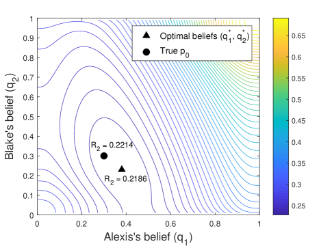
Figure 3: The Bayes risk for q1,q2(0,1)subscript𝑞1subscript𝑞201q_{1},q_{2}\in(0,1) with p0=0.3subscript𝑝00.3p_{0}=0.3, c10=c01=1subscript𝑐10subscript𝑐011c_{10}=c_{01}=1, and additive standard Gaussian noise. The pair of optimal beliefs (\blacktriangle) yields R2=0.2186subscript𝑅20.2186R_{2}=0.2186, while the true prior (\bullet) yields R2=0.2214subscript𝑅20.2214R_{2}=0.2214.

We now focus on Gaussian likelihoods and study their optimal beliefs in this section. Suppose the n𝑛nth agent receives the signal Yn=H+Znsubscript𝑌𝑛𝐻subscript𝑍𝑛Y_{n}=H+Z_{n}, where Znsubscript𝑍𝑛Z_{n} is an independent additive Gaussian noise with zero mean and variance σn2>0superscriptsubscript𝜎𝑛20\sigma_{n}^{2}>0. Thus, the received signal probability densities for H=h𝐻H=h are

fYn|H(yn|h)=ϕ(yn;h,σn2).subscript𝑓conditionalsubscript𝑌𝑛𝐻conditionalsubscript𝑦𝑛italic-ϕsubscript𝑦𝑛superscriptsubscript𝜎𝑛2\displaystyle f_{Y_{n}|H}(y_{n}|h)=\phi(y_{n};h,\sigma_{n}^{2}).

For a belief qnsubscript𝑞𝑛q_{n}, the decision threshold is then determined by the likelihood ratio test,

n(yn)=fYn|H(yn|1)fYn|H(yn|0)H^1=0H^1=1c10qnc01(1qn),subscript𝑛subscript𝑦𝑛subscript𝑓conditionalsubscript𝑌𝑛𝐻conditionalsubscript𝑦𝑛1subscript𝑓conditionalsubscript𝑌𝑛𝐻conditionalsubscript𝑦𝑛0subscript^𝐻10subscript^𝐻11greater-than-or-less-thansubscript𝑐10subscript𝑞𝑛subscript𝑐011subscript𝑞𝑛\displaystyle\mathcal{L}_{n}(y_{n})=\frac{f_{Y_{n}|H}(y_{n}|1)}{f_{Y_{n}|H}(y_{n}|0)}\underset{\widehat{H}_{1}=0}{\overset{\widehat{H}_{1}=1}{\gtrless}}\frac{c_{10}q_{n}}{c_{01}(1-q_{n})},

that simplifies to the following simple threshold condition for Gaussian likelihoods:

ynH^1=0H^1=1λn(qn)=12+σn2log(c10qnc01(1qn)).subscript𝑦𝑛subscript^𝐻10subscript^𝐻11greater-than-or-less-thansubscript𝜆𝑛subscript𝑞𝑛12superscriptsubscript𝜎𝑛2subscript𝑐10subscript𝑞𝑛subscript𝑐011subscript𝑞𝑛\displaystyle y_{n}\underset{\widehat{H}_{1}=0}{\overset{\widehat{H}_{1}=1}{\gtrless}}\lambda_{n}(q_{n})=\frac{1}{2}+\sigma_{n}^{2}\log\left(\frac{c_{10}q_{n}}{c_{01}(1-q_{n})}\right). (28)

Here the index n𝑛n represents the n𝑛nth agent in the system, as the belief and variance of the agent varies along the chain.
Refer to caption
(a) c10=c01=1subscript𝑐10subscript𝑐011c_{10}=c_{01}=1
Refer to caption
(b) c10=1,c01=3formulae-sequencesubscript𝑐101subscript𝑐013c_{10}=1,c_{01}=3
Figure 4: The trend of the optimal beliefs for N=2𝑁2N=2 (Alexis, Blake). Z1,Z2subscript𝑍1subscript𝑍2Z_{1},Z_{2} are standard Gaussian.
Refer to caption
(a) c10=c01=1subscript𝑐10subscript𝑐011c_{10}=c_{01}=1
Refer to caption
(b) c10=1,c01=3formulae-sequencesubscript𝑐101subscript𝑐013c_{10}=1,c_{01}=3
Figure 5: The trend of the optimal beliefs for N=3𝑁3N=3 (Alexis, Blake, and Chuck). Z1,Z2,Z3subscript𝑍1subscript𝑍2subscript𝑍3Z_{1},Z_{2},Z_{3} are standard Gaussian.
Refer to caption
Figure 6: Optimal beliefs when the preceding agent has smaller noise, where σ12=0.8superscriptsubscript𝜎120.8\sigma_{1}^{2}=0.8 and σ22=1superscriptsubscript𝜎221\sigma_{2}^{2}=1.
Refer to caption
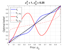
Figure 7: Optimal beliefs when the later-acting agent has smaller noise, where σ12=1superscriptsubscript𝜎121\sigma_{1}^{2}=1 and σ22=0.25superscriptsubscript𝜎220.25\sigma_{2}^{2}=0.25.

Using the recursive update in Sec. III and decision threshold (28), it is possible to obtain the Bayes risk of Blake (i.e., N=2𝑁2N=2) for given beliefs q1,q2subscript𝑞1subscript𝑞2q_{1},q_{2}. Fig. 3 depicts Blake’s Bayes risk for q1,q2(0,1)subscript𝑞1subscript𝑞201q_{1},q_{2}\in(0,1), and explicitly shows that knowing true prior probability is not optimal. The social learning problem with Bayes costs c10=c01=1subscript𝑐10subscript𝑐011c_{10}=c_{01}=1, prior p0=0.3subscript𝑝00.3p_{0}=0.3, and additive Gaussian noise with zero mean and unit variance results in a Bayes risk that is minimum when Alexis’s belief is 0.380.380.38 and Blake’s belief is 0.230.230.23, shown in the figure (triangle) and is compared to the true prior (circle).

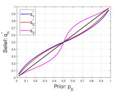
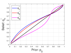
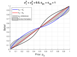
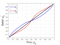
Figs. 4 and 5 show the trend of optimal belief pair that minimizes the last agent’s Bayes risk, when all agents have the same noise levels for the case of two and three agents respectively. We can observe several common characteristics. First, the non-terminal agents (i.e., Alexis for N=2𝑁2N=2 and Alexis and Blake for N=3𝑁3N=3) overweight their beliefs if p0subscript𝑝0p_{0} is small and underweight it if p0subscript𝑝0p_{0} is large. We call this open-minded behavior as it enhances less likely events. Second, the last agent (i.e., Blake for N=2𝑁2N=2 and Chuck for N=3𝑁3N=3) underweights the belief if p0subscript𝑝0p_{0} is small and overweights it if p0subscript𝑝0p_{0} is large, implicitly compensating for the biases of the preceding agents. Such behavior is referred to as being closed-minded as it represents a cautious outlook to the decision-making problem. Lastly, there is a unique, non-trivial prior, p0(0,1)subscript𝑝001p_{0}\in(0,1), where all agents’ optimal beliefs are identical to the true prior.

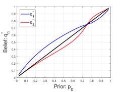
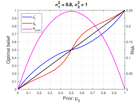
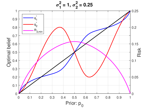
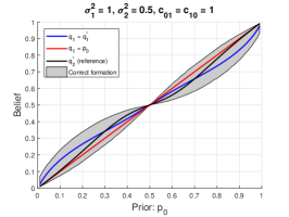
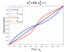
However, the case of nonidentical noise variances of agents results in a very different behavior of optimal beliefs, especially when the last agent has smaller noise. The optimal beliefs for N=2𝑁2N=2 and the case of the preceding agent having smaller noise, and that of the last agent having smaller noise respectively are shown in Figs. 6 and 7. As can be observed, the optimal belief curves are markedly different when the last agent has smaller noise, and we now derive some analytical properties of q1,q2superscriptsubscript𝑞1superscriptsubscript𝑞2q_{1}^{*},q_{2}^{*}.

Theorem 5

For any σ12superscriptsubscript𝜎12\sigma_{1}^{2} and σ22superscriptsubscript𝜎22\sigma_{2}^{2}, q1superscriptsubscript𝑞1q_{1}^{*} and q2superscriptsubscript𝑞2q_{2}^{*} satisfy:

  1. 1.

    for p0(0,1)subscript𝑝001p_{0}\in(0,1), q1p0superscriptsubscript𝑞1subscript𝑝0q_{1}^{*}\leq p_{0} if and only if q2c01c01+c10superscriptsubscript𝑞2subscript𝑐01subscript𝑐01subscript𝑐10q_{2}^{*}\geq\frac{c_{01}}{c_{01}+c_{10}}, with equality for q2=c01c01+c10superscriptsubscript𝑞2subscript𝑐01subscript𝑐01subscript𝑐10q_{2}^{*}=\frac{c_{01}}{c_{01}+c_{10}}.

  2. 2.

    p0=q1=q2subscript𝑝0superscriptsubscript𝑞1superscriptsubscript𝑞2p_{0}=q_{1}^{*}=q_{2}^{*} if and only if p0{0,c01c01+c10,1}subscript𝑝00subscript𝑐01subscript𝑐01subscript𝑐101p_{0}\in\left\{0,\frac{c_{01}}{c_{01}+c_{10}},1\right\}.

Proof:

Given in App. A. ∎

Thm. 5 highlights the fact that if the last agent believes the null hypothesis is more likely, then the ideal predecessor underweights the prior, and vice versa. Additionally, for p0subscript𝑝0p_{0} near zero (near one) the optimal predecessor overweights (underweights) the prior.

In particular, let us consider two cases separately. First, let the predecessor have smaller noise. Then the curves for optimal beliefs and the corresponding Bayes risk are as shown in Fig. 6. The behavior here is similar to the case with equal noise, indicating that the reducing noise of the predecessor does not alter the overall behaviors of beliefs, as the last agent is unaware of this improved signal quality.

On the other hand, when the last agent has smaller noise, we notice that the nature of curves changes, as shown in Fig. 7. The behavior of the ideal agents indicates that when the predecessor has significantly larger noise than the last agent, the last agent stays open-minded. In addition, q1superscriptsubscript𝑞1q_{1}^{*} has multiple crossings with p0subscript𝑝0p_{0}, but q2superscriptsubscript𝑞2q_{2}^{*} has a single crossing at q2=c01/(c01+c10)superscriptsubscript𝑞2subscript𝑐01subscript𝑐01subscript𝑐10q_{2}^{*}=c_{01}/(c_{01}+c_{10}).

As expected, the ideal predecessor is open-minded for near-deterministic priors (p0subscript𝑝0p_{0} close to zero or one). However, when the prior uncertainty in the hypotheses is high (p0subscript𝑝0p_{0} near 1/2121/2), we note that the ideal last agent with less noise favors the less likely hypothesis. This can be attributed to the fact that the last agent stays open-minded to the less likely hypothesis when the predecessor with larger noise is more likely to make errors. To further understand the nature of such an predecessor, we characterize the crossings of the optimal belief curve with the prior q1=p0superscriptsubscript𝑞1subscript𝑝0q_{1}^{*}=p_{0} .

Theorem 6

The set of all p0subscript𝑝0p_{0} such that q1=p0superscriptsubscript𝑞1subscript𝑝0q_{1}^{*}=p_{0}, q2=c01c01+c10superscriptsubscript𝑞2subscript𝑐01subscript𝑐01subscript𝑐10q_{2}^{*}=\frac{c_{01}}{c_{01}+c_{10}} is given by the solutions to

ex=1βQ(α+σ1x)1βQ(ασ1x),superscript𝑒𝑥1𝛽𝑄𝛼subscript𝜎1𝑥1𝛽𝑄𝛼subscript𝜎1𝑥\displaystyle e^{x}=\frac{1-\beta Q(-\alpha+\sigma_{1}x)}{1-\beta Q(-\alpha-\sigma_{1}x)}, (29)

where

x=log(c10p0c01(1p0)),α=12σ1,β=1Q(1/2σ2)Q(1/2σ2).formulae-sequence𝑥subscript𝑐10subscript𝑝0subscript𝑐011subscript𝑝0formulae-sequence𝛼12subscript𝜎1𝛽1𝑄12subscript𝜎2𝑄12subscript𝜎2\displaystyle x=\log\left(\frac{c_{10}p_{0}}{c_{01}(1-p_{0})}\right),~{}\alpha=\frac{1}{2\sigma_{1}},~{}\beta=1-\frac{Q\left(1/2\sigma_{2}\right)}{Q\left(-1/2\sigma_{2}\right)}.
Proof:

Given in App. B. ∎

We note that p=c01c01+c10superscript𝑝subscript𝑐01subscript𝑐01subscript𝑐10p^{*}=\frac{c_{01}}{c_{01}+c_{10}} is always a solution to (29). The case of multiple solutions to (29) is of particular interest and a sufficient condition is given in the following corollary.

Corollary 2

If

2βσ1ϕ(α)1βQ(α)>1,2𝛽subscript𝜎1italic-ϕ𝛼1𝛽𝑄𝛼1\frac{2\beta\sigma_{1}\phi{(\alpha)}}{1-\beta Q(-\alpha)}>1, (30)

then, (29) has at least 333 solutions in (0,1)01(0,1).

Proof:

Since x𝑥x is a monotonic function of p0subscript𝑝0p_{0}, it is sufficient to show that (29) has at least 333 solutions in x𝑥x. From the symmetry in (29), since x=0𝑥0x=0 is always a root, it suffices to show the existence of at least one more root in x>0𝑥0x>0. First note the ranges of variables, x(,),α(0,),β(0,1)formulae-sequence𝑥formulae-sequence𝛼0𝛽01x\in(-\infty,\infty),\alpha\in(0,\infty),\beta\in(0,1).

Letting r(x)𝑟𝑥r(x) be the right side of (29), since 0Q()10𝑄10\leq Q(\cdot)\leq 1, we have

1βr(x):=1βQ(α+σ1x)1βQ(ασ1x)11β,1𝛽𝑟𝑥assign1𝛽𝑄𝛼subscript𝜎1𝑥1𝛽𝑄𝛼subscript𝜎1𝑥11𝛽\displaystyle 1-\beta\leq r(x):=\frac{1-\beta Q(-\alpha+\sigma_{1}x)}{1-\beta Q(-\alpha-\sigma_{1}x)}\leq\frac{1}{1-\beta},

indicating that r(x)[1β,11β]𝑟𝑥1𝛽11𝛽r(x)\in[1-\beta,\tfrac{1}{1-\beta}]. However, note that exsuperscript𝑒𝑥e^{x} monotonically increases in (1,)1(1,\infty) for x>0𝑥0x>0. Since ex,r(x)superscript𝑒𝑥𝑟𝑥e^{x},r(x) coincide at x=0𝑥0x=0, it follows that they cross at least once on (0,)0(0,\infty) and also on (,0)0(-\infty,0), if r(x)>ddxexsuperscript𝑟𝑥𝑑𝑑𝑥superscript𝑒𝑥r^{\prime}(x)>\tfrac{d}{dx}e^{x} at x=0𝑥0x=0 by the intermediate value theorem. Thus, the sufficient condition follows:

r(0)=2σ1βϕ(α;0,1)1βQ(α)>1=ddxex|x=0.superscript𝑟02subscript𝜎1𝛽italic-ϕ𝛼011𝛽𝑄𝛼1evaluated-at𝑑𝑑𝑥superscript𝑒𝑥𝑥0\displaystyle r^{\prime}(0)=\frac{2\sigma_{1}\beta\phi(\alpha;0,1)}{1-\beta Q(-\alpha)}>1=\frac{d}{dx}e^{x}\Bigg{|}_{x=0}.

Refer to caption
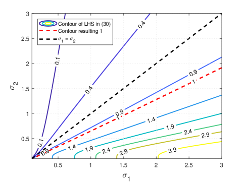
Figure 8: Contour plot of (30) with values for various σ1,σ2subscript𝜎1subscript𝜎2\sigma_{1},\sigma_{2}. The red dotted contour shows the contour that results in 111 so that the area below it satisfies (30) and therefore has multiple solutions to (29).

Cor. 2 provides a sufficient condition on the noise level of agents under which there exists multiple crossings of the curves q1(p0)superscriptsubscript𝑞1subscript𝑝0q_{1}^{*}(p_{0}) and p0subscript𝑝0p_{0}. The range of standard deviations of the additive Gaussian noise of the preceding and last agents that satisfy the sufficient condition of Cor. 2 is shown in Fig. 8. Note from the figure that the area below the red dotted contour in Fig. 8 has multiple solutions to q1=p0superscriptsubscript𝑞1subscript𝑝0q_{1}^{*}=p_{0}, i.e., when the last agent has comparatively smaller than the preceding agent.

This is important as the crossings indicate a change in the perceived bias of the predecessor and also indicates the regions in which the last agent overweights the unlikely hypothesis as in Fig. 7.

VI Team Construction Criterion

Having studied the mathematical conditions for optimal reweighting of initial beliefs, we now investigate team selection for social learning. Naturally, a social planner who is aware of the context p0subscript𝑝0p_{0} can pick the optimal agent pairs to minimize Bayes risk. However, it is not clear if agents are capable of organizing themselves into ideal teams in the absence of contextual knowledge. Thus, we now identify the criterion for the last agent to identify the optimal predecessors among a set of given predecessors.

Theorem 7

Consider two predecessors with q1<q1subscript𝑞1subscript𝑞superscript1q_{1}<q_{1^{\prime}}. Let λ1,λ1subscript𝜆1subscript𝜆superscript1\lambda_{1},\lambda_{1^{\prime}} be the decision thresholds of the respective predecessors. Then, the predecessor with belief q1subscript𝑞1q_{1} is the optimal choice if and only if

1[Y1[λ1,λ1],Y2[λ21,λ20]]0[Y1[λ1,λ1],Y2[λ21,λ20]]c10p0c01(1p0).subscript1delimited-[]formulae-sequencesubscript𝑌1subscript𝜆1subscript𝜆superscript1subscript𝑌2superscriptsubscript𝜆21superscriptsubscript𝜆20subscript0delimited-[]formulae-sequencesubscript𝑌1subscript𝜆1subscript𝜆superscript1subscript𝑌2superscriptsubscript𝜆21superscriptsubscript𝜆20subscript𝑐10subscript𝑝0subscript𝑐011subscript𝑝0\frac{\mathbb{P}_{1}\left[Y_{1}\in[\lambda_{1},\lambda_{1^{\prime}}],Y_{2}\in[\lambda_{2}^{1},\lambda_{2}^{0}]\right]}{\mathbb{P}_{0}\left[Y_{1}\in[\lambda_{1},\lambda_{1^{\prime}}],Y_{2}\in[\lambda_{2}^{1},\lambda_{2}^{0}]\right]}\geq\frac{c_{10}p_{0}}{c_{01}(1-p_{0})}. (31)
Proof:

Given in App. C. ∎

In other words, by rewriting (31) in a likelihood ratio form, we observe that the criterion for picking the predecessor with a smaller belief is given by the likelihood ratio test

[H^1=H^2=1,H^1=H^2=0]c10p0c01(1p0),{\mathcal{L}}\left[\widehat{H}_{1}=\widehat{H}_{2}=1,\widehat{H}_{1^{\prime}}=\widehat{H}_{2^{\prime}}=0\right]\geq\frac{c_{10}p_{0}}{c_{01}(1-p_{0})},

where H^2subscript^𝐻superscript2\widehat{H}_{2^{\prime}} is the decision made by the last agent following the decision of the predecessor with belief q1subscript𝑞superscript1q_{1^{\prime}}.

Thus selecting an ideal predecessor requires a social planner who is aware of the context p0subscript𝑝0p_{0}. Without this, the last agent selects an predecessor according to his personal belief q2subscript𝑞2q_{2}. That is, the last agent verifies condition (31) by replacing p0subscript𝑝0p_{0} by q2subscript𝑞2q_{2}. Such a choice of predecessor might not always conform to the optimal choice when the belief of the last agent deviates significantly from the prior. To illustrate, we consider the problem of choosing between two predecessors with beliefs q1(p0)=q1(p0)subscript𝑞1subscript𝑝0superscriptsubscript𝑞1subscript𝑝0q_{1}(p_{0})=q_{1}^{*}(p_{0}) and q1(p0)=p0subscript𝑞superscript1subscript𝑝0subscript𝑝0q_{1^{\prime}}(p_{0})=p_{0}. Let q(p0,q2)𝑞subscript𝑝0subscript𝑞2q(p_{0},q_{2}) be the belief of the optimal predecessor choice for a given pair (p0,q2)subscript𝑝0subscript𝑞2(p_{0},q_{2}). We identify the region of correct selection by shading, 𝒮={(p0,q2):q(p0,q2)=q(q2,q2)}𝒮conditional-setsubscript𝑝0subscript𝑞2𝑞subscript𝑝0subscript𝑞2𝑞subscript𝑞2subscript𝑞2{\mathcal{S}}=\{(p_{0},q_{2}):q(p_{0},q_{2})=q(q_{2},q_{2})\}.

Refer to caption
(a) Predecessor selection under equal noise. The optimal later-acting agent fails to recognize the optimal predecessor and makes mistakes often. The trend is similar in cases with smaller noise predecessor.
Refer to caption
(b) Predecessor selection under noise diversity. The optimal later-acting agent selects the optimal predecessor in this case.
Refer to caption
(c) Context-unaware predecessor selection. The last agent chooses predecessor using (32) without p0subscript𝑝0p_{0} and the Bayes risk increases as a result.
Figure 9: Context-unaware team selection.

First, when noise levels are equal, the region in which the last agent picks the correct preceding agent is shown in Fig. 9(a). We note that the correct region is relatively small and does not include q2superscriptsubscript𝑞2q_{2}^{*}. In particular, the last agent with optimal belief chooses the wrong predecessor always, whereas a suboptimal last agent with beliefs in the shaded region picks the correct one.

On the other hand, when the last agent has smaller noise than the predecessor, the corresponding region is as shown in Fig. 9(b). Here we note that the last agent with optimal belief picks the correct preceding agent always.

Thus, we note that knowledge of the mathematically optimal beliefs does not guarantee selection of the right preceding agent. Further, we also observe that the diversity of noise levels may increase the feasibility of selecting the right preceding agent when the last agent has optimal belief.

We also explore the optimal choice of predecessor for the given optimal last agent in the absence of knowledge of the prior probability. From (25), the belief of the optimal preceding agent, q~1subscript~𝑞1\tilde{q}_{1} chosen by an last agent, in the absence of context (prior probability p0subscript𝑝0p_{0}) satisfies

q~11q~1=p01p0Pe,2I1Pe,2I0Pe,2II0Pe,2II1.subscript~𝑞11subscript~𝑞1subscript𝑝01subscript𝑝0superscriptsubscript𝑃𝑒2subscriptI1superscriptsubscript𝑃𝑒2subscriptI0superscriptsubscript𝑃𝑒2subscriptII0superscriptsubscript𝑃𝑒2subscriptII1\frac{\tilde{q}_{1}}{1-\tilde{q}_{1}}=\frac{p_{0}}{1-p_{0}}\frac{P_{e,2}^{\textup{I}_{1}}-P_{e,2}^{\textup{I}_{0}}}{P_{e,2}^{\textup{II}_{0}}-P_{e,2}^{\textup{II}_{1}}}. (32)

The last agent’s behavior with belief q2superscriptsubscript𝑞2q_{2}^{*} is as shown in Fig. 9(c). We note that the preceding agent chosen by the last agent differs from the optimal choice. Further, it is also evident that this choice consequently results in an increased Bayes risk. Such behavior in team selection highlights the significance of context and thus a social planner for identifying the right team.

VII Human-AI Collaboration Systems

In this section, we use mathematical results from previous sections to study the engineering design problem of constructing human-AI collaborative systems. To do so, we make the following assumptions from the behavioral sciences: Human agents perform Bayesian decision-making [42, 43, 44, 45] and their perceptions follow the Prelec reweighting function [38]. In addition, agents experience varying observational noise which is additive and Gaussian (as it is a common model in human signal perception [46, 47]). As usual in sequential social learning setup, all agents make selfish decisions [6, 10].

VII-A Approximation by Prelec Family

To design human-AI collaborative systems, we first determine whether optimal belief functions from previous sections are close to human behavior as modeled by cumulative prospect theory [35, 38].555Bounded rationality models have been categorized into two main classes—costly bounded rationality and truly bounded rationality [48]. Costly rationality considers the emergence of boundedly irrational behavior as optimization under some costs of decision-making such as computation and communication. On the other hand, truly bounded rationality is not based on an optimization framework. Though not the focus of the present paper, one might wonder whether people are (approximately) naturally optimal for social learning. That is, do cumulative prospect-theoretic models emerge from a costly rationality framework for social learning, since the optimal belief curves result from limitations in computation (selfish decision-making) and communication (public signal quantization).

We approximate the optimal belief curves qnsuperscriptsubscript𝑞𝑛q_{n}^{*} by the Prelec function and study the resulting increase in the Bayes risk. We restrict to the Prelec family whose fixed point is identical to p=c10c01+c10superscript𝑝subscript𝑐10subscript𝑐01subscript𝑐10p^{*}=\frac{c_{10}}{c_{01}+c_{10}}, and then find best parameters (αn,βn)subscript𝛼𝑛subscript𝛽𝑛(\alpha_{n},\beta_{n}) in the minimax absolute error sense, i.e.,

(αn,βn)=argminα,β:w(p;α,β)=pqn()w(;α,β).subscript𝛼𝑛subscript𝛽𝑛subscriptargmin:𝛼𝛽𝑤superscript𝑝𝛼𝛽superscript𝑝subscriptnormsuperscriptsubscript𝑞𝑛𝑤𝛼𝛽\displaystyle(\alpha_{n},\beta_{n})=\operatorname*{arg\,min}_{\alpha,\beta:w\left(p^{*};\alpha,\beta\right)=p^{*}}\|q_{n}^{*}(\cdot)-w(\cdot;\alpha,\beta)\|_{\infty}.

Let the Prelec function approximations be (q1,Pre,q2,Pre)subscript𝑞1Presubscript𝑞2Pre(q_{1,\textrm{Pre}},q_{2,\textrm{Pre}}).

Refer to caption
(a) When the preceding agent has smaller noise.
Refer to caption
(b) When the later-acting agent has smaller noise
Figure 10: Optimal beliefs as compared to Prelec-weighted beliefs.

The Prelec approximations for the two-agent case are shown in dotted curves in Fig. 10. When the preceding agent has smaller noise as in Fig. 10(a), the Prelec function approximates the optimal beliefs well and the Bayes risk does not increase by much. To evaluate the loss from the approximation, consider the set of correct beliefs q1=q2=p0subscript𝑞1subscript𝑞2subscript𝑝0q_{1}=q_{2}=p_{0}, that result in a Bayes risk of R2,corrsubscript𝑅2corrR_{2,\textrm{corr}}. The maximal loss in terms of Bayes risk from using the correct beliefs is maxp0(R2,corrR2,min)0.0039subscriptsubscript𝑝0subscript𝑅2corrsubscript𝑅2min0.0039\max_{p_{0}}(R_{2,\textrm{corr}}-R_{2,\textrm{min}})\approx 0.0039. On the other hand, the maximal loss from the best Prelec approximation is 0.0009absent0.0009\approx 0.0009. This indicates that the natural cognitive biases of humans (i.e., Prelec reweighting) are effective for social learning when the preceding agent has smaller noise.

On the other hand, when the last agent has smaller noise as in Fig. 10(b), the Prelec approximation does not accurately mimic the optimal behavior of agents. Recall that the Prelec function is always increasing and has only one crossing with unit slope line in (0,1)01(0,1). Therefore, the Prelec function fails to account for all the variations in the optimal belief. Moreover, while the additional loss of Bayes risk by the Prelec fitting is 0.0187absent0.0187\approx 0.0187, the loss from using the correct beliefs, p0=q1=q2subscript𝑝0subscript𝑞1subscript𝑞2p_{0}=q_{1}=q_{2}, is 0.0060absent0.0060\approx 0.0060. This indicates that even though the Prelec weighting functions serve as good approximations with predecessors having less noisy observations, they do not model the optimal behavior in the case of predecessors having noisier observations. These results suggest that human agents following cumulative prospect theory models [35] yield small Bayes risk when predecessors have smaller noise.

Refer to caption
(a)
Refer to caption
(b)
Figure 11: Models of AI-human collaboration, where a machine provides input for human judgement or vice versa.

VII-B Human-AI Teams

The previous subsection informs the design of AI-human collaboration structures [34]. In many human-AI joint teams, a human agent makes the final decision based on the advice of an AI component as depicted in Fig. 11(a), but the opposite structure of Fig. 11(b) is also possible. It is thus important to identify the best team configuration [48]. Indeed, D. Kahneman recently stated that “You can combine humans and machines, provided the machine has the last word” [49].

Our results indicate that an AI assistant with smaller noise could be an effective predecessor to the human decision-maker. In particular, an open-minded AI predecessor and a closed-minded human final decision-maker with appropriate Prelec reweighted beliefs work well together, as in Fig. 6. However, an AI component with greater noise might not be a good predecessor to the human last agent who does not have beliefs that mimic the optimal behavior in Fig. 7 and so perhaps counterintuitively, the architecture of Fig. 11(b) should be adopted, with the AI agent having larger noise making the global decision.

Additionally, these results along with those of Sec. VI provide some insight into human-AI teams when the human agent picks an AI predecessor, given a choice among different agents. In particular, consider the AI-human team where the human, who has a Prelec-weighted belief, chooses one of two possible AI predecessors—one that has the optimal belief q1superscriptsubscript𝑞1q_{1}^{*} and the other that is aware of the true prior p0subscript𝑝0p_{0}. In case the human agent has larger noise, and a closed-minded Prelec belief as in Fig. 9(a), she unfortunately picks the AI predecessor with q1=p0subscript𝑞1subscript𝑝0q_{1}=p_{0} and the team becomes suboptimal. However, if the human agent has smaller noise, and an open-minded Prelec belief, she picks the optimal AI component q1=q1subscript𝑞1superscriptsubscript𝑞1q_{1}=q_{1}^{*} and therefore can make the optimal decision as in Fig. 9(b). Thus it is evident that optimal team organization is feasible when the human has smaller noise and the appropriate open-minded belief.

VIII Conclusion

We discussed the sequential social learning problem with individual biased beliefs. Unlike previous works on herding, we focused on the Bayes risk of the last-acting agent. We first derived the optimal belief update rule for general likelihoods and evaluated for Gaussian likelihoods. Counterintuitively, optimal beliefs that yield minimum Bayes risk are in general different from the true prior. Under equal noise levels, we observed that optimal preceding agents have open-minded beliefs, that is, overweight small priors and underweight large priors, while the optimal last agent has closed-minded belief. However, the trend may change depending on varying noise levels such that especially when the last agent has much smaller noise, optimal belief of the last agent is inverted as she becomes open-minded.

We also showed that the Prelec reweighting function from cumulative prospect theory approximates the behavior of the optimal beliefs under specific levels of noise, however, when the last agent has much smaller noise, it fails to capture all the behavioral traits of the optimal beliefs.

Finally, we considered the ability of agents to organize themselves into optimal teams and showed that in the absence of a social planner, the last agent can get paired with the wrong predecessor when the individual belief deviates significantly from the underlying prior value. The setup arises from the consideration of AI and it tells us without knowing the true prior, our human-machine team construction could be misorganized.

Appendix A Proof of Theorem 5

Let us prove Thm. 5 starting with the premise that q1p0superscriptsubscript𝑞1subscript𝑝0q_{1}^{*}\geq p_{0}. First, from (25), we have

q1p0superscriptsubscript𝑞1subscript𝑝0\displaystyle q_{1}^{*}\geq p_{0} Pe,2II1Pe,2II0Pe,2I1Pe,2I01.iffabsentsuperscriptsubscript𝑃𝑒2subscriptII1superscriptsubscript𝑃𝑒2subscriptII0superscriptsubscript𝑃𝑒2subscriptI1superscriptsubscript𝑃𝑒2subscriptI01\displaystyle\iff\frac{P_{e,2}^{\textup{II}_{1}}-P_{e,2}^{\textup{II}_{0}}}{P_{e,2}^{\textup{I}_{1}}-P_{e,2}^{\textup{I}_{0}}}\geq-1. (33)

To study the ratio in (33), consider the Type I vs. Type II error curve for binary hypothesis testing under additive Gaussian noise.666It is also called Receiver Operating Characteristic (ROC) curve [50, 51] when the curve is vertically inverted. This is shown in Fig. 12, and as seen here is a convex function [50]. Note that on the curve, the Type I and Type II error probabilities, (PeI,PeII)superscriptsubscript𝑃𝑒Isuperscriptsubscript𝑃𝑒II(P_{e}^{\textup{I}},P_{e}^{\textup{II}}), are the points on the curve that have tangents with slope matching (c10qc01(1q))subscript𝑐10𝑞subscript𝑐011𝑞-\left(\tfrac{c_{10}q}{c_{01}(1-q)}\right), where q𝑞q is the corresponding probability, and σ2superscript𝜎2\sigma^{2} is the variance of the additive Gaussian noise.

First, from Thm. 2, we know that q20q21superscriptsubscript𝑞20superscriptsubscript𝑞21q_{2}^{0}\geq q_{2}^{1} which in turn implies that λ20λ21superscriptsubscript𝜆20superscriptsubscript𝜆21\lambda_{2}^{0}\geq\lambda_{2}^{1}. This in turn indicates that

Pe,2I0=Q(λ20σ2)Q(λ21σ2)=Pe,2I1.superscriptsubscript𝑃𝑒2subscriptI0𝑄superscriptsubscript𝜆20subscript𝜎2𝑄superscriptsubscript𝜆21subscript𝜎2superscriptsubscript𝑃𝑒2subscriptI1P_{e,2}^{\textup{I}_{0}}=Q\left(\tfrac{\lambda_{2}^{0}}{\sigma_{2}}\right)\leq Q\left(\tfrac{\lambda_{2}^{1}}{\sigma_{2}}\right)=P_{e,2}^{\textup{I}_{1}}.

Similarly, Pe,2II0Pe,2II1superscriptsubscript𝑃𝑒2subscriptII0superscriptsubscript𝑃𝑒2subscriptII1P_{e,2}^{\textup{II}_{0}}\geq P_{e,2}^{\textup{II}_{1}}, and thus, as shown in the figure, the point B0=(Pe,2I0,Pe,2II0)subscript𝐵0superscriptsubscript𝑃𝑒2subscriptI0superscriptsubscript𝑃𝑒2subscriptII0B_{0}=\left(P_{e,2}^{\textup{I}_{0}},P_{e,2}^{\textup{II}_{0}}\right) lies to the left of B1=(Pe,2I1,Pe,2II1)subscript𝐵1superscriptsubscript𝑃𝑒2subscriptI1superscriptsubscript𝑃𝑒2subscriptII1B_{1}=\left(P_{e,2}^{\textup{I}_{1}},P_{e,2}^{\textup{II}_{1}}\right).

Further, since B1subscript𝐵1B_{1} lies on the curve, so does the point B¯1=(Pe,2II1,Pe,2I1)subscript¯𝐵1superscriptsubscript𝑃𝑒2subscriptII1superscriptsubscript𝑃𝑒2subscriptI1\bar{B}_{1}=\left(P_{e,2}^{\textup{II}_{1}},P_{e,2}^{\textup{I}_{1}}\right) as it caters to the error probabilities corresponding to the probability of the null hypothesis H=0=1q21𝐻01superscriptsubscript𝑞21\mathbb{P}{H=0}=1-q_{2}^{1}. Thus, the line B1B¯1¯¯subscript𝐵1subscript¯𝐵1\overline{B_{1}\bar{B}_{1}} has a slope of 11-1.

Note that the condition (33) translates to the slope of the line B0B1¯¯subscript𝐵0subscript𝐵1\overline{B_{0}B_{1}} is greater than 11-1. Observe that if B¯1subscript¯𝐵1\bar{B}_{1} lies to the right of B1subscript𝐵1B_{1} then it implies that the slope of B0B1¯¯subscript𝐵0subscript𝐵1\overline{B_{0}B_{1}} is less than 11-1, violating (33). Similarly, if B0subscript𝐵0B_{0} lies to the left of B¯1subscript¯𝐵1\bar{B}_{1}, then again the (33) is violated.

On the other hand, if B0subscript𝐵0B_{0} lies between B¯1subscript¯𝐵1\bar{B}_{1} and B1subscript𝐵1B_{1}, then we know that the slope of B0B1¯¯subscript𝐵0subscript𝐵1\overline{B_{0}B_{1}} is greater than that of B1B¯1¯¯subscript𝐵1subscript¯𝐵1\overline{B_{1}\bar{B}_{1}}, therein satisfying (33). Thus, (33) is true if and only if the point B0subscript𝐵0B_{0} lies between the two points B1subscript𝐵1B_{1} and B¯1subscript¯𝐵1\bar{B}_{1}.

Refer to caption
Figure 12: The point B0subscript𝐵0B_{0} always exists between points B1subscript𝐵1B_{1} and B¯1subscript¯𝐵1\bar{B}_{1}.

From the convexity of the curve and comparing coordinates of B0subscript𝐵0B_{0} and B¯1subscript¯𝐵1\bar{B}_{1}, we have

q1p0superscriptsubscript𝑞1subscript𝑝0\displaystyle q_{1}^{*}\geq p_{0}
Pe,2I0Pe,2II1 and Pe,2II0Pe,2I1iffabsentsuperscriptsubscript𝑃𝑒2subscriptI0superscriptsubscript𝑃𝑒2subscriptII1 and superscriptsubscript𝑃𝑒2subscriptII0superscriptsubscript𝑃𝑒2subscriptI1\displaystyle\iff P_{e,2}^{\textup{I}_{0}}\geq P_{e,2}^{\textup{II}_{1}}\text{ and }P_{e,2}^{\textup{II}_{0}}\leq P_{e,2}^{\textup{I}_{1}}
(a)Q(λ20σ2)1Q(λ211σ2)superscriptiff𝑎absent𝑄superscriptsubscript𝜆20subscript𝜎21𝑄superscriptsubscript𝜆211subscript𝜎2\displaystyle\stackrel{{\scriptstyle(a)}}{{\iff}}Q\left(\frac{\lambda_{2}^{0}}{\sigma_{2}}\right)\geq 1-Q\left(\frac{\lambda_{2}^{1}-1}{\sigma_{2}}\right)
 and Q(λ21σ2)1Q(λ201σ2) and 𝑄superscriptsubscript𝜆21subscript𝜎21𝑄superscriptsubscript𝜆201subscript𝜎2\displaystyle~{}~{}~{}\text{ and }Q\left(\frac{\lambda_{2}^{1}}{\sigma_{2}}\right)\geq 1-Q\left(\frac{\lambda_{2}^{0}-1}{\sigma_{2}}\right)
(b)λ20+λ211superscriptiff𝑏absentsuperscriptsubscript𝜆20superscriptsubscript𝜆211\displaystyle\stackrel{{\scriptstyle(b)}}{{\iff}}\lambda_{2}^{0}+\lambda_{2}^{1}\leq 1
(c)2λ1,[2]+σ22log(Pe,1,[2]I(1Pe,1,[2]I)Pe,1,[2]II(1Pe,1,[2]II))1,superscriptiff𝑐absent2subscript𝜆1delimited-[]2superscriptsubscript𝜎22superscriptsubscript𝑃𝑒1delimited-[]2I1superscriptsubscript𝑃𝑒1delimited-[]2Isuperscriptsubscript𝑃𝑒1delimited-[]2II1superscriptsubscript𝑃𝑒1delimited-[]2II1\displaystyle\stackrel{{\scriptstyle(c)}}{{\iff}}2\lambda_{1,[2]}+\sigma_{2}^{2}\log\left(\frac{P_{e,1,[2]}^{\textup{I}}\left(1-P_{e,1,[2]}^{\textup{I}}\right)}{P_{e,1,[2]}^{\textup{II}}\left(1-P_{e,1,[2]}^{\textup{II}}\right)}\right)\leq 1, (34)

where (a) follows from the false alarm and missed detection probabilities in terms of the Q𝑄Q-function of the standard Gaussian random variable; (b) follows from the fact that the Q𝑄Q-function is monotonically decreasing and that 1Q(x)=Q(x)1𝑄𝑥𝑄𝑥1-Q(x)=Q(-x); and (c) follows from (22), (23), and λ1,[2]=λ2(q2)subscript𝜆1delimited-[]2subscript𝜆2subscript𝑞2\lambda_{1,[2]}=\lambda_{2}(q_{2}).

From (28), we have

λ1,[2]=12+σ22log(c10q2c01(1q2)).subscript𝜆1delimited-[]212superscriptsubscript𝜎22subscript𝑐10superscriptsubscript𝑞2subscript𝑐011superscriptsubscript𝑞2\lambda_{1,[2]}=\frac{1}{2}+\sigma_{2}^{2}\log\left(\frac{c_{10}q_{2}^{*}}{c_{01}(1-q_{2}^{*})}\right).

Substituting in (34), we have

q1p0superscriptsubscript𝑞1subscript𝑝0\displaystyle q_{1}^{*}\geq p_{0} 2log(c10q2c01(1q2))iffabsent2subscript𝑐10superscriptsubscript𝑞2subscript𝑐011superscriptsubscript𝑞2\displaystyle\iff 2\log\left(\frac{c_{10}q_{2}^{*}}{c_{01}(1-q_{2}^{*})}\right)
log(Pe,1,[2]II(1Pe,1,[2]II)Pe,1,[2]I(1Pe,1,[2]I)).absentsuperscriptsubscript𝑃𝑒1delimited-[]2II1superscriptsubscript𝑃𝑒1delimited-[]2IIsuperscriptsubscript𝑃𝑒1delimited-[]2I1superscriptsubscript𝑃𝑒1delimited-[]2I\displaystyle~{}~{}~{}~{}~{}~{}\leq\log\left(\frac{P_{e,1,[2]}^{\textup{II}}\left(1-P_{e,1,[2]}^{\textup{II}}\right)}{P_{e,1,[2]}^{\textup{I}}\left(1-P_{e,1,[2]}^{\textup{I}}\right)}\right).

Letting x:=log(c10q2c01(1q2))=1σ22(λ212)assign𝑥subscript𝑐10superscriptsubscript𝑞2subscript𝑐011superscriptsubscript𝑞21superscriptsubscript𝜎22subscript𝜆212x:=\log\left(\tfrac{c_{10}q_{2}^{*}}{c_{01}(1-q_{2}^{*})}\right)=\tfrac{1}{\sigma_{2}^{2}}\left(\lambda_{2}-\tfrac{1}{2}\right) and using Q()𝑄Q(\cdot) representation of error probabilities, we have

q1p0superscriptsubscript𝑞1subscript𝑝0\displaystyle q_{1}^{*}\geq p_{0} 2xlog(Q(σ2x12σ2)Q(σ2x+12σ2)Q(σ2x+12σ2)Q(σ2x12σ2)).iffabsent2𝑥𝑄subscript𝜎2𝑥12subscript𝜎2𝑄subscript𝜎2𝑥12subscript𝜎2𝑄subscript𝜎2𝑥12subscript𝜎2𝑄subscript𝜎2𝑥12subscript𝜎2\displaystyle\iff 2x\leq\log\left(\frac{Q\left(\sigma_{2}x-\tfrac{1}{2\sigma_{2}}\right)Q\left(-\sigma_{2}x+\tfrac{1}{2\sigma_{2}}\right)}{Q\left(\sigma_{2}x+\tfrac{1}{2\sigma_{2}}\right)Q\left(-\sigma_{2}x-\tfrac{1}{2\sigma_{2}}\right)}\right). (35)

From Cor. 1, we know that the function

g~(x)=x+log(Q(σx+12σ)Q(σx12σ))~𝑔𝑥𝑥𝑄𝜎𝑥12𝜎𝑄𝜎𝑥12𝜎\tilde{g}(x)=x+\log\left(\frac{Q\left(\sigma x+\tfrac{1}{2\sigma}\right)}{Q\left(\sigma x-\tfrac{1}{2\sigma}\right)}\right)

is an increasing function of x𝑥x. Thus, reformulating (35) using g~()~𝑔\tilde{g}(\cdot),

q1p0superscriptsubscript𝑞1subscript𝑝0\displaystyle q_{1}^{*}\geq p_{0} g~(x)g~(x)iffabsent~𝑔𝑥~𝑔𝑥\displaystyle\iff\tilde{g}(x)\leq\tilde{g}(-x)
x0q2c01c01+c10.\displaystyle\iff x\leq 0\iff q_{2}^{*}\leq\frac{c_{01}}{c_{01}+c_{10}}.

The condition for equality follows from observing the condition for equality at all the inequalities, proving the first part of the result.

The second part follows directly from the first, taking into account the trivial cases of p0{0,1}subscript𝑝001p_{0}\in\{0,1\}.

Appendix B Proof of Theorem 6

We will consider the case of c01=c10=1subscript𝑐01subscript𝑐101c_{01}=c_{10}=1 for convenience. The proof extends directly by a simple scaling argument.

The optimal belief of worker two satisfies R2q2=0subscript𝑅2subscript𝑞20\frac{\partial R_{2}}{\partial q_{2}}=0. Thus, differentiating (24) with respect to q2subscript𝑞2q_{2} and rearranging,

p0[(1Pe,1I)fY2|H(λ20|0)λ20q2+Pe,1IfY2|H(λ21|0)λ21q2]=subscript𝑝0delimited-[]1superscriptsubscript𝑃𝑒1Isubscript𝑓conditionalsubscript𝑌2𝐻conditionalsuperscriptsubscript𝜆200superscriptsubscript𝜆20subscript𝑞2superscriptsubscript𝑃𝑒1Isubscript𝑓conditionalsubscript𝑌2𝐻conditionalsuperscriptsubscript𝜆210superscriptsubscript𝜆21subscript𝑞2absent\displaystyle p_{0}\left[(1-P_{e,1}^{\textup{I}})f_{Y_{2}|H}(\lambda_{2}^{0}|0)\frac{\partial\lambda_{2}^{0}}{\partial q_{2}}+P_{e,1}^{\textup{I}}f_{Y_{2}|H}(\lambda_{2}^{1}|0)\frac{\partial\lambda_{2}^{1}}{\partial q_{2}}\right]=
(1p0)[Pe,1IIfY2|H(λ20|1)λ20q2+(1Pe,1II)fY2|H(λ21|1)λ21q2].1subscript𝑝0delimited-[]superscriptsubscript𝑃𝑒1IIsubscript𝑓conditionalsubscript𝑌2𝐻conditionalsuperscriptsubscript𝜆201superscriptsubscript𝜆20subscript𝑞21superscriptsubscript𝑃𝑒1IIsubscript𝑓conditionalsubscript𝑌2𝐻conditionalsuperscriptsubscript𝜆211superscriptsubscript𝜆21subscript𝑞2\displaystyle(1-p_{0})\left[P_{e,1}^{\textup{II}}f_{Y_{2}|H}(\lambda_{2}^{0}|1)\frac{\partial\lambda_{2}^{0}}{\partial q_{2}}+(1-P_{e,1}^{\textup{II}})f_{Y_{2}|H}(\lambda_{2}^{1}|1)\frac{\partial\lambda_{2}^{1}}{\partial q_{2}}\right].

Let x=log(p01p0)𝑥subscript𝑝01subscript𝑝0x=\log\left(\frac{p_{0}}{1-p_{0}}\right). For q2=1/2superscriptsubscript𝑞212q_{2}^{*}=1/2 and q1=p0superscriptsubscript𝑞1subscript𝑝0q_{1}^{*}=p_{0}, we have

λ1=12+σ12x and λ1,[2]=12.subscript𝜆112superscriptsubscript𝜎12𝑥 and subscript𝜆1delimited-[]212\displaystyle\lambda_{1}=\frac{1}{2}+\sigma_{1}^{2}x\textrm{ and }\lambda_{1,[2]}=\frac{1}{2}.

It implies Pe,1,[2]I=Pe,1,[2]II=Q(1/2σ2)superscriptsubscript𝑃𝑒1delimited-[]2Isuperscriptsubscript𝑃𝑒1delimited-[]2II𝑄12subscript𝜎2P_{e,1,[2]}^{\textup{I}}=P_{e,1,[2]}^{\textup{II}}=Q(1/2\sigma_{2}). Then,

(λ20)superscriptsubscript𝜆20\displaystyle{\mathcal{L}}(\lambda_{2}^{0}) =fY2|H(λ20|1)fY2|H(λ20|0)absentsubscript𝑓conditionalsubscript𝑌2𝐻conditionalsuperscriptsubscript𝜆201subscript𝑓conditionalsubscript𝑌2𝐻conditionalsuperscriptsubscript𝜆200\displaystyle=\frac{f_{Y_{2}|H}(\lambda_{2}^{0}|1)}{f_{Y_{2}|H}(\lambda_{2}^{0}|0)}
=q21q2(1Pe,1,[2]I)Pe,1,[2]II=Q(1/2σ2)Q(1/2σ2)=:1c,\displaystyle=\frac{q_{2}}{1-q_{2}}\frac{(1-P_{e,1,[2]}^{\textup{I}})}{P_{e,1,[2]}^{\textup{II}}}=\frac{Q(-1/2\sigma_{2})}{Q(1/2\sigma_{2})}=:\frac{1}{c},
(λ21)superscriptsubscript𝜆21\displaystyle{\mathcal{L}}(\lambda_{2}^{1}) =fY2|H(λ21|1)fY2|H(λ21|0)absentsubscript𝑓conditionalsubscript𝑌2𝐻conditionalsuperscriptsubscript𝜆211subscript𝑓conditionalsubscript𝑌2𝐻conditionalsuperscriptsubscript𝜆210\displaystyle=\frac{f_{Y_{2}|H}(\lambda_{2}^{1}|1)}{f_{Y_{2}|H}(\lambda_{2}^{1}|0)}
=q21q2Pe,1,[2]I(1Pe,1,[2]II)=Q(1/2σ2)Q(1/2σ2)=c.absentsubscript𝑞21subscript𝑞2superscriptsubscript𝑃𝑒1delimited-[]2I1superscriptsubscript𝑃𝑒1delimited-[]2II𝑄12subscript𝜎2𝑄12subscript𝜎2𝑐\displaystyle=\frac{q_{2}}{1-q_{2}}\frac{P_{e,1,[2]}^{\textup{I}}}{(1-P_{e,1,[2]}^{\textup{II}})}=\frac{Q(1/2\sigma_{2})}{Q(-1/2\sigma_{2})}=c.

Equivalently, this implies that

λ20=12+σ2log(1c),λ21=12σ2log(1c).formulae-sequencesuperscriptsubscript𝜆2012superscript𝜎21𝑐superscriptsubscript𝜆2112superscript𝜎21𝑐\lambda_{2}^{0}=\frac{1}{2}+\sigma^{2}\log\left(\frac{1}{c}\right),\quad\lambda_{2}^{1}=\frac{1}{2}-\sigma^{2}\log\left(\frac{1}{c}\right).

Thus, λ20+λ21=1superscriptsubscript𝜆20superscriptsubscript𝜆211\lambda_{2}^{0}+\lambda_{2}^{1}=1, and so,

fY2|H(λ21|1)subscript𝑓conditionalsubscript𝑌2𝐻conditionalsuperscriptsubscript𝜆211\displaystyle f_{Y_{2}|H}(\lambda_{2}^{1}|1) =12πσ2exp((λ211)22σ22)absent12𝜋subscript𝜎2superscriptsuperscriptsubscript𝜆21122superscriptsubscript𝜎22\displaystyle=\frac{1}{\sqrt{2\pi}\sigma_{2}}\exp\left(-\tfrac{(\lambda_{2}^{1}-1)^{2}}{2\sigma_{2}^{2}}\right)
=12πσ2exp((λ20)22σ22)absent12𝜋subscript𝜎2superscriptsuperscriptsubscript𝜆2022superscriptsubscript𝜎22\displaystyle=\frac{1}{\sqrt{2\pi}\sigma_{2}}\exp\left(-\tfrac{(\lambda_{2}^{0})^{2}}{2\sigma_{2}^{2}}\right)
=fY2|H(λ20|0).absentsubscript𝑓conditionalsubscript𝑌2𝐻conditionalsuperscriptsubscript𝜆200\displaystyle=f_{Y_{2}|H}(\lambda_{2}^{0}|0).

Similarly, we also have

fY2|H(λ21|0)=fY2|H(λ20|1).subscript𝑓conditionalsubscript𝑌2𝐻conditionalsuperscriptsubscript𝜆210subscript𝑓conditionalsubscript𝑌2𝐻conditionalsuperscriptsubscript𝜆201f_{Y_{2}|H}(\lambda_{2}^{1}|0)=f_{Y_{2}|H}(\lambda_{2}^{0}|1).

Further, from (22) and (23), we have

dλ20dq2𝑑superscriptsubscript𝜆20𝑑subscript𝑞2\displaystyle\frac{d\lambda_{2}^{0}}{dq_{2}} =dλ20dλ1,[2]dλ1,[2]dq2absent𝑑superscriptsubscript𝜆20𝑑subscript𝜆1delimited-[]2𝑑subscript𝜆1delimited-[]2𝑑subscript𝑞2\displaystyle=\frac{d\lambda_{2}^{0}}{d\lambda_{1,[2]}}\frac{d\lambda_{1,[2]}}{dq_{2}}
=[1+σ22ϕ(λ1,[2]σ2)1Pe,1,[2]Iσ22ϕ(λ1,[2]1σ2)Pe,1,[2]II]dλ1,[2]dq2,absentdelimited-[]1superscriptsubscript𝜎22italic-ϕsubscript𝜆1delimited-[]2subscript𝜎21superscriptsubscript𝑃𝑒1delimited-[]2Isuperscriptsubscript𝜎22italic-ϕsubscript𝜆1delimited-[]21subscript𝜎2superscriptsubscript𝑃𝑒1delimited-[]2II𝑑subscript𝜆1delimited-[]2𝑑subscript𝑞2\displaystyle=\left[1+\frac{\sigma_{2}^{2}\phi\left(\tfrac{\lambda_{1,[2]}}{\sigma_{2}}\right)}{1-P_{e,1,[2]}^{\textup{I}}}-\frac{\sigma_{2}^{2}\phi\left(\tfrac{\lambda_{1,[2]}-1}{\sigma_{2}}\right)}{P_{e,1,[2]}^{\textup{II}}}\right]\frac{d\lambda_{1,[2]}}{dq_{2}},
dλ21dq2𝑑superscriptsubscript𝜆21𝑑subscript𝑞2\displaystyle\frac{d\lambda_{2}^{1}}{dq_{2}} =dλ21dλ1,[2]dλ1,[2]dq2absent𝑑superscriptsubscript𝜆21𝑑subscript𝜆1delimited-[]2𝑑subscript𝜆1delimited-[]2𝑑subscript𝑞2\displaystyle=\frac{d\lambda_{2}^{1}}{d\lambda_{1,[2]}}\frac{d\lambda_{1,[2]}}{dq_{2}}
=[1σ22ϕ(λ1,[2]σ2)Pe,1,[2]I+σ22ϕ(λ1,[2]1σ2)1Pe,1,[2]II]dλ1,[2]dq2.absentdelimited-[]1superscriptsubscript𝜎22italic-ϕsubscript𝜆1delimited-[]2subscript𝜎2superscriptsubscript𝑃𝑒1delimited-[]2Isuperscriptsubscript𝜎22italic-ϕsubscript𝜆1delimited-[]21subscript𝜎21superscriptsubscript𝑃𝑒1delimited-[]2II𝑑subscript𝜆1delimited-[]2𝑑subscript𝑞2\displaystyle=\left[1-\frac{\sigma_{2}^{2}\phi\left(\tfrac{\lambda_{1,[2]}}{\sigma_{2}}\right)}{P_{e,1,[2]}^{\textup{I}}}+\frac{\sigma_{2}^{2}\phi\left(\tfrac{\lambda_{1,[2]}-1}{\sigma_{2}}\right)}{1-P_{e,1,[2]}^{\textup{II}}}\right]\frac{d\lambda_{1,[2]}}{dq_{2}}.

When, λ1,[2]=12subscript𝜆1delimited-[]212\lambda_{1,[2]}=\tfrac{1}{2}, Pe,1,[2]I=Pe,1,[2]II=Q(12σ2)superscriptsubscript𝑃𝑒1delimited-[]2Isuperscriptsubscript𝑃𝑒1delimited-[]2II𝑄12subscript𝜎2P_{e,1,[2]}^{\textup{I}}=P_{e,1,[2]}^{\textup{II}}=Q\left(\tfrac{1}{2\sigma_{2}}\right), and ϕ(λ1,[2]σ2)=ϕ(λ1,[2]1σ2)italic-ϕsubscript𝜆1delimited-[]2subscript𝜎2italic-ϕsubscript𝜆1delimited-[]21subscript𝜎2\phi\left(\tfrac{\lambda_{1,[2]}}{\sigma_{2}}\right)=\phi\left(\tfrac{\lambda_{1,[2]}-1}{\sigma_{2}}\right). Thus, dλ20dq2=dλ21dq2𝑑superscriptsubscript𝜆20𝑑subscript𝑞2𝑑superscriptsubscript𝜆21𝑑subscript𝑞2\tfrac{d\lambda_{2}^{0}}{dq_{2}}=\tfrac{d\lambda_{2}^{1}}{dq_{2}}.

Using these, the values of prior for which q1=p0,q2=1/2formulae-sequencesuperscriptsubscript𝑞1subscript𝑝0superscriptsubscript𝑞212q_{1}^{*}=p_{0},q_{2}^{*}=1/2 are given by

p01p0=Q(12σ2)Q(12σ1σ1x)+Q(12σ2)Q(12σ1+σ1x)Q(12σ2)Q(12σ2+σ1x)+Q(12σ2)Q(12σ1σ1x).subscript𝑝01subscript𝑝0𝑄12subscript𝜎2𝑄12subscript𝜎1subscript𝜎1𝑥𝑄12subscript𝜎2𝑄12subscript𝜎1subscript𝜎1𝑥𝑄12subscript𝜎2𝑄12subscript𝜎2subscript𝜎1𝑥𝑄12subscript𝜎2𝑄12subscript𝜎1subscript𝜎1𝑥\displaystyle\frac{p_{0}}{1-p_{0}}=\frac{Q\left(\tfrac{-1}{2\sigma_{2}}\right)Q\left(\tfrac{-1}{2\sigma_{1}}-\sigma_{1}x\right)+Q\left(\tfrac{1}{2\sigma_{2}}\right)Q\left(\tfrac{1}{2\sigma_{1}}+\sigma_{1}x\right)}{Q\left(\tfrac{-1}{2\sigma_{2}}\right)Q\left(\tfrac{-1}{2\sigma_{2}}+\sigma_{1}x\right)+Q\left(\tfrac{1}{2\sigma_{2}}\right)Q\left(\tfrac{1}{2\sigma_{1}}-\sigma_{1}x\right)}. (36)

Using the definitions of x,α,β𝑥𝛼𝛽x,\alpha,\beta in (36), and the fact that Q(y)=1Q(y)𝑄𝑦1𝑄𝑦Q(-y)=1-Q(y), the result follows.

Appendix C Proof of Theorem 7

From (1), we note that the Bayes risk for social learning with beliefs (q1,q2)subscript𝑞1subscript𝑞2(q_{1},q_{2}) is

R2(q1,q2)subscript𝑅2subscript𝑞1subscript𝑞2\displaystyle R_{2}(q_{1},q_{2}) =c10p0[Pe,2I0(1Pe,1I)+Pe,2I1Pe,1I]absentsubscript𝑐10subscript𝑝0delimited-[]superscriptsubscript𝑃𝑒2subscriptI01superscriptsubscript𝑃𝑒1Isuperscriptsubscript𝑃𝑒2subscriptI1superscriptsubscript𝑃𝑒1I\displaystyle=c_{10}p_{0}\left[P_{e,2}^{\textup{I}_{0}}(1-P_{e,1}^{\textup{I}})+P_{e,2}^{\textup{I}_{1}}P_{e,1}^{\textup{I}}\right]
+c01(1p0)[Pe,2II0Pe,1II+Pe,2II1(1Pe,1II)].subscript𝑐011subscript𝑝0delimited-[]superscriptsubscript𝑃𝑒2subscriptII0superscriptsubscript𝑃𝑒1IIsuperscriptsubscript𝑃𝑒2subscriptII11superscriptsubscript𝑃𝑒1II\displaystyle~{}~{}~{}+c_{01}(1-p_{0})\left[P_{e,2}^{\textup{II}_{0}}P_{e,1}^{\textup{II}}+P_{e,2}^{\textup{II}_{1}}(1-P_{e,1}^{\textup{II}})\right].

Then, the difference in Bayes risk between the two choices of advisors is given by

ΔR2Δsubscript𝑅2\displaystyle\Delta R_{2} =R2(q1,q2)R2(q1,q2)absentsubscript𝑅2subscript𝑞1subscript𝑞2subscript𝑅2subscript𝑞superscript1subscript𝑞2\displaystyle=R_{2}(q_{1},q_{2})-R_{2}(q_{1^{\prime}},q_{2})
=c10p0(Pe,1IPe,1I)(Pe,2I1Pe,2I0)absentsubscript𝑐10subscript𝑝0superscriptsubscript𝑃𝑒1Isuperscriptsubscript𝑃𝑒superscript1Isuperscriptsubscript𝑃𝑒2subscriptI1superscriptsubscript𝑃𝑒2subscriptI0\displaystyle=c_{10}p_{0}(P_{e,1}^{\textup{I}}-P_{e,1^{\prime}}^{\textup{I}})(P_{e,2}^{\textup{I}_{1}}-P_{e,2}^{\textup{I}_{0}})
+c01(1p0)(Pe,1IIPe,1II)(Pe,2II0Pe,2II1).subscript𝑐011subscript𝑝0superscriptsubscript𝑃𝑒1IIsuperscriptsubscript𝑃𝑒superscript1IIsuperscriptsubscript𝑃𝑒2subscriptII0superscriptsubscript𝑃𝑒2subscriptII1\displaystyle~{}~{}~{}+c_{01}(1-p_{0})(P_{e,1}^{\textup{II}}-P_{e,1^{\prime}}^{\textup{II}})(P_{e,2}^{\textup{II}_{0}}-P_{e,2}^{\textup{II}_{1}}). (37)

Since q1<q1subscript𝑞1subscript𝑞superscript1q_{1}<q_{1^{\prime}}, the decision thresholds satisfy λ1<λ1subscript𝜆1subscript𝜆superscript1\lambda_{1}<\lambda_{1^{\prime}}. Thus, from (37) and independence of Y1,Y2subscript𝑌1subscript𝑌2Y_{1},Y_{2} given H𝐻H, we see that ΔR20Δsubscript𝑅20\Delta R_{2}\leq 0 if and only if (31) holds.

References

  • [1] J. B. Rhim and V. K. Goyal, “Social teaching: Being informative vs. being right in sequential decision making,” in Proc. 2013 IEEE Int. Symp. Inf. Theory, Jul. 2013, pp. 2602–2606.
  • [2] D. Seo, R. K. Raman, and L. R. Varshney, “Probability reweighting in social learning: Optimality and suboptimality,” in Proc. IEEE Int. Conf. Acoust., Speech, Signal Process. (ICASSP 2018), Apr. 2018, pp. 6966–6970.
  • [3] G. Ellison and D. Fudenberg, “Rules of thumb for social learning,” J. Polit. Econ., vol. 101, no. 4, pp. 612–643, Aug. 1993.
  • [4] V. Krishnamurthy and H. V. Poor, “Social learning and Bayesian games in multiagent signal processing: How do local and global decision makers interact?” IEEE Signal Process. Mag., vol. 30, no. 3, pp. 43–57, May 2013.
  • [5] A. V. Banerjee, “A simple model of herd behavior,” Quart. J. Econ., vol. 107, no. 3, pp. 797–817, Aug. 1992.
  • [6] S. Bikhchandani, D. Hirshleifer, and I. Welch, “Learning from the behavior of others: Conformity, fads, and informational cascades,” J. Econ. Perspect., vol. 12, no. 3, pp. 151–170, 1998.
  • [7] V. Bala and S. Goyal, “Conformism and diversity under social learning,” Econ. Theor., vol. 17, no. 1, pp. 101–120, Jan. 2001.
  • [8] L. Smith and P. Sørensen, “Pathological outcomes of observational learning,” Econometrica, vol. 68, no. 2, pp. 371–398, Mar. 2000.
  • [9] B. Çelen and S. Kariv, “Observational learning under imperfect information,” Games Econ. Behav., vol. 47, no. 1, pp. 72–86, Apr. 2004.
  • [10] D. Gale and S. Kariv, “Bayesian learning in social networks,” Games Econ. Behav., vol. 45, no. 2, pp. 329–346, Nov. 2003.
  • [11] D. Acemoglu, M. A. Dahleh, I. Lobel, and A. Ozdaglar, “Bayesian learning in social networks,” Rev. Econ. Stud., vol. 78, no. 4, pp. 1201–1236, Oct. 2011.
  • [12] J. B. Rhim, L. R. Varshney, and V. K. Goyal, “Quantization of prior probabilities for collaborative distributed hypothesis testing,” IEEE Trans. Signal Process., vol. 60, no. 9, pp. 4537–4550, Sep. 2012.
  • [13] J. B. Rhim and V. K. Goyal, “Distributed hypothesis testing with social learning and symmetric fusion,” IEEE Trans. Signal Process., vol. 62, no. 23, Dec. 2014.
  • [14] V. V. Veeravalli, T. Başar, and H. V. Poor, “Decentralized sequential detection with a fusion center performing the sequential test,” IEEE Trans. Inf. Theory, vol. 39, no. 2, pp. 433–442, Mar. 1993.
  • [15] R. Viswanathan and P. K. Varshney, “Distributed detection with multiple sensors: Part I—fundamentals,” Proc. IEEE, vol. 85, no. 1, pp. 54–63, Jan. 1997.
  • [16] T. Berger, Z. Zhang, and H. Viswanathan, “The CEO problem,” IEEE Trans. Inf. Theory, vol. 42, no. 3, pp. 887–902, May 1996.
  • [17] V. Saligrama, M. Alanyali, and O. Savas, “Distributed detection in sensor networks with packet losses and finite capacity links,” IEEE Trans. Signal Process., vol. 54, no. 11, pp. 4118–4132, Nov. 2006.
  • [18] S. Kar and J. M. F. Moura, “Distributed consensus algorithms in sensor networks with imperfect communication: Link failures and channel noise,” IEEE Trans. Signal Process., vol. 57, no. 1, pp. 355–369, Jan. 2009.
  • [19] ——, “Distributed consensus algorithms in sensor networks: Quantized data and random link failures,” IEEE Trans. Signal Process., vol. 58, pp. 1383–1400, Mar. 2010.
  • [20] M. E. Hellman and T. M. Cover, “Learning with finite memory,” Ann. Math. Stat., vol. 41, no. 3, pp. 765–782, 1970.
  • [21] Z.-B. Tang, K. R. Pattipati, and D. L. Kleinman, “Optimization of detection networks: Part I–tandem structures,” IEEE Trans. Syst., Man, Cybern., vol. 21, no. 5, pp. 1044–1059, Sept.-Oct. 1991.
  • [22] J. D. Papastavrou and M. Athans, “Distributed detection by a large team of sensors in tandem,” IEEE Trans. Aerosp. Electron. Syst., vol. 28, no. 3, pp. 639–653, Jul. 1992.
  • [23] W. P. Tay, J. N. Tsitsiklis, and M. Z. Win, “On the subexponential decay of detection error probabilities in long tandems,” IEEE Trans. Inf. Theory, vol. 54, no. 10, pp. 4767–4771, Oct. 2008.
  • [24] M. Alanyali, S. Venkatesh, O. Savas, and S. Aeron, “Distributed Bayesian hypothesis testing in sensor networks,” in Proc. Am. Contr. Conf. (ACC 2004), vol. 6, June-July 2004, pp. 5369–5374.
  • [25] K. R. Rad and A. Tahbaz-Salehi, “Distributed parameter estimation in networks,” in Proc. 49th IEEE Conf. Decision Control, Dec. 2010, pp. 5050–5055.
  • [26] A. Jadbabaie, P. Molavi, A. Sandroni, and A. Tahbaz-Salehi, “Non-Bayesian social learning,” Games Econ. Behav., vol. 76, no. 1, pp. 210–225, Sep. 2012.
  • [27] S. Shahrampour, A. Rakhlin, and A. Jadbabaie, “Distributed detection: Finite-time analysis and impact of network topology,” IEEE Trans. Autom. Control, vol. 61, no. 11, pp. 3256–3268, Nov. 2016.
  • [28] A. Nedić, A. Olshevsky, and C. A. Uribe, “Nonasymptotic convergence rates for cooperative learning over time-varying directed graphs,” in Proc. Am. Contr. Conf. (ACC 2015), Jul. 2015, pp. 5884–5889.
  • [29] A. K. Sahu and S. Kar, “Distributed sequential detection for Gaussian shift-in-mean hypothesis testing,” IEEE Trans. Signal Process., vol. 64, no. 1, pp. 89–103, Jan. 2016.
  • [30] A. Lalitha, T. Javidi, and A. D. Sarwate, “Social learning and distributed hypothesis testing,” IEEE Trans. Inf. Theory, vol. 64, no. 9, pp. 6161–6179, Sep. 2018.
  • [31] P. K. Varshney, Distributed Detection and Data Fusion.   New York: Springer-Verlag, 1997.
  • [32] R. K. Raman and S. Pattabiraman, “Selfish learning: Leveraging the greed in social learning,” in Proc. IEEE Int. Conf. Acoust., Speech, Signal Process. (ICASSP 2018), Apr. 2018, pp. 2261–2265.
  • [33] R. Radner, “Team decision problems,” Ann. Math. Stat., vol. 33, no. 3, pp. 857–881, Sep. 1962.
  • [34] A. McAfee and E. Brynjolfsson, Machine, Platform, Crowd: Harnessing Our Digital Future.   WW Norton & Company, 2017.
  • [35] A. Tversky and D. Kahneman, “Advances in prospect theory: Cumulative representation of uncertainty,” J. Risk Uncertainty, vol. 5, no. 4, pp. 297–323, Oct. 1992.
  • [36] V. S. S. Nadendla, S. Brahma, and P. K. Varshney, “Towards the design of prospect-theory based human decision rules for hypothesis testing,” in Proc. 54th Annu. Allerton Conf. Commun. Control Comput., Sep. 2016, pp. 766–773.
  • [37] V. S. S. Nadendla, E. Akyol, C. Langbort, and T. Başar, “Strategic communication between prospect theoretic agents over a Gaussian test channel,” in Proc. Mil. Commun. Conf. (MILCOM 2017), Oct. 2017, pp. 109–114.
  • [38] D. Prelec, “The probability weighting function,” Econometrica, vol. 66, no. 3, pp. 497–527, May 1998.
  • [39] A. al-Nowaihi and S. Dhami, “Probability weighting functions,” Wiley Encyclopedia of Operations Research and Management Science, Feb. 2011.
  • [40] J. P. Mills, “Table of the ratio: area to bounding ordinate, for any portion of normal curve,” Biometrika, no. 3/4, pp. 395–400, Nov. 1926.
  • [41] M. R. Sampford, “Some inequalities on Mill’s ratio and related functions,” Ann. Math. Stat., vol. 24, no. 1, pp. 130–132, Mar. 1953.
  • [42] J. A. Swets, W. P. Tanner, Jr., and T. G. Birdsall, “Decision processes in perception,” Psychol. Rev., vol. 68, no. 5, pp. 301–340, Sep. 1961.
  • [43] W. K. Viscusi, “Are individuals Bayesian decision makers?” Am. Econ. Rev., vol. 75, no. 2, pp. 381–385, May 1985.
  • [44] G. L. Brase, L. Cosmides, and J. Tooby, “Individuation, counting, and statistical inference: The role of frequency and whole-object representations in judgment under uncertainty,” J. Exp. Psychol. Gen., vol. 127, no. 1, pp. 3–21, Mar. 1998.
  • [45] M. Glanzer, A. Hilford, and L. T. Maloney, “Likelihood ratio decisions in memory: Three implied regularities,” Psychon. Bull. Rev., vol. 16, no. 3, pp. 431–455, Jun. 2009.
  • [46] D. C. Knill and W. Richards, Eds., Perception as Bayesian Inference.   Cambridge: Cambridge University Press, 1996.
  • [47] W. A. Yost, A. N. Popper, and R. R. Fay, Human Psychophysics.   New York, USA: Springer-Verlag, 1993.
  • [48] M. H. Jarrahi, “Artificial intelligence and the future of work: Human-AI symbiosis in organizational decision making,” Business Horizons, vol. 61, no. 4, pp. 577 – 586, 2018.
  • [49] MIT IDE, “Where humans meet machines: Intuition, expertise and learning,” https://medium.com/mit-initiative-on-the-digital-economy/where-humans-meet-machines-intuition-expertise-and-learning-be639f00bade, May 2018.
  • [50] H. L. Van Trees, Detection, Estimation, and Modulation Theory.   John Wiley & Sons, 1968.
  • [51] H. V. Poor, An Introduction to Signal Detection and Estimation.   Springer Science & Business Media, 1988.