Symplectic integration and physical interpretation of time-dependent coupled-cluster theory

Abstract

The formulation of the time-dependent Schrödinger equation in terms of coupled-cluster theory is outlined, with emphasis on the bivariational framework and its classical Hamiltonian structure. An indefinite inner product is introduced, inducing physical interpretation of coupled-cluster states in the form of transition probabilities, autocorrelation functions, and explicitly real values for observables, solving interpretation issues which are present in time-dependent coupled-cluster theory and in ground-state calculations of molecular systems under influence of external magnetic fields. The problem of the numerical integration of the equations of motion is considered, and a critial evaluation of the standard fourth-order Runge–Kutta scheme and the symplectic Gauss integrator of variable order is given, including several illustrative numerical experiments. While the Gauss integrator is stable even for laser pulses well above the perturbation limit, our experiments indicate that a system-dependent upper limit exists for the external field strengths. Above this limit, time-dependent coupled-cluster calculations become very challenging numerically, even in the full configuration interaction limit. The source of these numerical instabilities is shown to be rapid increases of the amplitudes as ultrashort high-intensity laser pulses pump the system out of the ground state into states that are virtually orthogonal to the static Hartree-Fock reference determinant.

I Introduction

Originally developed as a description of short-range interactions in the ground state of closed-shell atomic nuclei, Coester and Kümmel (1960) the coupled-cluster (CC) method has evolved into the most reliable wave function-based computational tool in quantum chemistry. It is routinely applied to molecular electronic ground- and excited-state energies, structures, and properties—see Refs. Bartlett and Musial, 2007 and Helgaker et al., 2012 for reviews. These developments have been based mainly on the CC wave function as an Ansatz for solving the time-independent Schrödinger equation. Although time-dependent CC theory, which also has its roots in nuclear physics, Hoodbhoy and Negele (1978, 1979) forms the starting point for a perturbative description of frequency-dependent response properties, Helgaker et al. (2012); Koch and Jørgensen (1990) it has only rarely been used for the study of real-time many-electron dynamics.

One can imagine several reasons for the lack of interest in explicitly time-dependent CC theory, one being the anticipated steep increase in computational cost compared with the calculation of ground- and excited-state energies. More serious-sounding is perhaps the tendency for observables to acquire nonzero imaginary parts, which implies that the interpretation of time-dependent CC calculations is non-trivial. Indeed, there seems to be some disagreement on how to interpret the coupled-cluster state. This problem stems from the non-variational nature of CC theory, and should show up whenever ground- and excited-state calculations are carried out on complex Hamiltonians, such as molecular systems in external magnetic fields. Stopkowicz et al. (2015); Hampe and Stopkowicz (2017)

Even if CC theory is nonvariational and significantly more expensive than the indisputable work-horse of electronic-structure theory, Kohn-Sham density-functional theory, Hohenberg and Kohn (1964); Kohn and Sham (1965) for the calculation of the same quantities, development of increasingly sophisticated CC methods has continued to this day. Recent algorithmic advances have made highly accurate CC calculations of ground-state energies a nearly routine endeavor, see, e.g., Refs. Eriksen et al., 2015; Schwilk et al., 2017; Pavošević et al., 2017.

Another likely reason for the lack of interest in explicitly time-dependent CC theory is lack of scientific imperative. The majority of interesting chemical problems involve only the electronic ground state and, in some cases, perhaps a few excited states. In addition, even sophisticated higher-order spectroscopies can be adequately described using response theory, making an explicitly time-dependent treatment unnecessary.

As illustrated by the 2018 Nobel Prize in Physics, Nobel Media AB (2018) the situation has changed dramatically in recent years due to breakthroughs in the generation of high-intensity, ultrashort laser pulses. Krausz and Ivanov (2009) Such pulses create an extreme environment for the particle dynamics, violating the basic assumptions of the perturbation theory that underpins response theory, and thus forcing us to focus on solving the time-dependent Schrödinger equation directly. A spatial high-resolution description of a many-electron wavefunction is hugely expensive, scaling exponentially with the number of electrons. Hence, the standard way to formulate time-dependent electronic wavefunctions today is the multi-configurational time-dependent Hartree–Fock method (MCTDHF), see Ref. Meyer, Gatti, and Worth, 2009 and references therein. More generally, the time-dependent complete active space self-consistent field method (TD-CASSCF), Sato and Ishikawa (2013) along with the restricted active space (TD-RASSCF) Miyagi and Madsen (2013); Hochstuhl, Hinz, and Bonitz (2014) and generalized active space (TD-GASSCF) Bauch, Sørensen, and Madsen (2014) versions, have been developed to reduce the cost of ionization simulations by means of their active space formulation. However, the exponential cost of the wavefunction is only delayed with such methods, making the application to larger systems too expensive.

Considering that the correlation description of CC theory is only polynomially scaling with the number of electrons, it should be an interesting candidate for high-accuracy simulations in this area. Despite this fact, very few studies of time-dependent CC theory have been performed.

Schönhammer and Gunnarsson Schönhammer and Gunnarsson (1978) used time-dependent CC singles-and-doubles (CCSD) to compute the spectral function of an approximate many-body Hamiltonian with respect to the Hartree-Fock (HF) determinant and applied it to the study of photoemission from adsorbate core levels. More recently, Huber and Klamroth Huber and Klamroth (2011) studied laser-driven many-electron dynamics in small closed-shell molecules at the time-dependent CCSD level, using the explicit fourth-order Runge-Kutta (RK4) integrator to propagate the CCSD amplitudes and computing the induced dipole moment as a function of time through a configuration-interaction singles-and-doubles (CISD) wave function constructed from the CCSD amplitudes in each time step. They made the rather worrying observation that the use of Gaussian basis sets larger than Pople’s 6-31G* basis Hehre, Ditchfield, and Pople (1972) and/or increasing the field strength beyond about $10^{-3}\,\text{au}$ led to numerical instabilities in the integration.

In order to describe ionization accurately, Kvaal Kvaal (2012) suggested a time-dependent orbital-adaptive CC method (OACC), a theoretical framework that gives a hierarchy of methods that interpolate between time-dependent Hartree–Fock on one end, and MCTDHF on the other end. The method is similar to the time-dependent nonorthogonal orbital-optimized CC (NOCC) method of Pedersen et al. Pedersen, Fernández, and Koch (2001) in the sense that the orbitals and amplitudes are determined in a concerted fashion, thus avoiding spurious uncorrelated resonances. Kvaal used a variational splitting scheme, Lubich (2004) effectively pulsing the electronic interaction, to improve stability of the RK4 method through a near-exact description of high-frequency oscillatory amplitude components. Recently, Sato et al. Sato et al. (2018) employed a similar orbital-adaptive CC theory, orbital-optimized CC (OCC), Sherrill et al. (1998); Pedersen, Koch, and Hättig (1999); Krylov, Sherrill, and Head-Gordon (2000) which differs from OACC and NOCC by enforcing orthonormality of the orbitals, to study higher harmonic generation and one- and two-electron ionization of the Ar atom in an intense laser pulse. A formal problem of the OCC theory is that it does not converge to the exact full configuration-interaction (FCI) limit for systems with more than two electrons whereas NOCC (and OACC) theory does. Köhn and Olsen (2005); Myhre (2018) Sato et al. used an exponential RK4 integrator, presumably to avoid instabilities arising from highly oscillatory cluster amplitudes.

Kvaal’s work, Kvaal (2012) which is based on Arponen’s bivariational formulation, Arponen (1983) inspired renewed efforts by Pigg et al. Pigg et al. (2012) to study nucleon dynamics using time-dependent CC theory. Their focus was on ground- and excited-state energies, the latter obtained by Fourier transformation of randomly selected individual singles and doubles amplitudes, and they explicitly demonstrated that observables that commute with the Hamiltonian are conserved under exact propagation. Upon discretization, they found that total energy variation ranged from insignificant to substantial depending on the time step used in the RK4 integrator.

Nascimento and DePrince proposed a time-dependent extension of equation-of-motion CC (EOM-CC) Stanton and Bartlett (1993); Krylov (2008) theory with the somewhat reduced scope, compared with the papers cited above, of computing linear absorption spectra. Nascimento and DePrince (2016) This was achieved by combining Fermi’s Golden Rule, a result from first-order perturbation theory, with the EOM-CC parameterization. They subsequently used this formulation to simulate near-edge x-ray fine structure. Nascimento and DePrince (2017)

In this work we consider the conventional CC theory constructed on top of a static HF determinant. Particular to CC theory is that it is best cast in a bivariational framework as pioneered by Arponen and coworkers, Arponen (1983) meaning that it is variational in a generalized sense, with the expectation value functional generated by variationally independent bra and ket wavefunctions. Notably, as both bra and ket functions are needed to represent the quantum mechanical state, it is not physically meaningful to talk about one without the other, and by symmetry the bra and the ket should be treated on equal footing. We outline the bivariational theory, and address the interpretation issue by introducing an indefinite inner product that induces expectation values, autocorrelation functions, transition amplitudes, and therefore most of the formalism needed to study the physics of the time evolution. In particular, all physical quantities are manifestly real.

We also consider the problem of choosing a suitable numerical integrator for the equations of motion. As seen from the brief survey above, the most commonly used integrator for time-dependent CC theory is the explicit RK4 integrator, presumably because of it’s ease of implemenation and relatively low computational cost. It is not unlikely, however, that other explicit integrators are more efficient, such as the Bulirsch-Stoer scheme Stoer and Bulirsch (1993) which was successfully applied to time-dependent algebraic-diagrammatic construction (ADC) theory by Neville and Schuurman. Neville and Schuurman (2018) In exact quantum theory the time-dependent Schrödinger equation can be formulated as an abstract Hamiltonian mechanical system. The bra and the ket form a point in phase space, which is infinite-dimensional. Chernoff and Marsden (1974) This classical Hamiltonian structure is preserved with an approximate finite-dimensional linear parameterization of the wave function, the real and imaginary parts of the parameters serving as generalized coordinates and conjugate momenta, respectively, see for example Ref. Gray and Manolopoulos, 1996. The CC nonlinear parameterization in terms of cluster amplitudes is canonical, preserving the structure of Hamilton’s equations in complex form. The coordinates are the usual exponentially occurring amplitudes, while the momenta are the Lagrange multipliers. The Hamilton function in this formulation is, somewhat confusingly, the conventional CC Lagrangian. Looking for a numerically stable integrator for the time-dependent CC equations, these observations allow us to draw upon the vast numerical experience with classical Hamiltonian systems.

This paper is organized as follows. In Sec. II we discuss the Hamiltonian structure of time-dependent CC theory in more detail, propose an indefinite inner product and corresponding autocorrelation function for analysis of the many-electron dynamics, and describe a suitable symplectic integrator. Numerical experiments are presented in Sec. III, including high-intensity laser pulses, and concluding remarks are given in Sec. IV

II Theory

II.1 Time-dependent coupled-cluster equations

Given a time-dependent electronic Hamiltonian $H(t)$, the starting point is an action-like functional introduced by Arponen Arponen (1983) (but see also Chernoff and Marsden Chernoff and Marsden (1974)),

$${\cal S}[\bra{\tilde{\Psi}},\ket{\Psi}]=\int_{0}^{T}\langle\tilde{\Psi}(t)|\mathrm{i}\frac{\mathrm{d}}{\mathrm{d}t}-H(t)|\Psi(t)\rangle\,\text{d}t.$$ (1)

The stationary points with respect to variations in the bra and the ket vectors are, respectively, the time-dependent Schrödinger equation and its dual. Letting the bra and the ket be momenta and coordinates, respectively, in an infinite-dimensional phase space, we see that the stationary condition is nothing but Hamilton’s modified principleGoldstein (1980) (with the appearance of an additional imaginary unit) for the Hamilton function $\mathcal{H}=\braket{\tilde{\Psi}(t)}{H(t)}{\Psi(t)}$,

$$\mathrm{i}\ket{\dot{\Psi}(t)} =\frac{\partial\mathcal{H}}{\partial\bra{\tilde{\Psi}(t)}},$$ (2a)

$$\mathrm{i}\bra{\dot{\tilde{\Psi}}(t)} =-\frac{\partial\mathcal{H}}{\partial\ket{\Psi(t)}},$$ (2b)

where the dot denotes the time derivative. We parameterize the bra and the ket vectors relative to a static reference Slater determinant $|\Phi_{0}\rangle$—in practice, the HF ground-state determinant at time $t=0$—as

$$\langle\tilde{\Psi}(t)|=\langle\Phi_{0}|\bar{\Lambda}(t)\exp(-\bar{T}(t)),$$ (3a)

$$|\Psi(t)\rangle=\exp(\bar{T}(t))|\Phi_{0}\rangle.$$ (3b)

The cluster operators are defined in terms of particle-conserving excitation operators $X_{\mu}$ with respect to $|\Phi_{0}\rangle$ and associated time-dependent amplitudes $\tau_{\mu}$ and $\lambda_{\mu}$ as

$$\bar{T}(t)=\sum_{\mu\geq 0}\tau_{\mu}(t)X_{\mu},$$ (4a)

$$\bar{\Lambda}(t)=\sum_{\mu\geq 0}Y_{\mu}^{\dagger}\lambda_{\mu}(t),$$ (4b)

where both summations run over the same set and include at most $N$-electron excitations for an $N$-electron system. The deexcitation operators $Y_{\mu}^{\dagger}$ are defined through an orthogonal transformation of the operators $X_{\mu}^{\dagger}$ such that the biorthonormality condition

$$\langle\Phi_{0}|Y_{\mu}^{\dagger}X_{\nu}|\Phi_{0}\rangle=\delta_{\mu\nu},$$ (5)

is fulfilled. Note that we use the convention $X_{0}=Y_{0}=I$, where $I$ is the identity operator, such that phase and normalization of the bra and ket vectors are determined by the amplitudes $\tau_{0}$ and $\lambda_{0}$. The parameterization in terms of cluster amplitudes is exact, even in the full infinite-dimensional case, Rohwedder (2013) for all $\ket{\Psi}$ such that $\braket{\Phi_{0}}{\Psi}\neq 0$ and all $\bra{\tilde{\Psi}}$ such that $\braket{\tilde{\Psi}}{\Psi}\neq 0$.

Writing the action functional in terms of the amplitudes and omitting the time variable for clarity, we obtain

$$\mathcal{S}[\lambda,\tau]=\int_{0}^{T}\text{i}\lambda\cdot\dot{\tau}-\mathcal{H}(\tau,\lambda)\,\text{d}t,$$ (6)

which exhibits the transformation from amplitudes to wavefunctions as a canonical transformation in the sense of classical mechanics. Here $\mathcal{H}(\lambda,\tau)=\braket{\tilde{\Psi}(\tau,\lambda)}{H}{\Psi(\tau)}$, i.e., the conventional CC Lagrangian (not to be confused with a hypothetical Lagrangian in the sense of classical mechanics, which, in fact, does not exist). In the exact case, $\mathcal{H}$ is the energy expectation value if $\braket{\tilde{\Psi}}{\Psi}=\lambda_{0}=1$.

Requiring that ${\cal S}$ be stationary with respect to variations in the amplitudes we obtain the ordinary differential equations Arponen (1983); Pedersen and Koch (1998)

$$\text{i}\dot{\tau}_{\mu}=\frac{\partial{\cal H}}{\partial\lambda_{\mu}},\qquad\text{i}\dot{\lambda}_{\mu}=-\frac{\partial{\cal H}}{\partial\tau_{\mu}},\qquad\mu\geq 0.$$ (7)

Like Eq. (2), these are complex but otherwise classical Hamiltonian equations. They can be brough to standard real form by setting $\tau=(q_{1}+ip_{2})/\sqrt{2}$ and $\lambda=(q_{2}-ip_{1})/\sqrt{2}$, with the real part of $\mathcal{H}$ as Hamiltonian function. Noting that ${\cal H}$ does not depend on the amplitude $\tau_{0}$, we may write the Hamiltonian equations as

$$\text{i}\dot{\tau}_{0} =\langle\Phi_{0}|H|\psi\rangle, \text{i}\dot{\lambda}_{0} =0,$$ (8a)

$$\text{i}\dot{\tau}_{\mu} =\langle\Phi_{\mu}|\exp(-T)H|\psi\rangle, \text{i}\dot{\lambda}_{\mu} =-\langle\tilde{\psi}|[H,X_{\mu}]|\psi\rangle,$$ (8b)

where $\mu>0$ and $\langle\Phi_{\mu}|=\langle\Phi_{0}|Y_{\mu}^{\dagger}$. The amplitude $\lambda_{0}$ is time-independent and may be fixed once and for all to $\lambda_{0}=1$. The evolution of $\tau_{0}$ is decoupled from the other amplitudes, and it is thus convenient to separate out the normalization amplitudes and define

$$\langle\tilde{\Psi}(t)|=\exp(-\tau_{0}(t))\langle\tilde{\psi}(t)|,$$ (9a)

$$|\Psi(t)\rangle=|\psi(t)\rangle\exp(\tau_{0}(t)),$$ (9b)

where

$$\langle\tilde{\psi}(t)|=\langle\Phi_{0}|(1+\Lambda(t))\exp(-T(t)),$$ (10a)

$$|\psi(t)\rangle=\exp(T(t))|\Phi_{0}\rangle,$$ (10b)

$$T(t)=\sum_{\mu>0}\tau_{\mu}X_{\mu},$$ (10c)

$$\Lambda(t)=\sum_{\mu>0}\lambda_{\mu}Y_{\mu}.$$ (10d)

This parameterization corresponds to the time-dependent CC states of Koch and Jørgensen, Koch and Jørgensen (1990) who derived frequency-dependent linear and quadratic response functions through a time-dependent extension of the general Lagrangian formulation of static molecular properties by Helgaker and Jørgensen. Jørgensen and Helgaker (1988); Helgaker and Jørgensen (1989, 1992) The relation to extended CC theory has been discussed in detail by Arponen et al. Arponen (1983); Arponen, Bishop, and Pajanne (1987a, b)

We note in passing that, with appropriate initial conditions, the phase factor $\exp(\tau_{0}(t))$ is related to the spectral weight function of the Hamiltonian with respect to the HF determinant, as pointed out by Schönhammer and Gunnarsson, Schönhammer and Gunnarsson (1978) who used it to study x-ray photoemission from adsorbate core levels.

II.2 Expectation values and autocorrelation functions

As CC theory is not variational in the usual sense, both $|\Psi\rangle$ and $\bra{\tilde{\Psi}}$ at an instant in time are required in order to fully represent a quantum state. In order to have a balanced treatment of the two, we define a state vector

$$|S\rangle\!\rangle=\frac{1}{\sqrt{2}}\begin{pmatrix}|\Psi\rangle\\ |\tilde{\Psi}\rangle\end{pmatrix},$$ (11)

for which we define the indefinite inner product

$$\begin{split}\langle\!\langle S_{1}|S_{2}\rangle\!\rangle&\equiv\frac{1}{2}\left(\langle\tilde{\Psi}_{1}|\Psi_{2}\rangle+\langle\Psi_{1}|\tilde{\Psi}_{2}\rangle\right)\\ &=\frac{1}{2}\left(\langle\tilde{\Psi}_{1}|\Psi_{2}\rangle+\langle\tilde{\Psi}_{2}|\Psi_{1}\rangle^{*}\right).\end{split}$$ (12)

We use this scalar product to define transition amplitudes and expectation values, and note that $|S(t)\rangle\!\rangle$ is normalized with respect to this inner product for all $t$ provided $\lambda_{0}=1$.

The expectation value of an operator $P$ may then be computed with respect to the indefinite inner product as

$$\langle\!\langle S|\hat{P}|S\rangle\!\rangle=\frac{1}{2}\langle\tilde{\Psi}|P|\Psi\rangle+\frac{1}{2}\langle\tilde{\Psi}|P^{\dagger}|\Psi\rangle^{*},$$ (13)

where

$$\hat{P}=\begin{pmatrix}P&0\\ 0&P\end{pmatrix}.$$ (14)

Thus defined, the expectation value satisfies the Hellmann-Feynman theorem Arponen (1983); Arponen, Bishop, and Pajanne (1987a); Pedersen and Koch (1998) and whenever $P$ is Hermitian,

$$\langle\!\langle S|\hat{P}|S\rangle\!\rangle=\operatorname{Re}\mathcal{P},\quad\mathcal{P}\equiv\braket{\tilde{\Psi}}{P}{\Psi},$$ (15)

producing real values for Hermitian operators. The latter is important to, e.g., ensure proper permutation symmetries of response functions such as the electric dipole polarizability. Pedersen and Koch (1997)

We note that the indefinite inner product induces an action functional which is equivalent to $\mathcal{S}$ whenever $H$ is Hermitian. Indeed, $\int_{0}^{T}\langle\!\langle S(t)|(\mathrm{i}\partial_{t}-\hat{H})|S(t)\rangle\!\rangle\,\mathrm{d}t=\operatorname{Re}\mathcal{S}[\bra{\tilde{\Psi}},\ket{\Psi}]$. Since $\mathcal{S}$ is complex differentiable, the two actions have the same critical points.

It follows from Eq. (7) that the amplitudes $\tau_{\mu},\lambda_{\mu}\ (\mu\geq 0)$ are canonical variables defining a phase space analogous to generalized position and momentum variables in classical Hamiltonian mechanics. Arponen, Bishop, and Pajanne (1987a); Pedersen and Koch (1998) Introducing the generalized Poisson bracket

$$\{{\cal P},{\cal Q}\}\equiv\sum_{\mu\geq 0}\left(\frac{\partial{\cal P}}{\partial\tau_{\mu}}\frac{\partial{\cal Q}}{\partial\lambda_{\mu}}-\frac{\partial{\cal Q}}{\partial\tau_{\mu}}\frac{\partial{\cal P}}{\partial\lambda_{\mu}}\right),$$ (16)

we find that the time evolution of the expectation-value function obeys

$$\text{i}\dot{{\cal P}}=\{{\cal P},{\cal H}\}+\text{i}\frac{\partial{\cal P}}{\partial t},$$ (17)

where the last term is relevant only if the operator $P$ is explicitly time-dependent (the last term is the expectation value of the time-derivative of $P$). This allows us to identify conservation laws even with truncated cluster operators. In particular, of course, energy is conserved when the Hamiltonian operator $H$ is time-independent, $\dot{{\cal H}}=0$.

Expectation values can be used to simulate experiments, measuring induced properties (changes in expectation value) as a function of time. Subsequent Fourier transformation of the signal provides direct spectral information without resorting to time-dependent perturbation theory. A much-used example is the change in electric dipole moment induced by an external electromagnetic field from which frequency-dependent polarizability and absorption spectrum (after multiplication with suitable constants) can be obtained by Fourier transformation.

As an alternative to induced properties, quantum mechanical autocorrelation functions provide information about energy levels and excitation energies directly from the state vectors at different points in time. A quantum mechanical autocorrelation function is defined as the overlap (probability amplitude) between state vectors at different times, see, e.g., Robinett’s review on quantum wave packet revival Robinett (2004) where autocorrelation functions play a central role. In CC theory we can generalize the concept of autocorrelation function with the aid of the indefinite inner product, Eq. (LABEL:eq:iip), as

$$A(t^{\prime},t)\equiv\langle\!\langle S(t^{\prime})|S(t)\rangle\!\rangle.$$ (18)

While the indefiniteness of the inner product implies that the absolute square of the CC autocorrelation function is bounded neither from below by $0$ nor from above by $1$, the correct behavior is recovered in the FCI limit where the two terms in Eq. (18) are identical and give $A(t^{\prime},t)=\braket{\Psi(t^{\prime})}{\Psi(t)}$.

Note that if the Hamiltonian operator $H$ is independent of time and if the initial conditions correspond to the system being in the ground state at time $t=0$, then $\tau_{0}(t)=-iE_{0}t$ with the ground-state energy given by the usual projection formula $E_{0}=\langle\Phi_{0}|H|\psi\rangle$, and the other amplitudes are constant. The energy $E_{0}$ is real if $H$, the orbitals, and the amplitudes are all real. In this case we obtain $A(t^{\prime},t)=\exp(-iE_{0}(t-t^{\prime}))$, in agreement with exact quantum mechanics regardless of the CC truncation level. In some situations, however, such as the presence of a static magnetic field, the energy may attain an imaginary part, $E_{0}=\langle\Phi_{0}|H|\psi\rangle=x+iy$ with $x,y$ real. In such cases, the autocorrelation function becomes $A(t^{\prime},t)=\exp(-ix(t-t^{\prime}))\cosh(y(t-t^{\prime}))$, which deviates significantly from exact quantum mechanics when $\cosh(y(t-t^{\prime}))$ is significantly different from $1$.

Two autocorrelation functions are of particular interest for the study of the effects of short laser pulses on molecular electronic systems. Assuming the electronic system is in the ground state at time $t=0$, one relevant autocorrelation function is $A(0,t)$, which is the probability amplitude of the system remaining in the ground state at a later time $t>0$. Assuming further that a laser pulse is active in the time interval $t\in[0,t_{1}]$, the second interesting autocorrelation function is $A(t_{1},t)$, which is the probability amplitude of the the system remaining (at time $t>t_{1}$) in the state created by the interaction with the laser pulse.

To appreciate the information contained in $A(t_{1},t)$, we will briefly recapitulate its form in the FCI limit, which we may treat as exact. Let $\{\ket{n}\}$ and $\{E_{n}\}$ denote the eigenstates and eigenvalues of the field-free Hamiltonian. At time $t=t_{1}$ when the laser pulse is turned off, the state of the system has evolved into the superposition $\ket{\Psi(t_{1})}=\sum_{n}\ket{n}c_{n}(t_{1})$, where the complex coefficients $c_{n}(t_{1})=\braket{n}{\Psi(t_{1})}$ satisfy the normalization condition $\sum_{n}|c_{n}(t_{1})|^{2}=1$. At later times $t>t_{1}$, the state of the system is $\ket{\Psi(t)}=\sum_{n}\ket{n}c_{n}(t_{1})\exp(-iE_{n}(t-t_{1}))$ and the autocorrelation function becomes $A(t_{1},t)=\sum_{n}|c_{n}(t_{1})|^{2}\exp(-iE_{n}(t-t_{1}))$. Hence, Fourier transformation of $A(t_{1},t)$ gives direct information about the energy levels that contribute to the superposition at time $t=t_{1}$ and their weight. The autocorrelation function thus contains essentially the same information as induced properties.

By analogy with exact quantum mechanics, we propose to use Eq. (18) and its Fourier transform to analyze explicitly time-dependent CC simulations. To further corroborate the proposal, we consider the behavior of Eq. (18) in the limit of weak external fields where the validity of perturbation theory can be assumed, at least for the lowest-order corrections. Taking the ground state as the zeroth-order state and assuming that the zeroth-order parameters are real, the autocorrelation function correct through first order in the perturbation is given by

$$A(t^{\prime},t) =e^{-\text{i}E_{0}(t-t^{\prime})}$$

$$\times\left(1+\text{i}\sum_{\mu\geq 0}\lambda_{\mu}^{(0)}\operatorname{Im}(\tau_{\mu}^{(1)}(t)-\tau_{\mu}^{(1)}(t^{\prime}))\right),$$ (19)

where the superscripts $(0)$ and $(1)$ denote order. It is well known from CC response theory Koch and Jørgensen (1990) that the poles of the first-order amplitudes in the frequency domain can be interpreted as excitation energies of transitions between the ground state and excited states. Fourier transformation of Eq. (19) thus provides total energies due to the constant shift induced by the exponential prefactor $\exp(-\text{i}E_{0}(t-t^{\prime}))$. An alternative justification can be constructed by linearization of $\bra{\tilde{\Psi}}$ and $\ket{\Psi}$ using the left and right eigenvectors from equation-of-motion coupled-cluster (EOM-CC) theory. Stanton and Bartlett (1993); Krylov (2008)

An essential difference between explicitly time-dependent theory and response theory is the absence of perturbation expansions in the former, allowing for studies of electron dynamics in extreme environments where the fundamental assumptions of perturbation theory are violated. The autocorrelation functions can be used to judge whether or not the system is in the perturbative regime. If $|A(0,t)|^{2}$ is close to $1$, i.e., the electronic system largely remains in the ground state, and if $\exp(-\text{i}E_{0}(t-t^{\prime}))A(t^{\prime},t)$ is close to $1$ with a small imaginary part, then perturbation theory is likely valid.

II.3 Integration of the time-dependent coupled-cluster equations

The Hamiltonian structure of the time-dependent CC equations, and also of the exact Schrödinger equation, implies that the theory of symplectic, or canonical, transformations can be carried over from classical mechanics. Goldstein (1980) In particular, it follows immediately that both the exact and approximate quantum mechanical time evolutions are symplectic transformations. Clearly, preservation of this property by a numerical integrator would be beneficial. Hairer, Lubich, and Wanner (2006); Gray and Manolopoulos (1996); Blanes, Casas, and Murua (2017) Indeed, for such symplectic integrators a backward error analysis can be done: there generally exists, locally in time, a perturbed Hamiltonian system with Hamilton function $\mathcal{H}_{h}=\mathcal{H}+O(h^{p})$, where $p$ is the order of the integrator and $h$ is the time step, which the integrator solves excactly. This implies that many physical conservation laws are reproduced with a high degree of accuracy, such as conservation of energy. Symplectic integrators typically also exhibit long-time stability. Moreover, since a composition of symplecic maps is again symplectic, integration of untruncated CC and the exact FCI wavefunction would give equivalent results (assuming exact arithmetic) using a symplectic integrator, as long as the exact state has non-zero overlap with the chosen reference determinant.

A complication arises from the nonseparability of the Hamilton function ${\cal H}$ into a term depending only on $\tau$ and another term depending only on $\lambda$. Symplectic integrators for such nonseparable problems are generally implicit, which means that the amplitudes at one time step can not be computed from the amplitudes of the previous time step alone via an explicit formula. Instead, a set of nonlinear equations must be solved iteratively with a computational complexity comparable to solving the ground-state CC equations in every time step. Although, at first sight, this appears to make symplectic integration infeasible, the key parameter in time-dependent CC simulations is the average number of evaluations of the Hamilton derivatives of Eq. (7) per time step. For the explicit RK4 integrator, which is not symplectic Hairer, Lubich, and Wanner (2006) but often used for ordinary differential equations (ODEs), four evaluations of both the Hamilton derivatives are required in each time step. In practice, even higher-order implicit symplectic integrators may require significantly less than four evaluations per time step on average, see, e.g., Table 6.1 of Ref. Hairer, Lubich, and Wanner, 2006 for the Gauss integrator.

For notational convenience we collect the amplitudes $(\tau,\lambda)$ in the vector $y$ and write the time-dependent CC equations as the ODE

$$\dot{y}=f(y,t),\qquad y\in\mathbb{C}^{2m},\quad f:\mathbb{C}^{2m}\times\mathbb{R}\mapsto\mathbb{C}^{2m},$$ (20)

where $m$ is the number of amplitudes. With the initial condition $y(0)=y_{0}$ and discretizing time with a constant step $h$ such that $t_{n}=nh\ (n=0,1,2,\ldots)$, the RK4 integrator is defined by

$$k_{1}=f(y_{n},t_{n}),$$ (21)

$$k_{2}=f(y_{n}+\frac{h}{2}k_{1},t_{n}+\frac{h}{2}),$$ (22)

$$k_{3}=f(y_{n}+\frac{h}{2}k_{2},t_{n}+\frac{h}{2}),$$ (23)

$$k_{4}=f(y_{n}+hk_{3},t_{n}+h),$$ (24)

$$y_{n+1}=y_{n}+\frac{h}{6}\left(k_{1}+2k_{2}+2k_{3}+k_{4}\right),$$ (25)

where $y_{n}$ is the approximation of $y(t_{n})$. This is a fourth-order explicit scheme, requiring exactly four $f$ evaluations per time step, which is easily implemented given an implementation of the right-hand sides of Eqs. (8a) and (8b).

A general implicit $s$-stage Runge–Kutta method is defined by

$$y_{n+1}=y_{n}+h\sum_{i=1}^{s}b_{i}f(y_{n}+Z_{in},t_{n}+c_{i}h),$$ (26)

$$Z_{in}=h\sum_{j=1}^{s}a_{ij}f(y_{n}+Z_{jn},t_{n}+c_{j}h),$$ (27)

with real coefficients $a_{ij},b_{i},c_{i},\ i,j=1,2,\ldots,s$. The Gauss integrator is a collocation method: Interpolating the numerical solution between $t_{n}$ and $t_{n}+h$ by a polynomial of order $s$ and requiring the ODE to be satisfied at the $s$ Gauss–Legendre quadrature points gives a symplectic and reversible integrator of order $2s$. The coefficients $b_{i},c_{i}\ (i=1,2,\ldots,s)$ are abscissa and weights, respectively, of the Gauss–Legendre quadrature, computed in our implementation using the Golub–Welsch algorithm, Golub and Welsch (1969) and the matrix $a$ is then computed analytically (using the polynomial antiderivative) from

$$a_{ij}=\int_{0}^{c_{j}}\ell_{j}(x)\text{d}x,$$ (28)

where

$$\ell_{j}(x)=\prod_{k=1,k\neq j}^{s}\frac{x-c_{k}}{c_{j}-c_{k}},$$ (29)

is the $j$th Lagrange interpolation polynomial. The Gauss integrator is implicit since the nonlinear equations (27) must be solved iteratively in each time step, and the number of evaluations of $f$ thus depends on the number of iterations. Following the recommendations of Hairer et al. Hairer, Lubich, and Wanner (2006) we use fixed-point iterations defined for $i=1,2,\ldots,s$ by

$$Z_{in}^{(k+1)}=h\sum_{j=1}^{s}a_{ij}f(y_{n}+Z_{jn}^{(k)},t_{n}+c_{j}h),$$ (30)

where $k$ is the iteration counter. In our current implementation we have not used convergence acceleration techniques, such as the Anderson acceleration for fixed-point iterations, Walker and Ni (2011) although this would most likely reduce the number of evaluations, at least for larger time steps.

The initial guess is of crucial importance for rapid convergence of the fixed-point iterations and we have implemented five different initial guesses. The two first are very simple; one, labeled 0, consists of the guess $Z_{in}^{(0)}=0$ and the other, labeled 1, consists of the guess $Z_{in}^{(0)}=hc_{i}f(y_{n},t_{n}+c_{i}h)$. The remaining three initial guesses, labelled A, B, and C, require somewhat more computation and are described (with the same labels) in section VIII.6.1 of Ref. Hairer, Lubich, and Wanner, 2006. Note, however, that our initial guess B is the one of Ref. Hairer, Lubich, and Wanner, 2006 of order $s+1$ requiring a single additional $f$-evaluation. For initial guesses 1, A, and C we thus need at least $s$ evaluations per time step, while for initial guess B we need at least $s+1$ evaluations per time step. The best-case scenario is achieved when the initial guess solves the equations (to within a given numerical threshold), making the fixed-point iterations converge after a single iteration.

III Numerical experiments

III.1 Implementation notes and computational details

An implementation of the time-dependent CC equations, in principle, requires nothing more than a standard ground-state calculation of both $\tau$ and $\lambda$ amplitudes. The major obstacle is that the code must support complex algebra, thus conflicting with all highly optimized open-source quantum-chemistry implementations of the CC hierarchy of methods. Consequently, the core of our pilot implementation of the time-dependent CC equations consists of a Python code for automatic derivation of CC formulas using the SymPy module, sym combined with automatic code generation. All required integrals over contracted Gaussian basis functions and optimized HF orbitals are obtained through the NumPy interface of the Psi4 open-source quantum chemistry program. Parrish et al. (2017) While our pilot implementation automatically factorizes tensor contractions using intermediates to obtain optimal asymptotic scaling with respect to the number of HF orbitals, the use of intermediates is not optimized. Moreover, our implementation does not utilize point group symmetries of small molecules. Thus, application is currently limited to very small test cases. This is sufficient for the scope of the present work, however. Note that our implementation is spin-unrestricted.

We write the electronic Hamiltonian in the semi-classical approximation as

$$H=H(t)=H_{0}+V(t),$$ (31)

where

$$H_{0}=F+W,$$ (32)

is the time-independent external field-free electronic Hamiltonian consisting of the sum of the Fock operator $F$ and the fluctuation potential $W$. Although not imperative for our impementation, we use canonical HF orbitals from Psi4 such that the Fock operator is diagonal. The interaction with an external uniform electric field is described by the operator

$$V(t)=-\boldsymbol{d}\cdot\boldsymbol{E}\cos(\omega(t-t_{0}))G(t),$$ (33)

where $\boldsymbol{d}$ is the electric-dipole operator, $\boldsymbol{E}$ is the constant electric field vector, $\omega$ is the carrier frequency, $t_{0}$ the start time, and $G(t)$ is an envelope function controlling duration and temporal shape of the interaction. We use either the sinusoidal envelope

$$G(t)=\sin^{2}\left(\frac{\pi(t-t_{0})}{t_{d}}\right)\theta(t-t_{0})\theta(t_{d}-(t-t_{0})),$$ (34)

where $t_{d}$ is the duration and $\theta(t)$ is the Heaviside step function, or the Gaussian envelope

$$G(t)=\exp\left(\frac{(t-t_{c})^{2}}{2w^{2}}\right),$$ (35)

where $t_{c}$ is the center and $w$ the width of the Gaussian.

For simplicity, and due to the limitations of our pilot implementation, we use the He and Be atoms as test systems for time-dependent CCSD simulations. For He, CCSD is equivalent to FCI, i.e. formally exact for the chosen basis set, whereas for Be the CCSD method is approximate. In all cases, the CCSD ground state is used as the initial state $|S(0)\rangle\!\rangle$. All quantities except dipole moments are computed with normal-ordered operators and thus contain the correlation contribution only.

For comparison we also run explicitly time-dependent FCI calculations on the He and Be atoms, using the FCI module of the PySCF software framework Sun et al. (2017) and the Gauss integrator for propagation with the FCI ground state as initial state. Further, we compute excited states using the (unrestricted) EOM-CCSD implementation of PySCF.

III.2 Conservation of energy

Capturing the correct physical behavior is the primary objective of an approximate integrator. The most direct way to measure this is through conservation laws and, as a general example, we consider here the conservation of energy. If we subject an electronic system to an external force in a finite time interval, the energy should be constant before and after this interval (but not during the application of the external force).

As a test system we choose the He atom, for which the CCSD method is equivalent to FCI, using the cc-pVDZ basis set. Dunning, Jr. (1989) We subject the He atom to an electric-field kick of strength $0.002\,\text{au}$ along the $z$-axis defined by Eqs. (33) and (35) with the parameters $\omega=0\,\text{au}$, $t_{c}=3\,\text{au}$, and $w=0.5\,\text{au}$. The external force thus is applied for about $7$ atomic units of time. The time-dependent CCSD equations are integrated using the RK4 and the fourth-order ($s=2$) Gauss integrator (denoted G4) with start guess C for the fixed-point iterations in each time step. The total simulation time is $1000\,\text{au}$ and the time step $h=0.1\,\text{au}$. The correation energy computed at each time step as the real part of the Hamilton function ${\cal H}$ is plotted in Fig. 1.

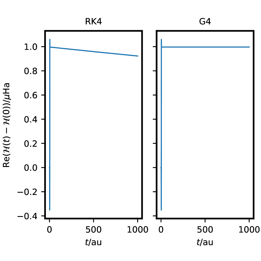
Figure 1: Total CCSD correlation energy computed as the real part of the Hamilton function ${\cal H}$ as a function of time for the RK4 and fourth-order Gauss integrators for He with the cc-pVDZ basis set and time step $h=0.1\,\text{au}$.

While the Gauss integrator maintains a constant energy after the external force has been applied, the RK4 integrator leads to loss of energy, explicitly demonstrating the benefit of applying a symplectic method. Since CCSD is equivalent to FCI for this system, the Hamilton function should be manifestly real, at least within exact arithmetic.

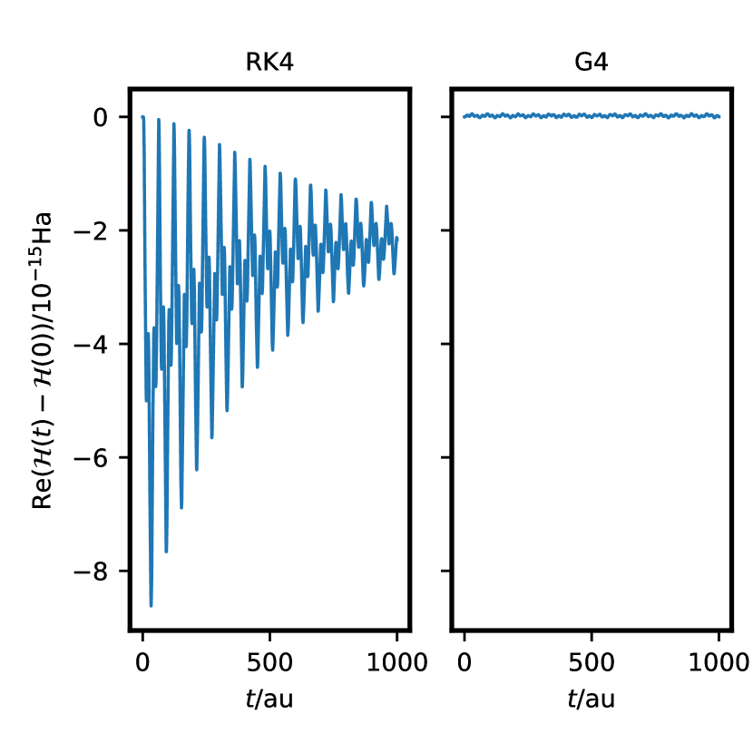
Figure 2: The imaginary part of the CCSD Hamilton function ${\cal H}$ as a function of time for the RK4 and fourth-order Gauss integrators for He with the cc-pVDZ basis set and time step $h=0.1\,\text{au}$.

The imaginary part is indeed very small with both integrators but, as shown in Fig. 2, the RK4 integrator leads to an oscillatory imaginary part, which is about two orders of magnitude greater than that observed with the G4 integrator. The maximum absolute imaginary part of the CCSD Hamilton function is $9\cdot 10^{-15}\,\text{Ha}$ with the RK4 integrator compared with $5\cdot 10^{-17}\,\text{Ha}$ with the G4 integrator. In order to test whether these values are meaningful and not merely numerical noise, we investigate the effect of increasing and decreasing the time step and find that the ratio of about $100$ persists: Doubling the time step to $h=0.2\,\text{au}$, the maximum absolute imaginary part of the CCSD Hamilton function increases to $7\cdot 10^{-14}\,\text{Ha}$ with the RK4 integrator and $5\cdot 10^{-16}\,\text{Ha}$ with the G4 integrator. Halving the time step to $h=0.05\,\text{au}$, the maximum absolute imaginary part of the CCSD Hamilton function decreases to $3\cdot 10^{-16}\,\text{Ha}$ with the RK4 integrator and $3\cdot 10^{-18}\,\text{Ha}$ with the G4 integrator.

While tiny, we speculate that the imaginary parts may become significantly greater for the larger time steps required for realistic simulations on larger molecules, and that a symplectic method will outperform RK4 in this respect. For example, running the same simulation for the slightly larger Be atom with the cc-pVDZ basis, the maximum absolute imaginary part of the CCSD Hamilton function increases to $2\cdot 10^{-14}\,\text{Ha}$ with the RK4 integrator and $2\cdot 10^{-16}\,\text{Ha}$ with the G4 integrator; see also Ref. Pigg et al., 2012.

We stress that although symplecticity is highly desirable, the RK4 integrator may still produce sufficiently accurate results for properties other than the energy. For example, computing the lowest-lying singlet excitation energy ($1\text{s}\rightarrow 2\text{p}$ transition) through the Fast Fourier Transform (FFT) of the dipole moment induced by the electric-field kick yields the same result, $2.871\,\text{Ha}$, for He with the RK4 and G4 integrators. This agrees with the excitation energy obtained from EOM-CCSD (diagonalization), $2.874\,\text{Ha}$, to within the frequency resolution of the FFT, which is $0.006\,\text{Ha}$ in this case. Moreover, the energy drift of the RK4 integrator may be minimized by reducing the time step, albeit at the expense of computational cost due to the increasing number of $f$ evaluations required.

III.3 Computational performance of Gauss integrators

We now turn to the efficiency of the Gauss integrator as measured by the number of $f$ evaluations per time step, which should be compared with the four evaluations per time step required by the RK4 integrator. As discussed above, the crucial parameter here is the initial guess for the fixed-point iterations. We use the same test system as in the previous section, i.e., the He atom with the cc-pVDZ basis set exposed to the same electric-field kick. The number of $f$ evaluations per time step is measured for simulations of duration $20\,\text{au}$.

Figure 3 shows the number of $f$ evaluations per time step required by the Gauss integrators of order $4$, $6$, $8$, and $10$ as functions of $h^{-1}$, the number of steps taken to propagate through one atomic unit of time.

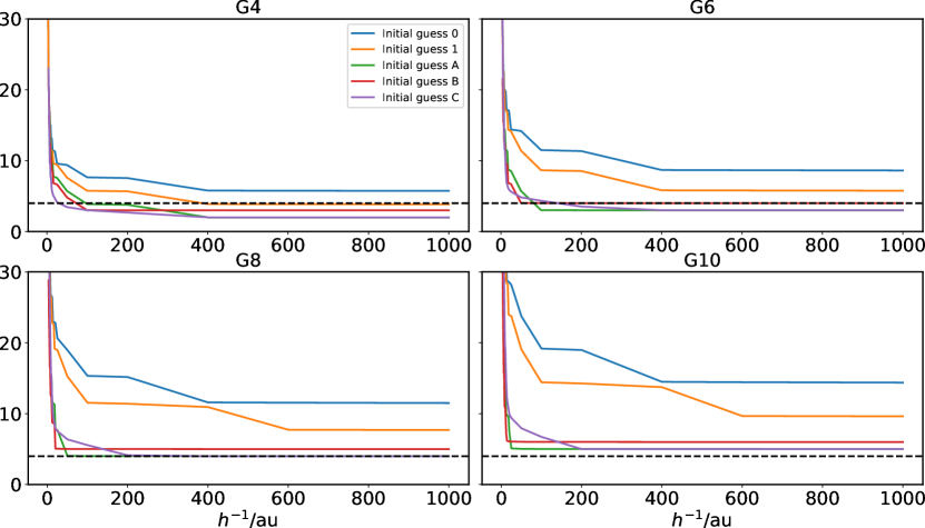
Figure 3: Number of $f$ evaluations per time step as a function of the inverse time step size for Gauss integrators of orders $4,6,8,10$ for He with the cc-pVDZ basis set and simulation time $20\,\text{au}$. The horizontal dashed lines mark the number (four) of $f$ evaluations per time step required by the RK4 integrator.

As discussed above, the number of $f$ evaluations per time step depends on the number of iterations required to converge the fixed-point iterations and thus depends crucially on the initial guess for these iterations. It is immediately clear from Fig. 3 that all five initial guesses perform poorly with large time steps. Although the performance is likely to improve by application of convergence acceleration techniques, it will be difficult to compete with the RK4 integrator with larger time steps. On the other hand, this regime is where the symplecticity problems of the RK4 integrator are most pronounced and the additional cost of the Gauss integrators may be time well spent. As the time step is decreased, the number of $f$ evaluations decrease dramatically with the more advanced initial guesses A, B, and C. With sufficiently small time steps, the implicit Gauss integrators require exactly $s$ (for initial guesses A and C) or $s+1$ (for initial guess B) $f$ evaluations per time step, meaning that they are effectively equivalent to explicit integrators in terms of computational effort. Remarkably, for smaller time steps and using initial guesses A or C, the Gauss integrators up to and including order 8 are at least as fast as the RK4 integrator with the same time step.

These features are also evident from Fig. 4, which shows the total number of $f$ evaluations as a function of the order of the Gauss integrator for the three initial guesses A, B, C.

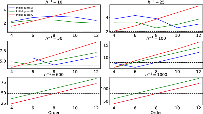
Figure 4: Total number of $f$ evaluations (in thousands) as a function of the order of the Gauss integrator, plotted as lines for visual aid, for He with the cc-pVDZ basis set and simulation time $20\,\text{au}$. The horizontal dashed lines mark the number of $f$ evaluations used by the RK4 integrator with the indicated time step. In the last two plots, the lines for initial guesses A and C coincide.

Note, in particular, that initial guesses A and B may be more efficient at higher orders for larger steps, since $s$ (half the order of the integrator), also determines the order of the initial guess. Hairer, Lubich, and Wanner (2006) With $h=0.1\,\text{au}$, for example, initial guess B requires slightly fewer $f$ evaluations at order $12$ than at order $4$, and with $h=0.02\,\text{au}$, initial guess A reduces the effort by about $1/3$ at order $8$ compared with order $4$, making the G8 integrator virtually indistinguishable from the RK4 integrator in terms of computer time.

At any rate, the total number of $f$ evaluations renders time-dependent CC simulations a formidable computational task compared with ground-state and response calculations, which require on the order of $10$–$100$ evaluations. Consequently, the application scope of time-dependent CC theory must be the study of processes where the quantum dynamics is essential and/or where time-dependent perturbation theory breaks down.

III.4 Autocorrelation functions

We now investigate the autocorrelation function, Eq. (18), as a tool for extracting information about stationary states in time-dependent CC simulations. To this end, we first expose the system to a laser pulse of the form (33) with the sinusoidal envelope (34) from time $t=0$ to time $t=t_{1}$. Subsequently, we record the induced dipole moment and the autocorrelation function $A(t_{1},t)$ for $t>t_{1}$.

We first expose the He atom to a laser pulse defined by Eqs. (33) and (34) with the parameters $\omega=2.8735643\,\text{au}$, $t_{0}=0\,\text{au}$, and $t_{d}=5\,\text{au}$. The carrier frequency corresponds to the lowest-lying EOM-CCSD/cc-pVDZ electric-dipole allowed transition from the ground state of He and the electric field is linearly polarized along the $z$-axis. We then simulate the evolution of the electronic system in two steps, first in the presence of the laser pulse from $t=t_{0}=0\,\text{au}$ to $t=t_{1}=t_{d}=5\,\text{au}$ and then in the absence of a field from $t=t_{1}$ to $t=t_{1}+5000$ at the CCSD/cc-pVDZ level using the G6 integrator with time step $h=0.01\,\text{au}$. The resulting frequency resolution is $1.26\cdot 10^{-3}\,\text{au}$. This procedure is repeated with varying electric-field strengths ranging from $10^{-3}\,\text{au}$ to $10\,\text{au}$, with corresponding ponderomotive energiesKrausz and Ivanov (2009) $U_{\text{p}}=\boldsymbol{E}^{2}/4\omega^{2}$ in the range from $10^{-8}\,\text{au}$ to $3\,\text{au}$. The field strengths thus range from very weak to slightly above the perturbation limit, which is taken to be the line in an intensity–frequency plot where the ponderomotive energy is equal to the carrier frequency. We note in passing that none of the field strengths are near the relativistic limit.

The ground-state probability for He during the laser pulse is plotted as a function of time in Figure 5 for each field strength.

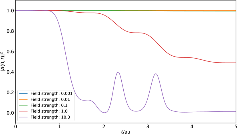
Figure 5: Evolution of the ground-state probability during the laser pulse for the He atom at different field strengths computed at the time-dependent CCSD/cc-pVDZ level of theory.

These curves are identical to the probabilities computed with regular time-dependent FCI using the same integrator, validating the time-dependent CCSD implementation. The final ground-state probabilities (at $t=5\,\text{au}$), in order of increasing field strength, are $99.9999\,\%$, $99.9932\,\%$, $99.3213\,\%$, $48.8647\,\%$, and $1.3835\,\%$, showing that one of the fundamental assumptions of time-dependent perturbation theory—the ground-state probability must remain close to unity—is valid for field strengths up to at least $10^{-1}\,\text{au}$ in this case. The final state with field strength $10\,\text{au}$, on the other hand, is nearly orthogonal to the ground state. At this field strength we also note that induced emission causes partial “revival” of the ground state while the laser pulse is on. As argued above, Fourier transformation of the autocorrelation function $A(t_{1},t)$ ($t_{1}=5\,\text{au}$) provides information of about the populated excited energy levels. This information is plotted in Fig. 6 superimposed on the energy levels obtained from EOM-CCSD.

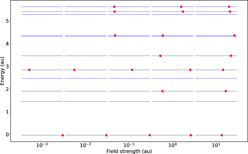
Figure 6: Unrestricted EOM-CCSD energy levels of He with the cc-pVDZ basis. Circles indicate the energy levels contributing to the CC state as detected by FFT of the autocorrelation function $A(t_{1},t)$ at the given field strength. The horizontal position of each circle indicates the relative and normalized weight of that level obtained from the peak intensities of the FFT. The weight scale is logarithmic and extends from $10^{-5}$ (left edge of each horizontal line) to $1$ (right edge of each horizontal line).

The weights plotted in this figure are indicative of, but not identical to, the probabilities associated with each energy level, since the former are computed from renormalized relative peak intensities of the FFT of the signal. At the lowest field strengths only one excited level is populated and, indeed, only the $0\to 4$ transition is observed in the dipole spectrum computed by FFT of the induced dipole moment at $t\in[5,5005]\,\text{au}$. (The states are numbered according to increasing energy.) Higher-lying levels become weakly populated at field strength $0.1\,\text{au}$ and the dipole spectrum now contains very weak lines that can be assigned to transitions between excited states (in order of decreasing intensity: $4$ and $10$, $4$ and $9$, $7$ and $10$, $7$ and $9$). Going to field strength $1\,\text{au}$, the dipole-forbidden (i.e., no direct electric-dipole transition from the ground state) level $2$ becomes populated and the weight of level $4$ rivals that of the ground state, which is still the most probable stationary state contributing to the CC state and the transition $0\to 4$ remains the most intense in the dipole spectrum. This is no longer the case at field strength $10\,\text{au}$ where the ground state has become the least likely, as one might also suspect from its low probability $|A(0,t_{1})|^{2}=1.3835\,\%$. The CCSD dipole spectrum at field strength $10\,\text{au}$ is plotted in Fig. 7.

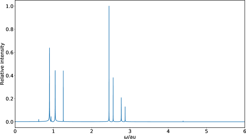
Figure 7: Dipole spectrum of He at field strength $10\,\text{au}$ computed at the time-dependent CCSD/cc-pVDZ level of theory.

The most intense line corresponds to the transition $2\to 7$ and the transition $0\to 4$, which is the most intense line at the lower field strengths, has dropped to a relative intensity of $0.13$.

Running the same simulations for the Be atom with the cc-pVDZ basis set at field strengths ranging from $10^{-3}\,\text{au}$ to $0.3\,\text{au}$ and carrier frequency $\omega=0.2068175\,\text{au}$, which corresponds to the lowest-lying EOM-CCSD/cc-pVDZ electric-dipole allowed transition from the ground state, leads to the ground-state probabilities during the laser pulse plotted in Fig. 8.

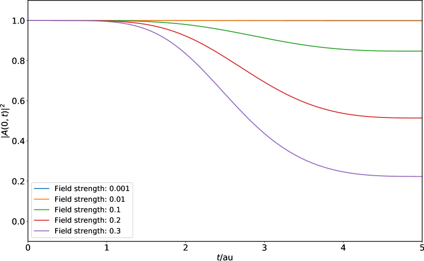
Figure 8: Evolution of the ground-state probability during the laser pulse for the Be atom at different field strengths computed at the time-dependent CCSD/cc-pVDZ level of theory.

Despite the lower field strengths compared with the He case discussed above, the lower carrier frequency ensures comparable ponderomotive energies ranging from $5.84\cdot 10^{-6}\,\text{au}$ to $0.53\,\text{au}$, the latter being well above the perturbative limit. The lower carrier frequency also means that the laser pulse is less oscillatory, leading to more monotonic decay of the ground-state probability. The final probabilities are $99.998\,\%$, $99.835\,\%$, $84.728\,\%$, $51.440\,\%$, and $22.331\,\%$, clearly indicating the deviation from a perturbative treatment at the greater field strengths. Running the same simulation at the time-dependent FCI/cc-pVDZ level with field strength $0.3\,\text{au}$ yields a ground-state probability curve virtually indistuinguishable from the CCSD one in Fig. 8: the root-mean-square deviation between the curves is merely $3\cdot 10^{-4}$ with a maximum deviation of $4\cdot 10^{-4}$.

The contributing energy levels computed by FFT of the autocorrelation function $A(t_{1},t)$ are superimposed on the EOM-CCSD levels in Fig. 9.

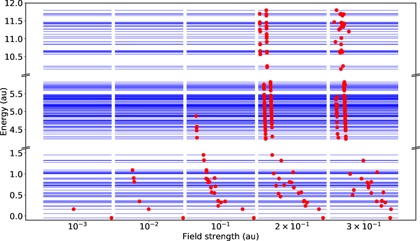
Figure 9: Unrestricted EOM-CCSD energy levels of Be with the cc-pVDZ basis. Circles indicate the energy levels contributing to the CC state as detected by FFT of the autocorrelation function $A(t_{1},t)$ at the given field strength. The horizontal position of each circle indicates the relative and normalized weight of that level obtained from the peak intensities of the FFT. The weight scale is logarithmic and extends from $10^{-5}$ (left edge of each horizontal line) to $1$ (right edge of each horizontal line).

At field strength $10^{-3}\,\text{au}$ the only contributing excited state is the lowest-lying dipole-allowed state that can be reached from the ground state. Five excited states contribute at field strength $10^{-2}\,\text{au}$ and analysis of the dipole spectrum reveals that all five states are reached by direct excitation from the ground state. Transitions between excited states appear at field strength $0.1\,\text{au}$, although specific assignment of each line in the dipole spectrum is made difficult by the limited frequency resolution (caused by finite simulation time) combined with the closeness of the excited states. More than $70\,\%$ of the states contribute at field strengths $0.2\,\text{au}$ and $0.3\,\text{au}$, albeit mostly with very low weight. At field strength $0.3\,\text{au}$ the ground state is no longer the most probable state and several excited levels have comparable weights. The dipole spectrum, shown in Fig. 10 along with the spectrum computed at the FCI level, clearly displays several transitions between close-lying excited states.

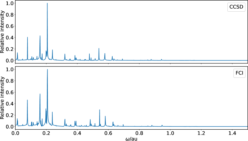
Figure 10: Dipole spectrum of Be at field strength $0.3\,\text{au}$ computed at the time-dependent CCSD/cc-pVDZ and FCI/cc-pVDZ levels of theory.

The most intense line peaks at $0.206\,\text{au}$ and corresponds to the $0\to 2$ transition, which is the lowest-lying electric-dipole allowed transition from the ground state. Aside from minor differences in relative intensities, the CCSD spectrum agrees very well with the FCI spectrum, increasing the confidence in our time-dependent CCSD implementation.

Equation (19) offers an alternative assessment of the sufficiency of a perturbative treatment. Table 1 reports the root-mean-square deviation from $1$ and $0$ of the real and imaginary parts of $\tilde{A}(t_{1},t)=\exp(\text{i}E_{0}(t-t_{1}))A(t_{1},t)$, respectively, for He and Be.

Table 1: Root-mean-square deviation of $\tilde{A}(t_{1},t)=\exp(\text{i}E_{0}(t-t_{1}))A(t_{1},t)$ computed at the time-dependent CCSD/cc-pVDZ level of theory for $t_{1}=5\,\text{au},t\in[5,5005]\,\text{au}$.

He
Field strength (au)	$10^{-3}$	$10^{-2}$	$10^{-1}$	$10^{0}$	$10^{1}$
Re$[\tilde{A}(t_{1},t)]$	$8\cdot 10^{-7}$	$8\cdot 10^{-5}$	$8\cdot 10^{-3}$	$6\cdot 10^{-1}$	$1$
Im$[\tilde{A}(t_{1},t)]$	$1\cdot 10^{-4}$	$1\cdot 10^{-4}$	$5\cdot 10^{-3}$	$3\cdot 10^{-1}$	$4\cdot 10^{-1}$
Be
Field strength (au)	$10^{-3}$	$10^{-2}$	$10^{-1}$	$2\cdot 10^{-1}$	$3\cdot 10^{-1}$
Re$[\tilde{A}(t_{1},t)]$	$2\cdot 10^{-5}$	$2\cdot 10^{-3}$	$2\cdot 10^{-1}$	$5\cdot 10^{-1}$	$8\cdot 10^{-1}$
Im$[\tilde{A}(t_{1},t)]$	$4\cdot 10^{-4}$	$1\cdot 10^{-3}$	$1\cdot 10^{-1}$	$2\cdot 10^{-1}$	$2\cdot 10^{-1}$

Overall, the root-mean-square deviations agree with the results above. For He, field strengths $1\,\text{au}$ and $10\,\text{au}$ are clearly non-perturbative, and for Be, field strengths $0.1$–$0.3\,\text{au}$ are non-perturbative.

III.5 Very strong fields

Increasing the field strength beyond those of the previous section poses a numerical challenge to the CCSD model, even for the He atom where it is formally equivalent to FCI. This can be understood from the following simple qualitative analysis. As the field strength is increased, the ground-state probability tends to zero and since the ground state of He (and Be) is vastly dominated by the HF reference determinant, we may take this to mean that the state of the system is a superposition of excited determinants. In the limit of untruncated cluster operators, $|\Psi\rangle$ and $\langle\tilde{\Psi}|$ are proportional to the FCI state and its conjugate, respectively. As the FCI coefficient $C_{0}$ of the HF determinant approaches zero, the amplitudes of the CCSD state must behave in a rather extreme fashion:

$$C_{0}=\langle\Psi|\Psi\rangle^{-1/2}e^{iy}e^{x}\to 0,$$ (36)

$$C_{0}^{*}=\langle\tilde{\Psi}|\tilde{\Psi}\rangle^{-1/2}e^{-iy}e^{-x}$$

$$\qquad\times\left(1-\lambda_{1}\tau_{1}-\lambda_{2}\tau_{2}+\frac{1}{2}\lambda_{2}\tau_{1}^{2})\right)\to 0,$$ (37)

where $\lambda_{i},\tau_{i},i=1,2$, collectively denote the suitable singles and doubles amplitudes, and

$$x(t)=\operatorname{Re}\tau_{0}(t)=\operatorname{Im}\int_{0}^{t}\langle\Phi_{0}|e^{-T(t^{\prime})}H(t^{\prime})e^{T(t^{\prime})}|\Phi_{0}\rangle\,\text{d}t^{\prime},$$ (38)

$$y(t)=\operatorname{Im}\tau_{0}(t)=-\operatorname{Re}\int_{0}^{t}\langle\Phi_{0}|e^{-T(t^{\prime})}H(t^{\prime})e^{T(t^{\prime})}|\Phi_{0}\rangle\,\text{d}t^{\prime}.$$ (39)

Evidently, the absolute value of the $\tau$ amplitudes must increase to make $\langle\Psi|\Psi\rangle$ and $\langle\tilde{\Psi}|\tilde{\Psi}\rangle$ as large as possible while maintaining the absolute value of $x$ low enough to overcome the exponential increase of either $\exp(x)$ or $\exp(-x)$. By the same token, the $\lambda$ amplitudes must not increase too much. This represents a delicate numerical challenge.

An example is presented in Fig. 11 for the He atom when the field strength is increased to $100\,\text{au}$—all other parameters of the sinusoidal laser pulse and the G6 integrator are the same as in the previous section. This corresponds to a ponderomotive energy of $303\,\text{au}$, which is equivalent to about $105$ photons at the carrier frequency.

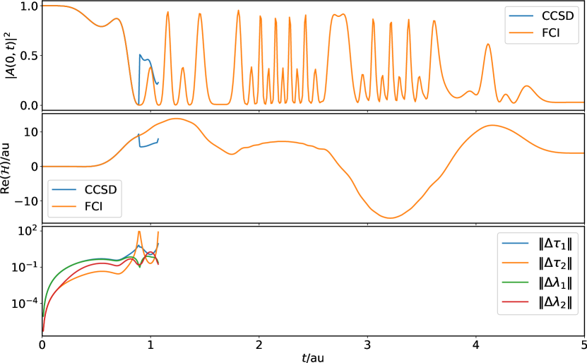
Figure 11: Time-dependent CCSD and FCI simulations of He with the cc-pVDZ basis exposed to a laser pulse of field strength $100\,\text{au}$ and carrier frequency $\omega=2.8735643\,\text{au}$. Top panel: ground-state probability. Middle panel: real part of the Hamilton function. Bottom panel: norm of the change in amplitudes relative to the initial (ground) state.

The CCSD ground-state probability and Hamilton function are indistinguishable from the FCI simulation until $t=0.88\,\text{au}$; at $t=1.07\,\text{au}$ the CCSD simulation fails due to numerical instability. The ground-state probability in this time interval drops to about $0.2\,\%$ accompanied by rapid increase of (the norm of) the amplitudes, especially the $\tau$ amplitudes, which causes numerical instability in double-precision arithmetic while solving Eq. (27).

As shown in Fig. 12, the same problem appears in the simulation of the Be atom exposed to a laser pulse of $1\,\text{au}$, correponding to a ponderomotive energy of $5.84\,\text{au}$ (roughly $28$ photons at the carrier frequency).

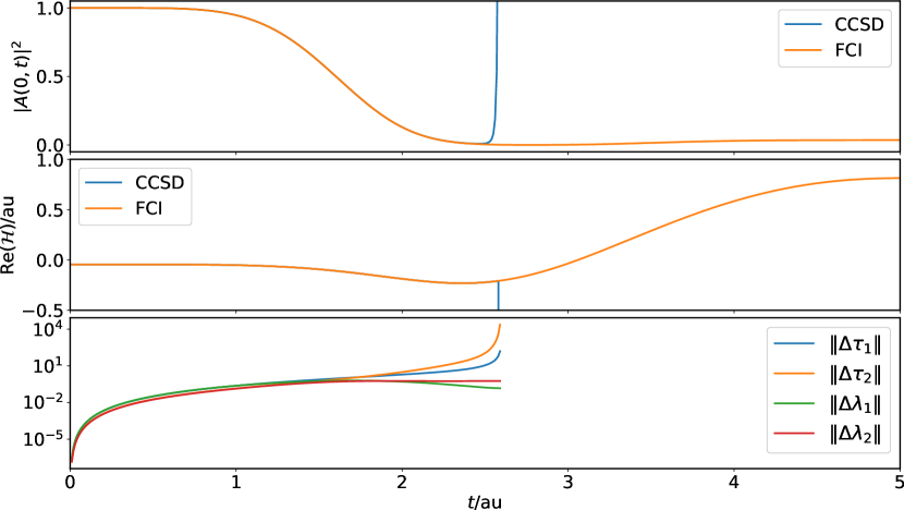
Figure 12: Time-dependent CCSD and FCI simulations of Be with the cc-pVDZ basis exposed to a laser pulse of field strength $1\,\text{au}$ and carrier frequency $\omega=0.2068175\,\text{au}$. Top panel: ground-state probability. Middle panel: real part of the Hamilton function. Bottom panel: norm of the change in amplitudes relative to the initial (ground) state.

Again, the numerical instability can be traced to rapid changes in the amplitudes relative to the ground state as the ground-state probability approaches zero. In this case, CCSD is an approximation and both the ground-state probility and Hamilton function differ from the FCI results, although the differences are too small to be visible on the scale of the plots in Fig. 12.

Such numerical instabilities may also be encountered within the CCSD model at less intense field strengths, as illustrated by CCSD and FCI simulations of the Be atom with a field strength of $0.5\,\text{au}$ presented in Fig. 13, which shows results for $t>5\,\text{au}$—i.e., after the laser pulse has been turned off. At $t=5\,\text{au}$ the amplitude norms are roughly $3$ and $19$ for $\tau_{1}$ and $\tau_{2}$, and $0.3$ and $0.6$ for $\lambda_{1}$ and $\lambda_{2}$. The norm of the change in amplitudes reported in Fig. 13 are measured relative to these.

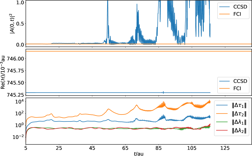
Figure 13: Time-dependent CCSD and FCI simulations of Be with the cc-pVDZ basis exposed to a laser pulse of field strength $0.5\,\text{au}$ and carrier frequency $\omega=0.2068175\,\text{au}$. Top panel: ground-state probability. Middle panel: real part of the Hamilton function. Bottom panel: norm of the change in amplitudes relative to the state at $t=5\,\text{au}$.

In agreement with the FCI value of $1.6\%$ at $t=5\,\text{au}$, the CCSD ground-state probability is $1.7\%$. At times $t>5\,\text{au}$ both the ground-state probability and the Hamilton function should remain constant. This is indeed the case for the FCI simulation but the CCSD method fails spectacularly for the ground-state probability at $t\gtrapprox 20\,\text{au}$. This is caused by numerical noise accumulating in the amplitudes, eventually causing the simulation to fail. Note, however, that the CCSD Hamilton function remains almost constant throughout, except for a sub-millihartree oscillation at $t\approx 90\,\text{au}$. This feature can be ascribed to the symplecticity of the Gauss integrator.

One might speculate that this is an effect of a too small basis set, but repeating the simulations with the aug-cc-pVDZ and cc-pVTZ basis sets leads to essentially identical behavior for Be with field strength $0.5\,\text{au}$. No problems are observed with a minimal basis set, however, indicating that increasing the basis set further, for example by inclusion of low-lying continuum functions to support ionization processes, is unlikely to resolve the problem.

IV Concluding remarks

In this study we have

• exploited the Hamiltonian structure of time-dependent CC theory to propose the Gauss integrator as a stable algorithm for solving the time-dependent CC equations,

• proposed autocorrelation functions based on an indefinite inner product for analyzing the time-dependent CC state,

• presented a pilot implementation and validated it through simulations of the He and Be atoms in short laser pulses with increasing intensity, comparing with results obtained with the time-dependent FCI method, and

• observed that the CCSD approach fails for very strong laser pulses due to numerically intractable increase in the $\tau$ amplitudes as the ground-state probability approaches zero.

We stress that the CCSD failure persists in the FCI limit even if, mathematically, the combined exponential ($\tau$) and linear ($\lambda$) parametrization should be sufficiently flexible to fully describe the electron dynamics. While it may be possible to devise an integrator with sufficient numerical stability, possibly in conjunction with the use of even smaller time steps, the most likely solution is to allow the underlying orbitals to participate in the correlated electron dynamics in a manner similar to the approaches of Kvaal Kvaal (2012) or Sato et al. Sato et al. (2018) but in such a way that the FCI limit is recovered for more than two electrons. Köhn and Olsen (2005); Myhre (2018); Kvaal (2012) A properly constructed moving reference determinant would capture the main effects of the laser pulse (which is represented by a one-electron operator), ensuring a significant overlap with the FCI wave function and thus leading to well-behaved amplitudes.