Low energy neutrinos from stopped muons in the Earth

Abstract

We explore the low energy neutrinos from stopped cosmic ray muons in the Earth. Based on the muon intensity at the sea level and the muon energy loss rate, the depth distributions of stopped muons in the rock and sea water can be derived. Then we estimate the $\mu^{-}$ decay and nuclear capture probabilities in the rock. Finally, we calculate the low energy neutrino fluxes and find that they depend heavily on the detector depth $d$. For $d=1000$ m, the $\nu_{e}$, $\bar{\nu}_{e}$, $\nu_{\mu}$ and $\bar{\nu}_{\mu}$ fluxes in the range of 13 MeV $\leq E_{\nu}\leq$ 53 MeV are averagely $10.8\%$, $6.3\%$, $3.7\%$ and $6.2\%$ of the corresponding atmospheric neutrino fluxes, respectively. The above results will be increased by a factor of 1.4 if the detector depth $d<30$ m. In addition, we find that most neutrinos come from the region within 200 km and the near horizontal direction, and the $\bar{\nu}_{e}$ flux depends on the local rock and water distributions.

I Introduction

Atmospheric neutrinos are a very important neutrino source to study the neutrino oscillation physics. In 1998, the Super-Kamiokande (Super-K) experiment reported the first evidence of neutrino oscillations based on a zenith angle dependent deficit of atmospheric muon neutrinos Fukuda:1998mi . Atmospheric neutrinos are produced in the Earth’s atmosphere as a result of cosmic ray interactions and the weak decays of secondary mesons, in particular pions and kaons Honda:2006qj . At the same time, a large amount of muons are also produced and some of them can penetrate the rock and sea water of Earth’s surface to significant depths. These penetrating muons are the important background source for some underground experiments Li:2014sea . It is well known that these muons will finally stop in the Earth and then produce the low energy neutrinos through decay or nuclear capture Measday:2001yr . However, these neutrinos are not included in the previous literatures Gaisser:1988ar ; Honda:1995hz ; Battistoni:2005pd . Here we shall focus on these neglected neutrinos from stopped muons in the Earth.

Muons are the most numerous charged particles at sea level PDG . After losing energy by ionization and radiative processes, the stopped $\mu^{+}$ in the rock and sea water will generate two low energy neutrinos $\nu_{e}$ and $\bar{\nu}_{\mu}$ ($E_{\nu}\leq 53$ MeV) through $\mu^{+}\rightarrow e^{+}+\nu_{e}+\bar{\nu}_{\mu}$. Unlike $\mu^{+}$, the stopped $\mu^{-}$ may undergo either decay or capture by the nucleus Measday:2001yr . In the nuclear capture case, a stopped $\mu^{-}$ can only produce a neutrino $\nu_{\mu}$ with energy less than the muon mass. These low energy neutrinos will be the background source in the searches of some relevant physics, such as diffuse supernova relic neutrinos Ando:2004hc ; An:2015jdp , dark matter annihilation in the Sun Rott:2012qb and our galaxy PalomaresRuiz:2007eu , solar neutrino conversion Collaboration:2011jza , and proton decays catalyzed by GUT monopoles in the Sun Ueno:2012md . So it is necessary for us to investigate the low energy neutrinos induced by stopped muons in the Earth.

In this paper, we shall calculate the neutrino fluxes from stopped cosmic ray muons in the Earth. In Sec. II, the stopped $\mu^{\pm}$ distributions in the rock and sea water will be given in terms of the muon intensity at the sea level and the muon energy loss rate. Sec. III is devoted to the $\bar{\nu}_{e}$ and $\nu_{\mu}$ energy spectra from a stopped $\mu^{-}$. Based on the atomic capture and nuclear capture abilities of 10 dominant elements in the upper continental crust, we estimate the $\mu^{-}$ decay and nuclear capture probabilities in the rock and sea water. In Sec. IV, we numerically calculate the low energy neutrino fluxes according to the stopped $\mu^{\pm}$ distributions and the $\mu^{-}$ decay probability, and discuss their features. In addition, an approximation formula to compute the neutrino fluxes has also been presented. Finally, our conclusions will be given in Sec. V.

II Distributions of stopped muons

Muons are the most numerous charged particles at sea level PDG . For the energy and angular distribution of cosmic ray muons at the sea level, we use the following parameterization Reyna:2006pv

$$I(p_{\mu},\theta)=I_{\rm v}(\xi)\,\cos^{3}\theta\;\;{\rm for}\;\;p_{\mu}>1{\rm GeV}\,,$$ (1)

with $\xi=p_{\mu}\cos\theta$ and $\theta$ is the zenith angle. The vertical muon intensity is given by

$$I_{\rm v}(p_{\mu})=c_{1}p_{\mu}^{-(c_{2}+c_{3}\log p_{\mu}+c_{4}\log^{2}p_{\mu}+c_{5}\log^{3}p_{\mu})}\,,$$ (2)

where $c_{1}=0.00253\,{\rm cm^{-2}s^{-1}sr^{-1}GeV^{-1}}$, $c_{2}=0.2455$, $c_{3}=1.288$, $c_{4}=-0.2555$ and $c_{5}=0.0209$. It is found that Eq. (1) is valid for all zenith angles and the muon momentum $p_{\mu}>1$ GeV Reyna:2006pv . For $p_{\mu}\leq 1$ GeV, the muon energy spectrum is almost flat and the corresponding angular distribution is steeper than $\cos^{2}\theta$ PDG . Therefore we assume

$$I(p_{\mu},\theta)=0.00389\cos^{3}\theta\;\;{\rm for}\;\;p_{\mu}\leq 1{\rm GeV}\,,$$ (3)

in the units of ${\rm cm^{-2}s^{-1}sr^{-1}GeV^{-1}}$. In terms of of Eqs. (1)-(3), the total muon flux for a horizontal detector can be derived from

$$J_{\mu}=2\pi\int I(p_{\mu},\theta)\cos\theta\;d\cos\theta\,dp_{\mu}=1\,{\rm cm^{-2}\,min^{-1}}\;,$$ (4)

which is familiar to experimentalists for horizontal detectors PDG . The muons with $p_{\mu}>1{\rm GeV}$ make a $71\%$ contribution to $J_{\mu}$. With the help of the muon charge ratio in Fig. 6 of Ref. Naumov:2002dm , we calculate the $\mu^{+}$ flux $J_{\mu^{+}}=0.0093\,{\rm cm^{-2}s^{-1}}$ and the $\mu^{-}$ flux $J_{\mu^{-}}=0.00737\,{\rm cm^{-2}s^{-1}}$, and the corresponding muon charge ratio $J_{\mu^{+}}/J_{\mu^{-}}=1.26$.

The long-lived muons can penetrate the rock and sea water of the Earth’s surface to significant depths. The muon range $X(p_{\mu})$ in the standard rock and water may be found in Ref. Groom:2001kq . Then one can easily get the stop depth $x=X(p_{\mu})\cos\theta$ for a muon with the momentum $p_{\mu}$ and incidence zenith angle $\theta$ at the sea level. Based on the muon distribution $I(p_{\mu},\theta)$, muon charge ratio Naumov:2002dm and muon range $X(p_{\mu})$ Groom:2001kq , we calculate the $\mu^{\pm}$ stop rate per unit volume $S_{\mu^{\pm}}(x)$ in the standard rock and water. In Fig. 1, the $\mu^{\pm}$ stop rate $S_{\mu^{\pm}}(x)$ and the charge ratio of stopped muons $S_{\mu^{+}}/S_{\mu^{-}}$ as a function of stop depth $x$ have been plotted. It is clear that the depth $x$ of most stopped muons is less than 30 m.

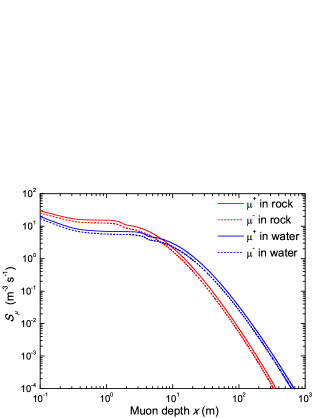
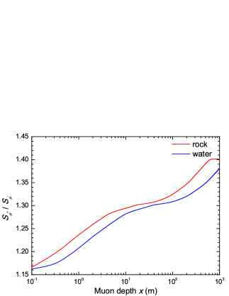
Figure 1: The muon stop rate per unit volume $S_{\mu^{\pm}}$ (left) and the charge ratio of stopped muons $S_{\mu^{+}}/S_{\mu^{-}}$ (right) as a function of stop depth $x$ in the standard rock and water.

III Neutrino energy spectra from a stopped muon

It is well known that a stopped $\mu^{+}$ will quickly decay into a positron and two neutrinos through $\mu^{+}\rightarrow e^{+}+\nu_{e}+\bar{\nu}_{\mu}$. The $\nu_{e}$ and $\bar{\nu}_{\mu}$ energy spectra (normalized to 1) can be written as Coloma:2017egw

$$f_{\nu_{e}} = \frac{192}{m_{\mu}}\left[\left(\frac{E_{\nu}}{m_{\mu}}\right)^{2}\left(\frac{1}{2}-\frac{E_{\nu}}{m_{\mu}}\right)\right]\;,$$ (5)

$$f_{\bar{\nu}_{\mu}} = \frac{64}{m_{\mu}}\left[\left(\frac{E_{\nu}}{m_{\mu}}\right)^{2}\left(\frac{3}{4}-\frac{E_{\nu}}{m_{\mu}}\right)\right]\;,$$ (6)

where $m_{\mu}$ is the muon mass and $E_{\nu}\leq m_{\mu}/2$. Unlike $\mu^{+}$, a stopped $\mu^{-}$ can not only decay $\mu^{-}\rightarrow e^{-}+\bar{\nu}_{e}+\nu_{\mu}$, but also be captured by nucleus and produce a neutrino $\nu_{\mu}$ with $E_{\nu}<m_{\mu}$, such as $\mu^{-}+^{16}{\rm O}\rightarrow^{16}{\rm N}^{\ast}+\nu_{\mu}$. In fact, the stopped $\mu^{-}$ will be quickly attached to an atom and form a muonic atom (Atomic capture) Measday:2001yr when it stops in the rock or sea water. Then it cascades down to the lowest 1$s$ level in a time-scale of the order of $10^{-13}$ s through emitting Auger electrons and muonic X-rays. In the following time, the bounded $\mu^{-}$ in a muonic atom has only two choices, to decay or to capture on the nucleus (Nuclear capture) Measday:2001yr .

In order to estimate the $\mu^{-}$ decay and nuclear capture probabilities, we should firstly consider the relative abilities of atomic capture for different elements in the rock. Egidy and Hartmann VonEgidy:1982pe find a semi-empirical approach and give the average atomic capture probability $P(Z)$ for 65 elements, normalized to 1 for ${}^{16}{\rm O}$. For the rock chemical composition, we take the upper continental crust data from Ref. Rundick . Then the mass and number percentages of 10 dominant elements in the upper continental crust have been calculated and listed in Table 1. Considering the corresponding atomic capture probability $P(Z)$, we derive the atomic capture percentages of 10 elements as shown in the fifth column of Table 1. It is worthwhile to stress that the water is a ${}^{16}{\rm O}$ target since $\mu^{-}p$ can easily penetrate nearby ${}^{16}{\rm O}$ atoms Measday:2001yr .

Elements	Mass ($\%$)	Number ($\%$)	$P(Z)$	Atomic capture ($\%$)	$\tau_{\mu^{-}}$ (ns)	Huff factor	$D_{\mu^{-}}$ ($\%$)
O	47.51	62.13	1.00	60.26	1795.4	0.998	81.56
Si	31.13	23.89	0.84	19.46	756	0.992	34.14
Al	8.15	3.91	0.76	2.88	864	0.993	39.05
Fe	3.92	2.27	3.28	7.21	206	0.975	9.14
Ca	2.57	2.07	1.90	3.81	332.7	0.985	14.92
Na	2.43	2.27	1.00	2.21	1204	0.996	54.58
K	2.32	1.28	1.54	1.91	435	0.987	19.54
Mg	1.50	1.99	0.93	1.79	1067.2	0.995	48.33
Ti	0.38	0.17	2.66	0.45	329.3	0.981	14.70
P	0.07	0.02	1.04	0.02	611.2	0.991	27.57

Table 1: The $\mu^{-}$ atomic capture percentages and decay probabilities $D_{\mu^{-}}$ in a muonic atom for 10 dominant elements of the upper continental crust Rundick . The corresponding mass and number percentages, average atomic capture probability $P(Z)$, $\mu^{-}$ mean life $\tau_{\mu^{-}}$ and Huff factor $Q$ have also been listed.

The decay rate $\Lambda_{\rm decay}$ and nuclear capture rate $\Lambda_{\rm capture}$ of the bounded $\mu^{-}$ in a muonic atom have the following relation Measday:2001yr

$$\Lambda_{\rm total}=\Lambda_{\rm capture}+Q\Lambda_{\rm decay}\,,$$ (7)

where $\Lambda_{\rm total}=1/\tau_{\mu^{-}}$, $\Lambda_{\rm decay}=1/\tau_{\mu^{+}}$, and $Q$ is the Huff factor Suzuki:1987jf . Then the $\mu^{-}$ decay probability can be easily obtained by

$$D_{\mu^{-}}=Q\frac{\Lambda_{\rm decay}}{\Lambda_{\rm total}}=Q\frac{\tau_{\mu^{-}}}{\tau_{\mu^{+}}}\,.$$ (8)

With the help of $\tau_{\mu^{+}}=2196.98$ ns PDG and the $\mu^{-}$ mean life in Ref. Suzuki:1987jf , we calculate the $\mu^{-}$ decay probabilities $D_{\mu^{-}}$ for 10 dominant elements as listed in the last column of Table 1. Combining the atomic capture percentages and the corresponding $D_{\mu^{-}}$ in Table 1, one can find that the averaged decay probability $D_{\mu^{-}}=60.65\%$ and nuclear capture probability $C_{\mu^{-}}=39.35\%$ for negative muons stopped in the rock. Since the water can be approximated as an ${}^{16}{\rm O}$ target, the $\mu^{-}$ decay and nuclear capture probabilities in the water are $D_{\mu^{-}}=81.56\%$ and $C_{\mu^{-}}=18.44\%$, respectively. For the $\bar{\nu}_{e}$ and $\nu_{\mu}$ energy spectra, we ignore the differences between the free $\mu^{-}$ decay and the bounded $\mu^{-}$ decay Measday:2001yr , and have

$$f_{\bar{\nu}_{e}} = f_{{\nu}_{e}}D_{\mu^{-}}\;,$$ (9)

$$f_{{\nu}_{\mu}} = f_{\bar{\nu}_{\mu}}D_{\mu^{-}}+\tilde{f}_{\nu_{\mu}}C_{\mu^{-}}\;,$$ (10)

where $\tilde{f}_{\nu_{\mu}}$ is the $\nu_{\mu}$ energy spectrum (normalized to 1) from the $\mu^{-}$ nuclear capture. It is found that $\tilde{f}_{\nu_{\mu}}$ is fairly similar to the $\gamma$ spectrum in the reaction of the $\pi^{-}$ capture on nucleus Measday:2001yr . Therefore we use the $\gamma$ spectrum from the ${}^{16}{\rm O}(\pi^{-},\gamma)^{16}{\rm N}^{*}$ experimental results Strassner:1979pz and require that the maximal neutrino energy only reaches 95 MeV for $\tilde{f}_{\nu_{\mu}}$, because the muon mass is 34 MeV less than that of a pion.

IV Neutrino fluxes from stopped muons

Since the produced neutrinos from stopped muons are isotropic, the neutrino differential fluxes can be written as

$$\frac{d\phi_{\nu_{i}}}{dE_{\nu}} = f_{\nu_{i}}\int S_{\mu^{\pm}}(x)\frac{2\pi(R_{\oplus}-x)^{2}\sin\vartheta}{4\pi r^{2}}d\vartheta dx\,,$$ (11)

where $R_{\oplus}=6371$ km is the Earth’s radius, and $\vartheta$ is the angle between the stopped $\mu^{\pm}$ and detector point seen from the Earth’s center. The distance between the stopped $\mu^{\pm}$ and detector is given by

$$r^{2}=(R_{\oplus}-x)^{2}+(R_{\oplus}-d)^{2}-2\cos\vartheta(R_{\oplus}-x)(R_{\oplus}-d)\,,$$ (12)

where $d$ is the detector depth. In fact, the neutrino oscillation should be considered Peres:2009xe , but it is beyond the scope of this paper. For a large neutrino detector, different detector parts will receive notably different neutrino fluxes from stopped muons within $r<100$ m. Therefore we take a virtual spherical detector with a 25 m radius for the following analysis, which will increase about $1\%$ flux for the $d<30$ m case. The integral flux $\phi_{\nu_{i}}$ can be obtained from Eq. (11). In the left panel of Fig. 2, we plot the cumulative percentage of $\phi_{\nu_{i}}$ as a function of surface distance $L=R_{\oplus}\vartheta$ for three typical detector depths in the rock case. Different flavors have almost identical results even in the water case. It is worthwhile to stress that the stopped muons within the surface distance $L=200$ km contribute $68.7\%$ and $56.1\%$ of $\phi_{\nu_{i}}$ for $d=0$ m and $d=1000$ m, respectively. In addition, one may easily find that most neutrinos come from the near horizontal direction. Since the recoil electrons can carry the directional information of incident neutrinos in the elastic scattering of neutrinos on electrons Ueno:2012md and $\nu_{e}$ has the largest cross section, we calculate the zenith angular distribution of $\nu_{e}$ integral flux in the rock case, as shown in the right panel of Fig. 2. It is found that the smaller $d$ case has the narrower peak at the horizontal direction. Note that the underground part of the virtual spherical detector contributes the $\cos\theta>0$ angular distribution for the depth of detector center $d=0$ m case. $\bar{\nu}_{e}$, ${\nu}_{\mu}$ and $\bar{\nu}_{\mu}$ have similar angular distributions even in the water case.

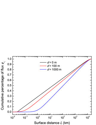
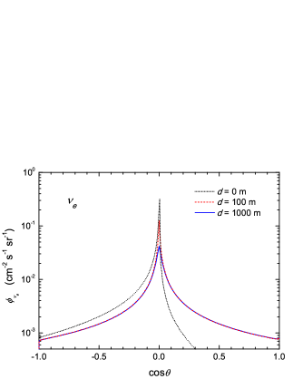
Figure 2: The cumulative percentage of the neutrino integral flux $\phi_{\nu_{i}}$ as a function of surface distance $L=R_{\oplus}\vartheta$ (left) and the $\nu_{e}$ integral flux $\phi_{\nu_{e}}$ with $E_{\nu}<53$ MeV as a function of zenith angle $\theta$ (right).

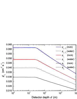
Figure 3: The neutrino flux $\phi_{\nu_{i}}$ as a function of detector depth $d$ for different neutrino flavors.

In Fig. 3, we show the neutrino integral fluxes $\phi_{\nu_{i}}$ as a function of detector depth $d$ for different flavors in the rock and water cases. It is clear that $\phi_{\nu_{i}}$ depends heavily on the detector depth $d$. For $\phi_{\nu_{e}}$, $\phi_{\bar{\nu}_{\mu}}$ and $\phi_{{\nu}_{\mu}}$, the differences between the rock and water cases are very small. However, the ${\nu}_{\mu}$ differential fluxes in the rock and water cases have obvious differences due to different values of $D_{\mu^{-}}$ and $C_{\mu^{-}}$ in Eq. (10). Note that $\phi_{\bar{\nu}_{e}}$ in the water case is larger than that in the rock case because of the larger $D_{\mu^{-}}$ in the water case. Therefore, the $\bar{\nu}_{e}$ flux depends on the local rock and water distributions for a given detector.

Before presenting the differential neutrino fluxes, we here introduce an approximation formula to calculate the neutrino fluxes. Since the depth of most stopped muons is less than 30 m as shown in Fig. 1, one may assume $S_{\mu^{\pm}}(x)=J_{\mu^{\pm}}\,\delta(x)$ and subsequently simplify Eq. (11) to

$$\frac{d\phi_{\nu_{i}}}{dE_{\nu}} = f_{\nu_{i}}J_{\mu^{\pm}}A(d)\,,$$ (13)

where $A(d)=0.5R_{\oplus}^{2}\int\sin\vartheta r_{x=0}^{-2}d\vartheta$ expresses the conversion factor from the muon flux $J_{\mu^{\pm}}$ at the sea level to the neutrino flux $\phi_{\nu_{i}}$ for a detector with a depth $d$, and $A(R_{\oplus})=1$. For $d<10^{4}$ m, $A(d)$ can be approximated as

$$A(d)={\rm Min}[6.62,8.39-1.21\log d]\,,$$ (14)

where $d$ is in units of meter. It is found that Eqs.(13) and (14) can describe the exact results shown in Fig. 3 with an error of $2\%$.

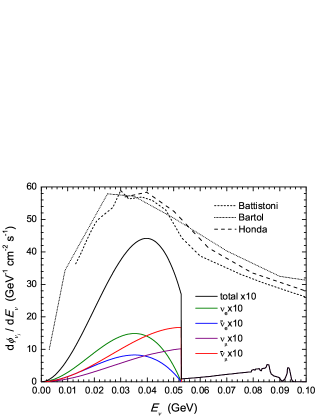
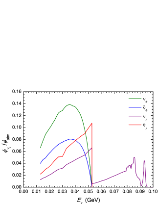
Figure 4: The differential neutrino fluxes $d\phi_{\nu_{i}}/dE_{\nu}$ (left) and the ratios of $d\phi_{\nu_{i}}/dE_{\nu}$ to the corresponding atmospheric neutrino flux from Ref. Battistoni:2005pd (right) for different flavors and $d=1000$ m. In the left panel, the total atmospheric neutrino fluxes at the Super-K site from the Bartol Gaisser:1988ar , Honda Honda:1995hz and Battistoni Battistoni:2005pd groups have also been shown.

By use of Eq. (11), we calculate the differential neutrino fluxes as shown in the left panel of Fig. 4. Here $D_{\mu^{-}}=70\%$ ($C_{\mu^{-}}=30\%$) and a Super-K detector depth $d=1000$ m have been assumed. For comparison, the total atmospheric neutrino fluxes at the Super-K site from the Bartol Gaisser:1988ar , Honda Honda:1995hz and Battistoni Battistoni:2005pd groups have also been shown. It is found that the neutrino fluxes from stopped muons are much less than the atmospheric neutrino fluxes. In the right panel of Fig. 4, we plot the ratios of $\phi_{\nu_{i}}$ to the corresponding atmospheric neutrino flux from the Battistoni group Battistoni:2005pd for different flavors. For 13 MeV $\leq E_{\nu}\leq$ 53 MeV, the $\nu_{e}$, $\bar{\nu}_{e}$, $\nu_{\mu}$ and $\bar{\nu}_{\mu}$ fluxes are averagely $10.8\%$, $6.3\%$, $3.7\%$ and $6.2\%$ of the corresponding atmospheric neutrino fluxes, respectively. It is worthwhile to stress that the above results will be increased by a factor of 1.4 if the detector depth $d<30$ m.

V Conclusions

In conclusion, we have investigated the low energy neutrinos from stopped cosmic ray muons in the Earth. The $\mu^{\pm}$ stop rates per unit volume $S_{\mu^{\pm}}(x)$ in the rock and sea water have been calculated in terms of the muon intensity $I(p_{\mu},\theta)$ at the sea level and the muon range $X(p_{\mu})$. Based on the atomic capture and nuclear capture abilities of 10 dominant elements in the upper continental crust, we estimate the $\mu^{-}$ decay and nuclear capture probabilities in the rock and sea water. Then the neutrino energy spectra $f_{\nu_{e}}$, $f_{\bar{\nu}_{e}}$, $f_{\nu_{\mu}}$ and $f_{\bar{\nu}_{\mu}}$ from a stopped muon are given. Finally, we present the low energy neutrino fluxes and give simultaneously a good approximation to calculate them. It is found that most neutrinos come from the surface distance $L<200$ km region and the near horizontal direction. For the integral fluxes $\phi_{\nu_{e}}$, $\phi_{\bar{\nu}_{\mu}}$ and $\phi_{{\nu}_{\mu}}$, the differences between the rock and water cases are very small. On the contrary, the $\phi_{\bar{\nu}_{e}}$ depends on the local rock and water distributions because of different $\mu^{-}$ decay probabilities. Note that all $\phi_{\nu_{i}}$ depend heavily on the detector depth $d$. For the Super-K detector depth $d=1000$ m, the $\nu_{e}$, $\bar{\nu}_{e}$, $\nu_{\mu}$ and $\bar{\nu}_{\mu}$ fluxes in the range of 13 MeV $\leq E_{\nu}\leq$ 53 MeV are averagely $10.8\%$, $6.3\%$, $3.7\%$ and $6.2\%$ of the corresponding atmospheric neutrino fluxes, respectively. The above results will be increased by a factor of 1.4 if the detector depth $d<30$ m. These low energy neutrinos should be considered in searches of some related topics.

- (1) Y. Fukuda et al. [Super-Kamiokande Collaboration], Phys. Rev. Lett. 81, 1562 (1998) doi:10.1103/PhysRevLett.81.1562 [hep-ex/9807003].
- (2) M. Honda, T. Kajita, K. Kasahara, S. Midorikawa and T. Sanuki, Phys. Rev. D 75, 043006 (2007) doi:10.1103/PhysRevD.75.043006 [astro-ph/0611418].
- (3) S. W. Li and J. F. Beacom, Phys. Rev. C 89, 045801 (2014) doi:10.1103/PhysRevC.89.045801 [arXiv:1402.4687 [hep-ph]].
- (4) D. F. Measday, Phys. Rept. 354, 243 (2001). doi:10.1016/S0370-1573(01)00012-6
- (5) T. K. Gaisser, T. Stanev and G. Barr, Phys. Rev. D 38, 85 (1988). doi:10.1103/PhysRevD.38.85
- (6) M. Honda, T. Kajita, K. Kasahara and S. Midorikawa, Phys. Rev. D 52, 4985 (1995) doi:10.1103/PhysRevD.52.4985 [hep-ph/9503439].
- (7) G. Battistoni, A. Ferrari, T. Montaruli and P. R. Sala, Astropart. Phys. 23, 526 (2005). doi:10.1016/j.astropartphys.2005.03.006
- (8) C. Patrignani et al. [Particle Data Group], Chin. Phys. C 40, no. 10, 100001 (2016). doi:10.1088/1674-1137/40/10/100001
- (9) S. Ando and K. Sato, New J. Phys. 6, 170 (2004) doi:10.1088/1367-2630/6/1/170 [astro-ph/0410061].
- (10) F. An et al. [JUNO Collaboration], J. Phys. G 43, no. 3, 030401 (2016) doi:10.1088/0954-3899/43/3/030401 [arXiv:1507.05613 [physics.ins-det]].
- (11) C. Rott, J. Siegal-Gaskins and J. F. Beacom, Phys. Rev. D 88, 055005 (2013) doi:10.1103/PhysRevD.88.055005 [arXiv:1208.0827 [astro-ph.HE]]; N. Bernal, J. Mart n-Albo and S. Palomares-Ruiz, JCAP 1308, 011 (2013) doi:10.1088/1475-7516/2013/08/011 [arXiv:1208.0834 [hep-ph]].
- (12) S. Palomares-Ruiz and S. Pascoli, Phys. Rev. D 77, 025025 (2008) doi:10.1103/PhysRevD.77.025025 [arXiv:0710.5420 [astro-ph]].
- (13) A. Gando et al. [KamLAND Collaboration], Astrophys. J. 745, 193 (2012) doi:10.1088/0004-637X/745/2/193 [arXiv:1105.3516 [astro-ph.HE]].
- (14) K. Ueno et al. [Super-Kamiokande Collaboration], Astropart. Phys. 36, 131 (2012) doi:10.1016/j.astropartphys.2012.05.008 [arXiv:1203.0940 [hep-ex]].
- (15) D. Reyna, hep-ph/0604145.
- (16) V. A. Naumov, hep-ph/0201310.
- (17) D. E. Groom, N. V. Mokhov and S. I. Striganov, Atom. Data Nucl. Data Tabl. 78, 183 (2001). doi:10.1006/adnd.2001.0861; http://pdg.lbl.gov/2018/AtomicNuclearProperties/
- (18) P. Coloma, P. B. Denton, M. C. Gonzalez-Garcia, M. Maltoni and T. Schwetz, JHEP 1704, 116 (2017) doi:10.1007/JHEP04(2017)116 [arXiv:1701.04828 [hep-ph]].
- (19) T. Von Egidy and F. J. Hartmann, Phys. Rev. A 26, 2355 (1982). doi:10.1103/PhysRevA.26.2355
- (20) R. L. Rudnick and S. Gao, Composition of the continental crust, pp. 1-64, (2003). In The crust (ed. R.L. Rudnick) vol. 3 Treatise on Geochemistry (eds. H.D. Holland and K.K. Turekian), Elsevier-Pergaman, Oxford; https://doi.org/10.1016/B0-08-043751-6/03016-4
- (21) T. Suzuki, D. F. Measday and J. P. Roalsvig, Phys. Rev. C 35, 2212 (1987). doi:10.1103/PhysRevC.35.2212
- (22) G. Strassner et al., Phys. Rev. C 20, 248 (1979). doi:10.1103/PhysRevC.20.248
- (23) O. L. G. Peres and A. Y. Smirnov, Phys. Rev. D 79, 113002 (2009) doi:10.1103/PhysRevD.79.113002 [arXiv:0903.5323 [hep-ph]].