Proximal Mean-field for Neural Network Quantization
Abstract
Compressing large Neural Networks (nn) by quantizing the parameters, while maintaining the performance is highly desirable due to reduced memory and time complexity. In this work, we cast nn quantization as a discrete labelling problem, and by examining relaxations, we design an efficient iterative optimization procedure that involves stochastic gradient descent followed by a projection. We prove that our simple projected gradient descent approach is, in fact, equivalent to a proximal version of the well-known mean-field method. These findings would allow the decades-old and theoretically grounded research on mrf optimization to be used to design better network quantization schemes. Our experiments on standard classification datasets (MNIST, CIFAR10/100, TinyImageNet) with convolutional and residual architectures show that our algorithm obtains fully-quantized networks with accuracies very close to the floating-point reference networks.
1 Introduction
Despite the success of deep neural networks, they are highly overparametrized, resulting in excessive computational and memory requirements. Compressing such large networks by quantizing the parameters, while maintaining the performance, is highly desirable for real-time applications, or for resource-limited devices.
In Neural Network (nn) quantization, the objective is to learn a network while restricting the parameters to take values from a small discrete set (usually binary) representing quantization levels. This can be formulated as a discrete labelling problem where each learnable parameter takes a label from the discrete set and the learning objective is to find the label configuration that minimizes the empirical loss. This is an extremely challenging discrete optimization problem because the number of label configurations grows exponentially with the number of parameters in the network and the loss function is highly non-convex.
Over the past 20 years, similar large-scale discrete labelling problems have been extensively studied under the context of Markov Random Field (mrf) optimization, and many efficient approximate algorithms have been developed [2, 6, 11, 31, 42, 43]. In this work, we take inspiration from the rich literature on mrf optimization, and design an efficient approximate algorithm based on the popular mean-field method [43] for nn quantization.
Specifically, we first formulate nn quantization as a discrete labelling problem. Then, we relax the discrete solution space to a convex polytope and introduce an algorithm to iteratively optimize the first-order Taylor approximation of the loss function over the polytope. This approach is a (stochastic) gradient descent method with an additional projection step at each iteration. For a particular choice of projection, we show that our method is equivalent to a proximal version of the well-known mean-field method. Furthermore, we prove that under certain conditions, our algorithm specializes to the popular BinaryConnect [10] algorithm.
The mrf view of nn quantization opens up many interesting research directions. In fact, our approach represents the simplest case where the nn parameters are assumed to be independent of each other. However, one can potentially model second-order or even high-order interactions among parameters and use efficient inference algorithms developed and well-studied in the mrf optimization literature. Therefore, we believe, many such algorithms can be transposed into this framework to design better network quantization schemes. Furthermore, in contrast to the existing nn quantization methods [21, 36], we quantize all the learnable parameters in the network (including biases) and our formulation can be seamlessly extended to quantization levels beyond binary.
We evaluate the merits of our algorithm on MNIST, CIFAR-10/100, and TinyImageNet classification datasets with convolutional and residual architectures. Our experiments show that the quantized networks obtained by our algorithm yield accuracies very close to the floating-point counterparts while consistently outperforming directly comparable baselines. Our code is available at https://github.com/tajanthan/pmf.
2 Neural Network Quantization
Neural Network (nn)quantization is the problem of learning neural network parameters restricted to a small discrete set representing quantization levels. This primarily relies on the hypothesis that overparametrization of nn s makes it possible to obtain a quantized network with performance comparable to the floating-point network. To this end, given a dataset , the nn quantization problem can be written as:
| (1) |
Here, is the input-output mapping composed with a standard loss function (e.g., cross-entropy loss), is the dimensional parameter vector, and with is a predefined discrete set representing quantization levels (e.g., or ). In Eq. (1), we seek a fully-quantized network where all the learnable parameters including biases are quantized. This is in contrast to the previous methods [10, 36] where some parts of the network are not quantized (e.g., biases and last layer parameters).
2.1 NN Quantization as Discrete Labelling
nn quantization (1) naturally takes the form of a discrete labelling problem where each learnable parameter takes a label from the discrete set . In particular, Eq. (1) is directly related to an mrf optimization problem [23] where the random variables correspond to the set of weights , the label set is , and the energy function is . We refer to Appendix A for a brief overview on mrf s.
An important part of an mrf is the factorization of the energy function that depends on the interactions among the random variables. While modelling a problem as an mrf, emphasis is given to the form of the energy function (e.g., submodularity) as well as the form of the interactions (cliques), because both of these aspects determine the complexity of the resulting optimization. In the case of nn s, the energy function (i.e., loss) is a composition of functions which, in general, has a variety of interactions among the random variables. For example, a parameter at the initial layer is related to parameters at the final layer via function composition. Thus, the energy function does not have an explicit factorization. In fact, optimizing Eq. (1) directly is intractable due to the following inherent problems [26, 32]:
-
1.
The solution space is discrete with exponentially many feasible points ( with in the order of millions).
-
2.
The loss function is highly non-convex and does not satisfy any regularity condition (e.g., submodularity).
-
3.
The loss function does not have an explicit factorization (corresponding to a neighbourhood structure).
This hinders the use of any off-the-shelf discrete optimization algorithm. However, to tackle the aforementioned problems, we take inspiration from the mrf optimization literature [5, 9, 43]. In particular, we first relax the discrete solution space to a convex polytope and then iteratively optimize the first-order approximation of the loss over the polytope. Our approach, as will be shown subsequently, belongs to the class of (stochastic) gradient descent methods and is applicable to any loss function. Next we describe these relaxations and the related optimization in detail.
2.2 Continuous Relaxation of the Solution Space
Recall that is a finite set of real-valued parameters. The elements of will be indexed by . An alternative representation of is by a -dimensional vector with entries . A element can be written in terms of indicator variables as , assuming that only one value of has value . Denote by the set of size of such -vectors with a single component (elements of the standard basis of ) acting as indicator vectors for the elements of . Explicitly, a vector is in set if
Similarly, the vector of all parameters can be represented using indicator variables as follows. Let be the indicator variable, where if and only if . Then, for any , we can write
| (2) |
Any represented using Eq. (2) belongs to . The vector of all parameters may be written as a matrix-vector product,
| (3) |
Here, is thought of as an matrix (each row , for is an element of ). Note that there is a one-to-one correspondence between the sets and . Substituting Eq. (3) in the nn quantization objective (1) results in the variable change from to as:
| (4) |
Even though the above variable change converts the problem from to dimensional space, the cardinalities of the sets and are the same. The binary constraint together with the non-convex loss function makes the problem NP-hard [32].
Relaxation.
By relaxing the binary constraints to , instead of we obtain the convex hull of the set . The minimization Eq. (4) may be carried out over instead of . In detail, we define
| (5) |
This is the standard -dimensional simplex embedded in and the vertices of are the points in . Similarly, the Cartesian product is the convex hull of , which are in turn the vertices of .
Simplex will be referred to as the probability simplex because an element may be thought of (formally) as a probability distribution on the finite set . A value is the probability of choosing the discrete parameter . With this probabilistic interpretation, one verifies that , the expected value of the vector of parameters , where each has independent probability distribution defined by .
Now, the relaxed optimization can be written as:
| (6) |
The minimum of this problem will generally be less than the minimum of Eq. (4). However, if , then the loss function has the same value as the original loss function . Furthermore, the relaxation of from to translates into relaxing from to the convex region . Here, and represent the minimum and maximum quantization levels, respectively.
In fact, is an overparametrized representation of , and the mapping is a many-to-one surjective mapping. In the case where (two quantization levels), the mapping is one-to-one and subjective. In addition it can be shown that any local minimum of Eq. (6) (the relaxed -space) is also a local minimum of the loss in (the relaxed -space) and vice versa (Proposition 2.1). This essentially means that the variable change from to does not alter the optimization problem and a local minimum in the -space can be obtained by optimizing in the -space.
Proposition 2.1.
Let be a function, and a point in such that . Then is a local minimum of in if and only if is a local minimum of in .
Proof.
The function is surjective continuous and affine. It follows that it is also an open map. From this the result follows easily. ∎
Finally, we would like to point out that the relaxation used while moving from to space is well studied in the mrf optimization literature and has been used to prove bounds on the quality of the solutions [9, 25]. In the case of nn quantization, in addition to the connection to mean-field (Sec. 3), we believe that this relaxation allows for exploration, which would be useful in the stochastic setting.
2.3 First-order Approximation and Optimization
Here we talk about the optimization of over , discuss how our optimization scheme allows exploration in the parameter space, and also discuss the conditions when this optimization will lead to a quantized solution in the space, which is our prime objective.
Stochastic Gradient Descent (sgd) 111The difference between sgd and gradient descent is that the gradients are approximated using a stochastic oracle in the former case. [38] is the de facto method of choice for optimizing neural networks. In this section, we interpret sgd as a proximal method, which will be useful later to show its difference to our final algorithm. In particular, sgd (or gradient descent) can be interpreted as iteratively minimizing the first-order Taylor approximation of the loss function augmented by a proximal term [34]. In our case, the objective function is the same as sgd but the feasible points are now constrained to form a convex polytope. Thus, at each iteration , the first-order objective can be written as:
| (7) |
where is the learning rate and is the stochastic (or mini-batch) gradient of with respect to evaluated at . In the unconstrained case, by setting the derivative with respect to to zero, one verifies that the above formulation leads to standard sgd updates . For constrained optimization (as in our case (2.3)), it is natural to use the stochastic version of Projected Gradient Descent (pgd) [39]. Specifically, at iteration , the projected stochastic gradient update can be written as:
| (8) |
where denotes the projection to the polytope . Even though this type of problem can be optimized using projection-free algorithms [3, 13, 27], by relying on pgd, we enable the use of any off-the-shelf first-order optimization algorithms (e.g., Adam [24]). Furthermore, for a particular choice of projection, we show that the pgd update is equivalent to a proximal version of the mean-field method.
2.3.1 Projection to the Polytope
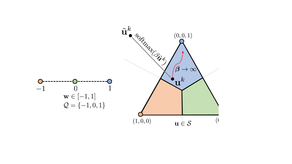
Projection to can be decomposed into independent projections to the -dimensional probability simplexes. The objective function (2.3) is also separable for each . Thus, for notational convenience, without loss of generality, we assume . Now, for a given updated parameter (where ), we discuss three approaches of projecting to the probability simplex . An illustration of these projections is shown in Fig. 1. In this section, for brevity, we also ignore the superscript .
Euclidean Projection (Sparsemax).
The standard approach of projecting to a set in the Euclidean space is via [30]. Given a scalar (usually ), amounts to finding a point in which is the closest to , namely
| (9) |
As the name suggests, this projection is likely to hit the boundary of the simplex222Unless when projected to the simplex plane is in , which is rare., resulting in sparse solutions () at every iteration. Please refer to [30] for more detail. As increases, the projected point moves towards a vertex.
Hardmax Projection.
The projection maps a given to one of the vertices of the simplex :
| (10) | ||||
| (13) |
Softmax Projection.
We now discuss the projection which projects a point to the interior of the simplex, leading to dense solutions. Given a scalar , the projection is:
| (14) | ||||
Even though approximate in the Euclidean sense, shares many desirable properties to [30] (for example, it preserves the relative order of ) and when , the projected point moves towards a vertex.
2.3.2 Exploration and Quantization using Softmax
All of the projections discussed above are valid in the sense that the projected point lies in the simplex . However, our goal is to obtain a quantized solution in the -space which is equivalent to obtaining a solution that is a vertex of the simplex . Below we provide justifications behind using with a monotonically increasing schedule for in realizing this goal, rather than either or projection.
Recall that the main reason for relaxing the feasible points to lie within the simplex is to simplify the optimization problem with the hope that optimizing this relaxation will lead to a better solution. However, in case of and projections, the effective solution space is restricted to be either the set of vertices (no relaxation) or the boundary of the simplex (much smaller subset of ). Such restrictions hinder exploration over the simplex and do not fully utilize the potential of the relaxation. In contrast, allows exploration over the entire simplex and a monotonically increasing schedule for ensures that the solution gradually approaches a vertex. This interpretation is illustrated in Fig. 1.
Entropy based view of Softmax.
In fact, can be thought of as a “noisy” projection to the set of vertices , where the noise is controlled by the hyperparameter . We now substantiate this interpretation by providing an entropy based view for the projection.
Lemma 2.1.
Let for some and . Then,
| (15) |
where is the entropy.
Proof.
This can be proved by writing the Lagrangian and setting the derivatives to zero. ∎
The projection translates into an entropy term in the objective function (15), and for small values of , it allows the iterative procedure to explore the optimization landscape. We believe, in the stochastic setting, such an explorative behaviour is crucial, especially in the early stage of training. Furthermore, our empirical results validate this hypothesis that pgd with projection is relatively easy to train and yields consistently better results compared to other pgd variants. Note that, when , the entropy term vanishes and approaches .
Note, constraining the solution space through a hyperparameter ( in our case) has been extensively studied in the optimization literature and one such example is the barrier method [7]. Moreover, even though the based pgd update yields an approximate solution to Eq. (2.3), in Sec. 3, we prove that it is theoretically equivalent to a proximal version of the mean-field method.
3 Softmax based PGD as Proximal Mean-field
Here we discuss the connection between based pgd and the well-known mean-field method [43]. Precisely, we show that the update is actually an exact fixed point update of a modified mean-field objective function. This connection bridges the gap between the mrf optimization and the nn quantization literature. We now begin with a brief review of the mean-field method and then proceed with our proof.
Mean-field Method.
A self-contained overview is provided in Appendix A, but here we review the important details. Given an energy (or loss) function and the corresponding probability distribution of the form , mean-field approximates using a fully-factorized distribution . Here, the distribution is obtained by minimizing the kl-divergence . Note that, from the probabilistic interpretation of (see Sec. 2.2), for each , the probability . Therefore, the distribution can be represented using the variables , and hence, the mean-field objective can be written as:
| (16) |
where is expectation over and is the entropy.
In fact, mean-field has been extensively studied in the mrf literature where the energy function factorizes over small subsets of variables . This leads to efficient minimization of the kl-divergence as the expectation can be computed efficiently. However, in a standard neural network, the function does not have an explicit factorization and direct minimization of the kl-divergence is not straight forward. To simplify the nn loss function one can approximate it using its first-order Taylor approximation which discards the interactions between the nn parameters altogether.
In Theorem 3.1, we show that our based pgd iteratively applies a proximal version of mean-field to the first-order approximation of . At iteration , let be the first-order Taylor approximation of . Then, since there are no interactions among parameters in , and it is linear, our proximal mean-field objective has a closed form solution, which is exactly the based pgd update.
The following theorem applies to the update of each separately, and hence the update of the corresponding parameter .
Theorem 3.1.
Let be a differentiable function defined in an open neighbourhood of the polytope , and a point in . Let be the gradient of at , and the first-order approximation of at . Let and (learning rate) be positive constants, and
| (17) |
the -based pgd update. Then,
| (18) |
Proof.
First one shows that
| (19) |
apart from constant terms (those not containing ). Then the proof follows from Lemma 2.1. ∎
The objective function Eq. (18) is essentially the same as the mean-field objective (16) for (noting up to constant terms) except for the term . This, in fact, acts as a proximal term. Note, it is the cosine similarity but subtracted from the loss to enforce proximity. Therefore, it encourages the resulting to be closer to the current point and its influence relative to the loss term is governed by the learning rate . Since gradient estimates are stochastic in our case, such a proximal term is highly desired as it encourages the updates to make a smooth transition.
Furthermore, the negative entropy term acts as a convex regularizer and when its influence becomes negligible and the update results in a binary labelling . In addition, the entropy term in Eq. (18) captures the (in)dependency between the parameters. To encode dependency, the entropy of the fully-factorized distribution can perhaps be replaced with a more complex entropy such as a tree-structured entropy, following the idea of [37]. Furthermore, in place of , a higher-order approximation can be used. Such explorations go beyond the scope of this paper.
Remark.
Note that, our update (18) can be interpreted as an entropic penalty method and it is similar in spirit to that of the mirror-descent algorithm when entropy is chosen as the mirror-map (refer Sec. 4.3 of [8]). In fact, at each iteration, both our algorithm and mirror-descent augment the gradient descent objective with a negative entropy term and optimizes over the polytope. However, compared to mirror-descent, our update additionally constitutes a proximal term and an annealing hyperparameter which enables us to gradually enforce a discrete solution. Therefore, to employ mirror-descent, one needs to understand the effects of using adaptive mirror-maps (that depend on ). Nevertheless, it is interesting to explore the potential of mirror-descent which could allow us to derive different variants of our algorithm.
Proximal Mean-Field (pmf).
The preferred embodiment of our pmf algorithm is similar to softmax based pgd. Algorithm 1 summarizes our approach. Similar to the existing methods [21], however, we introduce the auxiliary variables and perform gradient descent on them, composing the loss function with the function that maps into . In effect this solves the optimization problem:
| (20) |
In this way, optimization is carried out over the unconstrained domain rather than over the domain . In contrast to existing methods, this is not a necessity but empirically it improves the performance. Finally, since can never be , to ensure a fully-quantized network, the final quantization is performed using . Since, approaches when , the fixed points of Algorithm 1 corresponds to the fixed points of pgd with the projection. However, exploration due to allows our algorithm to converge to fixed points with better validation errors as demonstrated in the experiments.
3.1 Proximal ICM as a Special Case
For pgd, if is used instead of the projection, the resulting update is the same as a proximal version of Iterative Conditional Modes (icm) [5]. In fact, following the proof of Lemma 2.1, it can be shown that the update yields a fixed point of the following equation:
| (21) |
Notice, this is exactly the same as the icm objective augmented by the proximal term. In this case, , meaning, the feasible domain is restricted to be the vertices of the polytope . Since approaches when , this is a special case of proximal mean-field.
3.2 BinaryConnect as Proximal ICM
In this section, considering binary neural networks, i.e., , and non-stochastic setting, we show that the Proximal Iterative Conditional Modes (picm) algorithm is equivalent to the popular BinaryConnect (bc) method [10]. In these algorithms, the gradients are computed in two different spaces and therefore to alleviate any discrepancy we assume that gradients are computed using the full dataset.
Let and be the infeasible and feasible points of bc. Similarly, and be the infeasible and feasible points of our picm method, respectively. For convenience, we summarize one iteration of bc in Algorithm 2. Now, we show that the update steps in both bc and picm are equivalent.
Proposition 3.1.
Consider bc and picm with and . For an iteration , if then,
-
1.
the projections in bc: and
picm: satisfy . -
2.
let the learning rate of picm be , then the updated points after the gradient descent step in bc and picm satisfy .
Proof.
Case (1) is simply applying whereas case (2) can be proved by writing as a function of and then applying chain rule. See Appendix B. ∎
Since is a non-differentiable operation, the partial derivative is not defined. However, to allow backpropagation, we write in terms of the function, and used the straight-through-estimator [17] to allow gradient flow similar to binary connect. For details please refer to Appendix B.1.
4 Related Work
There is much work on nn quantization focusing on different aspects such as quantizing parameters [10], activations [20], loss aware quantization [18] and quantization for specialized hardware [12], to name a few. Here we give a brief summary of latest works and for a comprehensive survey we refer the reader to [15].
In this work, we consider parameter quantization, which can either be treated as a post-processing scheme [14] or incorporated into the learning process. Popular methods [10, 21] falls into the latter category and optimize the constrained problem using some form of projected stochastic gradient descent. In contrast to projection, quantization can also be enforced using a penalty term [4, 44]. Even though, our method is based on projected gradient descent, by optimizing in the -space, we provide theoretical insights based on mean-field and bridge the gap between nn quantization and mrf optimization literature.
In contrast, the variational approach can also be used for quantization, where the idea is to learn a posterior probability on the network parameters in a Bayesian framework. In this family of methods, the quantized network can be obtained either via a quantizing prior [1] or using the map estimate on the learned posterior [41]. Interestingly, the learned posterior distribution can be used to estimate the model uncertainty and in turn determine the required precision for each network parameter [29]. Note that, even in our seemingly different method, we learn a probability distribution over the parameters (see Sec. 2.2) and it would be interesting to understand the connection between Bayesian methods and our algorithm.
5 Experiments
Since neural network binarization is the most popular quantization [10, 36], we set the quantization levels to be binary, i.e., . However, our formulation is applicable to any predefined set of quantization levels given sufficient resources at training time. We would like to point out that, we quantize all learnable parameters, meaning, all quantization algorithms result in times less memory compared to the floating point counterparts.
We evaluate our Proximal Mean-Field (pmf) algorithm on MNIST, CIFAR-10, CIFAR-100 and TinyImageNet333https://tiny-imagenet.herokuapp.com/ classification datasets with convolutional and residual architectures and compare against the bc method [10] and the latest algorithm ProxQuant (pq) [4]. Note that bc and pq constitute the closest and directly comparable baselines to pmf. Furthermore, many other methods have been developed based on bc by relaxing some of the constraints, e.g., layer-wise scalars [36], and we believe, similar extensions are possible with our method as well. Our results show that the binary networks obtained by pmf yield accuracies very close to the floating point counterparts while consistently outperforming the baselines.
| Dataset | Image | # class | Train / Val. | ||
|---|---|---|---|---|---|
| MNIST | k / k | k | |||
| CIFAR-10 | k / k | k | |||
| CIFAR-100 | k / k | k | |||
| TinyImageNet | k / k | k |
| Dataset | Architecture | ref(Float) | bc [10] | pq [4] | Ours | ref- pmf | ||
| picm | pgd | pmf | ||||||
| MNIST | LeNet-300 | 98.24 | ||||||
| LeNet-5 | 99.44 | |||||||
| CIFAR-10 | VGG-16 | 90.51 | ||||||
| ResNet-18 | 92.73 | |||||||
| CIFAR-100 | VGG-16 | 61.52 | ||||||
| ResNet-18 | 71.85 | |||||||
| TinyImageNet | ResNet-18 | 51.00 | ||||||
5.1 Experiment Setup
The details of the datasets and their corresponding experiment setups are given in Table 1. In all the experiments, standard multi-class cross-entropy loss is minimized. MNIST is tested using LeNet-300 and LeNet-5, where the former consists of three fully-connected (fc) layers while the latter is composed of two convolutional and two fc layers. For CIFAR and TinyImageNet, VGG-16 [40] and ResNet-18 [16] architectures adapted for CIFAR dataset are used. In particular, for CIFAR experiments, similar to [28], the size of the fc layers of VGG-16 is set to and no dropout layers are employed. For TinyImageNet, the stride of the first convolutional layer of ResNet-18 is set to to handle the image size [19]. In all the models, batch normalization [22] (with no learnable parameters) and ReLU non-linearity are used. Except for MNIST, standard data augmentation is used (i.e., random crop and horizontal flip) and weight decay is set to unless stated otherwise.
For all the algorithms, the hyperparameters such as the optimizer and the learning rate (also its schedule) are cross-validated using the validation set444For TinyImageNet, since the ground truth labels for the test set were not available, validation set is used for both cross-validation and testing. and the chosen parameters are given in the supplementary material. For pmf and pgd with , the growth-rate in Algorithm 1 (the multiplicative factor used to increase ) is cross validated between and and chosen values for each experiment are given in supplementary. Furthermore, since the original implementation of bc do not binarize all the learnable parameters, for fair comparison, we implemented bc in our experiment setting based on the publicly available code555https://github.com/itayhubara/BinaryNet.pytorch. However, for pq we used the original code666https://github.com/allenbai01/ProxQuant, i.e., for pq, biases and last layer parameters are not binarized. All methods are trained from a random initialization and the model with the best validation accuracy is chosen for each method. Our algorithm is implemented in PyTorch [35].
5.2 Results
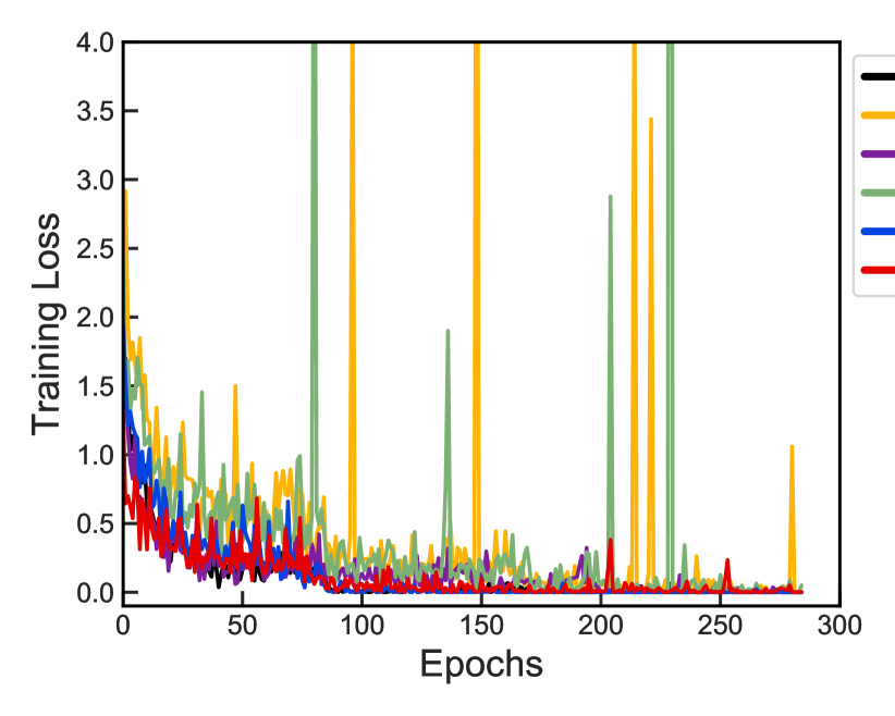
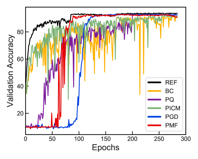
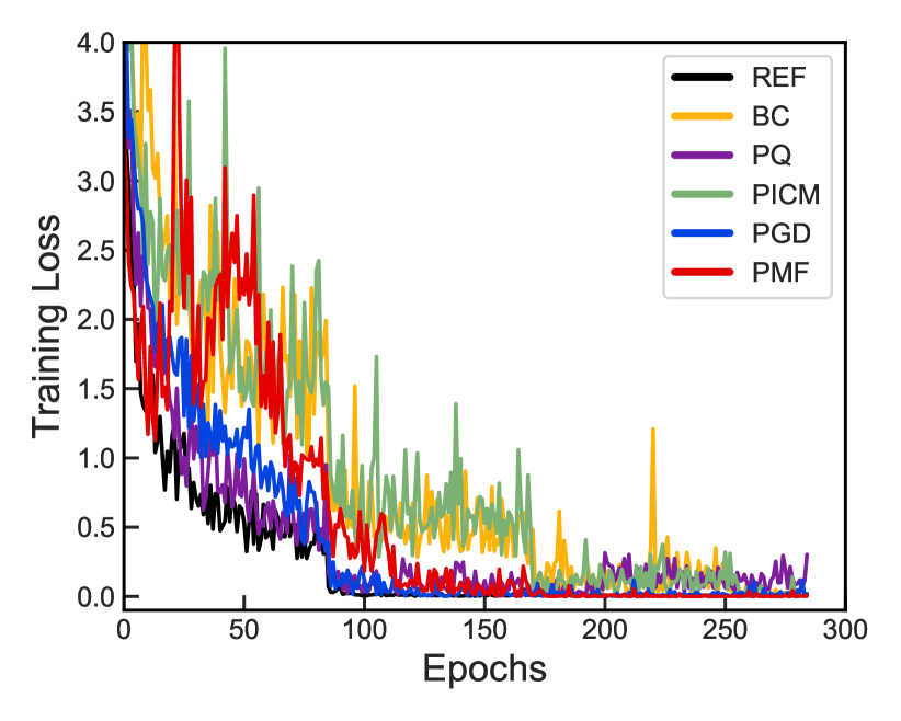
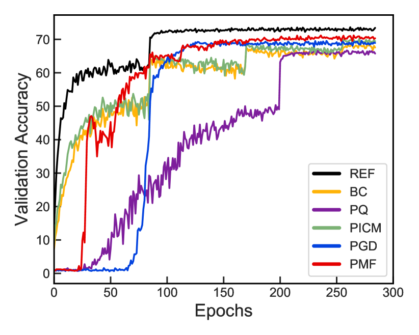
The classification accuracies (top-1) on the test set of all versions of our algorithm, namely, pmf, pgd (this is pgd with the projection), and picm, the baselines bc and pq, and the floating point Reference Network (ref) are reported in Table 2. The training curves for CIFAR-10 and CIFAR-100 with ResNet-18 are shown in Fig. 2. Note that our pmf algorithm consistently produces better results than other binarization methods and the degradation in performance to the full floating point reference network is minimal especially for small datasets. For larger datasets (e.g., CIFAR-100), binarizing ResNet-18 results in much smaller degradation compared to VGG-16.
The superior performance of pmf against bc, picm and pgd empirically validates the hypothesis that performing “noisy” projection via and annealing the noise is indeed beneficial in the stochastic setting. Furthermore, even though picm and bc are theoretically equivalent in the non-stochastic setting, picm yields slightly better accuracies in all our experiments. We conjecture that this is due to the fact that in picm, the training is performed on a larger network (i.e., in the -space).
To further consolidate our implementation of bc, we quote the accuracies reported in the original papers here. In [10], the top-1 accuracy on CIFAR-10 with a modified VGG type network is . In the same setting, even with additional layer-wise scalars, (Binary Weight Network (bwn) [36]), the corresponding accuracy is . For comprehensive results on network quantization we refer the reader to Table 5 of [15]. Note that, in all the above cases, the last layer parameters and biases in all layers were not binarized.
6 Discussion
In this work, we have formulated nn quantization as a discrete labelling problem and introduced a projected stochastic gradient descent algorithm to optimize it. By showing our approach as a proximal mean-field method, we have also provided an mrf optimization perspective to nn quantization. This connection opens up interesting research directions primarily on considering dependency between the neural network parameters to derive better network quantization schemes. Furthermore, our pmf approach learns a probability distribution over the network parameters, which is similar in spirit to Bayesian deep learning methods. Therefore, we believe, it is interesting to explore the connection between Bayesian methods and our algorithm, which can potentially drive research in both fields.
7 Acknowledgements
This work was supported by the ERC grant ERC-2012-AdG 321162-HELIOS, EPSRC grant Seebibyte EP/M013774/1, EPSRC/MURI grant EP/N019474/1 and the Australian Research Council Centre of Excellence for Robotic Vision (project number CE140100016). We would also like to acknowledge the Royal Academy of Engineering, FiveAI, National Computing Infrastructure, Australia and Nvidia (for GPU donation).
Here, we provide the proofs of propositions and theorems stated in the main paper and a self-contained overview of the mean-field method. Later in Sec. C, we give the experimental details to allow reproducibility, and more empirical analysis for our pmf algorithm.
Appendix A Mean-field Method
For completeness we briefly review the underlying theory of the mean-field method. For in-depth details, we refer the interested reader to the Chapter 5 of [43]. Furthermore, for background on Markov Random Field (mrf), we refer the reader to the Chapter 2 of [2]. In this section, we use the notations from the main paper and highlight the similarities wherever possible.
Markov Random Field.
Let be a set of random variables, where each random variable takes a label . For a given labelling , the energy associated with an mrf can be written as:
| (22) |
where is the set of subsets (cliques) of and is a positive function (factor or clique potential) that depends only on the values for . Now, the joint probability distribution over the random variables can be written as:
| (23) |
where the normalization constant is usually referred to as the partition function. From Hammersley-Clifford theorem, for the factorization given in Eq. (22), the joint probability distribution can be shown to factorize over each clique , which is essentially the Markov property. However, this Markov property is not necessary to write Eq. (23) and in turn for our formulation, but since mean-field is usually described in the context of mrf s we provide it here for completeness. The objective of mean-field is to obtain the most probable configuration, which is equivalent to minimizing the energy .
Mean-field Inference.
The basic idea behind mean-field is to approximate the intractable probability distribution with a tractable one. Specifically, mean-field obtains a fully-factorized distribution (i.e., each random variable is independent) closest to the true distribution in terms of kl-divergence. Let denote a fully-factorized distribution. Recall, the variables introduced in Sec. 2.2 represent the probability of each weight taking a label . Therefore, the distribution can be represented using the variables , where is defined as:
| (24) |
The kl-divergence between and can be written as:
| (25) | ||||
Here, denotes the entropy of the fully-factorized distribution. Specifically,
| (26) |
Furthermore, in Eq. (25), since is a constant, it can be removed from the minimization. Hence the final mean-field objective can be written as:
| (27) | ||||
where denotes the expected value of the loss over the distribution . Note that, the expected value of the loss can be written as a function of the variables . In particular,
| (28) | ||||
Now, the mean-field objective can be written as an optimization over :
| (29) |
Computing this expectation in general is intractable as the sum is over an exponential number of elements ( elements, where is usually in the order millions for an image or a neural network). However, for an mrf, the energy function can be factorized easily as in Eq. (22) (e.g., unary and pairwise terms) and can be computed fairly easily as the distribution is also fully-factorized.
In mean-field, the above objective (29) is minimized iteratively using a fixed point update. This update is derived by writing the Lagrangian and setting the derivatives with respect to to zero. At iteration , the mean-field update for each can be written as:
| (30) |
Here, denotes the gradient of with respect to evaluated at . This update is repeated until convergence. Once the distribution is obtained, finding the most probable configuration is straight forward, since is a product of independent distributions over each random variable . Note that, as most probable configuration is exactly the minimum label configuration, the mean-field method iteratively minimizes the actual energy function .
Appendix B BinaryConnect as Proximal ICM
Proposition B.1.
Consider bc and picm with and . For an iteration , if then,
-
1.
the projections in bc: and
picm: satisfy . -
2.
let the learning rate of picm be , then the updated points after the gradient descent step in bc and picm satisfy .
Proof.
-
1.
In the binary case (), for each , the projection can be written as:
(32) Now, multiplying both sides by , and substituting ,
(34) Hence, .
-
2.
Since from case (1) above, by chain rule the gradients and satisfy,
(35) Similarly, from case (1) above, for each ,
(36) Here, the partial derivatives are evaluated at but omitted for notational clarity. Moreover, is a -dimensional column vector, is a scalar, and is a matrix. Since, (similar to Eq. (35)),
(37) Now, consider the for each ,
(38) Now, consider the gradient descent step for , with ,
(39) Hence, the proof is complete.
∎
Note that, in the implementation of bc, the auxiliary variables are clipped between as it does not affect the function. In the -space, this clipping operation would translate into a projection to the polytope , meaning implies , where and are related according to . Even in this case, Proposition B.1 holds, as the assumption is still satisfied.
B.1 Approximate Gradients through Hardmax
In previous works [10, 36], to allow back propagation through the function, the straight-through-estimator [17] is used. Precisely, the partial derivative with respect to the function is defined as:
| (40) |
To make use of this, we intend to write the projection function in terms of the function. To this end, from Eq. (1), for each ,
| (43) | ||||
| (44) |
Hence, the projection for each can be written as:
| (45) | ||||
| (46) |
Now, using Eq. (40), we can write:
| (47) |
where .
Appendix C Experimental Details
To enable reproducibility, we first give the hyperparameter settings used to obtain the results reported in the main paper in Table 4.
| Dataset | Architecture | pmf wo | pmf |
|---|---|---|---|
| MNIST | LeNet-300 | 98.24 | |
| LeNet-5 | 99.44 | ||
| CIFAR-10 | VGG-16 | 90.51 | |
| ResNet-18 | 92.73 |
C.1 Proximal Mean-field Analysis
To analyse the effect of storing the auxiliary variables in Algorithm 1, we evaluate pmf with and without storing , meaning the variables are updated directly. The results are reported in Table 3. Storing the auxiliary variables and updating them is in fact improves the overall performance. However, even without storing , pmf obtains reasonable performance, indicating the usefulness of our continuous relaxation. Note that, if the auxiliary variables are not stored in bc, it is impossible to train the network as the quantization error in the gradients are catastrophic and single gradient step is not sufficient to move from one discrete point to the next.
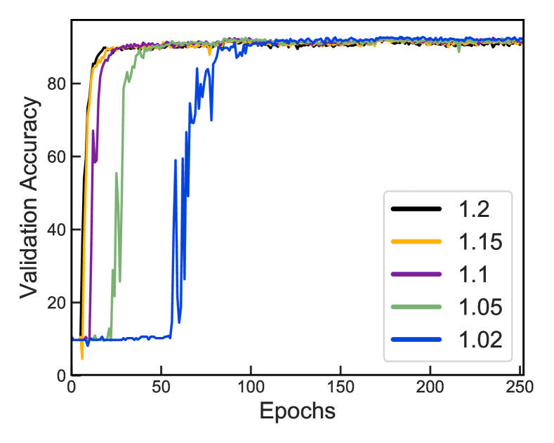
C.2 Effect of Annealing Hyperparameter
In Algorithm 1, the annealing hyperparameter is gradually increased by a multiplicative scheme. Precisely, is updated according to for some . Such a multiplicative continuation is a simple scheme suggested in Chapter 17 of [33] for penalty methods. To examine the sensitivity of the continuation parameter , we report the behaviour of pmf on CIFAR-10 with ResNet-18 for various values of in Fig. 3.
C.3 Multi-bit Quantization
To test the performance of pmf for quantization levels beyond binary, we ran pmf for -bit quantization with on CIFAR-10 with the same hyperparameters as in the binary case and the results are, ResNet-18: % and VGG-16: %, respectively. We believe, the improvements over binary (% and %) even without hyperparameter tuning shows the merits of pmf for NN quantization. Note, similar to existing methods [4], we can also obtain different quantization levels for each weight , which would further improve the performance.
| Hyperparameter | MNIST with LeNet-300/5 | TinyImageNet with ResNet-18 | ||||||||
|---|---|---|---|---|---|---|---|---|---|---|
| ref | bc/picm | pq | pgd | pmf | ref | bc/picm | pq | pgd | pmf | |
| learning_rate | 0.001 | 0.001 | 0.01 | 0.001 | 0.001 | 0.1 | 0.0001 | 0.01 | 0.1 | 0.001 |
| lr_decay | step | step | - | step | step | step | step | step | step | step |
| lr_interval | 7k | 7k | - | 7k | 7k | 60k | 30k | 30k | 30k | 30k |
| lr_scale | 0.2 | 0.2 | - | 0.2 | 0.2 | 0.2 | 0.2 | 0.2 | 0.2 | 0.2 |
| momentum | - | - | - | - | - | 0.9 | - | - | 0.95 | - |
| optimizer | Adam | Adam | Adam | Adam | Adam | sgd | Adam | Adam | sgd | Adam |
| weight_decay | 0 | 0 | 0 | 0 | 0 | 0.0001 | 0.0001 | 0.0001 | 0.0001 | 0.0001 |
| (ours) or reg_rate (pq) | - | - | 0.001 | 1.2 | 1.2 | - | - | 0.0001 | 1.01 | 1.02 |
| CIFAR-10 with VGG-16 | CIFAR-10 with ResNet-18 | |||||||||
| ref | bc/picm | pq | pgd | pmf | ref | bc/picm | pq | pgd | pmf | |
| learning_rate | 0.1 | 0.0001 | 0.01 | 0.0001 | 0.001 | 0.1 | 0.0001 | 0.01 | 0.1 | 0.001 |
| lr_decay | step | step | - | step | step | step | step | - | step | step |
| lr_interval | 30k | 30k | - | 30k | 30k | 30k | 30k | - | 30k | 30k |
| lr_scale | 0.2 | 0.2 | - | 0.2 | 0.2 | 0.2 | 0.2 | - | 0.2 | 0.2 |
| momentum | 0.9 | - | - | - | - | 0.9 | - | - | 0.9 | - |
| optimizer | sgd | Adam | Adam | Adam | Adam | sgd | Adam | Adam | sgd | Adam |
| weight_decay | 0.0005 | 0.0001 | 0.0001 | 0.0001 | 0.0001 | 0.0005 | 0.0001 | 0.0001 | 0.0001 | 0.0001 |
| (ours) or reg_rate (pq) | - | - | 0.0001 | 1.05 | 1.05 | - | - | 0.0001 | 1.01 | 1.02 |
| CIFAR-100 with VGG-16 | CIFAR-100 with ResNet-18 | |||||||||
| ref | bc/picm | pq | pgd | pmf | ref | bc/picm | pq | pgd | pmf | |
| learning_rate | 0.1 | 0.01 | 0.01 | 0.0001 | 0.0001 | 0.1 | 0.0001 | 0.01 | 0.1 | 0.001 |
| lr_decay | step | multi-step | - | step | step | step | step | step | step | multi-step |
| lr_interval | 30k | 20k - 80k, | - | 30k | 30k | 30k | 30k | 30k | 30k | 30k - 80k, |
| every 10k | every 10k | |||||||||
| lr_scale | 0.2 | 0.5 | - | 0.2 | 0.2 | 0.1 | 0.2 | 0.2 | 0.2 | 0.5 |
| momentum | 0.9 | 0.9 | - | - | - | 0.9 | - | - | 0.95 | 0.95 |
| optimizer | sgd | sgd | Adam | Adam | Adam | sgd | Adam | Adam | sgd | sgd |
| weight_decay | 0.0005 | 0.0001 | 0.0001 | 0.0001 | 0.0001 | 0.0005 | 0.0001 | 0.0001 | 0.0001 | 0.0001 |
| (ours) or reg_rate (pq) | - | - | 0.0001 | 1.01 | 1.05 | - | - | 0.0001 | 1.01 | 1.05 |
References
- [1] J. Achterhold, J. M. Kohler, A. Schmeink, and T. Genewein. Variational network quantization. ICLR, 2018.
- [2] Thalaiyasingam Ajanthan. Optimization of Markov random fields in computer vision. PhD thesis, Australian National University, 2017.
- [3] Thalaiyasingam Ajanthan, Alban Desmaison, Rudy Bunel, Mathieu Salzmann, Philip H S Torr, and M Pawan Kumar. Efficient linear programming for dense CRFs. CVPR, 2017.
- [4] Yu Bai, Yu-Xiang Wang, and Edo Liberty. Proxquant: Quantized neural networks via proximal operators. ICLR, 2019.
- [5] Julian Besag. On the statistical analysis of dirty pictures. Journal of the Royal Statistical Society., 1986.
- [6] Andrew Blake, Pushmeet Kohli, and Carsten Rother. Markov random fields for vision and image processing. Mit Press, 2011.
- [7] Stephen Boyd and Lieven Vandenberghe. Convex optimization. Cambridge university press, 2009.
- [8] Sébastien Bubeck. Convex optimization: Algorithms and complexity. Foundations and Trends® in Machine Learning, 2015.
- [9] Chandra Chekuri, Sanjeev Khanna, Joseph Naor, and Leonid Zosin. A linear programming formulation and approximation algorithms for the metric labeling problem. SIAM Journal on Discrete Mathematics, 2004.
- [10] Matthieu Courbariaux, Yoshua Bengio, and Jean-Pierre David. Binaryconnect: Training deep neural networks with binary weights during propagations. NIPS, 2015.
- [11] P. K. Dokania and P. K. Mudigonda. Parsimonious labeling. ICCV, 2015.
- [12] S. K. Esser, R. Appuswamy, P. A. Merolla, J. V. Arthur, and D. S. Modha. Backpropagation for energy-efficient neuromorphic computing. NIPS, 2015.
- [13] Marguerite Frank and Philip Wolfe. An algorithm for quadratic programming. Naval research logistics quarterly, 1956.
- [14] Y. Gong, L. Liu, and L. Bourdev. Compressing deep convolutional networks using vector quantization. arXiv preprint arXiv:1412.6115, 2014.
- [15] Yunhui Guo. A survey on methods and theories of quantized neural networks. arXiv preprint arXiv:1808.04752, 2018.
- [16] Kaiming He, Xiangyu Zhang, Shaoqing Ren, and Jian Sun. Deep residual learning for image recognition. CVPR, 2016.
- [17] Geoffrey Hinton. Neural networks for machine learning. Coursera, video lectures, 2012.
- [18] Lu Hou, Quanming Yao, and James T Kwok. Loss-aware binarization of deep networks. ICLR, 2017.
- [19] Gao Huang, Yixuan Li, Geoff Pleiss, Zhuang Liu, John E Hopcroft, and Kilian Q Weinberger. Snapshot ensembles: Train 1, get m for free. ICLR, 2017.
- [20] Itay Hubara, Matthieu Courbariaux, Daniel Soudry, Ran El-Yaniv, and Yoshua Bengio. Binarized neural networks. NIPS, 2016.
- [21] Itay Hubara, Matthieu Courbariaux, Daniel Soudry, Ran El-Yaniv, and Yoshua Bengio. Quantized neural networks: Training neural networks with low precision weights and activations. JMLR, 2017.
- [22] Sergey Ioffe and Christian Szegedy. Batch normalization: Accelerating deep network training by reducing internal covariate shift. ICML, 2015.
- [23] R. Kindermann and J. L. Snell. Markov Random Fields and Their Applications. American Mathematical Society, 1980.
- [24] Diederik P Kingma and Jimmy Ba. Adam: A method for stochastic optimization. ICLR, 2015.
- [25] Jon Kleinberg and Eva Tardos. Approximation algorithms for classification problems with pairwise relationships: metric labeling and Markov random fields. Journal of the ACM, 2002.
- [26] Vladimir Kolmogorov and Ramin Zabin. What energy functions can be minimized via graph cuts? PAMI, 2004.
- [27] Simon Lacoste-Julien, Martin Jaggi, Mark Schmidt, and Patrick Pletscher. Block-coordinate Frank-Wolfe optimization for structural SVMs. ICML, 2012.
- [28] Namhoon Lee, Thalaiyasingam Ajanthan, and Philip H S Torr. SNIP: Single-shot network pruning based on connection sensitivity. ICLR, 2019.
- [29] C. Louizos, K. Ullrich, and M. Welling. Bayesian compression for deep learning. NIPS, 2017.
- [30] Andre Martins and Ramon Astudillo. From softmax to sparsemax: A sparse model of attention and multi-label classification. ICML, 2016.
- [31] Pawan Kumar Mudigonda. Combinatorial and convex optimization for probabilistic models in computer vision. PhD thesis, Oxford Brookes University, 2008.
- [32] George L Nemhauser and Laurence A Wolsey. Integer programming and combinatorial optimization. Springer, 1988.
- [33] Jorge Nocedal and Stephen Wright. Numerical optimization. Springer, 2006.
- [34] Neal Parikh and Stephen P Boyd. Proximal algorithms. Foundations and Trends in Optimization, 2014.
- [35] Adam Paszke, Sam Gross, Soumith Chintala, Gregory Chanan, Edward Yang, Zachary DeVito, Zeming Lin, Alban Desmaison, Luca Antiga, and Adam Lerer. Automatic differentiation in PyTorch. 2017.
- [36] Mohammad Rastegari, Vicente Ordonez, Joseph Redmon, and Ali Farhadi. Xnor-net: Imagenet classification using binary convolutional neural networks. ECCV, 2016.
- [37] Pradeep Ravikumar, Alekh Agarwal, and Martin J Wainwright. Message-passing for graph-structured linear programs: proximal projections, convergence and rounding schemes. ICML, 2008.
- [38] Herbert Robbins and Sutton Monro. A stochastic approximation method. Annals of Mathematical Statistics, 1951.
- [39] Lorenzo Rosasco, Silvia Villa, and Bang Công Vũ. Convergence of stochastic proximal gradient algorithm. arXiv preprint arXiv:1403.5074, 2014.
- [40] Karen Simonyan and Andrew Zisserman. Very deep convolutional networks for large-scale image recognition. ICLR, 2015.
- [41] D. Soudry, I. Hubara, and R. Meir. Expectation backpropagation: Parameter-free training of multilayer neural networks with continuous or discrete weights. NIPS, 2018.
- [42] Olga Veksler. Efficient graph-based energy minimization methods in computer vision. PhD thesis, Cornell University New York, USA, 1999.
- [43] Martin J Wainwright, Michael I Jordan, et al. Graphical models, exponential families, and variational inference. Foundations and Trends® in Machine Learning, 2008.
- [44] Penghang Yin, Shuai Zhang, Jiancheng Lyu, Stanley Osher, Yingyong Qi, and Jack Xin. Binaryrelax: A relaxation approach for training deep neural networks with quantized weights. SIIMS, 2018.