Stripe phase of two-dimensional core-softened systems: structure recognition

Abstract

In the present paper we discuss a so called stripe phase of two-dimensional systems which was observed in computer simulation of core-softened system and in some experiments with colloidal films. We show that the stripe phase is indeed an oblique crystal and find out its unit vectors, i.e. we give a full description of the structure of this crystalline phase.

Investigation of two-dimensional (2d) systems is of great interest for many fundamental and technological issues. They demonstrate many unusual features which make them especially interesting. The most striking example is the melting of 2d crystals. While in three dimensions (3d) melting occurs as the first order phase transition only, three most plausible mechanisms of melting of 2d crystals are known at the moment ufn . At the same time until recently it was supposed that 2d systems do not demonstrate great variety of ordered structures. Only triangular crystal was observed in experimental studies. However, in the last decade many experimental investigations demonstrated that 2d and quasi-2d systems do demonstrate other crystalline structures too. Formation of square ice when water is confined between two graphite planes was reported in Ref. geim . The square phase of one atom thick layer of iron on graphite was also observed in Ref. iron . Even more complex phases were observed in 2d colloidal systems dobnikar . However, until now experimental observations of ordered 2d structures except triangular lattice are rather rare.

At the same time complex 2d structures are widely discussed in frames of computer simulation studies. There are numerous publications which demonstrate existence of different crystalline and quasicrystalline structures in 2d systems (see, for instance, hzmiller ; hzch ; hzwe ; we1 ; we2 ; we3 ; we4 ; we5 ; trusket2 ; trusket3 ; trusket4 ; qc1 ; qc2 ; qc3 and references therein). A model core-softened system (smooth repulsive shoulder SRS) was proposed in Ref. we-init . The potential of this system is defined as

$$U(r)/\varepsilon=\left(\frac{d}{r}\right)^{n}+0.5\left(1-tanh(k(r-\sigma))\right),$$ (1)

where $n=14$, $k=10$ and the parameter $\sigma$ determines the width of the repulsive shoulder of the potential. It was shown that the phase diagram of three dimensional SRS system is very complex, with numerous crystalline phases, maxima on the melting line, etc. The behavior of the same system in 2d was investigated in Refs. we1 ; we2 ; we3 ; we4 ; we5 . According to these publications, while at $\sigma=1.15$ the system demonstrates only triangular crystalline phase, at $\sigma=1.35$ square crystal and dodecagonal quasicrystal are found.

The SRS system was generalized in Ref. we-attract by adding an attractive well to the potential (SRS - attractive well system - SRS-AW):

$$U(r)/\varepsilon=\left(\frac{d}{r}\right)^{n}+\sum_{i=1}^{2}\left(1-tanh(k_{i}(r-\sigma_{i}))\right).$$ (2)

Phase diagrams and anomalous behavior of 3d SRS-AW system with different parameters of the potential were investigated we-attract ; we-attract1 ; we-attract2 ; we-attract3 . Later on in a number of publications it was realized that varying the parameters of SRS-AW system different complex crystalline structures both in 2d and 3d can be obtained. In Ref. str2d3d a method of finding a potential which stabilizes a particular crystalline structure was proposed and potentials which stabilize square and honeycomb lattices were obtained. This method was used to find parametrization of SRS-AW potential to stabilize different 2d and 3d structures including Kagome lattice, snub-square tiling, honeycomb lattice in the case of 2d systems and cubic and diamond structures for the 3d ones trusket1 ; trusket2 ; trusket3 ; trusket4 .

A particular structure which was found in some 2d systems is the so called stripe phase. Stripe phases are known in many different system including magnetic films, Langmuir monolayers, polymer films, etc. In the case of atomic systems the formation of stripe phase is usually attributed to the competition of short-range attraction between the particles and long-range dipole-dipole interaction. Basing on this assumption a model was proposed in Ref. camp where the interaction potential consists of Lennard-Jones term and long range dipole-dipole term. Rather small system (500 particles) was studied in this paper. A larger system of 2000 particles was simulated in addition to check for the finite size effects. It was discovered that at some density-temperature points systems of 500 particles form a lamellar phase. However, in case of larger system the lamellar phase was not formed (see Fig. 12 of Ref. camp ). Instead of this the stripe phase was observed which differs from the lamellar one in the sense that the threads of the particles becomes curved rather then linear. Because of this it was concluded that the lamellar phase was artificially stabilized by the periodic boundary conditions and the stripe phase is the stable one. Moreover, it was stated that the stripe phase is a indeed a cluster fluid. These results were confirmed in the subsequent publication of the same author camp1 .

Formation of the stripe phase was discovered in the simplest core-softened system - repulsive step potential malpel ; norizoe ; norizoe1 ; dijkstra . The stripe phase was observed for several different values of the width of the step. In particular, in Ref. malpel the authors reported a peak of the heat capacity which appears in the system upon heating. Fig. 3 of Ref. malpel reports snapshots of the system above the peak of the heat capacity and below it. In Fig. 3 of Ref. malpel one can see snapshots of the system below and above the peak of the heat capacity. The structure below the peak corresponds to lamellar phase in terms of Ref. camp while the structure above the peak looks like the stripe phase in camp . In this respect the results of these publications appear to be qualitatively different: while in camp the change from the structure with linear threads of the particles (lamellar phase) to the structure with curved threads (stripe phase) is related to the finite size effects, in malpel these structures are separated by the phase transition, i.e. they are two different phases.

Importantly, most of the authors reported the existence of the stripe phase but did not try to describe its structure. The only work where an attempt to describe the structure of the stripe phase is Ref. dijkstra (see eqs. (7) and (8)).

In Ref. genetic the ground states of the repulsive step potential were investigated. The structures were obtained by genetic algorithms optimization. The authors did not find anything like stripe phase. However, the values of the step width reported in genetic are 1.5, 3.0, 7.0 and 10.0. In Ref. norizoe it was argued that at these values of the width no stripe phase is found.

In Ref. dobnikar an experimental study of colloidal particles in magnetic field was performed. The sequence of phases which the authors observed was very similar to the one obtained in the computational work camp . In particular, it was found that the experimental system does demonstrate the stripe phase.

In the present paper we perform a computational study of stripe phase in a core-softened system. We carry out the analysis of its structure. We find that the stripe phase is in fact a crystalline structure and find its unit cell.

A	0.01978
n	5.49978
$\lambda_{1}$	-0.06066
$k_{1}$	2.53278
$d_{1}$	1.94071
$\lambda_{2}$	1.06271
$k_{2}$	1.73321
$d_{2}$	1.04372
$r_{c}$	3.0
$P$	0.007379
$Q$	0.04986
$R$	-0.085054

Table 1: The parameters of the potential 3 used in the present study.

Following Ref. trusket4 let us rewrite the potential 2 in the following form:

$$U(r)/\varepsilon=A\left(\frac{\sigma}{r}\right)^{n}+\sum_{i=1}^{2}\lambda_{i}\left(1-tanh(k_{i}(r/\sigma-d_{i}))\right)+U_{shift}$$ (3)

where $U_{shift}=Pr^{2}+Qr+R$ is used to make both the potential and its first and second derivative continuous at the cut-off distance $r_{c}$. We use the parameterizations of the potential which stabilizes the Kagome lattice trusket4 . The parameters of the potential are taken from Ref. trusket4 . For the convenience of the reader they are given in Table I. We find that at the densities below the ones where the Kagome lattice is stable the system demonstrates the stripe phase. The full phase diagram of this system will be a topic of a subsequent publication.

In the remainder of this paper we use the dimensionless quantities, which in $2D$ have the form: $\tilde{{\bf r}}\equiv{\bf r}/\sigma$, $\tilde{P}\equiv P\sigma^{2}/\varepsilon,$ $\tilde{V}\equiv V/N\sigma^{2}\equiv 1/\tilde{\rho},\tilde{T}\equiv k_{B}T/\varepsilon$, $\tilde{t}=\sigma(m/\varepsilon)^{1/2}$, where $m=1$ is the mass of the particles which is used as a unit of mass., etc. In the rest of the article the tildes will be omitted.

Initially we simulate a system of 5000 particles in a rectangular box with periodic boundary conditions by means of molecular dynamics method in order to find the region of stability of the stripe phase. The system is simulated for $5\cdot 10^{6}$ steps. The time step is set to $dt=0.001$. The first $3\cdot 10^{6}$ are used for equilibration while during the last $2\cdot 10^{6}$ we collect the data. We calculate the equations of state and the radial distribution functions of the system. The system is simulated in NVT ensemble (constant number of particles N, volume V and temperature T). Nose-Hoover thermostat with time parameter $\tau=0.01$ is used.

Fig. 1 shows an instantaneous configuration of the system at the density $\rho=0.9$ and temperature $T=0.01$. One can see that this system is in lamellar phase in terminology of Camp camp and stripe phase in terminology of Malescio and Pelicane malpel . Camp observed such a phase in a small system of 500 particles. In a larger system he found that the lines of particles deviate from the linear shape and concluded that lamellar phase is a consequence of the periodic boundary conditions (see Fig. 12 in Ref. camp ). We also observe such phase. However, simulating the system for longer time we find that the threads become strainght and the system comes into lamellar phase. Because of this we suppose that the configuration shown in Fig. 12b of Ref. camp is not completely equilibrated one.

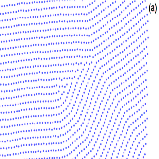
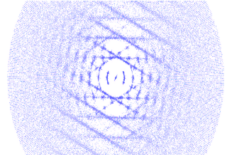
Figure 1: (a) A snapshot of the system at $\rho=0.9$ and $T=0.005$; (b) radial distribution function of the system at the same parameters. The inset enlarger the region of small $r$; (c) the diffraction pattern at the same parameters.

In Ref. malpel it was assumed that such a structure demonstrates long-range orientational ordering, but not translational one. Fig. 1 (b) shows the rdf of this system at the same point $\rho=0.9$ and $T=0.005$. One can see that it demonstrated clear long-range order. We also calculate the diffraction pattern of the system. The diffraction pattern is calculated as $S(\bf{k})=<\frac{1}{N}\left(\sum_{i}^{N}cos(\bf{kr}_{i})\right)^{2}+\left(\sum_{i}^{N}sin(\bf{kr}_{i})\right)^{2}>$. The results are shown in Fig. 1 (c)) and they demonstrate that the system is in crystalline phase. Therefore, in order to describe this structure one needs to find the parameters of the unit cell.

Let us draw the structure by bonds rather then points (Fig.  2). We connect two particles by a bond if they are closer then some distance $r_{b}$. The parameter $r_{b}$ is selected in such a way that the system demonstrates a clear pattern: below $r_{b}$ many particles are not connected or connected to a single particle only while above it the particles are connected to many other particles. Here $r_{b}=1.6$ One can see that the main motif is a triangle. The sides of the triangle can be taken as the locations of the first three maxima of the rdf. From Fig.  1 we obtain $r_{1}=0.78227$ (side AB), $r_{2}=1.46189$ (side BC) and $r_{3}=1.56808$ (side AC). From basic geometry we obtain $cos(\gamma)=0.38$. One can choose the vectors AB and AC (Fig.  2 (b)) as the basic vectors. Their coordinates are $\textbf{a}=\textbf{AB}=(a,0)$, where $a=AB=0.78227$ and $\textbf{b}=\textbf{AC}=(bcos\gamma,bsin\gamma$), where $b=AC=1.56808$. Below we will call the structure with these basic vectors as oblique phase.

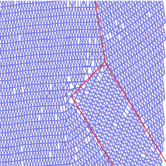
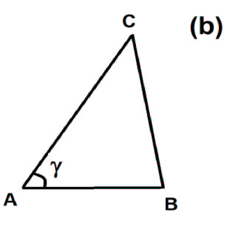
Figure 2: (a) A snapshot of the system at $\rho=0.9$ and $T=0.005$ drawn by bonds. The lines show the grain boundaries; (b) a cartoon of the base triangle of the structure. AB=0.78227, AC=1.56808, BC=1.46189.

We construct the lattice with basis vectors $\bf{a}$ and $\bf{b}$. It is a rhomboid structure with the tilt angle $\gamma$. In the present study we use a system which contains 20000 particles. We simulate the system at constant pressure $P=P_{xx}=P_{yy}$. The diagonal component of the pressure $P_{xy}$ was set to zero, since in equilibrium there should not be any tangential stresses in the system. The sides and the tilt angle could vary independently in the course of simulation. Parinello-Rahman thermostat is used. Longer simulations of $5\cdot 10^{7}$ steps are performed in order to ensure that the structure is stable.

From molecular dynamics simulation of the oblique phase we observe that the oblique structure is stable. The limits of stability of this structure at $T=0.01$ are from $P_{min}=2.3$ and up to $P_{max}=5.0$ . At larger pressures the system transforms into Kagome lattice, while at smaller ones into the phase of dimers. The full phase diagram of this system will be published in the subsequent paper. The average tilt angle at different pressures varies from $cos(\gamma)=0.407$ up to $cos(\gamma)=0.422$.

Fig.  3 gives a comparison of equations of states obtained in rectangular and tilted boxes. One can see that these equations of state are in perfect agreement which means that the phases obtained in both types of boxes are the same.

Fig.  4 (a) shows a snapshot of the system simulated in tilted box at $T=0.01$ and $P=2.4$. This point belongs to the stripe phase in terminology of Refs. malpel . One can see that the system preserves the crystalline order of the oblique phase. Figs.  4 (b) and (c) compare the rdfs of the system at two points of stability of the stripe phase computed in rectangular and tilted boxes. The rdfs of the rectangular and tilted system are in perfect agreement which confirms that the stripe phase is a polycrystalline sample of the oblique phase.

We simulate the tilted system at constant density $\rho=0.9$ and temperature from $T_{min}=0.005$ up to $T=0.05$ and at constant pressure $P=3.0$ and temperature from $T=0.002$ up to $T=0.005$. The tilt angle is set to $cos(\gamma)=0.415$. Fig.  5 shows the pressure, isochoric heat capacity and diffusion coefficient at the isochor $\rho=0.9$. The heat capacity is obtained by numerical differentiation of the internal energy. One can see that there is a bend in the pressure and diffusion coefficients at $T=0.0032$. The heat capacity demonstrates a peak at the same temperature. Similar peak was observed by Malescio and Pelicane in Ref. malpel . At the same time we see that the diffusion coefficient at the temperatures above the heat capacity peak has liquid-like magnitudes.

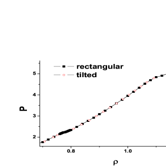
Figure 3: Comparison of equations of states obtained by simulations in rectangular and tilted boxes at $T=0.01$.

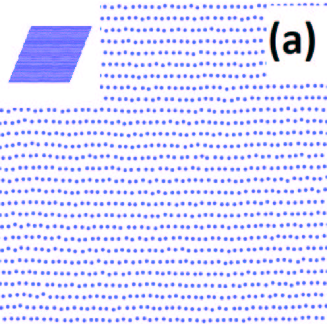
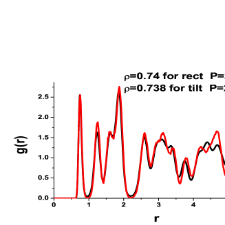
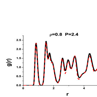
Figure 4: (a) Snapshot of the system simulated in the tilted box at $T=0.01$ and $P=2.4$. In the left upper corner we show the whole box to demonstrate that it is tilted. The snapshot itself enlarges a part of the system to see that particles. (b) Comparison of rdfs of rectangular and tilted systems at $\rho=0.74$, $T=0.01$; (b) The same at $\rho=0.8$, $T=0.01$.

Figure 5: (a) Pressure of the oblique system along the isochor $\rho=0.9$; (b) isochoric heat capacity along the same isochor. The inset shows the internal energy along the same isochor. (c) Diffusion coefficient of the same system.

Fig.  6 shows the rdf and diffraction pattern of the system at $\rho=0.9$ and $T=0.04$, which is above the peak of the heat capacity. Although rdf demonstrates several peaks it corresponds to liquid phase. The same conclusion can be made from the diffraction pattern. Combining it with large magnitude of the diffusion coefficient we conclude that this phase is liquid.

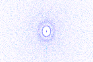
Figure 6: (a) Radial distribution function at $\rho=0.9$ and $T=0.04$. (b) Diffraction pattern at the same point.

Similar observations are made along the isobar $P=3.0$. The corresponding plots are given in Supplementary materials.

Fig. 7 shows the equation of state and the isobaric heat capacity. The heat capacity is obtained by numerical differentiation of the enthalpy. One can see qualitatively the same picture. The temperature dependence of density demonstrates a bend at $T=0.032$ and the heat capacity has a peak at the same temperature. The results on the heat capacities confirm that there is a phase transition in the system which is in agreement with Ref. malpel .

Figure 7: (a) Equation of state along the isobar $P=3.0$ (b) isobaric heat capacity along the same isobar. The inset shows the enthalpy along the same isobar.

In conclusion, we find that stripe phase which is widely discussed in the literature is indeed a crystalline phase made of tilted triangles (oblique phase). The oblique phase was already observed as a ground state structure of some core-softened systems trusket2 ; genetic , however it was not recognized that this phase is the same with stripe phase which was reported by several authors in core-softened systems at finite temperature. We find the unit vectors of the oblique phase. When the temperature is risen it transforms into correlated liquid. From the snapshots of this liquid one can see that it contains some small stripes. However, no long range order is observed in this liquid phase.

This work was carried out using computing resources of the federal collective usage center ”Complex for simulation and data processing for mega-science facilities” at NRC ”Kurchatov Institute”, http://ckp.nrcki.ru, and supercomputers at Joint Supercomputer Center of the Russian Academy of Sciences (JSCC RAS). The work was supported by the Russian Science Foundation (Grant No 14-22-00093).

References

- (1) V. N. Ryzhov, E. E. Tareyeva, Yu. D. Fomin, and E. N. Tsiok, Phys. Usp. 60 857 885 (2017).
- (2) G. Algara-Siller, O. Lehtinen, F. C. Wang, R. R. Nair, U. Kaiser, H. A.Wu, A. K. Geim and I. V. Grigorieva, Nature 519, 443 (2015).
- (3) Jiong Zhao et al., Science 343, 1228 (2014).
- (4) N. Osterman, D. ,1 I. Poberaj, J. Dobnikar, and P. Ziherl, Phys. Rev. Lett. 99, 248301 (2007).
- (5) W.L. Miller and A. Cacciuto, Soft Matter 7, 7552 (2011).
- (6) M. Zu, P. Tan, and N. Xu, Nat. Comm. 8, 2089 (2017).
- (7) Yu. D. Fomin, E. A. Gaiduk, E. N. Tsiok, and V. N. Ryzhov, Mol. Phys. 116 (21-22), 3258-3270 (2018).
- (8) D.E. Dudalov, Yu.D. Fomin, E.N. Tsiok, and V.N. Ryzhov, Journal of Physics: Conference Series 510 (2014) 012016.
- (9) D. E. Dudalov, E. N. Tsiok, Yu. D. Fomin, and V. N. Ryzhov, J. Chem. Phys. 141, 18C522 (2014).
- (10) E. N. Tsiok, D. E. Dudalov, Yu. D. Fomin, and V. N. Ryzhov, Phys. Rev. E 92, 032110 (2015).
- (11) D.E. Dudalov, Yu.D. Fomin, E.N. Tsiok, and V.N. Ryzhov, Soft Matter, 10, 4966 (2014).
- (12) N. P. Kryuchkov, S. O. Yurchenko, Yu. D. Fomin, E. N. Tsiok, and V. N. Ryzhov, Soft Matter 14, 2152 (2018)
- (13) A. Jain, J. R. Errington and Th. M. Truskett, Phys. Rev. X 4, 031049 (2014).
- (14) W. D. Pieros, M. Baldea, and Th. M. Truskett, J. Chem. Phys. 144, 084502 (2016).
- (15) W. D. Pieros, M. Baldea, and Th. M. Truskett, J. Chem. Phys. 145, 054901 (2016).
- (16) M. Engel and H.-R. Trebin, Phys. Rev. Lett. 98, 225505 (2007).
- (17) T. Dotera, T. Oshiro, and P. Ziherl, Nature 506, 208 211 (2014).
- (18) H. Pattabhiraman and M. Dijkstra, J. Chem. Phys. 146, 114901 (2017).
- (19) Yu. D. Fomin, N. V. Gribova, V. N. Ryzhov, S. M. Stishov, and Daan Frenkel, J. Chem. Phys. 129, 064512 (2008).
- (20) Yu. D. Fomin, E. N. Tsiok, and V. N. Ryzhov, J. Chem. Phys. 134, 044523 (2011).
- (21) Yu. D. Fomin, E. N. Tsiok, and V. N. Ryzhov, Phys. Rev. E 87, 042122 (2013).
- (22) Yu. D. Fomin, E. N. Tsiok, and V. N. Ryzhov, Eur. Phys. J. Special Topics 216, 165 173 (2013).
- (23) Yu. D. Fomin, E. N. Tsiok, and V. N. Ryzhov, J. Chem. Phys. 135, 124512 (2011).
- (24) E. Marcotte, F. H. Stillinger, and S. Torquato, J. Chem. Phys. 134, 164105 (2011).
- (25) A. Jain, J. R. Errington and Th. M. Truskett, Soft Matter, 9, 3866 (2013).
- (26) P. J. Camp, Phys. Rev. E, 68, 061506 (2003)
- (27) P. J. Camp, Phys. Rev. E 71, 031507 (2005)
- (28) G. Malescio and G. Pelicane, Nature Materials, 2, 97 (2003).
- (29) Y. Norizoe and T. Kawakatsu, Europhys. Lett., 72 (4), pp. 583 589 (2005).
- (30) Y. Norizoe and T. Kawakatsu, J. Chem. Phys. 137, 024904 (2012).
- (31) H. Pattabhiramana and M. Dijkstra, Soft Matter, 13, 4418-4432 (2017).
- (32) J. Fornleitner and G. Kahl, J. Phys.: Condens. Matter 22 (2010) 104118.
- (33) http://lammps.sandia.gov/