Kinetic energy transfer from X-ray ultrafast outflows to mm/sub-mm cold molecular outflows in Seyfert galaxies

Abstract

UltraFast Outflows (UFOs), seen as X-ray blueshifted absorption lines in active galactic nuclei (AGNs), are considered to be a key mechanism for AGN feedback. In this scenario, UFO kinetic energy is transferred into the cold and extended molecular outflow observed at the mm/sub-mm wavelength, which blows away the gas and suppresses star formation and accretion onto the central black hole (BH). However, the energy transfer between the inner UFO and the outer molecular outflow has not yet fully studied mainly due to the limited sample. In this paper, we performed comparison of their kinetic energy using the mm/sub-mm published data and the X-ray archival data. Among fourteen Seyfert galaxies whose molecular outflows are detected in the IRAM/PdBI data, eight targets are bright enough to perform spectral fitting in X-ray, and we have detected UFO absorption lines in six targets with 90% significance level, using XMM-Newton and Suzaku satellites. The time-averaged UFO kinetic energy was derived from the spectral fitting. As a result, we have found that the energy-transfer rate (kinetic energy ratio of the molecular outflow to the UFO) ranges from $\sim 7\times 10^{-3}$ to $\sim$1, and has a negative correlation with the BH mass, which shows that the AGN feedback is more efficient in the lower mass BHs. This tendency is consistent with the theoretical prediction that the cooling time scale of the outflowing gas becomes longer than the flow time scale when the BH mass is smaller.

1 Introduction

A strong correlation has been observationally established between the mass of a super massive black hole (SMBH) and the physical parameters of its host galaxy, e.g. velocity dispersion of the bulge (Kormendy & Ho 2013 for a review). Currently, the most promising model to explain it is a “co-evolution” scenario, that is, evolutions of active galactic nuclei (AGNs) and their host galaxies control each other. However, the exact mechanism is still under debate. The typical radius of the gravitational field of a BH is much smaller than the size of its host galaxy. The host galaxy is thus not disturbed by the central SMBH with gravitation but with some other form of interaction, which is energetic enough to yield a significant correlation in the physical parameters between them (King & Pounds 2015 for a review). The ultrafast outflow (UFO) is one of the plausible interactions that may trigger the co-evolution. The UFO is a fast ($\sim 0.1-0.3\,c$) and ionized wind emanating from a close vicinity ($\sim 10^{-2}$ pc) of a SMBH. So far, X-ray spectroscopic observations have shown that about half of AGNs have UFOs, which make blueshifted iron absorption lines in their X-ray energy spectra (e.g., Tombesi et al. 2010). UFOs are mainly seen in the super-Eddington sources (e.g. King & Pounds 2003), but detected even in low $L/L_{\mathrm{Edd}}$ AGNs, where $L$ is the bolometric luminosity of an AGN and $L_{\mathrm{Edd}}$ is the Eddington luminosity. Their fast velocity and wide solid angle ($\Omega/2\pi\simeq 0.4$; Gofford et al. 2015) enable it to transport a significant amount of kinetic energy from an AGN to its host galaxy. In this way, UFOs are considered to affect the co-evolution. This type of feedback is called the “quasar mode”, in contrast to the “radio mode”, where highly collimated jets take away the kinetic energy. However, observational evidence that UFOs contribute to the co-evolution is still very limited, mainly because X-ray observations can trace only the close vicinity of central SMBHs. Therefore, we need to use other wavelengths to constrain the UFO contribution to the galaxy-scale gas.

The kinetic energies of UFOs are theoretically considered to be transferred into the molecular outflows (Zubovas & King, 2012; Pounds & King, 2013). The molecular outflow is a cold(est) gas outflow observed in many AGNs at the mm/submm and far-infrared wavelengths with a size of $\sim$400 pc and velocity of $\sim 500$ km s^-1 (e.g., Cicone et al. 2014). It is considered to be an accumulation of the ambient gas swept by the shock fronts that UFOs have created (King & Pounds, 2015). The molecular gas is responsible for the gas mass in the central region of the galaxy ($\lesssim 1$ kpc; see Fig. 2 in Honma et al. 1995), so that the molecular outflows play a dominant role to carry the kinetic energies. Observational clues have also been shown that the molecular outflow reaches the circumnuclear disk, quenches star formation, and contributes to the AGN feedback (e.g., Feruglio et al. 2010; García-Burillo et al. 2014).

Here, the following question is raised: “Is the kinetic energy of UFOs efficiently transferred to the molecular outflows?” Many studies (implicitly or explicitly) assume that UFO energy is mechanically carried to the molecular outflow and drives the galactic-scale feedback (e.g., Cappi et al. 2009; Gofford et al. 2013, 2015; Hamann et al. 2018). However, the UFO energy is lost via radiative cooling before the shock front (Pounds & King, 2013); If radiative cooling is efficient, the UFO loses its energy before reaching the shock front and has little contribution to the co-evolution. In this situation, the UFO creates a “momentum-conserving shock”. If not, UFO’s energy is directly transferred to the host galaxy and the UFO produces a “energy-conserving shock”. To evaluate whether the UFO kinetic energy is carried to the molecular outflow effectively, we introduce the “energy-transfer rate” $C=\dot{K}_{\rm molecular}/\dot{K}_{\rm UFO}$, where $K_{i}$ is the kinetic energy rate of molecular outflows and UFOs. On one hand, if $C\sim 1$ (i.e., energy-conserving shock), the UFO energy can flow into the large-scale molecular outflow and affect the AGN feedback. On the other hand, if $C\ll 1$ (i.e., momentum-conserving shock), most of the UFO energy is lost and cannot contribute to quench star formation. Therefore, measuring the energy-transfer rate with large samples is essential to investigate validity of the quasar-mode feedback scenario.

Attempts to compare the two types of outflows and investigate energy transfer have been performed, but the samples are very limited. Tombesi et al. (2015) reported a powerful X-ray UFO in IRAS F11119+3257 and investigated kinetic energy transformation to the large-scale molecular outflows (also see Veilleux et al. 2017). Feruglio et al. (2017) compared outflow parameters of three targets, IRAS F11119+3257, Mrk 231, APM 08279+5255, and argued that types of shock between two outflows are not unique among the three targets. In this paper, we measure the energy-transfer rate with larger samples. We use Cicone et al. (2012) as a reference of the molecular outflows, which listed parameters of CO(1–0) molecular outflows of 19 galaxies obtained by Plateau de Bure Interferometer (PdBI) on Institut de RAdioastronomie Millimétrique (IRAM), 14 of which are categorized as AGNs. We search the X-ray archival data of the 14 AGNs, derive their UFO parameters, and compare them with the molecular outflows to calculate the energy-transfer rate. First, we explain the target selection and X-ray data reduction in §2, and calculate the energy-transfer rates in §3. Then we discuss under what condition the UFO contribution to the AGN feedback is efficient in §4, and finally give our conclusions in §5.

2 Target selection and data reduction

2.1 Target selection

We use the X-ray archival data of CCD detectors on XMM-Newton and Suzaku, which are most suitable to detect UFO lines with their large effective area. We found that, among 14 AGNs in Cicone et al. (2012), 10 targets have been observed in X-rays (table 1). Among them, two targets (IRAS F08572 and IRAS F10565) are too faint to be analyzed. Therefore, we analyze eight targets to search the UFO lines.

Table 1: X-ray observations of the targets

Object	Name	ID	Date	Duration (s)	Exposure (s)
IC 5063	Suzaku	704010010	2009.4	—	45160
IRAS F08572+3915	(XMM)	0200630101	2004.4	28918	25711
	(Suzaku)	701053010	2006.4	—	77197
IRAS F10565+2448	(XMM)	0150320201	2003.6	32217	22454
	(Suzaku)	702115010	2007.11	—	39423
I Zw 1	XMM1	0110890301	2002.6	21973	18176
	XMM2	0300470101	2005.7	85508	57912
	XMM3	0743050301+801	2015.1	275600	171243
Mrk 231	XMM1	0081340201	2001.6	22342	17205
	XMM2	0770580401+501	2015.4–5	50700	39769
	Suzaku	706037010	2011.4	—	197511
Mrk 273	XMM1	0101640401	2002.5	22840	17969
	(XMM2)	0601360301–701	2010.5–6	54697	151
	(XMM3)	0722610201	2013.11	22800	3483
	Suzaku	701050010	2006.7	—	79905
Mrk 876	XMM1	0102040601	2001.4	12825	3511
	XMM2	0102041301	2001.8	7919	2593
NGC 1068	XMM1	0111200101+201	2000.7	63062	62985
	XMM2	0740060201–401	2014.7–8	175597	119095
	XMM3	0740060501	2015.2	54600	33851
	Suzaku	701039010	2007.2	—	41623
NGC 1266	XMM	0693520101	2012.7	138580	81560
NGC 6240	XMM1	0101640101	2000.9	30111	10119
	XMM2	0101640501-601	2002.3	18871	4763
	XMM3	0147420201	2003.3	31640	3050
	XMM4	0147420401-601	2003.8	54548	10678

Note. — In XMM data, exposure time shows after removing background flares. We do not perform model fitting of the observations in parentheses, which have too few photon counts to be fitted due to faintness and/or heavy pollution of the background flares.

2.2 Data reduction

In the analysis of the XMM-Newton data (Jansen et al., 2001), we use only the data from the European Photon Imaging Camera (EPIC)-pn (Strüder et al., 2001), which has the largest effective area around the energy band we focus on. The data are reduced using the XMM-Newton Software Analysis System (SAS, v.15.0.0) and the latest calibration files. High background periods, when the count rates in 10–12 keV with PATTERN==0 are higher than 0.4 cts/s, are excluded. The source spectra are extracted from a circular region of a radius of $30^{\prime\prime}$ centered on the source, whereas the background spectra are from a circular region of a radius of $45^{\prime\prime}$ in the same CCD chip near the source without chip edges or serendipitous sources, to minimize effects of non-real signals, such as Cu-K background emission lines.

In the analysis of the Suzaku data (Mitsuda et al., 2007), we focus on the front-illuminated CCDs data of the X-ray Imaging Spectrometer (XIS0, XIS2, and XIS3; Koyama et al. 2007). which has a larger effective area around the energy band we focus on than the back-illuminated one (XIS1). We reduced the data by using the HEASoft v.6.23. The data is screened with XSELECT using the standard criterion. The source spectra are extracted from circular regions of a radius of $2^{\prime}$ centered on the sources, whereas the background spectra are from annuluses of $3^{\prime}-4^{\prime}$ in radii. The response matrices and ancillary response files are generated for each XIS using xisrmfgen and xisarfgen.

All the data are confirmed not to be affected by the pile-up effect or telemetry saturation. The spectra are binned to have a minimum of 25 counts (50 counts for I Zw 1) per energy bin to use the $\chi^{2}$ statistics in the spectral fitting. The spectral fitting was carried out using xspec v.12.10.0.

Parameters of the UFO lines are known to show time variability whose timescales are as fast as several days (e.g., Cappi et al. 2009; Tombesi et al. 2013). Because the equilibrium timescales of molecular outflows are much longer than days, we need to calculate the time-averaged parameters of UFOs to compare them with those of molecular outflows. On the other hand, some data have to be stacked in order to have enough sufficient photon statistics to be fitted. Here, in the model fitting, we stack the X-ray data observed within two months, after checking that no significant changes of spectral features are seen. We perform model fitting for each (stacked) energy spectrum, get the parameters, and calculate the time-averaged ones weighted by the exposure time. We use 3.5–10.5 keV to focus on the Fe-K energy band and reduce the effect of neutral absorption (due to our Galaxy and AGN torus) and soft excess. When the absorption is too strong, the ztbabs model is added. The spectral fitting process was carried out in a uniform way for all the observations.

3 Results

In the spectral fitting of the X-ray archival data. we started from a power-law continuum (pegpwrlw) plus positive Gaussians to explain the emission lines, and record the chi-square ($\chi^{2}$). In NGC 1068, which has the most complex reflection lines among the targets, we added six positive Gaussians at 6.4 keV (neutral Fe K$\alpha$), 6.7 keV (He-like Fe), 7.0 keV (H-like Fe), 7.4 keV (neutral Ni K$\alpha$), 7.8 keV (He-like Ni), and 8.2 keV (neutral Ni K$\beta$). The upper panels of figure 1 show ratios of the data to the continuum models. Then, we performed a blind search of absorption lines; we sequentially added a positive/negative Gaussian (with a fixed width of $\sigma=0.01$ keV) in the 4–10 keV band with a step of 0.1 keV, recorded the new chi-square ($\chi^{2}_{\rm n}$), and calculated $\Delta\chi^{2}=\chi^{2}_{\rm n}-\chi^{2}$. The bottom panels of figure 1 show the $\Delta\chi^{2}$ plots. The cyan, magenta, and blue levels are $\Delta\chi^{2}=-2.3$, $-4.61$, and $-9.21$, which mean that the absorption lines are detected with 68%, 90%, and 99% significance levels, respectively. When the line significance of the negative Gaussian exceeds 90%, we fitted the absorption lines with zxipcf instead of the negative Gaussians, and derived the physical parameters of UFOs. The zxipcf model (Reeves et al., 2008) is a grid model for XSTAR photoionized absorption, assuming a turbulent velocity of 200 km s^-1. This turbulent velocity is relatively lower than the typical UFOs in the Fe K band ($\sim 1000$ km s^-1; Tombesi et al. 2011), which may cause the absorption lines to saturate to high $N_{\rm H}$. We fixed the covering fraction of this model as unity, because the covering fraction and the column density degenerate in the optically-thin case (Mizumoto et al., 2014; Mizumoto & Ebisawa, 2017). The red lines in figure 1 show the final model. Consequently, the UFO lines are detected in six targets. Their properties are listed in table 3. Table 3 shows the parameters of the molecular outflows in literature (Cicone et al., 2012). The molecular outflows in NGC 1068 and NGC 6240 are spatially resolved by Atacama Large Millimeter/submillimeter Array (ALMA), and their published results (García-Burillo et al., 2014; Saito et al., 2018) are also listed. In addition to this, the results of IRAS F11119+3257 are shown.

The BH masses and bolometric luminosities are needed to calculate the Eddington ratio (table 3). Several methods are used to constrain them. One of the most accurate methods is to make a rotation curve of the maser emission around the central BH, which determined the mass of NGC 1068 (Greenhill & Gwinn, 1997). The masses of I Zw 1 and IRAS F11119+3257 are estimated from the virial theorem, in which the full-width half-maximum of H$\beta$ broad-line emission and the radius of the broad-line region estimated by $L_{\lambda}(5100\AA)$ (Vestergaard, 2002; Kawakatu et al., 2007). The mass of IC 5063 is estimated from the relation to the bulge luminosity (Nicastro et al., 2003), and those of Mrk 231, Mrk 273 and NGC 6240 are from the one to the bulge dispersion (Dasyra et al., 2006). We use the intrinsic bolometric luminosities listed in Cicone et al. (2014) (and Tombesi et al. 2015 for IRAS F11119+3257).

Table 2: Properties of AGNs

Object	Type	$z$	$M_{\rm BH}$	$\log(L_{\rm AGN})$	$L_{\rm AGN}/L_{\rm Edd}$	Refs.
			($M_{\odot}$)	(erg s-1)
IC 5063	Seyfert 2	0.0110	$2.8\times 10^{8}$	44.3	$5.7\times 10^{-3}$	1, 2
I Zw 1	NLSy 1	0.0611	$1.8\times 10^{7}$	45.4	$1.1$	1, 3
Mrk 231	Seyfert 1	0.0422	$1.7\times 10^{7}$	45.7	2.5	1, 4
Mrk 273	Seyfert 2	0.0378	$5.6\times 10^{8}$	44.7	$7.6\times 10^{-3}$	1, 4
NGC 1068	Seyfert 2	0.0038	$1.5\times 10^{7}$	43.9	$4.2\times 10^{-2}$	1, 5
NGC 6240	Seyfert 2	0.0245	$2.3\times 10^{8}$	45.4	$8.3\times 10^{-2}$	1, 4
IRAS F11119+3257	Type 1 quasar	0.189	$1.6\times 10^{7}$	46.2	7.9	6, 7

Note. — We use the BH masses and AGN luminosities in literature, and calculate Eddington ratios from these values.

References. — (1) Cicone et al. (2014) and references therein; (2) Nicastro et al. (2003); (3) Vestergaard (2002); (4) Dasyra et al. (2006); (5) Greenhill & Gwinn (1997); (6) Kawakatu et al. (2007); (7) Tombesi et al. (2015)

Table 3: Properties of the molecular outflows

Object	$v_{\rm mol}$	$\dot{M}_{\rm mol}$	$\dot{P_{\rm mol}}$	$\dot{K_{\rm mol}}$	Refs.
	(km s-1)	($M_{\odot}$ yr-1)	$(L_{\rm AGN}/c)$	($L_{\rm AGN}$)
IC 5063	300	23–127	7–36	$[4-18]\times 10^{-3}$	1
I Zw 1	(500)	$\leq 140$	$\leq 6$	$\leq 5\times 10^{-3}$	1
Mrk 231	700	1050	26	$3\times 10^{-2}$	1
Mrk 273	620	600	130	0.1	1
NGC 1068	150	84	27	$2\times 10^{-2}$	1
(ALMA)	75	$60^{+20}_{-40}$	$23^{+8}_{-14}$	$6^{+2}_{-4}\times 10^{-3}$	2
NGC 6240	400	800	25	$2\times 10^{-2}$	1
(ALMA)	500	$230$	8	$7\times 10^{-3}$	3
IRAS F11119+3257	1000	80–200	1.5–3.0	$1.5-4.0\times 10^{-3}$	4

References. — (1) Cicone et al. (2014) and references therein; (2) García-Burillo et al. (2014); (3) Saito et al. (2018); (4) Veilleux et al. (2017)

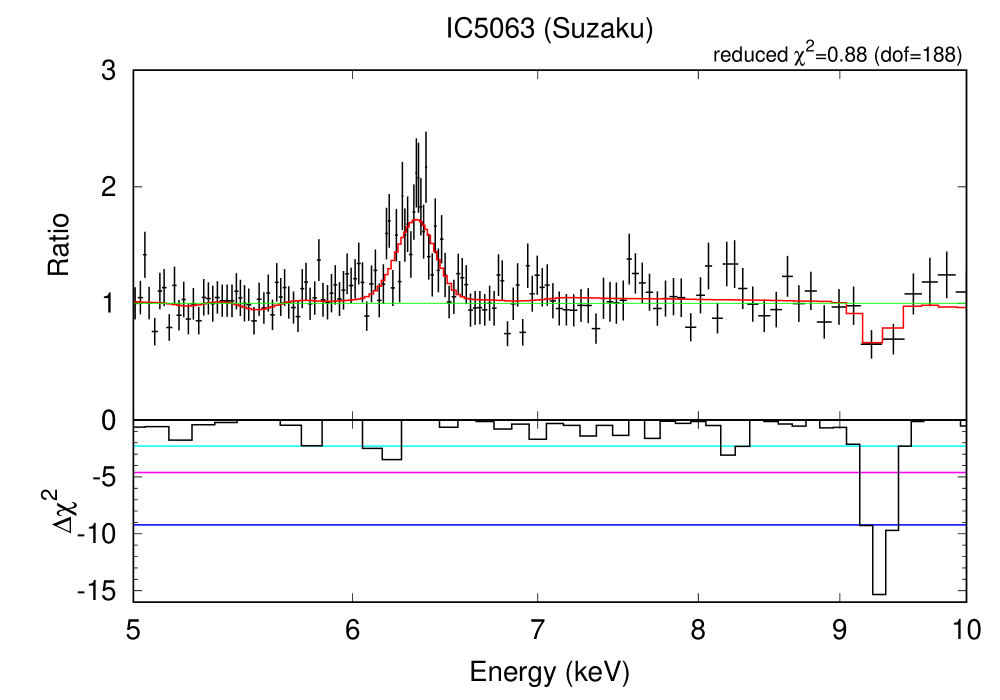
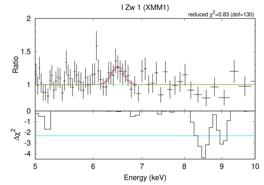
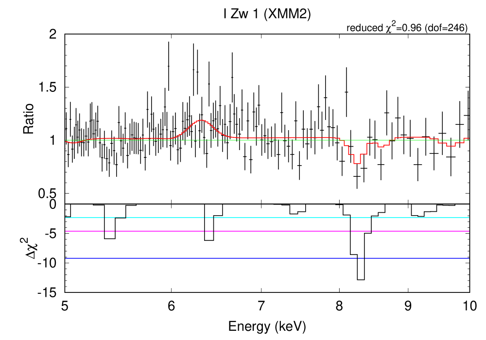
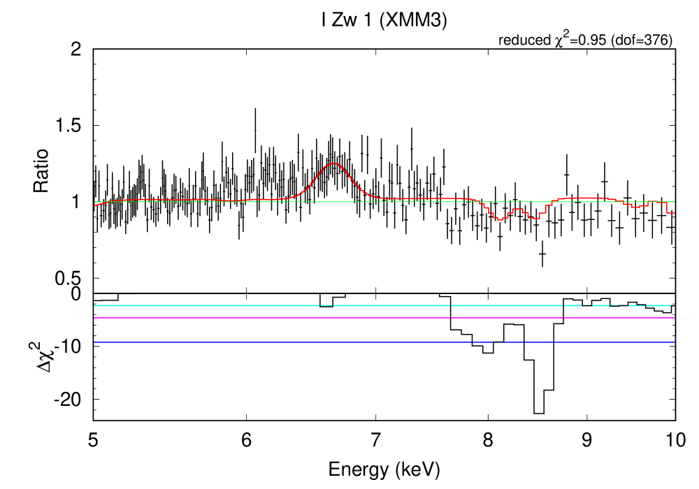
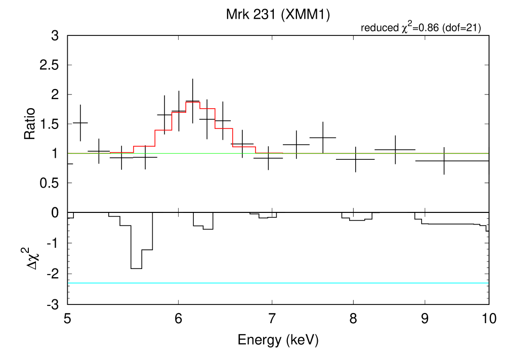
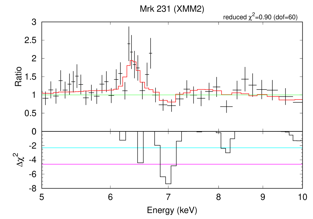
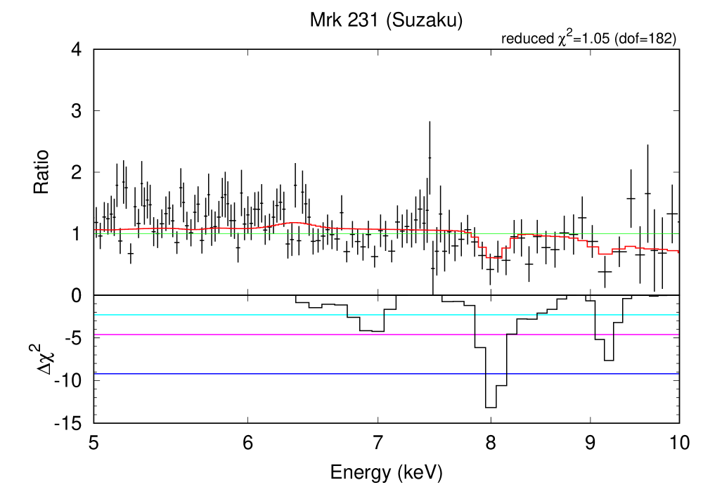
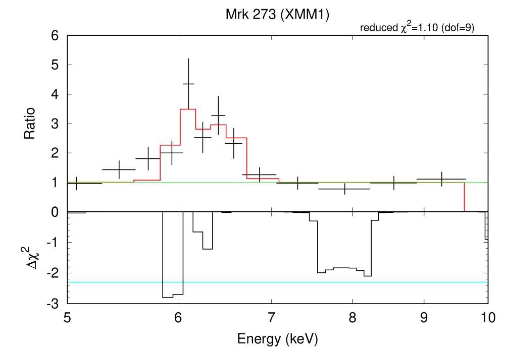
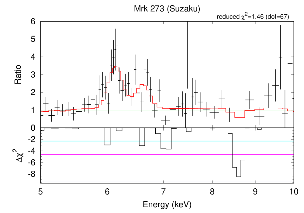
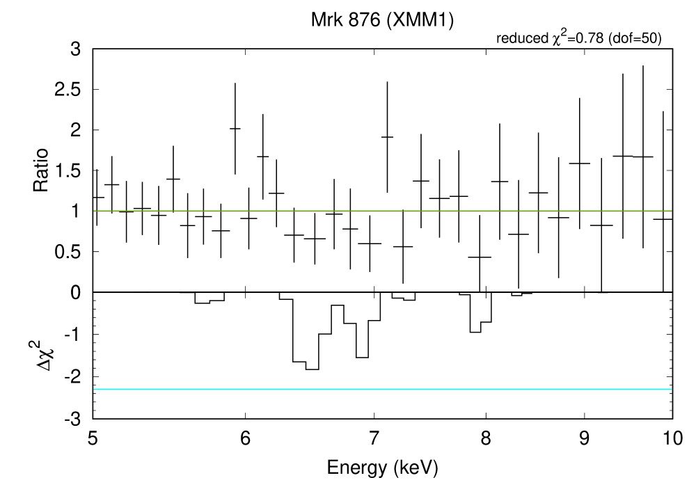
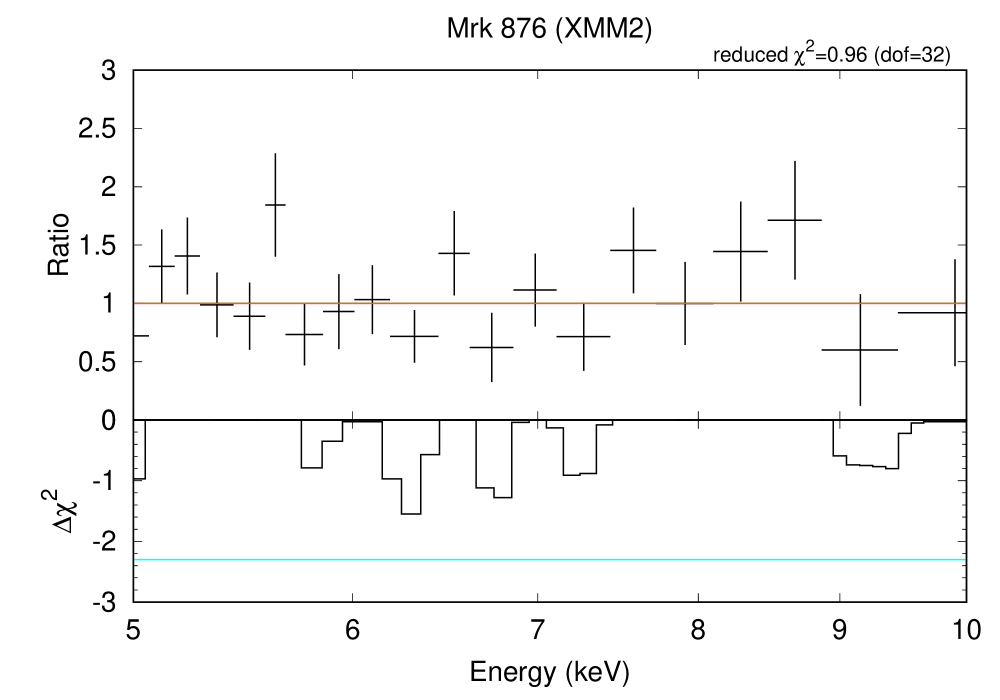
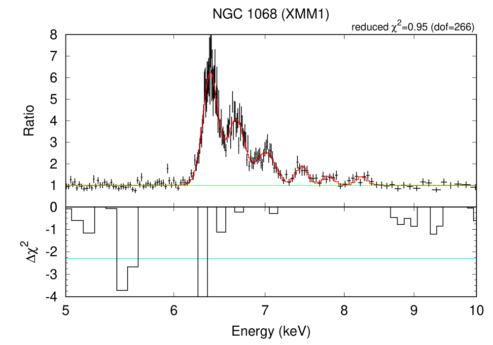
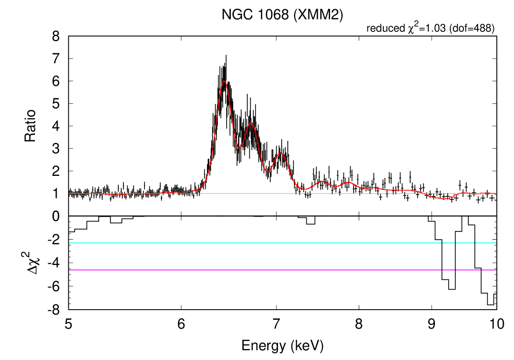
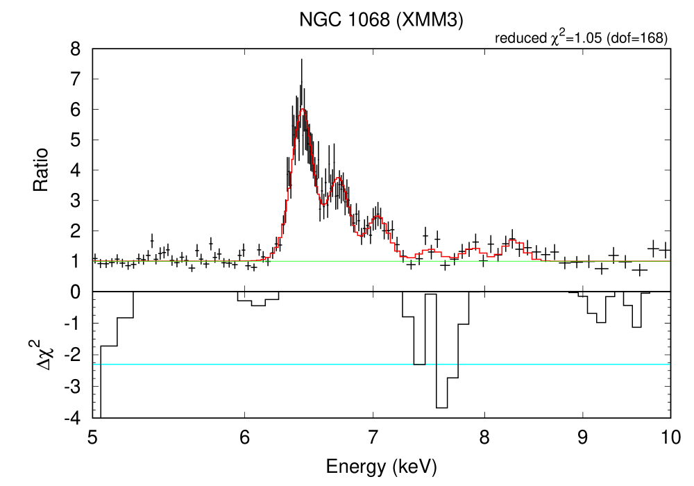
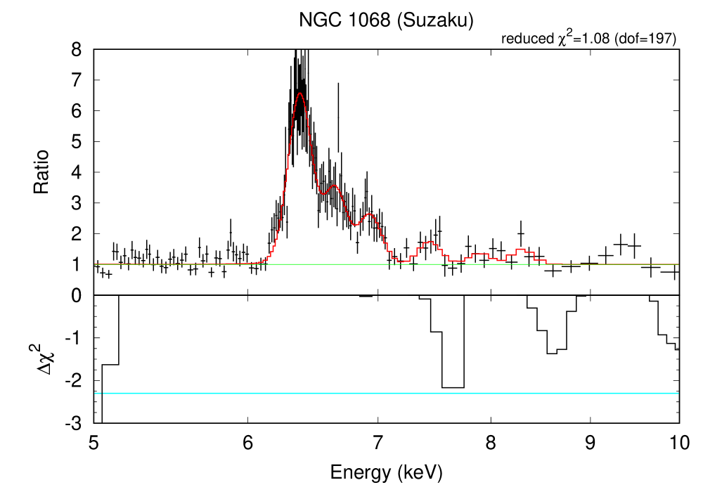
Figure 1: Top: ratio of the energy spectra to the continuum (power-law) component. The red curvatures show the fitting model. The absorption features can be seen in the red lines when the absorption lines are detected more than 90% significance level. The reduced $\chi^{2}$ and degrees of freedom are shown in the top right of each panel. Bottom: $\Delta\chi^{2}$ plots with the 68% (cyan), 90% (magenta), and 99% (blue) significance levels, from top to bottom. Only the values when the normalization of the Gaussian is negative are plotted.

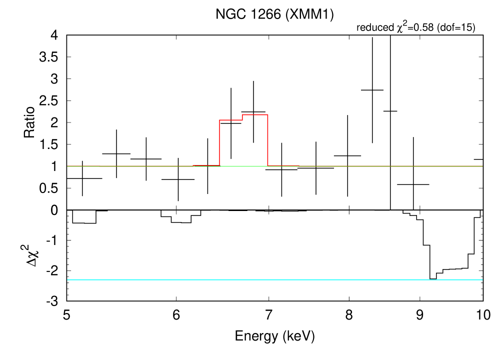
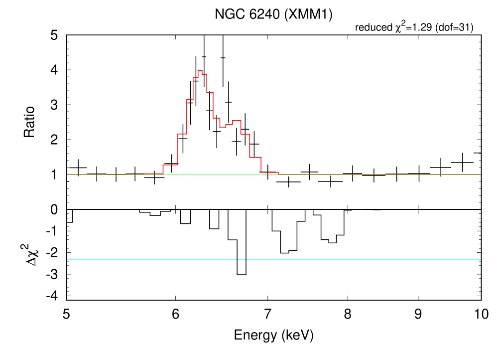
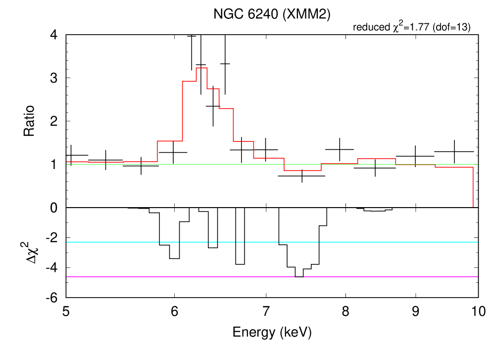
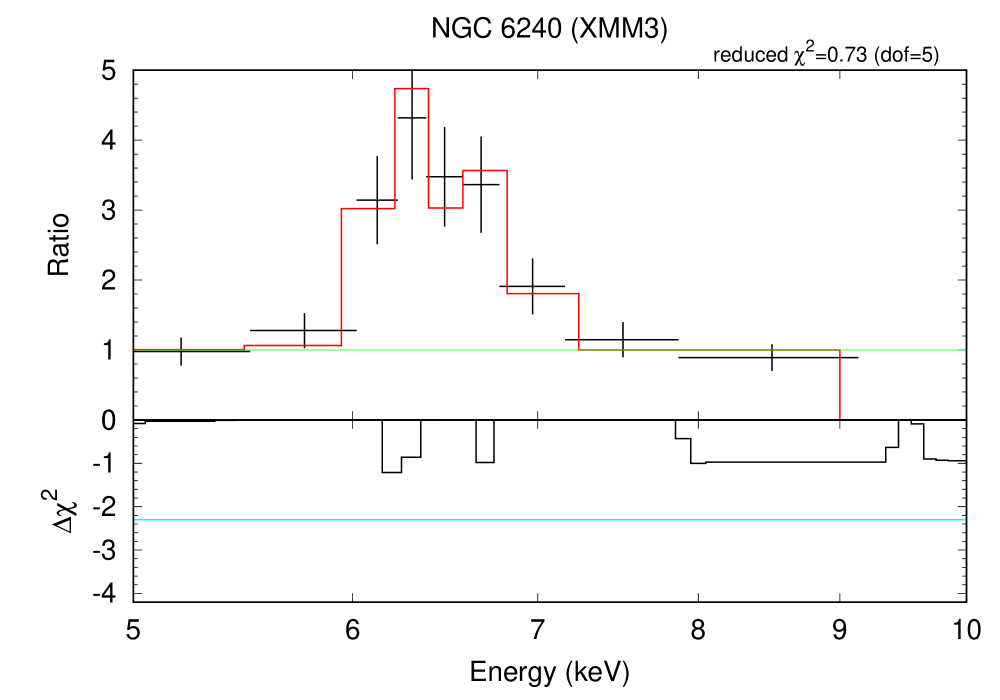
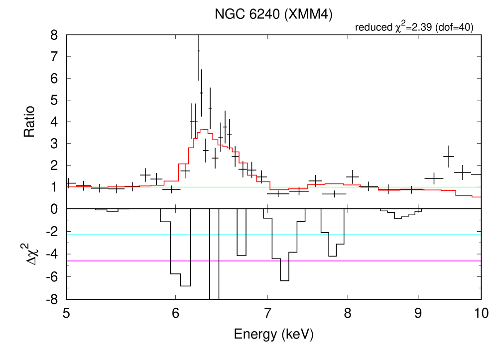
Figure 1: Continued.

The mass outflow rate, momentum, and energy-loss rate of the UFO are expressed as

$$\begin{split}\dot{M}_{\rm UFO}&\sim\Omega br^{2}m_{p}n(r)v_{\rm UFO}\\ \dot{P}_{\rm UFO}&\sim\dot{M}_{\rm UFO}v_{\rm UFO}\\ \dot{K}_{\rm UFO}&\sim\dot{M}_{\rm UFO}v^{2}_{\rm UFO}/2,\end{split}$$ (1)

where $\Omega$ is the solid angle of the wind, $b$ the volume filling factor, $m_{p}$ is the proton mass, and $n(r)$ is the electron number density (Gofford et al., 2015). They explicitly depend on $r$, which is difficult to directly constrain with the observables. In this paper, we use a conservative manner that the wind is launched at the radius where the wind velocity exceeds the escape velocity (e.g. Tombesi et al. 2015). When $v_{\rm UFO}$ equals the escape velocity $v_{\rm esc}=\sqrt{2GM_{\rm BH}/r}$, the location of the wind is written as

$$r=\frac{2GM_{\rm BH}}{v_{\rm UFO}^{2}}.$$ (2)

Please note that this radius gives a minimum value of equation (1). In this case, equation (1) are

$$\begin{split}\dot{M}_{\rm UFO}&\sim 2\Omega GM_{\rm BH}m_{p}N_{\rm H}v_{\rm UFO}^{-1}\\ \dot{P}_{\rm UFO}&\sim 2\Omega GM_{\rm BH}m_{p}N_{\rm H}\\ \dot{K}_{\rm UFO}&\sim\Omega GM_{\rm BH}m_{p}N_{\rm H}v_{\rm UFO},\end{split}$$ (3)

respectively, (see equation 3–5 in Gofford et al. 2015). We adopt $\Omega/4\pi=0.4$ as the typical and conservative value, because the detection rate of the UFO lines in the literature is about 40% (Tombesi et al., 2010; Gofford et al., 2013). The derived values in each observation are listed in table 4.

Table 4: Results of the X-ray spectral fitting of UFO lines in each data set

Object	Name	$N_{\rm H}$	$\log\xi$	$v_{\rm UFO}$	$\dot{M}_{\rm UFO}$	$\dot{P}_{\rm UFO}$	$\dot{K}_{\rm UFO}$
		(cm-2)		(km s-1)	($M_{\odot}$ yr-1)	($L_{\rm AGN}/c$)	($L_{\rm AGN}$)
IC 5063	Suzaku	$1.2_{-0.6}^{+1.2}\times 10^{23}$	$2.7_{-0.3}^{+0.2}$	$9.29_{-0.14}^{+0.13}\times 10^{4}$	$1.3_{-0.6}^{+1.3}\times 10^{-1}$	$1.2_{-0.5}^{+1.1}\times 10^{1}$	$1.8_{-0.8}^{+1.7}$
I Zw 1	XMM2	$5.0_{-4.3}^{+13.9}\times 10^{22}$	$3.6_{-1.0}^{+0.7}$	$8\pm 2\times 10^{4}$	$6.5_{-5.6}^{+18.0}\times 10^{-3}$	$4.0_{-3.4}^{+10.9}\times 10^{-2}$	$5.0_{-4.3}^{+13.7}\times 10^{-3}$
	XMM3	$2.3_{-1.9}\times 10^{23}$	$4.4_{-0.4}$	$7.1\pm 0.3\times 10^{4}$	$3.2_{-2.7}\times 10^{-2}$	$1.8_{-1.5}\times 10^{-1}$	$2.2_{-1.8}\times 10^{-2}$
Mrk 231	XMM2	$8_{-5}^{+12}\times 10^{23}$	$3.4_{-0.3}^{+0.5}$	$12.7_{-0.4}^{+1.3}\times 10^{4}$	$1.7_{-1.4}^{+2.8}\times 10^{-1}$	$1.6_{-1.1}^{+2.7}\times 10^{-1}$	$7_{-5}^{+13}\times 10^{-3}$
	Suzaku	$8_{-6}^{+22}\times 10^{22}$	$2.7\pm 0.9$	$7.0\pm 0.3\times 10^{4}$	$7_{-5}^{+19}\times 10^{-3}$	$1.6_{-1.4}^{+4.8}\times 10^{-2}$	$1.9_{-1.6}^{+5.6}\times 10^{-3}$
Mrk 273	Suzaku	$1.8_{-1.6}^{+3.1}\times 10^{24}$	$3.5_{-0.6}^{+0.9}$	$7.9\pm 0.3\times 10^{4}$	$4.5_{-3.9}^{+7.8}$	$1.3_{-1.1}^{+2.2}\times 10^{2}$	$1.6_{-1.4}^{+2.8}\times 10^{1}$
NGC 1068	XMM2	$6_{-3}^{+4}\times 10^{23}$	$3.18_{-0.09}$	$8.4_{-0.2}^{+0.3}\times 10^{4}$	$4_{-2}^{+3}\times 10^{-2}$	$7_{-4}^{+5}$	$1.0_{-0.5}^{+0.7}$
NGC 6240	XMM2	$1.8\pm 1.7\times 10^{24}$	$3.5_{-0.8}$	$4.3_{-2.6}^{+1.0}\times 10^{4}$	$3.4_{-3.3}^{+3.8}$	$1.1\pm 1.0\times 10^{1}$	$8_{-8}^{+7}\times 10^{-1}$
	XMM4	$1.8_{-1.7}^{+2.3}\times 10^{24}$	$3.1_{-0.3}^{+1.5}$	$3.2_{-0.4}^{+0.7}\times 10^{4}$	$4.6_{-4.6}^{+5.9}$	$1.1_{-1.1}^{+1.4}\times 10^{1}$	$5.9_{-5.9}^{+7.6}\times 10^{-1}$

Note. — Errors are quoted at the statistic 90% level.

Most UFOs are episodic; for example, in NGC 6240, UFO absorption lines are detected in XMM2 (exposure time is 4763 s) and XMM4 (10678 s) observations, whereas not in XMM1 (10119 s) or XMM3 (3050 s). This episodicity may be due to change of the column density, the ionization state, and/or the wind geometry (e.g. Cappi et al. 2009). Here, we assume that the mass-loss rate is zero when the UFO line is not seen because its estimation is difficult without information of the absorption line. This assumption provides us the lower limit of the mass-loss rate. In NGC 6240 case, the “time-averaged” $v_{\rm UFO}$ is calculated to be $(4.3\times 10^{4}\mathrm{\,km\,s^{-1}}\times 4763\mathrm{\,s}+3.2\times 10^{4}\mathrm{\,km\,s^{-1}}\times 10678\mathrm{\,s})/(4763\mathrm{\,s}+10678\mathrm{\,s})=3.5\times 10^{4}$ km s^-1. The average $\dot{M}_{\rm UFO}$ is calculated to be $(0\,M_{\odot}\mathrm{\,yr^{-1}}\times 10119\mathrm{\,s}+3.4\,M_{\odot}\mathrm{\,yr^{-1}}\times 4763\mathrm{\,s}+0\,M_{\odot}\mathrm{\,yr^{-1}}\times 3050\mathrm{\,s}+4.6\,M_{\odot}\mathrm{\,yr^{-1}}\times 10678\mathrm{\,s})/(10119\mathrm{\,s}+4763\mathrm{\,s}+3050\mathrm{\,s}+10678\mathrm{\,s})=2.3$ $M_{\odot}$ yr^-1. The average $\dot{P}_{\rm UFO}$ and $\dot{K}_{\rm UFO}$ are also calculated in the same way. These time-averaged parameters are listed in table 5.

Table 5: Properties of UFOs

Object	$v_{\rm UFO}$	$\dot{M}_{\rm UFO}$	$\dot{P}_{\rm UFO}$	$\dot{K}_{\rm UFO}$	$C$
	(km s-1)	($M_{\odot}$ yr-1)	$(L_{\rm AGN}/c)$	($L_{\rm AGN}$)	($=\dot{K}_{\rm mol}/\dot{K}_{\rm UFO}$)
IC 5063	$9.29_{-0.14}^{+0.13}\times 10^{4}$	$1.3_{-0.6}^{+1.3}\times 10^{-1}$	$1.2_{-0.5}^{+1.1}\times 10^{1}$	$1.8_{-0.8}^{+1.7}$	$6_{-5}^{+6}\times 10^{-3}$
I Zw 1	$7.2\pm 0.3\times 10^{4}$	$2.4_{-1.8}\times 10^{-2}$	$1.4_{-1.1}\times 10^{-1}$	$1.6_{-1.3}\times 10^{-2}$	$0.3^{+1.4}$
Mrk 231	$6.3_{-0.3}^{+0.4}\times 10^{4}$	$3.1_{-2.2}^{+4.6}\times 10^{-2}$	$3.8_{-2.0}^{+5.6}\times 10^{-2}$	$2.6_{-1.4}^{+4.7}\times 10^{-3}$	$12_{-8}^{+13}$
Mrk 273	$7.9\pm 0.3\times 10^{4}$	$3.7_{-3.2}^{+6.4}$	$1.0_{-0.9}^{1.8}\times 10^{2}$	$1.3_{-1.2}^{+2.3}\times 10^{1}$	$8_{-5}^{+2}\times 10^{-3}$
NGC 1068	$8.4_{-0.2}^{+0.3}\times 10^{4}$	$1.8_{-0.9}^{+1.3}\times 10^{-2}$	$3.4_{-1.7}^{+2.4}$	$4.8_{-2.4}^{+3.4}\times 10^{-1}$	$4_{-2}^{+8}\times 10^{-2}$
(ALMA)					$1.2_{-0.7}^{+1.3}\times 10^{-2}$
NGC 6240	$3.5_{-0.8}^{+1.0}\times 10^{4}$	$2.3_{-2.3}^{+2.8}$	$5.9_{-5.9}^{+7.0}$	$3.5_{-3.5}^{+4.1}\times 10^{-1}$	$6_{-3}\times 10^{-2}$
(ALMA)					$2.0_{-1.1}\times 10^{-2}$
IRAS F11119+3257	$7.6\pm 0.3\times 10^{4}$	1.5	$1.3_{-0.9}^{+1.7}$	$0.15$	$1.0-2.7\times 10^{-2}$

Note. — Errors are quoted at the statistic 90% level. Results of IRAS F11119+3257 are based on Tombesi et al. (2015).

Next, we compare the UFO parameters with those of the molecular outflows. Figure 2 shows momentum versus outflow velocity (also see figure 3 in Tombesi et al. 2015 and figure 6 in Feruglio et al. 2017). The horizontal line shows the momentum-conserving flow, whereas the one ascending toward the left shows the energy-conserving flow. In this figure, Mrk 231 and I Zw 1 seem to be on the energy-conserving lines, whereas Mrk 273, IC5063 are on the momentum-conserving ones. NGC 1068 and NGC 6240 are located between the two types of flows.

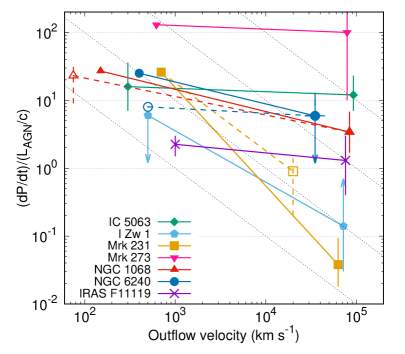
Figure 2: Momentum versus outflow velocity. The horizontal line shows the momentum-conserving flow, whereas the one ascending toward the left shows the energy-conserving flow. The opened points of NGC 1068 (triangle) and NGC 6240 (circle) show the published ALMA results, and that of Mrk 231 (square) shows the published Chandra and NuSTAR result.

The upper panel of figure 3 shows the kinetic energies versus the outflow velocities. We can see that the kinetic energies in almost all the targets (except for Mrk 231) are lost between the two outflows, which supports the idea that the molecular outflow is an accumulation of the ambient gas swept by the shock fronts UFOs have created and that radiative cooling occurs before the outflow gas reaches the shock front. The energy-transfer rate of Mrk 231 exceptionally exceeds unity; this is probably because our data picked up weak UFOs. Feruglio et al. (2015) analyzed the different data set of Mrk 231 (Chandra and NuSTAR observations), and derived the parameters of $v_{\rm UFO}=2.0_{-0.2}^{+0.3}\times 10^{4}$ km s^-1, $\dot{P}_{\rm UFO}/(L_{\rm AGN}/c)=0.2-1.6$, shown in the opened square point in figure 2 and 3. In this case, the data points are on the energy-conserving flow, i.e., $C$ is almost unity. As a result, the energy-transfer rates are distributed between $C\sim 0.007-1$ (see the bottom panel of figure 3).

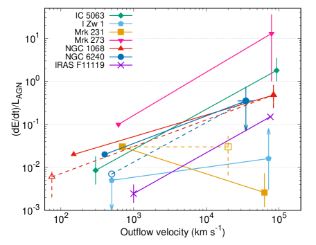
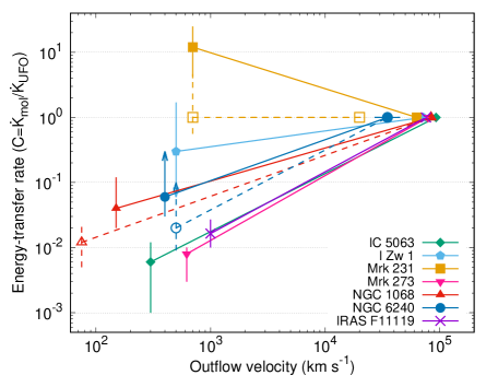
Figure 3: Kinetic energy versus outflow velocity. The vertical axis in the lower panel is normalized by the UFO kinetic energies, which corresponds to the energy-transfer rate $C$. The point types are the same as in figure 2.

4 Discussion

4.1 Parameter dependence

Figures 4 and 5 show $L_{\rm AGN}$- and $L_{\rm Edd}$ dependence of the energy-loss rates, respectively. First, in figure 4, kinetic energies of each type of outflows are expected to have positive correlation to the AGN luminosities; $\log\dot{K}_{\rm UFO}=(-23.5^{+23.6}_{-44.7})+(1.5^{+1.0}_{-0.8})\log L_{\rm AGN}$ (Gofford et al., 2015) and $\log\dot{K}_{\rm mol}=(-9.6\pm 6.1)+(1.18\pm 0.14)\log L_{\rm AGN}$ (Cicone et al., 2014). Our samples are roughly on these correlations, and both the outflows seem to share the similar dependence for the AGN luminosities. Next, in figure 5, we can see that the UFO kinetic energy has a positive correlation to the Eddington luminosities (i.e., BH masses). This correlation can be explained by equation (1), which means that larger energies are needed to escape stronger gravitational fields of heavier BH. IRAS F11119+3257 has exceptionally strong kinetic energy (the isolated blue point in the top-left side of Fig. 5), so we fit the data points except IRAS F11119+3257 with a linear function. The best-fit function is $\log(\dot{K}_{\rm UFO})=44.32\pm 0.30+(1.34\pm 0.23)(\log L_{\rm Edd}-46)$, which is shown in the blue line in Fig. 5). On the other hand, the kinetic energies of molecular outflows are almost independent of the Eddington luminosities. The best-fit linear function expect for IRAS F11119+3257 is $\log(\dot{K}_{\rm mol})=43.19\pm 0.38+(0.11\pm 0.57)(\log L_{\rm Edd}-46)$ (the red line). This implies some feedback mechanism to suppress the kinetic energy of molecular outflows to a certain value, no matter how strong the UFO is.

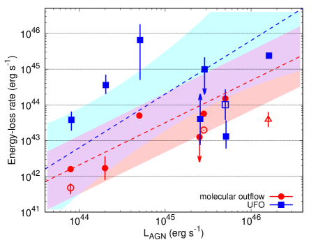
Figure 4: Energy-loss rate ($\dot{K}$) versus AGN luminosity ($L_{\rm AGN}$). The blue/red points show the UFO/molecular outflow, respectively. The red-filled circles show the IRAM data, whereas the red-open circles show the ALMA data. The red triangle shows the Herschel data of IRAS F11119+3257. The blue-filled squares show the results of this work, whereas the open one is the Chandra+NuSTAR data (Feruglio et al., 2015). The dotted lines are the best-fit linear functions for larger samples in Gofford et al. (2015) for UFO and Cicone et al. (2014) for molecular outflows, whose error ranges are shown in the shaded areas.

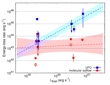
Figure 5: Energy-loss rate ($\dot{K}$) versus Eddington luminosity ($L_{\rm Edd}$). See the caption of 4 for details.

Figure 6 shows the energy-transfer rate versus BH masses. We can see negative correlation in Figure 6. The energy-transfer rate reaches unity for the small BH masses, which means that the energy-conserving shock exists. On the other hand, the momentum-conserving shock seems to exist when $M_{\rm BH}\gtrsim 5\times 10^{8}\,M_{\odot}$, i.e., $C=v_{\rm molecular}/v_{\rm UFO}\sim 500$ km s${}^{-1}/7\times 10^{4}$ km s${}^{-1}\sim 0.007$. This is the minimum $C$ value. The best-fit linear function is shown in the blue line in Fig. 6; $\log(C)=-0.96\pm 0.64+(-1.45\pm 0.88)(\log M_{\rm BH}-8)$. The black dashed line in Fig. 6 is the expected correlation, in which $0.007\leq C\leq 1$. This negative correlation means that the radiative cooling is more effective when the BH mass is larger.

King (2003) said that whether the radiative cooling is effective or not depends on the balance of the cooling time scale of the outflowing gas and the flow time scale. The cooling efficiency of the outflowing gas depends on the balance of these two time scales (King, 2003; King et al., 2011). Now we assume that the radius of the reverse shock between the unshocked UFO wind and the shocked UFO wind is small enough to be neglected and the hot bubble filled with the shocked UFO wind exists. In this case, the hot bubble is thermalized and the Compton cooling may work. King (2003) shows that the Compton cooling time of the gas in the Eddington luminosity case is

$$t_{\rm cool}=\frac{2cR^{2}}{3\pi GM_{\rm BH}}\left(\frac{m_{e}}{m_{p}}\right)^{2}\left(\frac{v}{c}\right)^{-2}b,$$ (4)

where $m_{e/p}$ is the electron/proton mass and $b(\lesssim 1)$ is the filling factor for the collimation of the wind. On the other hand, the flow time scale (for the momentum-driven case) is expressed as

$$t_{\rm flow}=R\left(\frac{2\pi G^{2}M_{\rm BH}}{f_{\rm gas}\sigma^{2}\kappa}\right)^{-1/2},$$ (5)

where $f_{\rm gas}$ is the gas fraction to the dark matter, $\sigma$ is the velocity dispersion, and $\kappa$ is the opacity. Consequently, the ratio of the two time scales is

$$\begin{split}\frac{t_{c}}{t_{f}}&=\frac{2}{3\pi}cR\left(\frac{m_{e}}{m_{p}}\right)^{2}\left(\frac{v}{c}\right)^{-2}b\left(\frac{2\pi}{M_{\rm BH}f_{\rm gas}\sigma^{2}\kappa}\right)^{1/2}\\ &\simeq 1.8\left(\frac{M_{\rm BH}}{10^{8}M_{\odot}}\right)^{-1/2}\left(\frac{R}{1\,{\rm kpc}}\right)\left(\frac{v}{0.1c}\right)^{-2}.\end{split}$$ (6)

This equation shows that the cooling is more efficient (i.e., the energy-transfer rate is smaller) for larger BH masses, which is consistent with figure 6.

Richings & Faucher-Giguère (2018a, b) performed the hydro-chemical simulations to demonstrate the molecular outflow swept by the inner outflow assuming UFO. They isotropically injected wind particles within the inner boundary with the velocity of $0.1c$, assuming a spherically symmetric geometry. They consider the radiative cooling in both the shocked UFO and the shocked ambient gas, and showed that the energy-transfer rate decreases in the higher BH masses mainly due to stronger gravitational potential. In the larger BH mass case, the velocity dispersion becomes larger and the mass of the host galaxy enclosed within $R$, which is shown as $M_{\rm gal}(<R)=2\sigma^{2}R/G$, becomes larger (see equation 2.2 in Richings & Faucher-Giguère 2018b). This tendency is also consistent with our results.

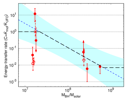
Figure 6: Energy-transfer rate ($C$) versus BH mass ($M_{\rm BH}$). The filled circles show the IRAM data of the Seyfert galaxies, whereas the open circles show the ALMA data. The cross bin is the Chandra+NuSTAR results of Mrk 231, and the open triangle shows the IRAS F11119+3257. The blue line and the cyan-shaded region show the best-fit linear function and its error range, in which only the filled circle data points are used. The black dashed line is the expected relation whose maximum is unity and minimum is $\sim 0.007$.

The other possibility is that the energy-transfer rate depends on the Eddington ratios. From figures 4 and 5, we can easily notice that the energy-transfer rate increases toward larger Eddington ratios (figure 7). The energy-transfer rate reaches maximum at around the Eddington luminosity, and minimum when $L_{\rm AGN}/L_{\rm Edd}\lesssim 10^{-2}$. The best-fit linear function is $\log(C)=0.11\pm 0.28+(1.19\pm 0.33)\log(L_{\rm AGN}/L_{\rm Edd})$. In this case, the quasar mode feedback is more efficient for Eddington/super-Eddington AGNs. However, Richings & Faucher-Giguère (2018b) shows that the energy-transfer rate is independent of AGN luminosity for the fixed $M_{\rm BH}=10^{8}M_{\odot}$, which clearly contradicts our results. Now the number of targets is very limited and the selection bias may exist; our sample has a pseudo-correlation between $M_{\rm BH}$ and $L_{\rm AGN}/L_{\rm Edd}$. More samples are needed to investigate the environmental dependence of AGN feedback more strictly. If the energy-transfer rate is large for the larger Eddington ratios, the BH mass may be fixed in the super-Eddington phase via strong accretion and strong feedback, because most of the BH masses are considered to be acquired in the super-Eddington accretion phase (Kawaguchi et al., 2004).

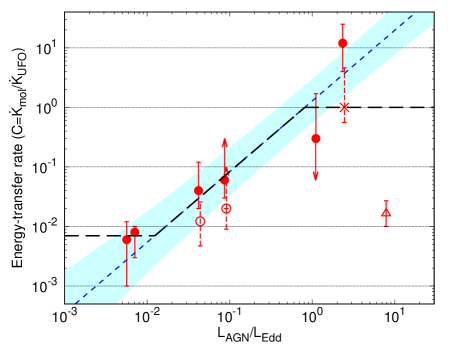
Figure 7: Energy-transfer rate ($C$) versus Eddington ratios ($L_{\rm AGN}/L_{\rm Edd}$). See the caption of figure 6 for details.

4.2 Comments on uncertainty

The energy-outflow rates of both the UFOs and molecular outflows have uncertainty. The largest uncertainty in UFO parameters is the wind geometry, which determines $\Omega$ and $r$. The X-ray reverberation lag techniques would make it possible to constrain $\Omega$ (see Mizumoto et al. 2019), but this method is not yet well established. Ratios of the triplet lines in some ions (like Si and Fe) can constrain $n$ of the X-ray absorbers, but the current grating instrument can make only a rough constraint even with the good photon statistics (e.g., $n>10^{7}$ cm^-3 for NGC 5548; Mao et al. 2017); therefore $r$ is not yet well constrained. In addition to it, the CCD calibration uncertainties have been reported; absorption-line-like features are sometimes detected at $\sim 9$ keV in the Crab data, which must have no intrinsic absorption lines in this energy band (see figure A2 in Kolehmainen et al. 2014). This means that we may misdetect UFO lines in the “featureless” X-ray energy spectra. Future missions with greater energy resolution and/or larger effective areas, such as X-Ray Imaging and Spectroscopy Mission (XRISM) and Advanced Telescope for High ENergy Astrophysics (Athena), will make it possible to detect the absorption features more confidently and let us know the detailed UFO parameters. In molecular outflows, their sizes are most difficult to constrain. Indeed, the IRAM observations in Cicone et al. (2014) estimated size of the outflowing gases with simple modeling of their visibility, and cannot see their detailed geometry. This estimation seems to overestimate the kinetic energies of molecular outflows by about three factors (see table 5). Therefore, spatially resolved observations with ALMA and IRAM (for nearby targets) are needed for more samples. Consequently, for both UFOs and molecular outflows, an increasing number of samples with less uncertainty is required for detailed studies of energy transfer in outflows.

5 Conclusion

To test whether the UFO kinetic energies are efficiently transferred into the galactic-scale molecular outflows and contribute to the AGN feedback, we investigate the energy-transfer rate for larger samples. The energy-transfer rate is defined as $C=\dot{K}_{\rm molecular}/\dot{K}_{\rm UFO}$, where $K_{i}$ is the kinetic energies of molecular outflows and UFOs. We analyzed the X-ray (XMM-Newton and Suzaku) archive data of the targets that the molecular outflows are detected in IRAM/PdBI observations listed in Cicone et al. (2014), and derived the energy-transfer rates for six Seyfert galaxies (plus type 1 quasar IRAS F11119+3257). The energy-transfer rates are distributed between 0.007 (for the momentum-conserving shock) and 1 (for the energy-conserving shock). We can see the correlation that the energy-transfer rate increases toward larger Eddington ratios (or lower BH masses), which can be explained by the balance of cooling time scale and flow time scale. Consequently, we have found that UFO contribution to the AGN feedback is effective when the Eddington ratio is large and/or BH mass is small.

References

- Cappi et al. (2009) Cappi, M., Tombesi, F., Bianchi, S., et al. 2009, A&A, 504, 401
- Cicone et al. (2012) Cicone, C., Feruglio, C., Maiolino, R., et al. 2012, A&A, 543, A99
- Cicone et al. (2014) Cicone, C., Maiolino, R., Sturm, E., et al. 2014, A&A, 562, A21
- Dasyra et al. (2006) Dasyra, K. M., Tacconi, L. J., Davies, R. I., et al. 2006, ApJ, 651, 835
- Feruglio et al. (2010) Feruglio, C., Maiolino, R., Piconcelli, E., et al. 2010, A&A, 518, L155
- Feruglio et al. (2015) Feruglio, C., Fiore, F., Carniani, S., et al. 2015, A&A, 583, A99
- Feruglio et al. (2017) Feruglio, C., Ferrara, A., Bischetti, M., et al. 2017, A&A, 608, A30
- García-Burillo et al. (2014) García-Burillo, S., Combes, F., Usero, A., et al. 2014, A&A, 567, A125
- Gofford et al. (2015) Gofford, J., Reeves, J. N., McLaughlin, D. E., et al. 2015, MNRAS, 451, 4169
- Gofford et al. (2013) Gofford, J., Reeves, J. N., Tombesi, F., et al. 2013, MNRAS, 430, 60
- Greenhill & Gwinn (1997) Greenhill, L. J., & Gwinn, C. R. 1997, Ap&SS, 248, 261
- Hamann et al. (2018) Hamann, F., Chartas, G., Reeves, J., & Nardini, E. 2018, MNRAS, 476, 943
- Honma et al. (1995) Honma, M., Sofue, Y., & Arimoto, N. 1995, A&A, 304, 1
- Jansen et al. (2001) Jansen, F., Lumb, D., Altieri, B., et al. 2001, A&A, 365, L1
- Kawaguchi et al. (2004) Kawaguchi, T., Aoki, K., Ohta, K., & Collin, S. 2004, A&A, 420, L23
- Kawakatu et al. (2007) Kawakatu, N., Imanishi, M., & Nagao, T. 2007, ApJ, 661, 660
- King (2003) King, A. 2003, ApJ, 596, L27
- King & Pounds (2015) King, A., & Pounds, K. 2015, ARA&A, 53, 115
- King & Pounds (2003) King, A. R., & Pounds, K. A. 2003, MNRAS, 345, 657
- King et al. (2011) King, A. R., Zubovas, K., & Power, C. 2011, MNRAS, 415, L6
- Kolehmainen et al. (2014) Kolehmainen, M., Done, C., & Díaz Trigo, M. 2014, MNRAS, 437, 316
- Kormendy & Ho (2013) Kormendy, J., & Ho, L. C. 2013, ARA&A, 51, 511
- Koyama et al. (2007) Koyama, K., Tsunemi, H., Dotani, T., et al. 2007, PASJ, 59, 23
- Mao et al. (2017) Mao, J., Kaastra, J. S., Mehdipour, M., et al. 2017, A&A, 607, A100
- Mitsuda et al. (2007) Mitsuda, K., Bautz, M., Inoue, H., et al. 2007, PASJ, 59, 1
- Mizumoto & Ebisawa (2017) Mizumoto, M., & Ebisawa, K. 2017, MNRAS, 466, 3259
- Mizumoto et al. (2014) Mizumoto, M., Ebisawa, K., & Sameshima, H. 2014, PASJ, 66, 122
- Mizumoto et al. (2019) Mizumoto, M., Ebisawa, K., Tsujimoto, M., et al. 2019, MNRAS, 482, 5316
- Nicastro et al. (2003) Nicastro, F., Martocchia, A., & Matt, G. 2003, ApJ, 589, L13
- Pounds & King (2013) Pounds, K. A., & King, A. R. 2013, MNRAS, 433, 1369
- Reeves et al. (2008) Reeves, J., Done, C., Pounds, K., et al. 2008, MNRAS, 385, L108