On anti bounce back boundary condition

for lattice Boltzmann schemes

François Dubois^ab, Pierre Lallemand^c, Mohamed-Mahdi Tekitek^d

^a Dpt. of Mathematics, University Paris-Sud, Bât. 425, F-91405 Orsay, France.

^b Conservatoire National des Arts et Métiers, LMSSC laboratory, F-75003 Paris, France.

^c Beijing Computational Science Research Center, Haidian District, Beijing 100094, China.

^d Dpt. Mathematics, Faculty of Sciences of Tunis, University Tunis El Manar, Tunis, Tunisia.

05 April 2019

Keywords: heat equation, linear acoustic, Taylor expansion method.

PACS numbers: 02.70.Ns, 05.20.Dd, 47.10.+g

Abstract

In this contribution, we recall the derivation of the anti bounce back boundary condition for the D2Q9 lattice Boltzmann scheme. We recall various elements of the state of the art for anti bounce back applied to linear heat and acoustics equations and in particular the possibility to take into account curved boundaries. We present an asymptotic analysis that allows an expansion of all the fields in the boundary cells. This analysis based on the Taylor expansion method confirms the well known behaviour of anti bounce back boundary for the heat equation. The analysis puts also in evidence a hidden differential boundary condition in the case of linear acoustics. Indeed, we observe discrepancies in the first layers near the boundary. To reduce these discrepancies, we propose a new boundary condition mixing bounce back for the oblique links and anti bounce back for the normal link. This boundary condition is able to enforce both pressure and tangential velocity on the boundary. Numerical tests for the Poiseuille flow illustrate our theoretical analysis and show improvements in the quality of the flow.

1)  Introduction

From the early days of Lattice Boltzmann scheme studies, boundary conditions have been the object of various proposals. In fact, two popular methods of boundary conditions are used to impose given macroscopic conditions (velocity, pressure, thermal fields, …). The first one, called “half-way” was proposed in the context of cellular automata [7]. The “half-way” approach [8], consists in using the distributions that leave the domain to define the unknown distributions by a simple reflection (called bounce back) or antireflection (called anti bounce back). In this method the physical position of the wall is located between the last internal domain node and first node beyond boundary. In [24, 16] the exact position of the physical wall is investigated for some simple problems. The second method proposed first by Zou and He [30], called “boundary on the node”, uses the projection of the given macroscopic conditions in the distribution and assumes the bounce back rule for the non-equilibrium part of the particle distribution. In this method the physical wall is located on the last node of the domain.

Here, we only focus on “half-way” boundary conditions method. In a previous work [17] a novel method of analysis, based on Taylor developments, is used for the bounce back scheme. This linear analysis gives an expansion of the macroscopic quantity, on the physical wall, as powers of the mesh size. Later in [18] a generalized bounce back boundary condition for the nine velocities two-dimensional (D2Q9) lattice Boltzmann scheme is proposed. This scheme is exact up to second order by elimination of spurious density terms (first order terms).

In this contribution, the anti bounce back boundary lattice Boltzmann scheme is investigated. This scheme is used to impose Dirichlet boundary conditions for the “thermal problem”, id est the heat equation where one scalar moment is conserved, or to impose a given pressure for a linear fluid problem. Many works proposed new boundary conditions [2, 6, 20, 25, 28] intended to yield improved accuracy compared to the anti bounce back boundary scheme.

In this paper, the D2Q9 lattice Boltzmann scheme is first briefly introduced for heat equation and acoustic system (Section 2). Then in Section 3, the anti bounce back boundary condition is presented to impose a given thermal field for thermal problem or to impose a given density/pressure for the linearized fluid. In Section 4, the scheme is analyzed using Taylor expansion for the heat equation. This asymptotic analysis gives an expansion of the conserved scalar moment which is exact up to order one. In Section 5, we present the extended anti bounce back that allows to handle curved boundaries. In Section 6, anti bounce back is analyzed for the linear fluid problem. A hidden differential boundary condition is put in evidence. In Section 7, a mixing of bounce back and anti bounce back boundary scheme [15], is used and analyzed to impose a given density and a given velocity on the physical wall. Finally in Section 8 a novel boundary scheme is introduced and analyzed to impose a given pressure and tangential velocity on the boundary. A Poiseuille test case gives convergent results.

2)  D2Q9 lattice Boltzmann scheme for heat and acoustic problems

The D2Q9 lattice Boltzmann scheme uses a set of discrete velocities described in Figure 1. A density distribution $\,f_{j}\,$ is associated to each basic velocity $\,v_{j}$. The two components and the modulus of this vector are denoted by $\,v_{jx}$, $\,v_{jy}\,$ and $\,|v_{j}|\,$ respectively. The first three moments for the density and momentum are defined according to

(1) $$\rho\,=\,\sum^{8}_{j=0}f_{j}\,=\,m_{0}\,,\,\,\,J_{x}\,=\,\sum^{8}_{j=0}v_{jx}\,f_{j}\,=\,m_{1}\,,\,\,\,J_{y}\,=\,\sum^{8}_{j=0}v_{jy}\,f_{j}\,=\,m_{2}\,.\vspace*{-7pt}$$

We complete this set of moments and construct a vector $\,m\,$ of moments $\,m_{k}\,$ using Gram-Schmidt orthogonalization and an appropriate standardization to have simple expressions of the moment matrix, as proposed in [26]:

(2) $$\left\{\begin{array}[]{l}\displaystyle\varepsilon=3\,\sum_{j=0}^{8}|v_{j}|^{2}\,f_{j}\,-4\,\,\lambda^{2}\sum_{j=0}^{8}\,f_{j}\,,\\ \displaystyle\varphi_{x}=\sum_{j=0}^{8}\big{[}(v_{jx})^{2}-(v_{jy})^{2}\big{]}\,f_{j}\,,\,\,\varphi_{y}=\sum_{j=0}^{8}v_{jx}\,v_{jy}\,\,f_{j}\,,\\ \displaystyle q_{x}=3\,\sum_{j=0}^{8}|v_{j}|^{2}\,v_{jx}\,f_{j}-5\,\lambda^{2}\,\sum_{j=0}^{8}\,v_{jx}\,f_{j}\,,\,\,q_{y}=3\,\sum_{j=0}^{8}|v_{j}|^{2}\,v_{jy}\,f_{j}-5\,\lambda^{2}\,\sum_{j=0}^{8}\,v_{jy}\,f_{j}\,,\\ \displaystyle D={9\over 2}\,\sum_{j=0}^{8}|v_{j}|^{4}\,f_{j}\,\,-\,{21\over 2}\,\lambda^{2}\,\sum_{j=0}^{8}|v_{j}|^{2}\,f_{j}\,\,\,+\,4\,\lambda^{4}\,\sum_{j=0}^{8}\,f_{j}\,.\end{array}\right.\vspace*{-7pt}$$

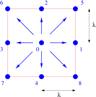
Figure 1: D2Q9 lattice Boltzmann scheme; discrete velocities $\,v_{j}\,$ for $\,0\leq j\leq 8$

The entire vector $\,m\in\mathbb{R}^{9}\,$ of moments is defined by

(3) $$m=\big{(}\rho\,,\,J_{x}\,,\,J_{y},\,\varepsilon\,,\,\varphi_{x}\,,\,\varphi_{y}\,,\,q_{x}\,,\,q_{y}\,,\,D\big{)}^{\rm\displaystyle t}\vspace*{-7pt}$$

and the previous relations can be written in a synthetic way :

(4) $$m=M\,f\,.\vspace*{-7pt}$$

The invertible fixed matrix $\,M\,$ is usually [26] given by

(5) $$M\,=\,\left(\begin{array}[]{ccccccccc}\displaystyle 1&1&1&1&1&1&1&1&1\cr\displaystyle 0&\lambda&0&-\lambda&0&\lambda&-\lambda&-\lambda&\lambda\cr\displaystyle 0&0&\lambda&0&-\lambda&\lambda&\lambda&-\lambda&-\lambda\cr\displaystyle-4\,\lambda^{2}&-\lambda^{2}&-\lambda^{2}&-\lambda^{2}&-\lambda^{2}&2\,\lambda^{2}&2\,\lambda^{2}&2\,\lambda^{2}&2\,\lambda^{2}\cr\displaystyle 0&\lambda^{2}&-\lambda^{2}&\lambda^{2}&-\lambda^{2}&0&0&0&0\cr\displaystyle 0&0&0&0&0&\lambda^{2}&-\lambda^{2}&\lambda^{2}&-\lambda^{2}\cr\displaystyle 0&-2\,\lambda^{3}&0&2\,\lambda^{3}&0&\lambda^{3}&-\lambda^{3}&-\lambda^{3}&\lambda^{3}\cr\displaystyle 0&0&-2\,\lambda^{3}&0&2\,\lambda^{3}&\lambda^{3}&\lambda^{3}&-\lambda^{3}&-\lambda^{3}\cr\displaystyle 4\,\lambda^{4}&-2\,\lambda^{4}&-2\,\lambda^{4}&-2\,\lambda^{4}&-2\,\lambda^{4}&\lambda^{4}&\lambda^{4}&\lambda^{4}&\lambda^{4}\end{array}\right)\,,\vspace*{-7pt}$$

where $\,\lambda\equiv{{\Delta x}\over{\Delta t}}\,$ is the fixed numerical lattice velocity. For scalar lattice Boltzmann applications to thermal problems, the density $\,\rho\,$ is the “conserved variable”.

$\bullet$  We suppose the following linear equilibrium of nonconserved moments and associated relaxation coefficients. Due to (5) and Table 1, we can explicit the vector $\,f^{\mathop{\rm{eq}}\nolimits}\,$ of equilibrium values of the particle distribution :

(6) $$\left\{\begin{array}[]{l}\displaystyle f_{0}^{\rm eq}={{\rho}\over{9}}\,[1-\alpha+\beta]\,,\,\,f_{1}^{\rm eq}={{\rho}\over{36}}\,[4-\alpha-2\,\beta]\,,\,\,f_{2}^{\rm eq}={{\rho}\over{36}}\,[4-\alpha-2\,\beta]\,,\\ \vspace{-4 mm}\displaystyle\\ \displaystyle f_{3}^{\rm eq}={{\rho}\over{36}}\,[4-\alpha-2\,\beta]\,,\,\,f_{4}^{\rm eq}={{\rho}\over{36}}\,[4-\alpha-2\,\beta]\,,\,\,f_{5}^{\rm eq}={{\rho}\over{36}}\,[4+2\,\alpha+\beta]\,,\\ \vspace{-4mm}\displaystyle\\ \displaystyle f_{6}^{\rm eq}={{\rho}\over{36}}\,[4+2\,\alpha+\beta]\,,\,\,f_{7}^{\rm eq}={{\rho}\over{36}}\,[4+2\,\alpha+\beta]\,,\,\,f_{8}^{\rm eq}={{\rho}\over{36}}\,[4+2\,\alpha+\beta]\,.\end{array}\right.\vspace*{-7pt}$$

moment $J_{x}$ $J_{y}$ $\varepsilon$ $\varphi_{x}$ $\varphi_{y}$ $q_{x}$ $q_{y}$ $D$ equilibrium $0$ $0$ $\alpha\,\lambda^{2}\,\rho$ $0$ $0$ $0$ $0$ $\beta\,\lambda^{4}\,\rho$ relaxation coefficient $s_{j}$ $s_{j}$ $s_{e}$ $s_{x}$ $s_{x}$ $s_{q}$ $s_{q}$ $s_{d}$

Table 1: D2Q9 linear equilibrium of nonconserved moments and associated relaxation coefficients for a thermal type problem.

$\bullet$  During the relaxation step of the heat diffusion problem, the conserved variable $\,\rho\,$ is not modified. In the framework of multiple relaxation times [23], the nonconserved moments $\,m_{1}\,$ to $\,m_{8}\,$ relax towards an equilibrium value $\,m_{k}^{\mathop{\rm{eq}}\nolimits}\,$ displayed in Table 1. The relaxation step $\,m\longrightarrow m^{*}\,$ needs also parameters $\,s_{k}\,$ presented also in the Table 1:

(7) $$m_{k}^{*}\,=\,m_{k}\,+\,s_{k}\,\big{(}m_{k}^{\mathop{\rm{eq}}\nolimits}\,-\,m_{k}\big{)}\,,\qquad k\geq 1\,.\vspace*{-7pt}$$

Companion parameters $\,\sigma_{k}\,$ have been introduced by Hénon [22] in the context of cellular automata:

$$\sigma_{k}\,=\,{{1}\over{s_{k}}}\,-\,{1\over 2}\,.\vspace*{-6pt}$$

In terms of moments, the linear collision $\,m\longrightarrow m^{*}\,$ can be written as

(8) $$m^{*}\,=\,C\,\,m\,,\vspace*{-7pt}$$

with a collision matrix $\,C\,$ given by

(9) $$\!\!\!C\!=\!\left(\begin{array}[]{ccccccccc}\!\!\!\!1&\!\!\!\!\!0&\!\!\!0&\!\!\!0&\!\!\!0&\!\!\!\!\!0&\!\!\!\!\!0&\!\!\!\!0\!\!\!\!&\!\!\!\!0\!\!\!\!\\ \!\!\!\!\!0&\!\!\!\!\!1\!\!-\!\!s_{j}&\!\!\!0&\!\!\!0&\!\!\!0&\!\!\!\!\!0&\!\!\!\!\!0&\!\!\!\!0\!\!\!\!&\!\!\!\!0\!\!\!\!\\ \!\!\!\!\!0&\!\!\!\!\!0&\!\!\!1\!\!-\!\!s_{j}&\!\!\!0&\!\!\!0&\!\!\!\!\!0&\!\!\!\!\!0&\!\!\!\!0\!\!\!\!&\!\!\!\!0\!\!\!\!\\ \!\!\!\!\!\alpha\,s_{e}\,\lambda^{2}&\!\!\!\!\!0&\!\!\!0&\!\!\!\!\!1-s_{e}&\!\!\!\!\!0&\!\!\!0&\!\!\!0&\!\!\!\!0\!\!\!\!&\!\!\!\!0\!\!\!\!\\ \!\!\!\!\!0&\!\!\!0&\!\!\!\!0&\!\!\!0&\!\!\!1-s_{x}&\!\!\!\!\!0&\!\!\!\!\!0&\!\!\!\!0\!\!\!\!&\!\!\!\!0\!\!\!\!\\ \!\!\!\!\!0&\!\!\!0&\!\!\!\!0&\!\!\!0&\!\!\!0&\!\!\!\!\!1-s_{x}&\!\!\!\!\!0&\!\!\!\!0\!\!\!\!&\!\!\!\!0\!\!\!\!\\ \!\!\!\!\!0&\!\!\!\!\!0&\!\!\!0&\!\!\!0&\!\!\!\!\!0&\!\!\!\!\!0&\!\!\!\!1-s_{q}&\!\!\!0\!\!\!\!&\!\!\!\!0\!\!\!\!\\ \!\!\!\!\!0&\!\!\!\!\!0&\!\!\!0&\!\!\!0&\!\!\!\!\!0&\!\!\!\!\!0&\!\!\!0&\!\!\!\!1-s_{q}\!\!\!\!&\!\!\!\!0\!\!\!\!\\ \beta\,s_{d}\,\lambda^{4}&\!\!\!\!\!0&\!\!\!0&\!\!\!0&\!\!\!0&\!\!\!\!\!0&\!\!\!\!\!0&\!\!\!\!0\!\!\!\!&\!\!\!\!1-s_{d}\end{array}\right)\,.\vspace*{-7pt}$$

The iteration of the D$2$Q$9$ scheme after the relaxation step follows the relation

$$f^{*}_{i}(x,\,t)\,=\,\sum_{\ell}\,M^{-1}_{i\,\ell}\,m_{\ell}^{*}\,,\,\,0\,\leq\,i\,\leq\,8\,\vspace*{-6pt}$$

and the population $\,f_{j}(x,\,t+\Delta t)\,$ ($0\leq j\leq 8$) at the new time step is evaluated according to

(10) $$f_{j}(x,t+\Delta t)\,=\,f^{*}_{j}(x-v_{j}\Delta t,t)\,,\,\,0\leq j\leq 8\,.\vspace*{-7pt}$$

$\bullet$  In [12] and [13], we have introduced classical Taylor expansions in order to recover equivalent partial differential equations of the previous internal scheme. For the thermal model, when $\,\Delta x\,$ and $\,\Delta t\,$ tend to zero, with a fixed ratio $\,\lambda\equiv{{\Delta x}\over{\Delta t}}\,$ and fixed relaxation coefficients $\,s_{k}$, the conserved variable $\,\rho\,$ is solution of an asymptotic heat equation

(11) $${{\partial\rho}\over{\partial t}}-\,\mu\,\Delta\rho={\rm O}(\Delta x^{2})\,.\vspace*{-7pt}$$

The infinitesimal diffusivity $\,\mu\,$ is evaluated according to

$$\mu={1\over 6}\,\sigma_{j}\,(\alpha+4)\,\lambda\,\Delta x\,.\vspace*{-6pt}$$

$\bullet$  If we consider a linear fluid problem, the three first moments $\,\rho$, $\,J_{x}\equiv\rho\,u_{x}\,$ and $\,J_{y}\equiv\rho\,u_{y}\,$ are conserved during the collision step. The table of equilibria and relaxation coefficients is modified in the way specified in Table 2:

moment $\varepsilon$ $\varphi_{x}$ $\varphi_{y}$ $q_{x}$ $q_{y}$ $D$ equilibrium $\alpha\,\lambda^{2}\,\rho$ $0$ $0$ $-\lambda^{2}\,J_{x}$ $-\lambda^{2}\,J_{y}$ $\beta\,\lambda^{4}\,\rho$ relaxation coefficient $s_{e}$ $s_{x}$ $s_{x}$ $s_{q}$ $s_{q}$ $s_{d}$

Table 2: D2Q9 linear equilibrium of nonconserved moments and associated relaxation coefficients for a acoustic linear fluid problem.

We can also display for the linear fluid case all components of the linear vector $\,f^{\mathop{\rm{eq}}\nolimits}$:

(12) $$\left\{\begin{array}[]{l}\displaystyle f_{0}^{\rm eq}={{\rho}\over{9}}\,[1-\alpha+\beta\,]\,,\\ \vspace{-5 mm}\displaystyle\\ \displaystyle f_{1}^{\rm eq}={{\rho}\over{36}}\,[4-\alpha-2\,\beta+{{12\,u_{x}}\over{\lambda}}]\,,\,\,f_{2}^{\rm eq}={{\rho}\over{36}}\,\,\,[4-\alpha-2\,\beta+{{12\,u_{y}}\over{\lambda}}]\,,\\ \vspace{-4 mm}\displaystyle\\ \displaystyle f_{3}^{\rm eq}={{\rho}\over{36}}\,[4-\alpha-2\,\beta-{{12\,u_{x}}\over{\lambda}}]\,,\,\,f_{4}^{\rm eq}={{\rho}\over{36}}\,[4-\alpha-2\,\beta-{{12\,u_{y}}\over{\lambda}}]\,,\\ \vspace{-4 mm}\displaystyle\\ \displaystyle f_{5}^{\rm eq}={{\rho}\over{36}}\,[4+2\,\alpha+\beta+{{3}\over{\lambda}}(u_{x}+u_{y})]\,,\,\,f_{6}^{\rm eq}={{\rho}\over{36}}\,[4+2\,\alpha+\beta+{{3}\over{\lambda}}(-u_{x}+u_{y})]\,,\\ \vspace{-4 mm}\displaystyle\\ \displaystyle f_{7}^{\rm eq}={{\rho}\over{36}}\,[4+2\,\alpha+\beta+{{3}\over{\lambda}}(-u_{x}-u_{y})]\,,\,\,f_{8}^{\rm eq}={{\rho}\over{36}}\,\,\,[4+2\,\alpha+\beta+{{3}\over{\lambda}}(u_{x}-u_{y})]\,.\end{array}\right.\vspace*{-7pt}$$

In the space of moments, the linear collision is still described by a collision matrix. In the fluid case, we have

(13) $$\!\!\!C\!=\!\left(\begin{array}[]{ccccccccc}\!\!\!\!1&\!\!\!\!\!0&\!\!\!0&\!\!\!0&\!\!\!0&\!\!\!\!\!0&\!\!\!\!\!0&\!\!\!\!0\!\!\!\!&\!\!\!\!0\!\!\!\!\\ \!\!\!\!\!0&\!\!\!\!\!1&\!\!\!0&\!\!\!0&\!\!\!0&\!\!\!\!\!0&\!\!\!\!\!0&\!\!\!\!0\!\!\!\!&\!\!\!\!0\!\!\!\!\\ \!\!\!\!\!0&\!\!\!\!\!0&\!\!\!1&\!\!\!0&\!\!\!0&\!\!\!\!\!0&\!\!\!\!\!0&\!\!\!\!0\!\!\!\!&\!\!\!\!0\!\!\!\!\\ \!\!\!\!\!\alpha\,s_{e}\,\lambda^{2}&\!\!\!\!\!0&\!\!\!0&\!\!\!\!\!1-s_{e}&\!\!\!\!\!0&\!\!\!0&\!\!\!0&\!\!\!\!0\!\!\!\!&\!\!\!\!0\!\!\!\!\\ \!\!\!\!\!0&\!\!\!0&\!\!\!\!0&\!\!\!0&\!\!\!1-s_{x}&\!\!\!\!\!0&\!\!\!\!\!0&\!\!\!\!0\!\!\!\!&\!\!\!\!0\!\!\!\!\\ \!\!\!\!\!0&\!\!\!0&\!\!\!\!0&\!\!\!0&\!\!\!0&\!\!\!\!\!1-s_{x}&\!\!\!\!\!0&\!\!\!\!0\!\!\!\!&\!\!\!\!0\!\!\!\!\\ \!\!\!\!\!0&\!\!\!\!\!-s_{q}\,\lambda^{2}&\!\!\!0&\!\!\!0&\!\!\!\!\!0&\!\!\!\!\!0&\!\!\!\!1-s_{q}&\!\!\!0\!\!\!\!&\!\!\!\!0\!\!\!\!\\ \!\!\!\!\!0&\!\!\!\!\!0&\!\!\!-s_{q}\,\lambda^{2}&\!\!\!0&\!\!\!\!\!0&\!\!\!\!\!0&\!\!\!0&\!\!\!\!1-s_{q}\!\!\!\!&\!\!\!\!0\!\!\!\!\\ \beta\,s_{d}\,\lambda^{4}&\!\!\!\!\!0&\!\!\!0&\!\!\!0&\!\!\!0&\!\!\!\!\!0&\!\!\!\!\!0&\!\!\!\!0\!\!\!\!&\!\!\!\!1-s_{d}\end{array}\right)\,.\vspace*{-7pt}$$

The sound velocity satisfies

$$c_{0}^{2}={{\alpha+4}\over{6}}\,\lambda^{2}\,.\vspace*{-6pt}$$

The shear and bulk kinematic viscosities $\,\nu\,$ and $\,\zeta\,$ are given [26] according to the relations

$$\nu={{\lambda}\over{3}}\,\Delta x\,\Big{(}{{1}\over{s_{x}}}-{1\over 2}\Big{)}\,,\quad\zeta=-{{\lambda}\alpha\over{6}}\,\Delta x\,\Big{(}{{1}\over{s_{e}}}-{1\over 2}\Big{)}\,.\vspace*{-6pt}$$

Note the usual values of the parameters : $\,\alpha=-2\,$ and $\,\beta=1$. During the relaxation step, the conserved variables $\,W\equiv(\rho\,,\,J_{x}\,,\,J_{y})\,$ are not modified. The non-conserved moments follow a relaxation algorithm described in (7).

3)  Construction of the anti bounce back boundary condition

Consider to fix the ideas a bottom boundary for the D2Q9 lattice Boltzmann scheme, as illustrated in Figure 2. For an internal node $\,x$, the evolution of populations $\,f_{j}\,$ is given by the internal scheme (10). For a bottom boundary, the values of $\,f_{j}^{*}(x-v_{j}\Delta t)\,$ for $\,j\in\{2,5,6\}\equiv\mathcal{B}\,$ are a priori unknown.

Figure 2: The issue of choosing a boundary algorithm for the D2Q9 lattice Boltzmann scheme

When the vertex $\,x\,$ is near the boundary, and located half a mesh size from the physical boundary, the internal iteration (10) is still applicable for the discrete velocities with numbers $\,j=0,\,1,\,3,\,4,\,7,\,8$, id est for $\,j\not\in\mathcal{B}$. For $\,j\in\mathcal{B}$, the fundamental scheme (10) has to be adapted. Our framework is still to try to apply the internal scheme at the boundary. In our case, we set

$$\left\{\begin{array}[]{l}f_{5}(x,t+\Delta t)=f^{*}_{5}(x-(\Delta x,\,\Delta x),t)\,,\\ f_{2}(x,t+\Delta t)=f^{*}_{2}(x-(0,\,\Delta x),t)\,,\\ f_{6}(x,t+\Delta t)=f^{*}_{6}(x+(\Delta x,\,-\Delta x),t)\,.\end{array}\right.\vspace*{-6pt}$$

Therefore, the boundary scheme is replaced by an extrapolation problem: how to determine the values $\,f_{j}^{*}(x-v_{j}\,\Delta t,\,t)\,$ for $\,j\in\mathcal{B}\,$ from the known values $\,f_{k}^{*}(x,\,t)\,$ at the given vertex $\,x\,$ and the extra information given by the boundary conditions imposed by the physics?

$\bullet$  For the thermal case, the construction of the lattice Boltzmann scheme is based on two arguments. First we can approximate at first order of accuracy (see e.g. [12]) the values $\,f_{j}^{*}(x-v_{j}\Delta t,\,t)\,$ at the neighbouring vertices by the equilibrium values $\,f_{j}^{\rm eq}(x,\,t)\,$ at the internal vertex. Second, we have from the relations (6) the following three elementary remarks: $\,f_{2}^{\rm eq}={{\rho}\over{36}}\,(4-\alpha-2\,\beta)$, $\,f_{4}^{\rm eq}={{\rho}\over{36}}\,(4-\alpha-2\,\beta)\,$ and in consequence $\,f_{2}^{\rm eq}+f_{4}^{\rm eq}={{4-\alpha-2\,\beta}\over{18}}\,\rho$. In a similar way, $\,f_{5}^{\rm eq}={{\rho}\over{36}}\,(4+2\,\alpha+\beta)\,$ and $\,f_{7}^{\rm eq}={{\rho}\over{36}}\,(4+2\,\alpha+\beta)\,$ implies $\,f_{5}^{\rm eq}+f_{7}^{\rm eq}={{4+2\,\alpha+\beta}\over{18}}\,\rho$. Last but not least, the relations $\,f_{6}^{\rm eq}={{\rho}\over{36}}\,(4+2\,\alpha+\beta)\,$ and $\,f_{8}^{\rm eq}={{\rho}\over{36}}\,(4+2\,\alpha+\beta)\,$ show that $\,f_{6}^{\rm eq}+f_{8}^{\rm eq}={{4+2\,\alpha+\beta}\over{18}}\,\rho$. If we suppose a Dirichlet boundary condition for the heat equation (11) then the conserved “temperature” $\,\rho=\rho_{0}\,$ is given on the boundary. The anti bounce back boundary condition is obtained by replacing in the previous relations the equilibrium values by the outgoing particle distribution and the moment $\,\rho(x)\,$ by the given value $\,\rho_{0}\,$ on the boundary, as illustrated in Figure 3.

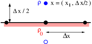
Figure 3: Cell center framework for the boundary conditions: given boundary value $\,\rho_{0}$ and conserved moment $\,\rho\,$ in the flow at vertex $\,x$.

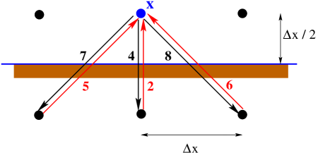
Figure 4: For a boundary node $\,x\,$ along an horizontal frontier, the D2Q9 lattice Boltzmann scheme takes into account the three numbers $\,\rho_{0}(x-{{\Delta x}\over{2}},\,t)$, $\,\rho_{0}(x,\,t)\,$ and $\,\rho_{0}(x+{{\Delta x}\over{2}},\,t)$.

The fluid node $\,x\,$ near the boundary has coordinates equal to $\,(x_{1},{{\Delta x}\over{2}})\,$ as depicted in Figure 3. In order to be more precise, we observe (see Figure 4) that the diagonal particles (numbered by $\,j=5\,$ and $\,j=6$) cross the boundary at locations $\,x_{1}-{{\Delta x}\over{2}}\,$ and $\,x_{1}+{{\Delta x}\over{2}}\,$ respectively. If we have a continuous information for the given field on the boundary, we can introduce in the boundary scheme the exact values $\,\rho_{0}(x_{1}-{{\Delta x}\over{2}},\,t)$, $\,\rho_{0}(x_{1},\,t)\,$ and $\,\rho_{0}(x_{1}+{{\Delta x}\over{2}},\,t)\,$ of the given data. Taking into account all the previous remarks, the anti bounce back boundary condition is written in this case

(14) $$\left\{\begin{array}[]{l}\displaystyle f_{5}(x,\,t+\Delta t)=-f^{*}_{7}(x,\,t)\,+\,{{4+2\,\alpha+\beta}\over{18}}\,\rho_{0}\Big{(}x_{1}-\frac{\Delta x}{2},\,t\Big{)}\,,\\ \vspace{-4 mm}\\ \displaystyle f_{2}(x,\,t+\Delta t)=-f^{*}_{4}(x,\,t)\,+\,{{4-\alpha-2\,\beta}\over{18}}\,\rho_{0}\big{(}x_{1},\,t\big{)}\,,\\ \vspace{-4 mm}\\ \displaystyle\displaystyle f_{6}(x,\,t+\Delta t)=-f^{*}_{8}(x,\,t)\,+\,{{4+2\,\alpha+\beta}\over{18}}\,\rho_{0}\Big{(}x_{1}+\frac{\Delta x}{2},\,t\Big{)}\,.\end{array}\right.\vspace*{-7pt}$$

The minus sign in the right hand side of the relations (14) characterizes the denomination of “anti” bounce back.

$\bullet$  For the linearized fluid, we have three conserved moments: density $\,\rho\,$ and the two components of the momentum $\,J\equiv\rho\,u$. The equilibrium of the particle distribution is now given by the relation (12). We have as previously three simple remarks. First, $\,f_{2}^{\rm eq}={{\rho}\over{36}}\,\big{(}4-\alpha-2\,\beta+{{12\,u_{y}}\over{\lambda}}\big{)}\,$ and $\,f_{4}^{\rm eq}={{\rho}\over{36}}\,\big{(}4-\alpha-2\,\beta-{{12\,u_{y}}\over{\lambda}}\big{)}$. In consequence, $\,f_{2}^{\rm eq}+f_{4}^{\rm eq}={{4-\alpha-2\,\beta}\over{18}}\,\rho$. Secondly, $\,f_{5}^{\rm eq}={{\rho}\over{36}}\,\big{(}4+2\,\alpha+\beta+{{3}\over{\lambda}}(u_{x}+u_{y})\big{)}\,$ and $\,f_{7}^{\rm eq}={{\rho}\over{36}}\,\big{(}4+2\,\alpha+\beta+{{3}\over{\lambda}}(-u_{x}-u_{y})\big{)}$. After a simple addition of these two expressions, $\,f_{5}^{\rm eq}+f_{7}^{\rm eq}={{4+2\,\alpha+\beta}\over{18}}\,\rho$. Finally, the relations $\,f_{6}^{\rm eq}={{\rho}\over{36}}\,\big{(}4+2\,\alpha+\beta+{{3}\over{\lambda}}(-u_{x}+u_{y})\big{)}\,$ and $\,f_{8}^{\rm eq}={{\rho}\over{36}}\,\big{(}4+2\,\alpha+\beta+{{3}\over{\lambda}}(u_{x}-u_{y})\big{)}\,$ show that $\,f_{6}^{\rm eq}+f_{8}^{\rm eq}={{4+2\,\alpha+\beta}\over{18}}\,\rho$. Applying the same method as in the case of the thermal variant of the D2Q9 lattice Boltzmann scheme, we can write the anti bounce back boundary condition again with the relations (14). The interpretation of the variable $\,\rho\,$ is now the density. The anti bounce back is associated to a pressure datum, thanks to the acoustic hypothesis that $\,p=c_{0}^{2}\,\rho$. Observe that in the fluid case, the bounce back boundary condition is obtained simply by reversing the signs: $\,f_{2}^{\rm eq}-f_{4}^{\rm eq}={{2}\over{3\,\lambda}}\,\rho\,u_{y}$, $\,f_{5}^{\rm eq}-f_{7}^{\rm eq}={{\rho}\over{6\,\lambda}}(u_{x}+u_{y})\,$ and $\,f_{6}^{\rm eq}-f_{8}^{\rm eq}={{\rho}\over{6\,\lambda}}(-u_{x}+u_{y})$.

4)  Linear asymptotic analysis for the heat problem

In order to analyze the anti bounce back boundary condition (14), we can rewrite this condition as

$$f^{*}_{j}(x,\,t)=-f^{*}_{\ell}(x,t)+\xi_{j}(x_{j}^{\prime},t)\,,\quad j\in\mathcal{B}\,,\vspace*{-6pt}$$

with $\,\mathcal{B}=\{2,\,5,\,6\}\,$ in our example. As previously the notation $\,\ell\,$ corresponds to the opposite direction of the direction number $\,j$: $\,v_{j}+v_{\ell}=0$. The expression $\,\xi_{j}(x_{j}^{\prime},t)\,$ denotes the given “temperature” $\,\rho_{0}\,$ on the boundary at the space location $\,x_{j}^{\prime}$. In the specific example considered here, we have

(15) $$\left\{\begin{array}[]{l}\displaystyle\xi_{2}(x_{2}^{\prime},\,t)={{4-\alpha-2\,\beta}\over{18}}\,\rho_{0}\big{(}x_{1},\,t)\,,\\ \vspace{-4 mm}\\ \displaystyle\xi_{5}(x_{5}^{\prime},\,t)={{4+2\,\alpha+\beta}\over{18}}\,\rho_{0}\Big{(}x_{1}-\frac{\Delta x}{2},\,t\Big{)}\,,\\ \vspace{-4 mm}\\ \displaystyle\xi_{6}(x_{6}^{\prime},\,t)={{4+2\,\alpha+\beta}\over{18}}\,\rho_{0}\Big{(}x_{1}+\frac{\Delta x}{2},\,t\Big{)}\,.\end{array}\right.\vspace*{-7pt}$$

If $\,j\notin\mathcal{B}\,$ the above equation is replaced by the internal scheme:

$$f_{j}(x,t+\Delta t)=f^{*}_{j}(x-v_{j}\Delta t,t)\,,\quad j=0,\,1,\,3,\,4,\,7,\,8\,.\vspace*{-6pt}$$

We have proposed in [17] a unified expression of the lattice Boltzmann scheme D2Q9 for a vertex $\,x\,$ near the boundary. With the help of matrices $\,T_{j,\ell}\,$ and $\,U_{j,\ell}$, we can write

(16) $$f_{j}(x,t+\Delta t)=\sum_{\ell}T_{j,\ell}\,f_{\ell}^{*}(x,t)+\sum_{\ell}U_{j,\ell}\,f^{*}_{\ell}(x-v_{j}\Delta t,t)+\xi_{j}(x_{j}^{\prime},\,t)\,,\,\,0\leq j\leq 8\,.\vspace*{-7pt}$$

The matrix element $\,U_{j,\ell}\,$ is equal to $\,1\,$ if $\,\ell=j\notin\mathcal{B}\,$ and $\,U_{j,\ell}=0\,$ if not:

(17) $$U=\left(\begin{array}[]{ccccccccc}{1}&0&0&0&0&0&0&0&0\\ 0&{1}&0&0&0&0&0&0&0\\ 0&0&0&0&0&0&0&0&0\\ 0&0&0&{1}&0&0&0&0&0\\ 0&0&0&0&{1}&0&0&0&0\\ 0&0&0&0&0&0&0&0&0\\ 0&0&0&0&0&0&0&0&0\\ 0&0&0&0&0&0&0&{1}&0\\ 0&0&0&0&0&0&0&0&{1}\end{array}\right)\,.\vspace*{-7pt}$$

In an analogous way, the explicitation of the opposite directions $\,(5,\,7)$, $\,(2,\,4)\,$ and $\,(6,\,8)\,$ leads to the following matrix denoted by $\,T_{,}$ in the relation (16):

(18) $$T=\left(\begin{array}[]{ccccccccc}0&0&0&0&0&0&0&0&0\\ 0&0&0&0&0&0&0&0&0\\ 0&0&0&0&\!-1&0&0&0&0\\ 0&0&0&0&0&0&0&0&0\\ 0&0&0&0&0&0&0&0&0\\ 0&0&0&0&0&0&0&\!-1&0\\ 0&0&0&0&0&0&0&0&\!-1\\ 0&0&0&0&0&0&0&0&0\\ 0&0&0&0&0&0&0&0&0\end{array}\right)\,.\vspace*{-7pt}$$

A complete picture of the boundary scheme is presented in Figure 5.

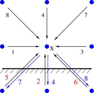
Figure 5: Vertex $\,x\,$ near a boundary for the D2Q9 lattice Boltzmann scheme

$\bullet$  The formal asymptotic analysis for infinitesimal space step $\,\Delta x\,$ and infinitesimal time step $\,\Delta t\,$ is conducted as follows. Multiply the relations (16) by the matrix $\,M\,$ of (5) in order to introduce the moments (4). Thus a complete expression of the D2Q9 lattice Boltzmann scheme for a node $\,x\,$ near the boundary takes the form

$$m_{k}(x,t+\Delta t)=(MTM^{-1}C)_{k,\ell}\ m_{\ell}(x,t)+(M_{k,\ell}\,U_{\ell,j}\,M^{-1}_{j,p}\,C_{p,q})\ m_{q}(x-v_{\ell}\Delta t,t)+M_{k,\ell}\,\xi_{\ell}\,.\vspace*{-6pt}$$

Then expand this relation at order 0 and 1. At order zero, we have

$$m_{k}+{\rm{O}}(\Delta t)=(MTM^{-1}C)_{k,\ell}\ m_{\ell}+(MUM^{-1}C)_{k,\ell}\ m_{\ell}+{\rm{O}}(\Delta x)+M_{k,\ell}\,\xi_{\ell}\,.\vspace*{-6pt}$$

Drop away the indices:

$$m+{\rm{O}}(\Delta t)=(MTM^{-1}C)\,\ m+(MUM^{-1}C)\,m+M\,\xi+{\rm{O}}(\Delta x)\,.\vspace*{-6pt}$$

We make a hypothesis of acoustic scaling: the ratio $\,{{\Delta x}\over{\Delta t}}\,$ is maintained constant as $\,\Delta x\,$ and $\,\Delta t\,$ tend to zero. We put also all the unknowns in the left hand side:

$$\big{(}I-M(T+U)M^{-1}C\big{)}\,m=M\,\xi+{\rm{O}}(\Delta x)\,.\vspace*{-6pt}$$

We introduce the matrix $\,K\,$ according to

(19) $$K\equiv I-M(T+U)M^{-1}C\,.\vspace*{-7pt}$$

We have established asymptotic equations for the moments $\,m\,$ in the first cell of the computational domain for anti bounce back scheme at order zero:

(20) $$K\,m\,=\,M\,\xi+{\rm{O}}(\Delta x)\,.\vspace*{-7pt}$$

with

$$\xi=\xi_{0}+\Delta t\,\partial\xi+{\rm{O}}(\Delta x^{2})\,.\vspace*{-6pt}$$

$\bullet$  For the anti bounce back for the thermal D$2$Q$9$ scheme, we have:

(21) $${K=\left(\begin{array}[]{ccccccccc}\!\!\!\!{1\over 6}(4+\alpha s_{e})&\!\!\!0&\!\!\!\!0&\!\!\!\!{1\over{6\lambda^{2}}}(1-s_{e})&\!\!\!\!{{1}\over{2\lambda^{2}}}(s_{x}-1)&\!\!\!\!\!\!\!0&\!\!\!\!0&\!\!\!\!0&\!\!\!\!0\\ \!\!\!\!0&\!\!\!\!s_{j}&\!\!\!\!0&\!\!\!\!0&\!\!\!\!0&\!\!\!\!{{1}\over{\lambda}}(1-s_{x})&\!\!\!\!0&\!\!\!\!0&\!\!\!\!0\\ \!\!\!\!{{\lambda}\over{6}}(4+\alpha s_{e})&\!\!\!\!0&\!\!\!\!s_{j}&\!\!\!\!{{1}\over{6\lambda}}(1-s_{e})&\!\!\!\!{{1}\over{2\,\lambda}}(s_{x}-1)&\!\!\!\!\!\!\!0&\!\!\!\!0&\!\!\!\!0&\!\!\!\!0\\ \!\!\!\!{{\lambda^{2}}\over{6}}(4-3\alpha s_{e}+2\beta s_{d})&\!\!\!\!0&\!\!\!\!0&\!\!\!\!{{1}\over{2}}(s_{e}+1)&\!\!\!\!{{1}\over{2}}(1-s_{x})&\!\!\!\!\!\!\!0&\!\!\!\!0&\!\!\!\!0&\!\!\!\!{{1}\over{3\lambda^{2}}}(1-s_{d})\\ \vspace{-.5 cm}\hfil\\ \!\!\!\!{{\lambda^{2}}\over{18}}(-4+\alpha s_{e}+2\beta s_{d})&\!\!\!\!0&\!\!\!\!0&\!\!\!\!{{1}\over{18}}(1-s_{e})&\!\!\!\!{{1}\over{2}}(1+s_{x})&\!\!\!\!\!\!\!0&\!\!\!\!0&\!\!\!\!0&\!\!\!\!{{1}\over{9\lambda^{2}}}(1-s_{d})\\ \!\!\!\!0&\!\!\!\!0&\!\!\!\!0&\!\!\!\!0&\!\!\!\!0&\!\!\!\!\!\!\!1&\!\!\!\!0&\!\!\!\!0&\!\!\!\!0\\ \!\!\!\!0&\!\!\!\!0&\!\!\!\!0&\!\!\!\!0&\!\!\!\!0&\!\!\!\!\!\!\!\!\lambda(1-s_{x})&\!\!\!\!s_{q}&\!\!\!\!0&0\\ \!\!\!\!{{\lambda^{3}}\over{3}}(\alpha s_{e}+\beta s_{d})&\!\!\!\!0&\!\!\!\!0&\!\!\!\!{{\lambda}\over{3}}(1-s_{e})&\!\!\!\!\lambda(1-s_{x})&\!\!\!\!\!\!\!0&\!\!\!\!0&\!\!\!\!s_{q}&\!\!\!\!{{1}\over{3\lambda}}(1-s_{d})\\ \vspace{-.5 cm}\hfil\\ \!\!\!\!{{\lambda^{4}}\over{3}}(\alpha s_{e}-2\beta s_{d})&\!\!\!\!0&\!\!\!\!0&\!\!\!\!{{\lambda^{2}}\over{3}}(1-s_{e})&\!\!\!\!\lambda^{2}(1-s_{x})&\!\!\!\!\!\!\!0&\!\!\!\!0&\!\!\!\!0&\!\!\!\!{{1}\over{3}}(1+2s_{d})\end{array}\right)}\,.\vspace*{-7pt}$$

The matrix $\,K\,$ defined in (21) is regular. The solution of anti bounce back at order zero $\,m_{0}\,$ is the unique solution of the equation

(22) $$K\,m_{0}=M\,\xi_{0}\,\vspace*{-7pt}$$

obtained by neglecting the first order terms in (20), with $\,\xi_{0}\,$ given by the relations (15):

$$\xi_{0}=\,\big{(}0\,,\,0\,,\,{1\over 18}\,(-\alpha-2\,\beta+4)\,\rho_{0}\,,\,0\,,\,0\,,\,{1\over 18}\,(2\alpha+\beta+4)\,\rho_{0}\,,\,{1\over 18}\,(2\alpha+\beta+4)\,\rho_{0}\,,\,0\,,\,0\big{)}^{\textrm{t}}\vspace*{-6pt}$$

Then $\,m_{0}=K^{-1}\,{\scriptstyle\bullet}\,M\,\xi_{0}\,$ since the matrix $\,K\,$ is regular. With the given temperature $\,\rho_{0}\,$ given on the boundary, we have:

(23) $$m_{0}=\left(\rho_{0},\,0,\,0,\,\alpha\,\rho_{0}\,\lambda^{2},\,0,\,0,\,0,\,0,\,\beta\,\rho_{0}\,\lambda^{4}\right)^{\rm t}\,.\vspace*{-7pt}$$

$\bullet$  At order one, the asymptotic analysis of anti bounce back follows the work done in [17] for the usual bounce back boundary condition. We introduce the matrices

$$B_{k,p}^{\alpha}=\sum_{\ell,j,q}M_{k,\ell}\,U_{\ell,j}\,v_{j}^{\alpha}\,M_{j,q}^{-1}\,C_{q,p}\,,\,\,\,\alpha=1,\,2\,.\vspace*{-6pt}$$

The equivalent equations for anti bounce back scheme up to order one are solutions of

$$K\,m=M\,\xi_{0}+\Delta t\left[M\,\partial\xi-\partial_{t}m-B^{\alpha}\,\partial_{\alpha}m\right]+{\rm{O}}(\Delta x^{2})\,.\vspace*{-6pt}$$

Recall that with the data (15), we have

$$\partial\xi=\Big{(}0\,,\,0\,,\,0\,,\,0\,,\,0\,,\,{{\lambda}\over{36}}\,(-2\,\alpha-\beta-4)\,\partial_{x}\rho_{0}\,,\,{{\lambda}\over{36}}\,(2\,\alpha+\beta+4)\,\partial_{x}\rho_{0}\,,\,0\,,\,0\Big{)}^{\textrm{t}}\,.\vspace*{-6pt}$$

We search a formal expansion of the type

$$m=m_{0}+\Delta t\,\,m_{1}+{\rm{O}}(\Delta x^{2})\,.\vspace*{-6pt}$$

We have consequently

$$\,m_{1}=K^{-1}\,{\scriptstyle\bullet}\,\left(M\,\partial\xi_{0}-\partial_{t}m_{0}-B^{\alpha}\partial_{\alpha}m_{0}\right)\,.\vspace*{-6pt}$$

After a tedious computation, the conserved variable $\,\rho\,$ can finally be expanded as

(24) $$\rho\Big{(}x_{1},{{\Delta x}\over{2}}\Big{)}=\rho_{0}(x_{1})+{1\over 2}\,\Delta x\,\,\partial_{y}\rho(x_{1},\,0)+{\rm{O}}(\Delta x^{2})\,.\vspace*{-7pt}$$

The derivative $\,\partial_{y}\rho(x_{1},\,0)\,$ is the exact value for the continuous problem at the boundary point. Finally, the relation (24) is nothing else than the Taylor expansion for the conserved variable between the boundary value $\,\rho_{0}(x)\,$ and the value $\,\rho(x)\,$ in the first fluid vertex. This Taylor expansion is correctly recovered at first order. This indicates that the Dirichlet boundary condition is correctly taken into consideration and does not induce spurious effects [29]. Recall that for general bounce back velocity condition, the situation shows several discrepancies [17, 18].

$\bullet$  In order to illustrate the good quality of the results, we have evaluated numerically the eigenmodes of the heat equation $\,\,\partial_{t}\rho-\mu\,\Delta\rho=0$, id est the solutions of the modal problem

$$-\Delta\rho=\Gamma\,\rho\quad\vspace*{-6pt}$$

in a square domain $\,\Omega=\,]0,\,L[^{2}\,$ with periodic and Dirichlet boundary conditions. The exact eigenvalues $\,\Gamma_{k,\,\ell}\,$ are proportional to $\,k^{2}+\ell^{2}$ (the index of the mode). For periodic boundary condition, $\,k\,$ and $\,\ell\,$ are even integers, then $\,k^{2}+\ell^{2}=4,\,8,\,16,\,...$ For homogeneous Dirichlet boundary condition, there is no restriction on the integers $\,k\,$ and $\,\ell$; then $\,k^{2}+\ell^{2}=2,\,5,\,8,\,...$ We use the D2Q9 lattice Boltzmann scheme with homogeneous anti bounce back boundary condition on a $\,71\times 71\,$ grid. The boundary is always located exactly between two grid points and the previous scheme is used without any modification. The eigenmodes of the problem are evaluated in the following way : after one step of the algorithm, the field $\,f(x,\,t+\Delta t)\,$ is supposed to be proportional to $\,f(x,\,t)$. The modes are computed numerically with the “ARPACK” Arnoldi package [27].

On Figure 6, we have plotted the relative error (multiplied by $10^{4}$)

$$\varepsilon_{k,\,\ell,\,{\rm computed}}={{\Gamma_{k,\,\ell,\,{\rm computed}}\over{\Gamma_{k,\,\ell,\,{\rm exact}}}}}-1\,.\vspace*{-6pt}$$

First, this error is very small: less than $\,0.025\,$ %. Second, it is approximately proportional to the index $\,k^{2}+\ell^{2}$. This indicates a second order accuracy with respect to the wave number $\,\pi\,{{\sqrt{k^{2}+\ell^{2}}}\over{L}}$, with $\,L\,$ the size of the computational domain. This second order error can be minimized by a suitable choice (see e.g. our contribution [14]) of the parameters of the scheme

$$s_{j}=1.20,\,s_{e}=1.30,\,s_{x}={{1}\over{{{\sqrt{3}}\over{6}}+{1\over 2}}}\simeq 1.27,\,s_{q}={{1}\over{{{\sqrt{3}}\over{3}}+{1\over 2}}}\simeq 0.93,\,s_{d}=1.70,\,\alpha=-2,\,\beta=1\,.\vspace*{-6pt}$$

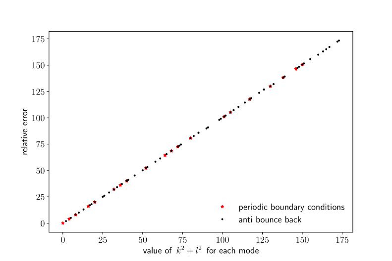
Figure 6: Relative error $\,{{\Gamma_{\rm computed}}\over{\Gamma_{\rm exact}}}-1\,$ (multiplied by $10^{4}$) as a function of the index $\,k^{2}+\ell^{2}\,$ of the modes for the Laplace equation in a square.

5)  Extended anti bounce back for general boundaries

The argument summarized in the previous section for bounce back and anti bounce back conditions can be extended to consider a boundary at an arbitrary distance $\,\eta\,\Delta x\,$ ($0<\eta<1$) from the last fluid point. It is completely described for bounce back in Bouzidi et al. [4]. Assume that the boundary is on the left for a given space direction $\,e_{j}\,$ directed towards in interior of the computational domain. The boundary node $\,x\,$ is located inside the fluid and the node $\,x+\Delta x\,$ on its right is also inside the fluid. But the node $\,x-\Delta x\,$ is not a fluid node. The outgoing particles $\,f^{*}_{j}(x)\,$ and $\,f^{*}_{j}(x+\Delta x)\,$ are known at time $\,t\,$ after the relaxation step. The incoming particle $\,f^{*}_{\ell}(x-\Delta x)\,$ for the opposite direction $\,-v_{j}\,$ ($v_{j}+v_{\ell}=0$) has to be determined by the boundary condition. This question is summarized in Figure 7.

 

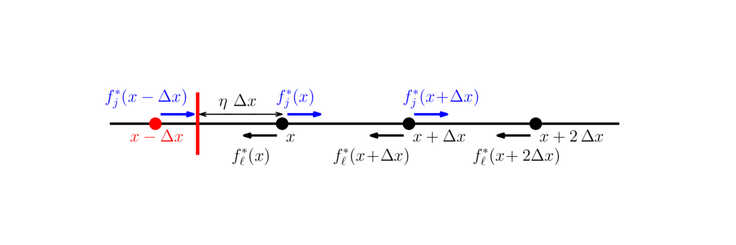
Figure 7: Boundary conditions when the boundary is not in the middle of two mesh vertices

Assuming a linear variation of the macroscopic properties of the flow, one gets (see the original derivation in [4]) extended bounce back to impose the velocity in the fluid case:

(25) $$f^{*}_{j}(x-\Delta x)=\left\{\begin{array}[]{l}\displaystyle 2\,\eta\,f^{*}_{\ell}(x)+(1-2\,\eta)\,f^{*}_{\ell}(x+\Delta x)+\xi_{j}\qquad{\rm for}\,\eta\leq{1\over 2}\\ \displaystyle\frac{1}{2\,\eta}\,f^{*}_{\ell}(x)+\Big{(}1-\frac{1}{2\,\eta}\Big{)}\,f^{*}_{j}(x)+{{\xi_{j}}\over{2\,\eta}}\,\qquad\qquad{\rm for}\,\eta\geq{1\over 2}\end{array}\right.\vspace*{-7pt}$$

or extended anti bounce back (to impose the density in the fluid case):

(26) $$f^{*}_{j}(x-\Delta x)=\left\{\begin{array}[]{l}\displaystyle-2\,\eta\,f^{*}_{\ell}(x)-(1-2\,\eta)\,f^{*}_{\ell}(x+\Delta x)+\xi_{j}\qquad{\rm for}\,\eta\leq{1\over 2}\\ \displaystyle-\frac{1}{2\,\eta}\,f^{*}_{\ell}(x)+\Big{(}1-\frac{1}{2\,\eta}\Big{)}\,f^{*}_{j}(x)+{{\xi_{j}}\over{2\,\eta}}\,\qquad\qquad{\rm for}\,\eta\geq{1\over 2}\,.\end{array}\right.\vspace*{-7pt}$$

The interpolation is done before the propagation if $\,\eta\leq{1\over 2}\,$ and after if $\,\eta\geq{1\over 2}$.

$\bullet$  Similar expressions have been written in [4] for extended bounce back assuming a parabolic variation of the velocity field

(27) $$f^{*}_{j}(x-\Delta x)=\left\{\begin{array}[]{l}\displaystyle\eta\,(1+2\,\eta)\,f^{*}_{\ell}(x)+(1-4\,\eta^{2})\,f^{*}_{\ell}(x+\Delta x)\\ \displaystyle\qquad\qquad\qquad-\eta\,(1-2\,\eta)\,f^{*}_{\ell}(x+2\,\Delta x)+\xi_{j}\qquad{\rm for}\,\eta\leq{1\over 2}\\ \displaystyle\frac{1}{\eta\,(1+2\,\eta)}\,\Big{(}f^{*}_{\ell}(x)+\xi_{j}\Big{)}+\Big{(}2-{{1}\over{\eta}}\Big{)}\,f^{*}_{j}(x)\\ \vspace{-4 mm}\displaystyle\\ \displaystyle\qquad\qquad\qquad+{{1-2\,\eta}\over{1+2\,\eta}}\,f^{*}_{j}(x+\Delta x)\,\qquad\qquad\qquad{\rm for}\,\eta\geq{1\over 2}\,.\end{array}\right.\vspace*{-7pt}$$

Similar changes in the signs as above define the extended for anti bounce back

(28) $$f^{*}_{j}(x-\Delta x)=\left\{\begin{array}[]{l}\displaystyle-\eta\,(1+2\,\eta)\,f^{*}_{\ell}(x)-(1-4\,\eta^{2})\,f^{*}_{\ell}(x+\Delta x)\\ \displaystyle\qquad\qquad\qquad+\eta\,(1-2\,\eta)\,f^{*}_{\ell}(x+2\,\Delta x)+\xi_{j}\qquad{\rm for}\,\eta\leq{1\over 2}\\ \displaystyle\frac{1}{\eta\,(1+2\,\eta)}\,\Big{(}-f^{*}_{\ell}(x)+\xi_{j}\Big{)}+\Big{(}2-{{1}\over{\eta}}\Big{)}\,f^{*}_{j}(x)\\ \vspace{-4 mm}\displaystyle\\ \displaystyle\qquad\qquad\qquad+{{1-2\,\eta}\over{1+2\,\eta}}\,f^{*}_{j}(x+\Delta x)\,\qquad\qquad\qquad{\rm for}\,\eta\geq{1\over 2}\,.\end{array}\right.\vspace*{-7pt}$$

$\bullet$  Application with the heat equation

The above anti bounce back boundary condition has been used in our previous contribution [13] in the context of the heat equation. Numerical experiments are presented in this contribution. Figures 3 and 4 with D2Q5 scheme for thermics inside a circle, and Figures 6 to 9 for D3Q7 lattice Boltzmann scheme for thermics in a three-dimensional ball. The Dirichlet boundary condition is simply implemented with an extended anti bounce back scheme.

$\bullet$  Applications with linear acoustics.

For linear acoustics, we have used in [14] the time dependent extended anti bounce back (28) to enforce a given harmonic pressure on the boundary of a disc (see the Figures 1 to 3 of this reference). No particular difficulty was reported with this treatment of the time dependent pressure boundary condition.

In this contribution, we have determined the discrete eigenmodes of the lattice Boltzmann scheme

(29) $$f_{j}(x,t+\Delta t)\,\equiv\,\exp(\Gamma\,\Delta t)\,\,f_{j}(x,t)\vspace*{-7pt}$$

for internal or boundary nodes. For a linear fluid problem, we have determined the eigenmodes (29) with the homogeneous ($\xi_{j}\equiv 0$) anti bounce back scheme (28) at the boundary. We have used the following values of relaxation parameters:

(30) $$s_{e}=1.30\,,\quad s_{x}={{1}\over{{{\sqrt{3}}\over{6}}+{1\over 2}}}\,,\quad s_{q}={{1}\over{{{\sqrt{3}}\over{3}}+{1\over 2}}}\,,\quad s_{d}=1.30\,.\vspace*{-7pt}$$

The first mode is depicted in Figures 8 and 9. An other mode is presented in Figure 10. We have no definitive interpretation of the extended bounce back and anti bounce back boundary condition (25) to (28) in terms of partial differential equations. This question is still an open problem at our knowledge. Nevertheless, some modes are clearly associated to Bessel functions. These modes are invariant by rotation as evident from these figures that include data for all points located in the circle. Recall that this is mainly due to the good choice of the quartic parameters (30) as presented in [14].

Figure 8: Linear fluid problem in a disc. Density profile as a function of the radius for the first eigenmode ($\Gamma=-0.03983758+0.00019317\,\,i\,$ in unit $\,1/\Delta t$) with homogeneous anti bounce back boundary condition for a disc with a radius $\,R=34.85$.

Figure 9: Linear fluid problem in a disc. Radial velocity profile as a function of the radius for the first eigenmode ($\Gamma=-0.03983758+0.00019317\,\,i\,$ in unit $\,1/\Delta t$) with homogeneous anti bounce back boundary condition for a disc with a radius $\,R=34.85$. A small discrepancy due to treatment of the boundary condition is visible. The tangential velocity is negligible.

Figure 10: Eigenmode $\Gamma=-1.590\,$ in unit $\,1/\Delta t\,$ for a linear fluid problem in a disc with homogeneous anti bounce back boundary condition for a disc of radius $\,R=44.2$. Tangential velocity profile as a function of the radius. The density and radial velocity are negligible for this mode.

6)  Analysis of anti bounce back for the linear fluid problem

The anti bounce back boundary condition for the fluid problem is very close to the framework presented in Section 4 for the scalar case. The boundary iteration still follows a scheme of the form (16). The collision matrix $\,C\,$ is no longer given by the relation (9), but by (13). The matrices $\,U\,$ and $\,T\,$ characterize the locus of the boundary and the anti bounce back boundary condition. They are still given by the relations (17) and (18) respectively. The matrix $\,K\,$ defined in (19) has a new expression:

(31) $$K=\left(\begin{array}[]{ccccccccc}\!\!\!\!{{1}\over{6}}(4+\alpha s_{e})&\!\!\!\!\!\!\!\!0&\!\!\!\!0&\!\!\!\!{{1}\over{6\lambda^{2}}}(1-s_{e})&\!\!\!\!{{1}\over{2\lambda^{2}}}(s_{x}-1)&\!\!\!\!\!\!\!0&\!\!\!\!0&\!\!\!\!0&\!\!\!\!0\!\!\!\!\\ \!\!\!\!0&\!\!\!\!\!\!\!\!0&\!\!\!\!0&\!\!\!\!0&\!\!\!\!0&\!\!\!\!\!\!\!{{1}\over{\lambda}}(1-s_{x})&\!\!\!\!0&\!\!\!\!0&\!\!\!\!0\!\!\!\!\\ \!\!\!\!{{\lambda}\over{6}}(4+\alpha s_{e})&\!\!\!\!\!\!\!\!0&\!\!\!\!0&\!\!\!\!{{1}\over{6\lambda}}(1-s_{e})&\!\!\!\!{{1}\over{2\,\lambda}}(s_{x}-1)&\!\!\!\!\!\!\!0&\!\!\!\!0&\!\!\!\!0&\!\!\!\!0\!\!\!\!\\ \!\!\!\!{{\lambda^{2}}\over{6}}(4-3\alpha s_{e}+2\beta s_{d})&\!\!\!\!\!\!\!\!0&\!\!\!\!0&\!\!\!\!{{1}\over{2}}(s_{e}+1)&\!\!\!\!{{1}\over{2}}(1-s_{x})&\!\!\!\!\!\!\!0&\!\!\!\!0&\!\!\!\!0&\!\!\!\!{{1}\over{3\lambda^{2}}}(1-s_{d})\!\!\!\!\\ \vspace{-.5cm}\hfil\\ \!\!\!\!{{\lambda^{2}}\over{18}}(-4+\alpha s_{e}+2\beta s_{d})&\!\!\!\!\!\!\!\!0&\!\!\!\!0&\!\!\!\!{{1}\over{18}}(1-s_{e})&\!\!\!\!{{1}\over{2}}(1+s_{x})&\!\!\!\!\!\!\!0&\!\!\!\!0&\!\!\!\!0&\!\!\!\!{{1}\over{9\lambda^{2}}}(1-s_{d})\!\!\!\!\\ \!\!\!\!0&\!\!\!\!\!\!\!\!0&\!\!\!\!0&\!\!\!\!0&\!\!\!\!0&\!\!\!\!\!\!\!1&\!\!\!\!0&\!\!\!\!0&\!\!\!\!0\!\!\!\!\\ \!\!\!\!0&\!\!\!\!\!\!\!\!\lambda^{2}s_{q}&\!\!\!\!0&\!\!\!\!0&\!\!\!\!0&\!\!\!\!\!\!\!\lambda(1-s_{x})&\!\!\!\!s_{q}&\!\!\!\!0&\!\!\!\!0\!\!\!\!\\ \!\!\!\!{{\lambda^{3}}\over{3}}(\alpha s_{e}+\beta s_{d})&\!\!\!\!\!\!\!\!0&\!\!\!\!\lambda^{2}s_{q}&\!\!\!\!{{\lambda}\over{3}}(1-s_{e})&\!\!\!\!\!\!\!\!\!\!\!\!\lambda(1-s_{x})&\!\!\!\!\!\!\!0&\!\!\!\!0&\!\!\!\!s_{q}&\!\!\!\!{{1}\over{3\lambda}}(1-s_{d})\!\!\!\!\\ \vspace{-.5cm}\hfil\\ \!\!\!\!{{\lambda^{4}}\over{3}}(\alpha s_{e}-2\beta s_{d})&\!\!\!\!\!\!\!\!0&\!\!\!\!0&\!\!\!\!{{\lambda^{2}}\over{3}}(1-s_{e})&\!\!\!\!\lambda^{2}(1-s_{x})&\!\!\!\!\!\!\!0&\!\!\!\!0&\!\!\!\!0&\!\!\!\!{{1}\over{3}}(1+2s_{d})\!\!\!\!\end{array}\right)\!.\vspace*{-7pt}$$

$\bullet$  The matrix $\,K\,$ presented in (31) is singular. The associated kernel is of dimension 2. It is generated by the following two vectors $\,\kappa_{x}\,$ and $\,\kappa_{y}\,$ in the space of moments:

(32) $$\kappa_{x}=\big{(}0,\,1,\,0,\,0,\,0,\,0,\,-\lambda^{2},\,0,\,0\big{)}^{\rm t}\,,\,\,\kappa_{y}=\big{(}0,\,0,\,1,\,0,\,0,\,0,\,0,\,-\lambda^{2},\,0\big{)}^{\rm t}\,.\vspace*{-7pt}$$

This means first that when solving a generic linear system of the type

(33) $$K\,m=g\equiv\big{(}g_{\rho},\,g_{jx},\,g_{jy},\,g_{\varepsilon},\,g_{\varphi x},\,g_{\varphi y},\,g_{qx},\,g_{qx},\,g_{h}\big{)}^{\rm t}\,,\vspace*{-7pt}$$

two compatibility relations have to be satisfied by the right hand side $\,g$:

(34) $$\lambda\,g_{\rho}-g_{jy}=0\,,\,\,\lambda\,g_{jx}+(s_{x}-1)\,g_{\varphi y}=0\,.\vspace*{-7pt}$$

Secondly, it is always possible to add to any solution of the model system (33) any combination of the type $\,j_{x}\,\kappa_{x}+j_{y}\,\kappa_{y}$. In other terms, two components $\,j_{x}\,$ and $\,j_{y}\,$ of momentum remain undetermined by the anti bounce back boundary condition. They have to be evaluated in practice by the interaction with the other vertices through the numerical scheme.

$\bullet$  Following the procedure presented previously for the thermal case, we can try to solve the boundary condition (20) at various orders. At order zero, no relevant information is given by the compatibility conditions (34). Then the solution $\,m_{0}\,$ at order zero depends on two parameters identified as the momentum $\,(j_{x},\,j_{y})\,$ in the first cell. With a given pressure $\,p_{0}\,$ or a given density $\,\rho_{0}\equiv{{p_{0}}\over{c_{0}^{2}}}\,$ on the boundary, we have

(35) $$m_{0}=\left(\rho_{0},\,j_{x},\,j_{y},\,\alpha\,\lambda^{2}\,\rho_{0},\,0,\,0,\,-\lambda^{2}\,j_{x},\,-\lambda^{2}\,j_{y},\,\beta\,\,\lambda^{4}\rho_{0}\right)^{\rm t}\,.\vspace*{-7pt}$$

At order one, the first compatibility relation is a linear combination of the first order equivalent partial differential equations. The other compatibility relation gives a non trivial differential condition on the boundary :

(36) $$\partial_{x}J_{y}+\partial_{y}J_{x}=0\,.\vspace*{-7pt}$$

The anti bounce back induces a hidden additional boundary condition. Observe that the differential condition (36) is not satisfied for a Poiseuille flow. Nevertheless, if this relation is satisfied, it is possible to expand the resulting density in the first cell:

(37) $$\rho\Big{(}x_{1},{{\Delta x}\over{2}}\Big{)}=\rho_{0}\big{(}x_{1}\big{)}+{{1}\over{2}}\,\Delta x\,\,\partial_{y}\rho(x_{1})+\Delta t\,\big{(}a_{jx}\,\,\partial_{x}J_{x}+a_{jy}\,\,\partial_{y}J_{y}\big{)}+{\rm O}(\Delta x^{2})\,.\vspace*{-7pt}$$

with

$$\left\{\begin{array}[]{l}\displaystyle a_{jx}={{1}\over{8\,(s_{e}\,s_{x}+s_{e}\,s_{d}+s_{x}\,s_{d})+2\,(s_{e}\,s_{x}+2\,s_{e}\,s_{d})\,\alpha+2\,(s_{e}\,s_{d}-s_{x}\,s_{d})\,\beta}}\,\Big{(}6\,s_{e}\,s_{x}+5\,s_{e}\,s_{d}\\ \displaystyle\qquad\qquad+\,7\,s_{x}\,s_{d}-6\,s_{e}+2\,s_{x}-8\,s_{d}+2\,(s_{e}\,s_{x}+2\,s_{e}\,s_{d}-s_{x}-2\,s_{d})\,\alpha\\ \displaystyle\qquad\qquad+2\,(s_{e}\,s_{d}-s_{x}\,s_{d}-s_{e}+s_{x})\,\beta\Big{)}\\ \vspace{-4 mm}\displaystyle\\ \displaystyle a_{jy}={{1}\over{8\,(s_{e}\,s_{x}+s_{e}\,s_{d}+s_{x}\,s_{d})+2\,(s_{e}\,s_{x}+2\,s_{e}\,s_{d})\,\alpha+2\,(s_{e}\,s_{d}-s_{x}\,s_{d})\,\beta}}\,\Big{(}2\,s_{e}\,s_{x}+5\,s_{e}\,s_{d}\\ \displaystyle\qquad\qquad-\,s_{x}\,s_{d}+2\,s_{e}+2\,s_{x}+8\,s_{d}+2\,(s_{e}\,s_{x}+2\,s_{e}\,s_{d}-s_{x}-2\,s_{d})\,\alpha\\ \displaystyle\qquad\qquad+2\,(s_{e}\,s_{d}-s_{x}\,s_{d}-s_{e}+s_{x})\,\beta\Big{)}\,.\end{array}\right.\vspace*{-6pt}$$

This result indicates that the anti bounce back boundary condition gives not satisfactory results for the field near the boundary. The extra term $\,a_{jx}\,\,\partial_{x}J_{x}+a_{jy}\,\,\partial_{y}J_{y}\,$ in the relation (37) is a discrepancy if we compare this relation with a common Taylor expansion of the density in the normal direction as found in the scalar case (24). The relations (36) and (37) put in evidence quantitatively various defects of the anti bounce back boundary condition as proposed at the relations (14).

$\bullet$  Numerical experiments for a linear Poiseuille flow.

We have considered a two-dimensional vertical channel with wall boundaries at the left and at the right. At the bottom of the channel a given $\,+P_{0}\,$ pressure is imposed through anti bounce back and $\,-P_{0}\,$ is imposed at the top (see Figure 11).

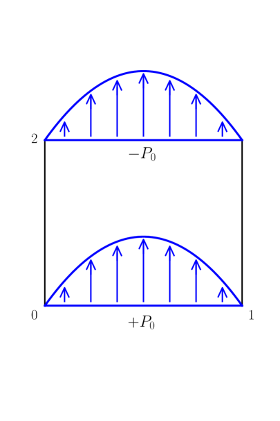
Figure 11: Linear vertical Poiseuille flow. The solid boundaries are at the left and at the right. A given pressure of $\,P_{0}=0.001\,$ and $\,-P_{0}\,$ are given at the bottom and the top of the channel. A parabolic profile is generated by the pressure gradient.

We have emphasized in Figures 12, 13, 14 and 15 the results for three meshes with $20\times 40$, $40\times 80\,$ and $\,80\times 160\,$ cells. In Figure 12, the field is represented in the first two layers near the inflow boundary. Due to the classical Taylor expansion [26]

$$\varphi_{y}=-{{\lambda\,\Delta x}\over{3\,s_{x}}}\,\big{(}\partial_{x}J_{y}+\partial_{y}J_{x}\big{)}+{\rm O}(\Delta x^{2})\,,\vspace*{-6pt}$$

this field is an excellent indicator of the treatment of the hidden boundary condition (36). The Figure 12 confirms that for the first cell, the hidden condition is effectively taken into account, except may be in the corners.

In consequence, the Poiseuille flow cannot be correctly satisfied near the fluid boundary. An important error of 18.2% for the pressure in the first cell is observed for the three meshes (see Fig. 13). Nevertheless, if we fit these pressure results by linear curves taking only half the number of points in the middle of the channel, this error is reduced to 6.5% (see Fig. 13). The tangential velocity is supposed to be identically null in all the channel. In the middle, the maximal tangential velocity is always less than 0.01% of the maximum normal velocity. But in the first cells (Fig. 14), the discrepancies are important and can reach 17% of the maximal velocity.

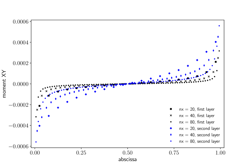
Figure 12: Anti bounce back boundary condition for linear Poiseuille flow. Moment field $\,\varphi_{y}$ in the first layers of the boundary. The hidden boundary condition $\,\partial_{x}J_{y}+\partial_{y}J_{x}=0\,$ enforces the constraint $\,XY\equiv\varphi_{y}=0$.

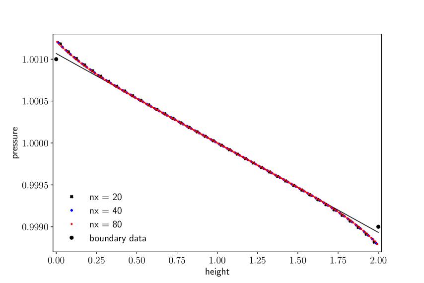
Figure 13: Anti bounce back boundary condition for linear Poiseuille flow. Pressure field in the middle of the channel (after a simple interpolation due to an even number of meshes) for three meshes with $20\times 40$, $40\times 80\,$ and $\,80\times 160\,$ cells. A substantial error does not vanish as the mesh size tends to zero.

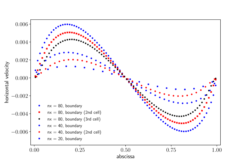
Figure 14: Anti bounce back boundary condition for linear Poiseuille flow. Horizontal velocity field for three meshes. The maximum value is around 17% of the vertical velocity.

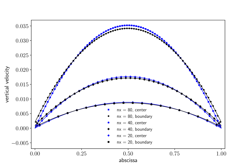
Figure 15: Anti bounce back boundary condition for linear Poiseuille flow. Vertical velocity field for three meshes. The parabolic profile is not completely recovered, in particular in the cells near the fluid boundary.

In Figure 15, the axial velocity is presented for the three meshes. We keep the same value of $\,s_{x}\,$ and in consequence the kinematic viscosity of the fluid [12, 26]

$$\nu={{\lambda}\over{3}}\,\Delta x\,\Big{(}{{1}\over{s_{x}}}-{1\over 2}\Big{)}\,\vspace*{-6pt}$$

is reduced at each mesh refinement by a factor of 2 and the normal velocity is multiplied in the same proportions. We have fitted with least squares the vertical velocity by a parabola in the middle of the channel and in the first layer (see Figure 15). The null velocity along this fitted parabola defines a numerical boundary that is compared to its true geometric location. The results are presented in Table 3. In the center of the channel, we obtain a typical error of $\,10^{-3}\,$ between the numerical and geometrical boundaries, measured in cell units: the axial velocity is of very good quality in the center of the channel. In the first cell, the gap between numerical and physical boundaries represents a notable fraction of one unit cell (see Table 3).

mesh $20\times 40$ $40\times 80$ $80\times 160$ center $5.29\,10^{-3}$ $3.98\,10^{-3}$ $4.61\,10^{-3}$ bottom $0.261$ $0.582$ $1.26$

Table 3: Anti bounce back boundary condition for linear Poiseuille flow. Distance between the numerical position of the boundary from its theoretical location.

7)  Mixing bounce back and anti bounce back boundary conditions

In order to overcome the difficulties with the anti bounce back boundary condition for the fluid problem, we have adapted a mixing of bounce back and anti bounce back first proposed in [15] for the thermal Navier-Stokes equations. We suppose that all the fluid information, id est density and momentum, is given on the boundary. We force this relation by taking bounce back boundary condition for the particles coming from the left and from the right: $\,f_{5}^{\rm eq}-f_{7}^{\rm eq}={{1}\over{6\,\lambda}}\,(J_{x}+J_{y})\,$ and $\,f_{6}^{\rm eq}-f_{8}^{\rm eq}={{1}\over{6\,\lambda}}\,(-J_{x}+J_{y})$. We keep the anti bounce back $\,f_{2}^{\rm eq}+f_{4}^{\rm eq}={{4-\alpha-2\,\beta}\over{18}}\,\rho\,$ for the particles coming from the bottom, as illustrated in Figure 16.

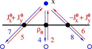
Figure 16: Mixed bounce back and anti bounce back boundary condition to enforce density and momentum values on the boundary.

Finally, if density $\,\rho_{0}\,$ and the two components $\,J_{x}^{0}\,$ and $\,J_{y}^{0}\,$ of the velocity are supposed given on the boundary, the mixed bounce back and anti bounce back boundary condition can be written as:

(38) $$\left\{\begin{array}[]{l}\displaystyle f_{5}(x,\,t+\Delta t)=f^{*}_{7}(x,\,t)\,+\,{{1}\over{6\,\lambda}}\,\big{(}J_{x}^{0}+J_{y}^{0}\big{)}\Big{(}x_{1}-{{\Delta x}\over{2}},\,t\Big{)}\,,\\ \vspace{-4 mm}\\ \displaystyle f_{2}(x,\,t+\Delta t)=-f^{*}_{4}(x,\,t)\,+\,{{4-\alpha-2\,\beta}\over{18}}\,\rho_{0}\big{(}x_{1},\,t\big{)}\,,\\ \vspace{-4 mm}\\ \displaystyle\displaystyle f_{6}(x,\,t+\Delta t)=f^{*}_{8}(x,\,t)\,+\,{{1}\over{6\,\lambda}}\,\big{(}-J_{x}^{0}+J_{y}^{0}\big{)}\Big{(}x_{1}+{{\Delta x}\over{2}},\,t\Big{)}\,.\end{array}\right.\vspace*{-7pt}$$

$\bullet$  The analysis of the discrete mixed condition (38) follows the methodology presented above. The boundary iteration still follows the general framework (16). The matrices $\,U\,$ and $\,T\,$ characterize the locus of the boundary and the mixed bounce back and anti bounce back boundary condition. The matrix $\,U\,$ is still given by (17). On the contrary, the interaction matrix $\,T\,$ is no longer given by the expression (18), but by the relation

(39) $$T=\left(\begin{array}[]{ccccccccc}0&0&0&0&0&0&0&0&0\\ 0&0&0&0&0&0&0&0&0\\ 0&0&0&0&\!-1&0&0&0&0\\ 0&0&0&0&0&0&0&0&0\\ 0&0&0&0&0&0&0&0&0\\ 0&0&0&0&0&0&0&\!+1&0\\ 0&0&0&0&0&0&0&0&\!+1\\ 0&0&0&0&0&0&0&0&0\\ 0&0&0&0&0&0&0&0&0\end{array}\right)\,.\vspace*{-7pt}$$

The matrix $\,K\,$ introduced in (19) takes the form:

(40) $$K=\left(\begin{array}[]{ccccccccc}\!\!\!\!{{4-\alpha s_{e}-2\beta s_{d}}\over{18}}&\!\!\!\!\!\!\!0&\!\!\!\!\!\!\!\!{{2-s_{q}}\over{3\lambda}}&\!\!\!\!\!{{s_{e}-1}\over{18\lambda^{2}}}&\!\!\!\!{{s_{x}-1}\over{2\lambda^{2}}}&\!\!\!\!\!\!\!0&\!\!\!\!\!\!\!0&\!\!\!\!{{1-s_{q}}\over{3\,\lambda^{3}}}&\!\!\!\!{{s_{d}-1}\over{9\lambda^{4}}}\\ \!\!\!\!0&\!\!\!\!\!\!\!{{2-s_{q}}\over{3}}&\!\!\!\!\!\!\!\!0&\!\!\!\!\!0&\!\!\!\!0&\!\!\!\!\!\!\!0&\!\!\!\!{{1-s_{q}}\over{3\lambda^{2}}}&\!\!\!\!0&\!\!\!\!0\\ \!\!\!\!{{\lambda(4-\alpha s_{e}-2\beta s_{d})}\over{18}}&\!\!\!\!\!\!\!0&\!\!\!\!\!\!\!\!{{2-s_{q}}\over{3}}&\!\!\!\!\!{{s_{e}-1}\over{18\lambda}}&\!\!\!\!{{s_{x}-1}\over{2\lambda}}&\!\!\!\!\!\!\!0&\!\!\!\!0&\!\!\!\!{{1-s_{q}}\over{3\lambda^{2}}}&\!\!\!\!{{s_{d}-1}\over{9\lambda^{3}}}\\ \!\!\!\!{{\lambda^{2}(-4-17\alpha s_{e}+2\beta s_{d})}\over{18}}&\!\!\!\!\!\!\!0&\!\!\!\!\!\!\!\!{{\lambda(4-2s_{q})}\over{3}}&\!\!\!\!\!{{1+17s_{e}}\over{18}}&\!\!\!\!{{1-s_{x}}\over{2}}&\!\!\!\!\!\!\!0&\!\!\!\!0&\!\!\!\!{{2(1-s_{q})}\over{3\lambda}}&\!\!\!\!{{1-s_{d}}\over{3\lambda^{2}}}\\ \!\!\!\!{{\lambda^{2}(-4+\alpha s_{e}+2\beta s_{d})}\over{18}}&\!\!\!\!\!\!\!0&\!\!\!\!\!\!\!\!0&\!\!\!\!\!{{1-s_{e}}\over{18}}&\!\!\!\!{{1+s_{x}}\over{2}}&\!\!\!\!\!\!\!0&\!\!\!\!0&\!\!\!\!0&\!\!\!\!{{1-s_{d}}\over{9\lambda^{2}}}\\ \!\!\!\!0&\!\!\!\!\!\!\!\!{{\lambda(2-s_{q})}\over{3}}&\!\!\!\!\!\!\!\!0&\!\!\!\!\!0&\!\!\!\!0&\!\!\!\!\!\!\!s_{x}&\!\!\!\!{{1-s_{q}}\over{3\lambda}}&\!\!\!\!0&\!\!\!\!0\\ \!\!\!\!0&\!\!\!\!\!\!\!{{2\lambda^{2}(1+s_{q})}\over 3}&\!\!\!\!\!\!\!\!0&\!\!\!\!\!0&\!\!\!\!0&\!\!\!\!\!\!\!0&\!\!\!\!{{1+2s_{q}}\over 3}&\!\!\!\!0&\!\!\!\!0\\ \!\!\!\!{{\lambda^{3}(-4+\alpha s_{e}+2\beta s_{d})}\over{9}}&\!\!\!\!\!\!\!0&\!\!\!\!\!\!\!\!{{2\lambda^{2}(1+s_{q})}\over 3}&\!\!\!\!\!{{\lambda(1-s_{e})}\over{9}}&\!\!\!\!\lambda(1\!\!-\!\!s_{x}\!)&\!\!\!\!\!\!\!0&\!\!\!\!0&\!\!\!\!{{1+2s_{q}}\over 3}&\!\!\!\!{{2(1-s_{d})}\over{9\lambda}}\\ \!\!\!\!{{\lambda^{4}(-4+\alpha s_{e}-7\beta s_{d})}\over{9}}&\!\!\!\!\!\!\!0&\!\!\!\!\!\!\!\!{{\lambda^{3}(2-s_{q})}\over{3}}&\!\!\!\!\!{{\lambda^{2}(1-s_{e})}\over{3}}&\!\!\!\!\lambda^{2}(1\!\!-\!\!s_{x}\!)&\!\!\!\!0&\!\!\!\!0&\!\!\!\!\!\!\!{{\lambda(1-s_{q})}\over{3}}&\!\!\!\!{{2+7s_{d}}\over{9}}\end{array}\right)\,.\vspace*{-7pt}$$

The matrix defined in (40) is singular. Its kernel is of dimension 1. It is generated by the following vector $\,\kappa$:

$$\kappa=\begin{pmatrix}\displaystyle{{(3\,s_{e}\,s_{d}+2\,s_{e}\,s_{x}+s_{d}\,s_{x})\,s_{q}}\over{\lambda\,s_{d}\,s_{e}\,s_{x}\,(\alpha+2\,\beta-4)}}\\ \vspace{-4 mm}\\ \displaystyle 0\\ 1\\ \displaystyle{{\lambda\,(3\,\alpha\,s_{e}\,s_{d}+2\,\alpha\,s_{e}\,s_{x}-2\,\beta\,s_{d}\,s_{x}+4\,s_{d}\,s_{x})\,s_{q}}\over{s_{d}\,s_{e}\,s_{x}\,(\alpha+2\,\beta-4)}}\\ \vspace{-4 mm}\\ \displaystyle{{\lambda\,s_{q}}\over{3\,s_{x}}}\\ 0\\ 0\\ \displaystyle-2\,\lambda^{2}\\ \vspace{-4 mm}\\ \displaystyle-\lambda^{3}\,{{\alpha\,s_{e}\,s_{x}-3\,\beta\,s_{e}\,s_{d}-\beta\,s_{d}\,s_{x}-4\,s_{e}\,s_{x})\,s_{q}}\over{s_{d}\,s_{e}\,s_{x}\,(\alpha+2\,\beta-4)}}\\ \end{pmatrix}\,.\vspace*{-6pt}$$

We did not find any simple physical interpretation of the kernel $\,\mathbb{R}\kappa\,$ of the matrix $\,K\,$ defined by (40) in this case. When solving the generic linear system (33), the right hand side $\,g\,$ must satisfy

$$\lambda\,g_{\rho}-g_{jy}=0\,.\vspace*{-6pt}$$

Moreover, the solution is defined up to a multiple of the vector $\,\kappa\,$ presented above.

$\bullet$  At order zero, the compatibility condition does not give any relevant information. If we suppose that the component of $\,m_{0}\,$ along the eigenvector $\,\kappa\,$ is reduced to zero, we have for a given density $\,\rho_{0}\,$ and a given momentum $\,(J_{x}^{0},\,J_{y}^{0})\,$ on the boundary:

$$m_{0}=\left(\rho_{0},\,J_{x}^{0},\,J_{y}^{0},\,\alpha\,\lambda^{2}\,\rho_{0},\,0,\,0,\,-\lambda^{2}\,J_{x}^{0},\,-\lambda^{2}\,J_{y}^{0},\,\beta\,\,\lambda^{4}\rho_{0}\right)^{\rm t}\,.\vspace*{-6pt}$$

At order one the compatibility relations is a linear combination of the first order equivalent partial differential equations and no constraint is added by this relation. The resulting moments in the first cell $\,x\equiv\big{(}x_{1},\,{{\Delta x}\over{2}}\big{)}\,$ at first order can be expressed after some formal calculus:

(41) $$\left\{\begin{array}[]{l}\displaystyle\rho\Big{(}x_{1},\,{{\Delta x}\over{2}}\Big{)}=\rho_{0}\big{(}x_{1}\big{)}+{{1}\over{2}}\,\Delta x\,\partial_{y}\rho\big{(}x_{1},\,0\big{)}+{{\Delta x}\over{s_{x}\,s_{e}\,s_{d}\,(\alpha+2\,\beta-4)}}\,\Big{(}a_{\rho}\,\,\partial_{y}\rho\big{(}x_{1},\,0\big{)}\\ \vspace{-4 mm}\\ \displaystyle\qquad\qquad\qquad\qquad\qquad+\,b_{\rho}\,\,\partial_{x}J_{x}\big{(}x_{1},\,0\big{)}+c_{\rho}\,\,\partial_{y}J_{y}\big{(}x_{1},\,0\big{)}\Big{)}+{\rm O}(\Delta x^{2})\,,\\ \vspace{-4 mm}\\ \displaystyle j_{x}\Big{(}x_{1},\,{{\Delta x}\over{2}}\Big{)}=J_{x}^{0}\big{(}x_{1}\big{)}+{1\over 2}\,\Delta x\,\,\partial_{y}J_{x}\big{(}x_{1},\,0\big{)}+{\rm O}(\Delta x^{2})\,,\end{array}\right.\vspace*{-7pt}$$

with

(42) $$\left\{\begin{array}[]{l}\displaystyle a_{\rho}={1\over 6}\,\Big{(}-4\,(2\,s_{e}\,s_{x}+3\,s_{e}\,s_{d}+s_{x}\,s_{d})\\ \vspace{-4 mm}\\ \displaystyle\qquad\qquad\qquad+\,(2\,s_{e}\,s_{x}\,s_{q}+3\,s_{e}\,s_{q}\,s_{d}+s_{x}\,s_{q}\,s_{d}-6\,s_{e}\,s_{x}-9\,s_{e}\,s_{d}-3\,s_{x}\,s_{d})\,\alpha\\ \vspace{-4 mm}\\ \displaystyle\qquad\qquad\qquad+\,(2\,s_{e}\,s_{x}\,s_{q}+3\,s_{e}\,s_{q}\,s_{d}+s_{x}\,s_{q}\,s_{d}-4\,s_{e}\,s_{x}-6\,s_{e}\,s_{d}-2\,s_{x}\,s_{d})\,\beta\Big{)}\,,\\ \vspace{-4 mm}\\ \displaystyle b_{\rho}=2\,s_{e}\,(3\,s_{d}-2\,s_{x}\,s_{d}-s_{x})+s_{x}\,s_{d}\,(s_{e}-1)\,\alpha+2\,s_{e}\,s_{x}\,(s_{d}-1)\,\beta\,,\\ \vspace{-4 mm}\\ \displaystyle c_{\rho}={1\over 2}\,\Big{(}4\,s_{e}\,s_{x}\,s_{d}-2\,s_{e}\,s_{x}\,s_{q}-3\,s_{e}\,s_{q}\,s_{d}-s_{x}\,s_{q}\,s_{d}-4\,s_{e}\,s_{x}-12\,s_{e}\,s_{d}\\ \vspace{-4 mm}\\ \displaystyle\qquad\qquad\qquad+2\,s_{x}\,s_{d}\,(s_{e}-1)\,\alpha+4\,(s_{d}-1)\,s_{e}\,s_{x}\,\beta\Big{)}\end{array}\right.\vspace*{-7pt}$$

and

(43) $$j_{y}\Big{(}x_{1},\,{{\Delta x}\over{2}}\Big{)}=J_{y}^{0}\big{(}x_{1}\big{)}+{\rm O}(\Delta x^{2})\,.\vspace*{-7pt}$$

We are puzzled by this result and more work is needed. There is a true discrepancy for the density with the three terms parametrized by the coefficients $\,a_{\rho}$, $\,b_{\rho}\,$ and $\,c_{\rho}$. Moreover, no first order term $\,{1\over 2}\,\Delta x\,\partial_{y}J_{y}\,$ of a simple Taylor formula is present for the expansion (43) of the normal momentum.

8)  Giving pressure and tangential velocity on the boundary

A natural mathematical question is to know whether a given set of partial differential equations associated with a given set of boundary conditions conducts to a well posed problem in the sense of Hadamard. For example, the Poisson equation with Dirichlet or Neumann boundary conditions conducts to a well posed problem (see e.g. [19]). On the contrary for the same Laplace equations, the Cauchy problem is defined by the fact to impose the value of the unknown field and the value of the normal derivative on some part of the boundary. As well known, this Cauchy problem for the Laplace equation is not correctly posed [5, 9]. For the stationary Stokes problem

$${\rm div}u=0\,,\quad-\nu\,\Delta u+\nabla p=0\,,\vspace*{-6pt}$$

a set of correctly posed boundary conditions is based on the velocity vorticity pressure formulation [10]:

(44) $${\rm div}u=0\,,\quad\omega-{\rm curl}\,u=0\,,\quad\nu\,{\rm curl}\,\omega+\nabla p=0\,.\vspace*{-7pt}$$

Considering a variational formulation of the Stokes system (44), natural boundary conditions can be derived and we obtain the following procedure. Consider the two following decompositions $\,\Gamma_{m}\cup\Gamma_{p}\,$ and $\,\Gamma_{t}\cup\Gamma_{\theta}\,$ of the boundary $\,\partial\Omega$:

$$\left\{\begin{array}[]{l}\displaystyle\partial\Omega=\Gamma_{m}\cup\Gamma_{p}\quad{\rm with}\,\,{\rm meas}\,\big{(}\Gamma_{m}\cap\Gamma_{p}\big{)}=0\,,\\ \partial\Omega=\Gamma_{t}\cup\Gamma_{\theta}\quad\,\,{\rm with}\,\,{\rm meas}\,\big{(}\Gamma_{t}\cap\Gamma_{\theta}\big{)}=0\,.\end{array}\right.\vspace*{-6pt}$$

Suppose now that on one hand, the normal velocity is given on $\,\Gamma_{m}\,$ and the pressure is given on $\,\Gamma_{p}\,$ and on the other hand that the tangential velocity is given on $\,\Gamma_{t}\,$ and the tangential vorticity is imposed on $\,\Gamma_{\theta}$:

(45) $$\left\{\begin{array}[]{ll}\displaystyle u\cdot n=g_{0}\quad{\rm on}\,\,\,\Gamma_{m}\,,&p=\Pi_{0}\quad{\rm on}\,\,\,\Gamma_{p}\\ n\times u\times n=\sigma_{0}\quad{\rm on}\,\,\,\Gamma_{t}\,,&n\times\omega\times n=\theta_{0}\quad{\rm on}\,\,\,\,\Gamma_{\theta}\,.\end{array}\right.\vspace*{-7pt}$$

Then under some technical hypotheses, the Stokes problem (44) with the boundary conditions (45) admits a unique variational solution in ad hoc vectorial Sobolev spaces [11]. A first particular case is the Dirichlet problem, where both components of velocity are given (see e.g. [21]). An interesting case is the fact to give pressure and tangential velocity, as first remarked in [3]:

(46) $$p=\Pi_{0}\quad{\rm and}\quad n\times u\times n=\sigma_{0}\quad{\rm on}\,\,\,\Gamma\,.\vspace*{-7pt}$$

In the following of this section, we propose to adapt the algorithm proposed in Section 6 to the set of boundary conditions (46).

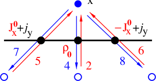
Figure 17: Mixed bounce back and anti bounce back boundary condition to enforce density and tangential velocity on the boundary.

$\bullet$  We suppose in this section that the density $\,\rho=\rho_{0}\,$ and the tangential momentum $\,J_{x}=J_{x}^{0}\,$ are given on the boundary. The momentum nodal values in the first cell are still denoted as $\,j_{x}\,$ and $\,j_{y}$. From the previous given equilibrium (12), we can write the bounce back boundary condition for diagonal edges $\,f_{5}^{\rm eq}-f_{7}^{\rm eq}={{1}\over{6\,\lambda}}\,(J_{x}^{0}+j_{y})$, $\,f_{6}^{\rm eq}-f_{8}^{\rm eq}={{1}\over{6\,\lambda}}\,(-J_{x}^{0}+j_{y})$. The anti bounce back is unchanged: $\,f_{2}^{\rm eq}+f_{4}^{\rm eq}={{4-\alpha-2\,\beta}\over{18}}\,\rho_{0}\,$ for the particles coming from the bottom, as illustrated in Figure 17. If $\,x\equiv\big{(}x_{1},\,{{\Delta x}\over{2}}\big{)}\,$ is the notation for the first fluid node, the boundary condition on pressure and tangential velocity is finally implemented in the D2Q9 algorithm with the relations

(47) $$\left\{\begin{array}[]{l}\displaystyle f_{5}(x,\,t+\Delta t)=f^{*}_{7}(x,\,t)\,+\,{{1}\over{6\,\lambda}}\,\Big{[}J_{x}^{0}\Big{(}x_{1}-{{\Delta x}\over{2}},\,t\Big{)}+j_{y}(x,\,t)\Big{]}\,,\\ \vspace{-4 mm}\\ \displaystyle f_{2}(x,\,t+\Delta t)=-f^{*}_{4}(x,\,t)\,+\,{{4-\alpha-2\,\beta}\over{18}}\,\rho_{0}\big{(}x_{1},\,t\big{)}\,,\\ \vspace{-4 mm}\\ \displaystyle\displaystyle f_{6}(x,\,t+\Delta t)=f^{*}_{8}(x,\,t)\,+\,{{1}\over{6\,\lambda}}\,\Big{[}-J_{x}^{0}\Big{(}x_{1}+{{\Delta x}\over{2}},\,t\Big{)}+j_{y}(x,\,t)\Big{]}\,.\end{array}\right.\vspace*{-7pt}$$

$\bullet$  The asymptotic analysis of the condition (47) follows the general framework (16). The matrix $\,U\,$ is still given by (17). The interaction matrix $\,T\,$ follows now the relation

(48) $$T=\left(\begin{array}[]{ccccccccc}0&0&0&0&0&0&0&0&0\\ 0&0&0&0&0&0&0&0&0\\ 0&0&0&0&\!-1&0&0&0&0\\ 0&0&0&0&0&0&0&0&0\\ 0&0&0&0&0&0&0&0&0\\ 0&0&{1\over 6}&0&\!-{1\over 6}&{1\over 6}&{1\over 6}&\!{5\over 6}&\!-{1\over 6}\\ 0&0&{1\over 6}&0&\!-{1\over 6}&{1\over 6}&{1\over 6}&\!-{1\over 6}&\!{5\over 6}\\ 0&0&0&0&0&0&0&0&0\\ 0&0&0&0&0&0&0&0&0\end{array}\right)\,.\vspace*{-7pt}$$

The matrix $\,K\,$ of (19) is now equal to

(49) $$K=\left(\begin{array}[]{ccccccccc}\!\!\!\!{{4-\alpha s_{e}-2\beta s_{d}}\over{18}}&\!\!\!\!\!\!\!0&\!\!\!\!\!\!\!\!{{1-s_{q}}\over{3\lambda}}&\!\!\!\!\!{{s_{e}-1}\over{18\lambda^{2}}}&\!\!\!\!{{s_{x}-1}\over{2\lambda^{2}}}&\!\!\!\!\!\!\!0&\!\!\!\!\!\!\!0&\!\!\!\!{{1-s_{q}}\over{3\lambda^{3}}}&\!\!\!\!{{s_{d}-1}\over{9\lambda^{4}}}\\ \!\!\!\!0&\!\!\!\!\!\!\!{{2-s_{q}}\over{3}}&\!\!\!\!\!\!\!\!0&\!\!\!\!\!0&\!\!\!\!0&\!\!\!\!\!\!\!0&\!\!\!\!{{1-s_{q}}\over{3\lambda^{2}}}&\!\!\!\!0&\!\!\!\!0\\ \!\!\!\!{{\lambda(4-\alpha s_{e}-2\beta s_{d})}\over{18}}&\!\!\!\!\!\!\!0&\!\!\!\!\!\!\!\!{{1-s_{q}}\over{3}}&\!\!\!\!\!{{s_{e}-1}\over{18\lambda}}&\!\!\!\!{{s_{x}-1}\over{2\lambda}}&\!\!\!\!\!\!\!0&\!\!\!\!0&\!\!\!\!{{1-s_{q}}\over{3\lambda^{2}}}&\!\!\!\!{{s_{d}-1}\over{9\lambda^{3}}}\\ \!\!\!\!{{\lambda^{2}(-4-17\alpha s_{e}+2\beta s_{d})}\over{18}}&\!\!\!\!\!\!\!0&\!\!\!\!\!\!\!\!{{2\lambda(1-s_{q})}\over{3}}&\!\!\!\!\!{{1+17s_{e}}\over{18}}&\!\!\!\!{{1-s_{x}}\over{2}}&\!\!\!\!\!\!\!0&\!\!\!\!0&\!\!\!\!{{2(1-s_{q})}\over{3\lambda}}&\!\!\!\!{{1-s_{d}}\over{9\lambda^{2}}}\\ \!\!\!\!{{\lambda^{2}(-4+\alpha s_{e}+2\beta s_{d})}\over{18}}&\!\!\!\!\!\!\!0&\!\!\!\!\!\!\!\!0&\!\!\!\!\!{{1-s_{e}}\over{18}}&\!\!\!\!{{1+s_{x}}\over{2}}&\!\!\!\!\!\!\!0&\!\!\!\!0&\!\!\!\!0&\!\!\!\!{{1-s_{d}}\over{9\lambda^{2}}}\\ \!\!\!\!0&\!\!\!\!\!\!\!\!{{\lambda(2-s_{q})}\over{3}}&\!\!\!\!\!\!\!\!0&\!\!\!\!\!0&\!\!\!\!0&\!\!\!\!\!\!\!s_{x}&\!\!\!\!{{1-s_{q}}\over{3\lambda}}&\!\!\!\!0&\!\!\!\!0\\ \!\!\!\!0&\!\!\!\!\!\!\!{{2\lambda^{2}(1+s_{q})}\over 3}&\!\!\!\!\!\!\!\!0&\!\!\!\!\!0&\!\!\!\!0&\!\!\!\!\!\!\!0&\!\!\!\!{{1+2s_{q}}\over 3}&\!\!\!\!0&\!\!\!\!0\\ \!\!\!\!{{\lambda^{3}(-4+\alpha s_{e}+2\beta s_{d})}\over{9}}&\!\!\!\!\!\!\!0&\!\!\!\!\!\!\!\!{{\lambda^{2}(1+2s_{q})}\over 3}&\!\!\!\!\!{{\lambda(1-s_{e})}\over{9}}&\!\!\!\!\lambda(1\!\!-\!\!s_{x}\!)&\!\!\!\!\!\!\!0&\!\!\!\!0&\!\!\!\!{{1+2s_{q}}\over 3}&\!\!\!\!{{2(1-s_{d})}\over{9\lambda}}\\ \!\!\!\!{{\lambda^{4}(-4+\alpha s_{e}-7\beta s_{d})}\over{9}}&\!\!\!\!\!\!\!0&\!\!\!\!\!\!\!\!{{\lambda^{3}(1-s_{q})}\over{3}}&\!\!\!\!\!{{\lambda^{2}(1-s_{e})}\over{3}}&\!\!\!\!\lambda^{2}(1\!\!-\!\!s_{x}\!)&\!\!\!\!0&\!\!\!\!0&\!\!\!\!\!\!\!{{\lambda(1-s_{q})}\over{3}}&\!\!\!\!{{2+7s_{d}}\over{9}}\end{array}\right)\,.\vspace*{-7pt}$$

The matrix $K$ is singular. Its kernel is of dimension 1. The null eigenvector of the matrix $\,K\,$ is exactly $\,\kappa_{y}\,$ introduced in (32):

$$\kappa_{y}=\big{(}0,\,0,\,1,\,0,\,0,\,0,\,0,\,-\lambda^{2},\,0\big{)}^{\rm t}\,.\vspace*{-6pt}$$

$\bullet$  The associated compatibility relation for solving the linear system (33) is analogous to previous ones:

(50) $$\lambda\,g_{\rho}-g_{jy}=0\,.\vspace*{-7pt}$$

From the relation (47), the right hand side

$$\xi=\xi_{0}+\Delta t\,\,\partial\xi+{\rm O}(\Delta t^{2})\,\vspace*{-6pt}$$

can be easily described:

$$\left\{\begin{array}[]{ll}\displaystyle\xi_{0}\!&=\displaystyle\,\Big{(}0\,,\,0\,,\,{1\over 18}\,(-\alpha-2\,\beta+4)\,\rho_{0}\,,\,0\,,\,0\,,\,{1\over{6\,\lambda}}\,J_{x}^{0}\,,\,-{1\over{6\,\lambda}}\,J_{x}^{0}\,,\,0\,,\,0\Big{)}^{\textrm{t}}\\ \partial\xi\!&=\displaystyle\,\Big{(}0\,,\,0\,,\,0\,,\,0\,,\,0\,,\,-{1\over{12}}\,\partial_{x}J_{x}^{0}\,,\,-{1\over{12}}\,\partial_{x}J_{x}^{0}\,,\,0\,,\,0\Big{)}^{\!\textrm{t}}\,.\end{array}\right.\vspace*{-6pt}$$

At order zero, the compatibility relation (50) does not give any condition. At first order, the compatibility relation reduces to a combination of the associated partial differential equations. In consequence, no hidden boundary condition is introduced with this mixed bounce back and anti bounce back boundary condition. As designed by the boundary conditions (47), the normal momentum $\,j_{y}\,$ is not defined on the boundary. Then all the results are defined up to a multiple $\,j_{y}\,\kappa_{y}\,$ in the kernel of the matrix $\,K$. The moments in the first cell at order zero are specified in the following relation:

$$m_{0}=\left(\rho_{0},\,J_{x}^{0},\,j_{y},\,\alpha\,\lambda^{2}\,\rho_{0},\,0,\,0,\,-\lambda^{2}\,J_{x}^{0},\,-\lambda^{2}\,j_{y},\,\beta\,\,\lambda^{4}\rho_{0}\right)^{\rm t}\,.\vspace*{-6pt}$$

The boundary conditions $\,\rho=\rho_{0}\,$ and $\,J_{x}=J_{x}^{0}\,$ are satisfied at order zero for the density and tangential momentum. At order one, the conserved moments $\,\rho\,$ and $\,j_{x}\,$ in the first cell have been expanded at order one. Curiously, the relations (41) obtained with the approach in Section 7 are again valid in this case:

$$\left\{\begin{array}[]{l}\displaystyle\rho\Big{(}x_{1},\,{{\Delta x}\over{2}}\Big{)}=\rho_{0}\big{(}x_{1}\big{)}+{{1}\over{2}}\,\Delta x\,\partial_{y}\rho\big{(}x_{1},\,0\big{)}+{{\Delta x}\over{s_{x}\,s_{e}\,s_{d}\,(\alpha+2\,\beta-4)}}\,\Big{(}a_{\rho}\,\,\partial_{y}\rho\big{(}x_{1},\,0\big{)}\\ \vspace{-4 mm}\\ \displaystyle\qquad\qquad\qquad\qquad\qquad+\,b_{\rho}\,\,\partial_{x}J_{x}\big{(}x_{1},\,0\big{)}+c_{\rho}\,\,\partial_{y}J_{y}\big{(}x_{1},\,0\big{)}\Big{)}+{\rm O}(\Delta x^{2})\,,\\ \vspace{-4 mm}\\ \displaystyle j_{x}\Big{(}x_{1},\,{{\Delta x}\over{2}}\Big{)}=J_{x}^{0}\big{(}x_{1}\big{)}+{1\over 2}\,\Delta x\,\,\partial_{y}J_{x}\big{(}x_{1},\,0\big{)}+{\rm O}(\Delta x^{2})\,,\end{array}\right.\vspace*{-6pt}$$

with the coefficients $\,a_{\rho}\,$ and $\,b_{\rho}\,$ given by the relations (42).

$\bullet$  Numerical experiments for a linear Poiseuille flow

We have done the same numerical experiments than in Section 6 with a vertical linear Poiseuille flow. The pressure field is now converging towards the imposed linear profile with a quasi first order accuracy, as described in Figure 18 and Table 4. We have observed the horizontal component of the velocity. A small discrepancy is present in the first layer (see Fig. 19). Nevertheless, the maximum error is reduced by one order of magnitude compared to the previous anti bounce back boundary scheme. In the center of the channel, the error is very low: typically $\,1.5\,10^{-4}\,$ of relative error, that has to be compared to a relative error of $\,10^{-4}\,$ with the previous pure anti bounce back. The profile of vertical velocity (Fig. 20) is quasi perfect. The position of the numerical boundary, measured with the same technique of least squares, is presented in Table 5. These results are still not perfect but can be considered of good quality.

mesh $20\times 40$ $40\times 80$ $80\times 160$ $\,\nabla p$ $-1.06687\,10^{-3}$ $-1.03617\,10^{-3}$ $-1.01899\,10^{-3}$ relative error 6.69 % 3.62 % 1.90 %

Table 4: Anti bounce back boundary condition for linear Poiseuille flow. Numerical gradient of the longitudinal pressure. The process is convergent with first order accuracy

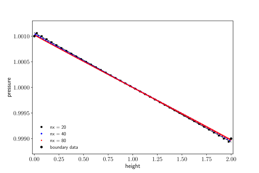
Figure 18: Mixed bounce back and anti bounce back boundary condition for linear Poiseuille flow. Pressure field for three meshes: the results are numerically convergent.

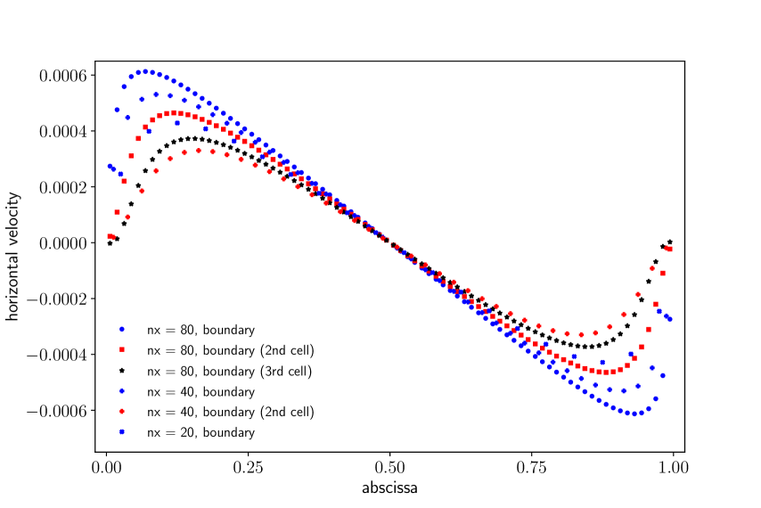
Figure 19: Mixed bounce back and anti bounce back boundary condition for linear Poiseuille flow. Horizontal velocity field for three meshes. The maximum error is reduced by one order of magnitude compared to the anti bounce back boundary scheme.

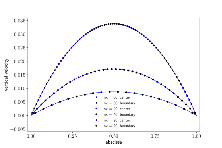
Figure 20: Mixed bounce back and anti bounce back boundary condition for linear Poiseuille flow. Vertical velocity field for three meshes. The parabolic profile is recovered in the first cell.

mesh $20\times 40$ $40\times 80$ $80\times 160$ center $4.56\,10^{-3}$ $2.40\,10^{-3}$ $1.33\,10^{-3}$ bottom $0.0165$ $0.0608$ $0.108$

Table 5: Anti bounce back boundary condition for linear Poiseuille flow. Numerical position of the boundary measured in cell units. The errors are reduced in a significative manner compared with the one obtained with the pure anti bounce boundary condition (see Table 3).

9)  Conclusion

In this contribution, we have presented the derivation of anti bounce back boundary condition in the fundamental case of linear heat conduction and linear acoustics. We have recalled that using this type of boundary condition is now classical, even in the extended version that allows taking into account curved boundaries. The asymptotic analysis confirms the high quality of the anti bounce back boundary condition for implementing a Dirichlet condition for the heat equation. For the linear fluid system, the anti bounce back boundary condition is designed for taking into account a pressure boundary condition. The asymptotic analysis puts in evidence a differential hidden condition on the boundary. For a Poiseuille flow this hidden condition induces serious discrepancies in the vicinity of the input and output. A variant mixing bounce back and anti bounce back has been proposed in order to set in a mathematical rigorous way fluid conditions composed by the datum of pressure and tangential velocity. A test case for Poiseuille flow is very encouraging.

In future works, the analysis of the pure anti bounce back for thermal problem will be extended up to order two. The novel mixing boundary condition will be investigated more precisely theoretically and numerically, in particular for unsteady acoustic problems. Moreover, the Taylor expansion method near the boundary needs to be generalized for oblique and curved boundaries. Finally a more general boundary condition has to be conceived to reduce the defects at first order and eliminate as far as possible the hidden boundary conditions.

Acknowledgments

The authors thank the referees for precise comments on the first drafts of this contribution.

References

References

[1]
[2]
S. Ansumali, I.V. Karlin,
“Kinetic Boundary Conditions in the Lattice Boltzmann Method”,
Physical Review E, vol. 66, p. 026311, 2002.
[3]
C. Bègue, C. Conca, F. Murat, O. Pironneau.
“Les équations de Stokes et de Navier-Stokes avec des conditions aux limites sur la pression”,
Nonlinear partial differential equations and their applications,
Collège de France Seminar (Paris, 1985-1986), volume IX,H. Brézis and J.L. Lions Eds,
Pitman research notes in mathematics series, vol. 181, Longman Scientific & Technical, Harlow,
p. 179-264, 1988.
[4]
M. Bouzidi, M. Firdaouss, P. Lallemand.
“Momentum transfer of a Boltzmann-lattice fluid with boundaries”,
Physics of Fluids, vol. 13, p. 3452-3459, 2001
[5]
A. P. Calderón.
“Uniqueness in the Cauchy problem for partial differential equations”,
American Journal of Mathematics, vol. 80, p. 16-36, 1958.
[6]
B. Chun, A.J.C. Ladd.
“Interpolated boundary condition for lattice Boltzmann simulations of flows in narrow gaps”,
Physical Review E, vol. 75, 066705, 2007.
[7]
D. d’Humières, , Y. Pomeau, P. Lallemand.
“Simulation d’allées de Von Karman bidimensionnelles à l’aide d’un gaz sur réseaux”, Comptes Rendus de l’Académie des Sciences de Paris, vol. 301, série II, 1985, p. 1391-1394, 1985.
[8]
D. d’Humières, I. Ginzburg,
“Multi-reflection boundary conditions for lattice Boltzmann models”,
Physical Review E, vol. 68, issue 6, p. 066614 (30 pages), 2003.
[9]
A. Douglis.
“Uniqueness in Cauchy problems for elliptic systems of equations”,
Communications on Pure and Applied Mathematics, vol. 13, p. 593-608, 1953.
[10]
F. Dubois.
“Formulation tourbillon-vitesse-pression pour le problème de Stokes”, Comptes Rendus de l’Académie des Sciences de Paris,
série 1, vol. 314, p. 277-280, 1992.
[11]
F. Dubois.
“Vorticity-velocity-pressure formulation for the Stokes problem”,
Mathematical Methods in the Applied Sciences, vol. 25, Issue 13, p. 1091-1119, 2002.
[12]
F. Dubois.
“Equivalent partial differential equations of a Boltzmann scheme”,
Computers and mathematics with applications, vol. 55,
p. 1441-1449, 2008.
[13]
F. Dubois, P. Lallemand.
“Towards higher order lattice Boltzmann schemes ”,
Journal of Statistical Mechanics: Theory and Experiment, P06006, 2009.
[14]
F. Dubois, P. Lallemand.
“Quartic Parameters for Acoustic Applications of Lattice Boltzmann Scheme”,
Computers and Mathematics with Applications, vol. 61, p. 3404-3416, 2011.
[15]
F. Dubois, P. Lallemand.
“Comparison of Simulations of Convective Flows”,
Communications in Computational Physics, vol. 17, p. 1169-1184, 2015.
[16]
F. Dubois, P. Lallemand, M. M. Tekitek,
“On a superconvergent lattice Boltzmann boundary scheme”,
Computers and Mathematics with Appls.,
vol. 59, p. 2141-2149, 2010.
[17]
F. Dubois, P. Lallemand, M.M. Tekitek.
“Taylor expansion method for analyzing bounce-back boundary conditions for lattice Boltzmann method”
ESAIM: Proceedings and Surveys, vol. 52, p. 25-46, 2015.
[18]
F. Dubois, P. Lallemand, M.M. Tekitek.
“Generalized bounce back boundary condition for the nine velocities two-dimensional
lattice Boltzmann scheme”,
“Taylor expansion method for analyzing bounce-back boundary conditions for lattice Boltzmann method”
Computers & Fluids, online 3 July 2017.
[19]
L.C. Evans.
Partial Differential Equations, American Mathematical Society, Providence, ISBN 0-8218-0772-2, 1998.
[20]
S.-D. Feng, R.-C. Ren, Z.-Z. Ji.
“Heat Flux Boundary Conditions for a Lattice Boltzmann Equation Model”,
Chinese Physics Letters, vol. 19, p. 79-82, 2002.
[21]
V. Girault, P.-A. Raviart. Finite Element Methods for Navier-Stokes Equations; Theory and Algorithms,
Springer Series in Computational Mathematics, vol. 5, 1986.
[22]
M. Hénon. “Viscosity of a Lattice Gas”, Complex Systems,
vol. 1, p. 763-789, 1987.
[23]
D. d’Humières. “Generalized Lattice-Boltzmann Equations”,
in Rarefied Gas Dynamics: Theory and Simulations,
vol. 159 of AIAA Progress in
Astronautics and Astronautics, p. 450-458, 1992.
[24]
I. Ginzburg, P. Adler.
“Boundary flow condition analysis for the three-dimensional lattice Boltzmann model”,
Journal of Physics II France, vol. 4, p. 191-214, 1994.
[25]
J. Lätt, B. Chopard, O. Malaspinas, M. Deville, A. Michler.
“Straight velocity boundaries in the lattice Boltzmann method”,
Physical Review E, vol. 77, 056703, 2008.
[26]
P. Lallemand, L.-S. Luo.
“Theory of the lattice Boltzmann method:
Dispersion, dissipation, isotropy, Galilean invariance, and stability”,
Physical Review E, vol. 61, p. 6546-6562, 2000.
[27]
R.B. Lehoucq, D.C. Sorensen, C. Yang.
ARPACK Users Guide: Solution of Large-Scale Eigenvalue Problems with Implicitly
Restarted Arnoldi Methods, ISBN 978-0-89871-407-4,
SIAM Software, Environments and Tools, Philadelphia, 1998.
[28]
A.J. Wagner, I. Pagonabarraga.
“Lees-Edwards Boundary Conditions for Lattice Boltzmann”,
Journal of Statistical Physics, vol. 107, p. 521-537, 2002.
[29] J. Wang, D. Wang, P. Lallemand, L.-S. Luo.
“Lattice Boltzmann simulations of thermal convective flows in two dimensions”,
Computers & Mathematics with Applications, vol. 65, p. 262-286, 2013.
[30]
Q. Zou, X. He.
“On pressure and velocity boundary conditions for the lattice Boltzmann BGK model”,
Physics of Fluids, vol. 9, p. 1591-1598, 1997.