Renormalization of the GT operator within the realistic shell model

Abstract

In nuclear structure calculations, the choice of a limited model space, due to computational needs, leads to the necessity to renormalize the Hamiltonian as well as any transition operator. Here, we present a study of the renormalization procedure and effects of the Gamow-Teller operator within the framework of the realistic shell model. Our effective shell-model operators are obtained, starting from a realistic nucleon-nucleon potential, by way of the many-body perturbation theory in order to take into account the degrees of freedom that are not explicitly included in the chosen model space. The theoretical effective shell-model Hamiltonian and transition operators are then employed in shell-model calculations, whose results are compared with data of Gamow-Teller transition strengths and double-$\beta$ half-lives for nuclei which are currently of interest for the detection of the neutrinoless double-$\beta$ decay process, in a mass interval ranging from $A=48$ up to $A=136$. We show that effective operators are able to reproduce quantitatively the spectroscopic and decay properties without resorting to an empirical quenching neither of the axial coupling constant $g_{A}$, nor of the spin and orbital gyromagnetic factors. This should assess the reliability of applying present theoretical tools to this problematic.

I Introduction

A long-standing issue of nuclear structure calculations is the need to reduce the number of the configurations available to the interacting nucleons, which constitute the nuclear system under investigation. Such approximations, that are necessary to overcome the computational complexity of the nuclear many-body problem, drive the nuclear structure practitioners to resort to effective Hamiltonians and operators, that depend on a certain set of parameters, built up to account for the degrees of freedom which do not appear explicitly in the calculated wavefunctions. The development of effective operators suitable to describe observables is a problematic that has to be tackled in most nuclear structure models that relies on the truncation of the number of interacting nucleons and/or the dimension of the configuration space. This issue does not affect ab initio approaches when their results are convergent with respect to the truncation of the nuclear correlations that is needed to solve the many-body Schrödinger equation (see for example Ref. Hjorth-Jensen et al. (2017)).

In the nuclear shell model (SM), the physics of a certain nuclear system is described in terms only of a limited number of valence nucleons, that interact in a model space consisting of a major shell, placed outside a closed core made up by the remaining constituent nucleons, the latter being frozen inside a number of filled shells.

The status of the theoretical derivation of an effective shell-model Hamiltonian ($H_{\rm eff}$), starting from a realistic nuclear potential, has reached nowadays a notable progress, especially within the framework of the many-body perturbation theory Hjorth-Jensen et al. (1995); Coraggio et al. (2012). At present, realistic shell-model Hamiltonians are largely employed in shell-model calculations, exhibiting a substantial reliability (see, for example Ref. Coraggio et al. (2009) and references therein).

As regards the theoretical efforts to derive effective shell-model transition operators starting from realistic potentials, the literature is far less extended, but it is worth mentioning an early review about this topic, which can be found in Ref. Ellis and Osnes (1977). More recently, Suzuki and Okamoto have developed a formalism to derive effective shell-model operators Suzuki and Okamoto (1995), that provides an approach that is consistent with the construction of the corresponding $H_{\rm eff}$.

In the present work we focus on the derivation of effective shell-model Gamow-Teller (GT) operators to calculate observables related to the $\beta$-decay transition for nuclei in different mass regions, aiming to trace back to the roots of the quenching of the free value of the axial coupling constant $g_{A}$ in nuclear structure calculations.

It should be mentioned that similar studies have been reported in Refs. Siiskonen et al. (2001); Holt and Engel (2013). In Ref. Siiskonen et al. (2001), the renormalization of the GT operator, in the form of a one-body operator, has been carried out to study the role of the weak hadronic current in the nuclear medium. The authors of Ref. Holt and Engel (2013) have instead calculated nuclear matrix elements of the two-neutrino double-$\beta$ decay ($2\nu\beta\beta$) building an effective two-body operator within the so-called closure approximation.

As a matter of fact, effective GT operators are in general obtained resorting to effective values of $g_{A}$, via a quenching factor $q$, to reproduce experimental GT transitions. The choice of $q$ depends obviously on the nuclear structure model employed to derive the nuclear wave functions, the dimensions of the considered Hilbert space, and the mass of the nucleus under investigation.

This problem, which affects the calculations of the Gamow-Teller transition strengths and double-$\beta$ half-lives, has been investigated within different nuclear-structure models, such as the Interacting Boson Model Barea and Iachello (2009); Barea et al. (2012, 2013), the Quasiparticle Random-Phase Approximation Šimkovic et al. (2008, 2009); Fang et al. (2011); Faessler et al. (2012); Šimkovic et al. (2018), and the Shell Model Caurier et al. (2008); Menéndez et al. (2009a, b); Caurier et al. (2012); Horoi et al. (2007); Horoi (2013a); Horoi and Brown (2013); Neacsu and Horoi (2015); Brown et al. (2015); Iwata et al. (2016). In this regard, it is worth mentioning the recent review paper by Suhonen Suhonen (2017a), where the quenching is discussed from the points of view of the different methods.

For the sake of clarity, we point out that the quenching of $g_{A}$ is entangled with both the renormalization of many-body correlations - due to the truncation of the basis used to construct the wave functions - and the corrections due to the subnucleonic structure of the nucleons Park et al. (1993); Pastore et al. (2009); Piarulli et al. (2013); Baroni et al. (2016a), since the free value $g_{A}^{free}=1.2723$ Tanabashi et al. (2018) is obtained from the data of the neutron decay under the assumption that the nucleons are point-like particles.

We will show in the following that the perturbative approach to the derivation of effective spin-dependent operators allows to reproduce quantitatively spectroscopic and decay properties without resorting to an empirical quenching neither of the axial coupling constant $g_{A}$, nor of the spin and orbital $g$-factors.

In this connection, it is worth noting that an important contribution to understand the quenching of $g_{A}$ within a microscopic framework has been given by the studies of I. S. Towner and co-workers (see the review paper Towner (1987) and references therein), who have extensively investigated the role played by both the many-body correlations induced by the truncation of the Hilbert space and the two-body meson-exchange currents in the renormalization of spin-dependent electromagnetic ($M1$) and weak (GT) operators Towner and Khanna (1983).

Nowadays, there is a renewed interest in the problematics of the renormalization of the GT operator, because of its connection with the calculation of the nuclear matrix elements (NME) of the $0\nu\beta\beta$ decay (see for example Ref. Suhonen (2017b)). In fact, the half life of such a process is expressed by:

$$\left[T^{0\nu}_{1/2}\right]^{-1}=G^{0\nu}\left|M^{0\nu}\right|^{2}\langle m_{\nu}\rangle^{2}~{}~{},$$ (1)

where $G^{0\nu}$ is the so-called phase-space factor, $\langle m_{\nu}\rangle$ is the effective neutrino mass, and $M^{0\nu}$ is the nuclear matrix element, that relates the wave functions of the parent and grand-daughter nuclei. As a matter of fact, $M^{0\nu}$ can be expressed as the sum of the GT, Fermi (F), and tensor (T) matrix elements, and depends on the axial and vector coupling constants $g_{A},g_{V}$ :

$$M^{0\nu}=M^{0\nu}_{GT}-\left(\frac{g_{V}}{g_{A}}\right)^{2}M^{0\nu}_{F}-M^{0\nu}_{T}~{}~{}.$$ (2)

On these grounds, we focus attention on the renormalization of the GT operator that takes into account the reduced SM model space, without considering the corrections arising from meson-exchange currents Towner and Khanna (1983); Baroni et al. (2016b). Our theoretical framework is the many-body perturbation theory Kuo et al. (1981); Suzuki and Okamoto (1995); Coraggio et al. (2012, 2017), and, starting from a realistic nuclear potential, we derive effective shell-model GT operators and Hamiltonians for nuclei with mass ranging from $A=48$ to $A=136$. We also consider in the derivation of the one-body effective operators the so-called “blocking effect”, to take into account the Pauli exclusion principle in systems with more than one valence nucleon Ellis and Osnes (1977).

In Section II we will sketch out a few details about the derivation of the effective SM Hamiltonians and operators from a realistic nucleon-nucleon ($NN$) interaction. The results of the shell-model calculations are then reported in Section III. More precisely, we compare calculated and experimental $2\nu\beta\beta$-decay matrix elements, GT transition-strength distributions for nuclei that are candidates for the detection of the $0\nu\beta\beta$-decay. We extend this analysis to magnetic dipole moments and reduced transition probabilities ($B(M1)$), and, for the sake of completeness, the energy spectra and $B(E2)$ values of the parent and grand-daughter nuclei are also shown. The conclusions of this study are drawn in Section IV, together with the outlook of our current project. In Appendix, tables containing the calculated SP energies of the effective Hamiltonians and the matrix elements of the effective $M1$ and GT operators are reported.

II Outline of calculations

The cornerstone of a realistic shell-model calculation is the choice of a realistic nuclear potential to start with. We consider for our calculations the high-precision CD-Bonn $NN$ potential Machleidt (2001), whose non-perturbative behavior requires to integrate out its repulsive high-momentum components by way of the so-called $V_{\rm low-k}$ approach Bogner et al. (2001, 2002). This is based on a unitary transformation that provides a softer nuclear potential defined up to a cutoff $\Lambda$, and preserves the physics of the original CD-Bonn interaction.

As in our recent works Coraggio et al. (2015a, b); Coraggio et al. (2016, 2017), the value of the cutoff $\Lambda$ is chosen equal to 2.6 fm^-1, since we have found that the role of missing three-nucleon force (3NF) decreases by enlarging the $V_{\rm low-k}$ cutoff Coraggio et al. (2015b). In our experience, $\Lambda=2.6$ fm^-1 is an upper limit, since with a larger cutoff the order-by-order behavior of the perturbative expansion may be not satisfactory.

This $V_{\rm low-k}$ is then employed as the two-body interaction term of the Hamiltonian for the system of $A$ nucleons under investigation:

$$H=\sum_{i=1}^{A}\frac{p_{i}^{2}}{2m}+\sum_{i<j=1}^{A}V_{\rm low-k}^{ij}=T+V_{\rm low-k}~{}~{}.$$ (3)

This Hamiltonian should be then diagonalized in an infinite Hilbert space to describe the physical observables. Obviously, this task is unfeasible, and in the shell model the infinite number of degrees of freedom is reduced only to those characterizing the physics of a limited number of interacting nucleons, that are constrained in a finite Hilbert space spanned by a few accessible orbitals. To this end, the Hamiltonian $H$ of Eq. 3 is broken up, by way of an auxiliary one-body potential $U$, into the sum of a one-body term $H_{0}$, whose eigenvectors set up the shell-model basis, and a residual interaction $H_{1}$:

$$H = T+V_{\rm low-k}=(T+U)+(V_{\rm low-k}-U)=$$

$$= H_{0}+H_{1}~{}~{}.$$ (4)

The following step is to derive an effective shell-model Hamiltonian $H_{\rm eff}$, that takes into account the degrees of freedom that are not explicitly included in the shell-model framework, as the core polarization due to the interaction, within the full Hilbert space, between the valence nucleons and those belonging to the closed core.

We derive $H_{\rm eff}$ by resorting to the many-body perturbation theory, an approach that has been developed by Kuo and coworkers through the 1970s Kuo and Osnes (1990); Kuo et al. (1995). More precisely, we use the well-known $\hat{Q}$ box-plus-folded-diagram method Kuo et al. (1971), where the $\hat{Q}$ box is defined as a function of the unperturbed energy $\epsilon$ of the valence particles:

$$\hat{Q}(\epsilon)=PH_{1}P+PH_{1}Q\frac{1}{\epsilon-QHQ}QH_{1}P~{}~{},$$ (5)

where the operator $P$ projects onto the model space and $Q=\mathbf{1}-P$. In the present calculations the $\hat{Q}$ box is expanded as a collection of one- and two-body irreducible valence-linked Goldstone diagrams up to third order in the perturbative expansionCoraggio et al. (2010, 2012).

Within this framework the effective Hamiltonian $H_{\rm eff}$ can be written in an operator form as

$$H_{\rm eff}=\hat{Q}-\hat{Q^{\prime}}\int\hat{Q}+\hat{Q^{\prime}}\int\hat{Q}\int\hat{Q}-\hat{Q^{\prime}}\int\hat{Q}\int\hat{Q}\int\hat{Q}+~{}...~{}~{},$$ (6)

where the integral sign represents a generalized folding operation Brandow (1967), and $\hat{Q^{\prime}}$ is obtained from $\hat{Q}$ by removing first-order terms Krenciglowa and Kuo (1974).

Since it has been demonstrated the following operatorial identity Krenciglowa and Kuo (1974):

$$\hat{Q}\int\hat{Q}=-\hat{Q}_{1}\hat{Q}~{}~{},$$ (7)

the solution of Eq. 6 may be obtained using the $\hat{Q}$ box derivatives

$$\hat{Q}_{m}=\frac{1}{m!}\frac{d^{m}\hat{Q}(\epsilon)}{d\epsilon^{m}}\biggl{|}_{\epsilon=\epsilon_{0}}~{}~{},$$ (8)

$\epsilon_{0}$ being the model-space eigenvalue of the unperturbed Hamiltonian $H_{0}$, that we have chosen to be harmonic-oscillator (HO) one.

Consequently, the expression in Eq. 6 may be rewritten as

$$H_{\rm eff}=\sum_{i=0}^{\infty}F_{i}~{}~{},$$ (9)

where

$$F_{0} = \hat{Q}(\epsilon_{0})$$

$$F_{1} = \hat{Q}_{1}(\epsilon_{0})\hat{Q}(\epsilon_{0})$$

$$F_{2} = \left[\hat{Q}_{2}(\epsilon_{0})\hat{Q}(\epsilon_{0})+\hat{Q}_{1}(\epsilon_{0})\hat{Q}_{1}(\epsilon_{0})\right]\hat{Q}(\epsilon_{0})$$

$$...$$ (10)

From $H_{\rm eff}$ for one-valence-nucleon systems we obtain the single-particle (SP) energies for our SM calculations, while the two-body matrix elements (TBMEs) are obtained from $H_{\rm eff}$ derived for the nuclei with two valence nucleons, by subtracting the theoretical SP energies. The calculated SP energies for ⁴⁰Ca, ⁵⁶Ni, and ¹⁰⁰Sn cores are reported in the Appendix, while the corresponding TBMEs can be found in the Supplemental Material sup .

A detailed description of the perturbative properties of our $H_{\rm eff}$, derived from the same $V_{\rm low-k}$ of present work, can be found in Coraggio et al. (2018), where it has been reported the behavior of SP energies and TBME as a function of both the perturbative order and the number of the intermediate states.

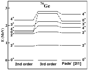
Figure 1: Calculated spectra of ⁷⁶Ge obtained from the perturbative expansion of $H_{\rm eff}$ using $\hat{Q}$-box diagrams up to second-, third-order, and Padé approximant $[2|1]$ (see text for details).

In order to exemplify pictorially the impact of the perturbation expansion on the energy spectra, we report in Fig. 1 the low-energy spectra of ⁷⁶Ge obtained with $H_{\rm eff}$s derived from $\hat{Q}$-boxes at second-, third-order in perturbation theory, and their Padé approximant $[2|1]$ Baker and Gammel (1970). We employ the Padé approximant in order to obtain a better estimate of the convergence value of the perturbation series Coraggio et al. (2012), as suggested in Hoffmann et al. (1976). As can be seen, a rather good convergence is obtained, apart from the second-excited $J^{\pi}=0^{+}$ state, the largest discrepancy occurring for the yrare $J^{\pi}=4^{+}$ that is about $20\%$ from second to third order and $6\%$ from third order to Padé approximant $[2|1]$.

As mentioned before, we derive the effective transition operators, namely the matrix elements of the effective spin-dependent $M1$, GT operators and the effective charges of the electric quadrupole operator, using the formalism presented by Suzuki and Okamoto in Ref. Suzuki and Okamoto (1995).

As a matter of fact, a non-Hermitian effective operator $\Theta_{\rm eff}$ can be expressed in terms of the $\hat{Q}$ box, its derivatives, and an infinite sum of operators $\chi_{n}$, the latter being defined as:

$$\chi_{0} = (\hat{\Theta}_{0}+h.c.)+\hat{\Theta}_{00}~{}~{},$$ (11)

$$\chi_{1} = (\hat{\Theta}_{1}\hat{Q}+h.c.)+(\hat{\Theta}_{01}\hat{Q}+h.c.)~{}~{},$$ (12)

$$\chi_{2} = (\hat{\Theta}_{1}\hat{Q}_{1}\hat{Q}+h.c.)+(\hat{\Theta}_{2}\hat{Q}\hat{Q}+h.c.)+$$

$$(\hat{\Theta}_{02}\hat{Q}\hat{Q}+h.c.)+\hat{Q}\hat{\Theta}_{11}\hat{Q}~{}~{},$$

$$\cdots$$

where $\hat{\Theta}_{m}$, $\hat{\Theta}_{mn}$ have the following expressions:

$$\hat{\Theta}_{m} = \frac{1}{m!}\frac{d^{m}\hat{\Theta}(\epsilon)}{d\epsilon^{m}}\biggl{|}_{\epsilon=\epsilon_{0}}~{}~{}~{},$$ (14)

$$\hat{\Theta}_{mn} = \frac{1}{m!n!}\frac{d^{m}}{d\epsilon_{1}^{m}}\frac{d^{n}}{d\epsilon_{2}^{n}}\hat{\Theta}(\epsilon_{1};\epsilon_{2})\biggl{|}_{\epsilon_{1}=\epsilon_{0},\epsilon_{2}=\epsilon_{0}}~{},$$ (15)

with

$$\hat{\Theta}(\epsilon)= P\Theta P+P\Theta Q\frac{1}{\epsilon-QHQ}QH_{1}P~{},~{}~{}~{}~{}~{}~{}~{}~{}~{}~{}~{}~{}~{}~{}~{}~{}~{}~{}~{}$$ (16)

$$\hat{\Theta}(\epsilon_{1};\epsilon_{2})= PH_{1}Q\frac{1}{\epsilon_{1}-QHQ}Q\Theta Q\frac{1}{\epsilon_{2}-QHQ}QH_{1}P~{},~{}~{}~{}~{}~{}$$ (17)

$\Theta$ being the bare transition operator.

The effective transition operators can be written, in terms of the above quantities, as follows

$$\Theta_{\rm eff} = (P+\hat{Q}_{1}+\hat{Q}_{1}\hat{Q}_{1}+\hat{Q}_{2}\hat{Q}+\hat{Q}\hat{Q}_{2}+\cdots)$$

$$\times(\chi_{0}+\chi_{1}+\chi_{2}+\cdots)~{}~{}.$$ (18)

Now, inserting the identity $\hat{Q}\hat{Q}^{-1}=\mathbf{1}$ and taking into account Eqs. 9, 10, Eq. 18 may be then recast in the following form

$$\Theta_{\rm eff} = (P+\hat{Q}_{1}+\hat{Q}_{1}\hat{Q}_{1}+\hat{Q}_{2}\hat{Q}+\hat{Q}\hat{Q}_{2}+\cdots)\hat{Q}\hat{Q}^{-1}$$

$$\times(\chi_{0}+\chi_{1}+\chi_{2}+\cdots)=$$

$$= H_{\rm eff}\hat{Q}^{-1}(\chi_{0}+\chi_{1}+\chi_{2}+\cdots)~{}~{},$$ (19)

The above form provides a strong link between the derivation of the effective Hamiltonian and all effective operators.

In our calculations for the aforementioned one-body transition operators, we arrest the $\chi_{n}$ series to the $\chi_{2}$ term. It is worth reminding that in Refs. Coraggio et al. (2017, 2018) we have included only the leading term $\chi_{0}$. The calculation is performed starting from a perturbative expansion of $\hat{\Theta}_{0}$ and $\hat{\Theta}_{00}$, including diagrams up to the third order in the perturbation theory, consistently with the perturbative expansion of the $\hat{Q}$ box. We have found that $\chi_{2}$ contribution is at most $1\%$ of the final results. Since $\chi_{3}$ depends on the first, second, and third derivatives of $\hat{\Theta}_{0}$ and $\hat{\Theta}_{00}$, and on the first and second derivatives of the $\hat{Q}$ box (see Eq. II), our estimation of these quantities leads to evaluate $\chi_{3}$ being at least one order of magnitude smaller than $\chi_{2}$.

For the sake of clarity, in Fig. 2 we report all the one-body $\Theta_{0}$ diagrams up to the second order, the bare operator $\Theta$ being represented with an asterisk. The first-order $(V_{\rm low-k}-U)$-insertion, represented by a circle with a cross inside, arises because of the presence of the $−U$ term in the interaction Hamiltonian $H_{1}$ (see for example Ref. Coraggio et al. (2012) for details).

In Ref. Coraggio et al. (2018) we have carried out a study of the perturbative properties of the GT operator for the calculation of the NME ($M_{\rm GT}^{2\nu}$) of the ¹³⁰Te, ¹³⁶Xe $2\nu\beta\beta$ decay. We have found that the results for the ¹³⁰Te decay vary by about $10\%$ from second to third order in perturbation theory, and that for ¹³⁶Xe by about $5\%$.

As regards the magnetic-dipole operator, we find a similar perturbative behavior. As a matter of fact, the calculated magnetic dipole moments of the yrast $J^{\pi}=2^{+}$ states in ¹³⁰Te and ¹³⁶Xe, obtained with an effective operator derived at second order in perturbation theory, are 0.65 and 1.19 $\mu_{N}$, respectively, to be compared with 0.71 and 1.15 $\mu_{N}$ at third-order (see also Tables 7,9.) The variation from second to third order is about $8\%$ for ¹³⁰Te, and $3\%$ for ¹³⁶Xe.

Figure 2: One-body second-order diagrams included in the perturbative expansion of $\hat{\Theta}$. The asterisk indicates the bare operator $\Theta$, the wavy lines the two-body potential $V_{\rm low-k}$.

The authors of Ref. Siiskonen et al. (2001) have carried out a perturbative expansion of the $\hat{\Theta}$ operator for GT transitions in terms of similar diagrams, calculated up to third-order in perturbation theory and employing $G$-matrix energy-dependent interaction vertices. They have added to them the corresponding folded diagrams according to the prescription of Ref. Towner (1987), but have neglected all diagrams with $(G-U)$-insertion vertices, which - it is worth to point out - at second order only are equal to zero for spin-dependent operators.

They have reported a selection of the matrix elements of their effective GT⁺ operator, that we compare with our results in Tables A.VII,A.VIII, and A.IX. As can be observed, both calculations provide consistent results, even if some matrix elements differ up to $25\%$.

The topology of the diagrams reported in Fig. 2 deals, obviously, with single-valence nucleon systems, and many-body diagrams should be included starting from nuclei with two valence nucleons on; in Fig. 3 we report all two-valence-nucleon diagrams for one-body operators, up to second order of the $\hat{\Theta}$ perturbative expansion. For the sake of simplicity, for each topology we draw only one of the diagrams which correspond to the exchange of the external pairs of lines.

Diagrams (a)-(d) are the same as in Fig. 2 but with a spectator line $a$, while connected diagrams ($\mathrm{d}_{1}$) and ($\mathrm{d}_{2}$) correct Pauli-principle violation introduced by diagram (d) when the particles $c$ and $p$ own the same quantum numbers.

Figure 3: Two-body second-order diagrams that should appear in the perturbative expansion of $\chi_{0}$. As in Fig. 2, the asterisk indicates the bare operator $\Theta$, the wavy lines the two-body potential $V_{\rm low-k}$.

Since it is straightforward to perform shell-model calculations using one-body transition operators, we derive a density-dependent one-body operator from the two-body ones by summing and averaging over one incoming and outcoming particles of the connected diagrams ($\mathrm{d}_{1}$) and ($\mathrm{d}_{2}$) of Fig. 3. This allows to take into account the filling of the model-space orbitals when dealing with more than one valence nucleon.

Figure 4: Density-dependent one-body second-order diagram $(I)$ that is obtained from diagram $(\mathrm{d}_{1})$ of Fig. 2 by summing over one incoming and outcoming particles of the two-body diagram (see text for details).

For example, we report in Fig. 4 the second-order density-dependent one-body diagram ($I$), obtained from the contribution ($\mathrm{d}_{1}$) of Fig. 3, and whose explicit expression is

$$(I)=\sum_{\alpha}\sum_{pJ}\frac{(2J+1)}{(2j_{b}+1)}\frac{\langle a||\Theta||p\rangle\langle p\alpha,J|V_{\rm low-k}|b\alpha,J\rangle}{(\epsilon_{b}-\epsilon_{p})}\rho(\alpha)~{}~{},$$ (20)

where $\alpha$ and $p$ indices run over the orbitals in, and above the model space, respectively, the matrix elements of the $V_{\mathrm{l}ow-k}$ are coupled to the total angular momentum $J$, $\epsilon_{i}$ stands for the unperturbed energy of the orbital $i$, and $\rho(\alpha)$ is the occupation probability of the orbital $\alpha$.

In this work all the results of the shell-model calculations, that are shown in Sec. III, have been obtained employing SP energies, TBMEs, and effective one-body operators derived by way of the above mentioned theoretical approach, including consistently all contributions up to third-order in the perturbative expansion, without resorting to any empirically fitted parameter.

In Sec. III, the calculated running sums of the GT strengths ($\Sigma B(p,n)$), obtained with both bare and effective GT operators, are reported as a function of the excitation energy, and compared with the available data extracted from experiment. The GT strength is defined as follows:

$$B(p,n)=\frac{\left|\langle\Phi_{f}||\sum_{j}\vec{\sigma}_{j}\tau^{-}_{j}||\Phi_{i}\rangle\right|^{2}}{2J_{i}+1}~{}~{},$$ (21)

where indices $i,f$ refer to the parent and grand-daughter nuclei, respectively, and the sum is over all interacting nucleons.

The single-$\beta$ decay GT strengths, defined by Eq. (21), can be accessed experimentally through intermediate energy charge-exchange reactions, since the $\beta$-decay process is forbidden for the nuclei under our investigation. The GT strength can be extracted from the GT component of the cross section at zero degree, following the standard approach in the distorted-wave Born approximation (DWBA) Goodman et al. (1980); Taddeucci et al. (1987):

$$\frac{d\sigma^{GT}(0^{\circ})}{d\Omega}=\left(\frac{\mu}{\pi\hbar^{2}}\right)^{2}\frac{k_{f}}{k_{i}}N^{\sigma\tau}_{D}|J_{\sigma\tau}|^{2}B(p,n)~{}~{},$$ (22)

where $N^{\sigma\tau}_{D}$ is the distortion factor, $|J_{\sigma\tau}|$ is the volume integral of the effective $NN$ interaction, $k_{i}$ and $k_{f}$ are the initial and final momenta, respectively, and $\mu$ is the reduced mass.

As regards the calculation of the NME of the $2\nu\beta\beta$ decay, it can be obtained via the following expression:

$$M_{\rm GT}^{2\nu}=\sum_{n}\frac{\langle 0^{+}_{f}||\vec{\sigma}\tau^{-}||1^{+}_{n}\rangle\langle 1^{+}_{n}||\vec{\sigma}\tau^{-}||0^{+}_{i}\rangle}{E_{n}+E_{0}}~{}~{},$$ (23)

where $E_{n}$ is the excitation energy of the $J^{\pi}=1^{+}_{n}$ intermediate state, $E_{0}=\frac{1}{2}Q_{\beta\beta}(0^{+})+\Delta M$, $Q_{\beta\beta}(0^{+})$ and $\Delta M$ being the $Q$ value of the $\beta\beta$ decay and the mass difference between the daughter and parent nuclei, respectively. In the above equation the index $n$ runs over all possible intermediate states of the daughter nucleus. The NMEs have been calculated using the ANTOINE shell-model code, using the Lanczos strength-function method as in Ref. Caurier et al. (2005), and including as many as intermediate states to obtain at least a four-digit accuracy (see also Figs. 5,11 in Ref. Coraggio et al. (2017)). The theoretical values are then compared with the experimental counterparts, that are extracted from the observed half life $T^{2\nu}_{1/2}$

$$\left[T^{2\nu}_{1/2}\right]^{-1}=G^{2\nu}\left|M_{\rm GT}^{2\nu}\right|^{2}~{}~{}.$$ (24)

The calculation of $M_{\rm GT}^{2\nu}$ may be also performed without calculating explicitly the intermediate $J^{\pi}=1^{+}_{n}$ states of the daughter nucleus, namely resorting to the so-called closure approximation Haxton and Stephenson Jr. (1984). The price to be payed is that the transition operator is no longer a one-body operator but a two-body one. It is worth pointing out that this approximation is largely employed to calculate the $0\nu\beta\beta$ NME ($M^{0\nu}$), since the high momentum of the neutrino - which appears explicitly in the definition of $M^{0\nu}$ - is about 100 MeV that is one order of magnitude greater than the average $J^{\pi}=1^{+}_{n}$ excitation energy. As a matter of fact, it has been estimated that this approximation is valid within $10\%$ of the exact result Sen’kov and Horoi (2013). Actually, the same approximation has turned out to be very unsatisfactory for the calculation of $M_{\rm GT}^{2\nu}$, because the energies of the neutrinos which are emitted in the $2\nu\beta\beta$ process are much smaller. For instance, in Ref. Holt and Engel (2013) the authors obtain a result for ⁷⁶Ge $M_{\rm GT}^{2\nu}$ that is about two times larger than the one calculated with the Lanczos strength-function method by employing the same SM wave functions Horoi (2013b); Brown et al. (2015), and about 5 times larger than the experimental value Barabash (2015).

III Results

In this section we present the results of our SM calculations.

We compare the calculated low-energy spectra of ⁴⁸Ca, ⁴⁸Ti, ⁷⁶Ge, ⁷⁶Se, ⁸²Se, ⁸²Kr, ¹³⁰Te, ¹³⁰Xe, ¹³⁶Xe, and ¹³⁶Ba, and their electromagnetic properties with the available experimental counterparts. As mentioned in the Introduction, special attention will be focussed on the magnetic dipole properties, since both $M1$ and GT operators are spin dependent.

We show also the results of the GT^- strength distributions and the calculated NMEs of the $2\nu\beta\beta$ decays for ⁴⁸Ca, ⁷⁶Ge, ⁸²Se, ¹³⁰Te, and ¹³⁶Xe, and compare them with the available data. All the calculations have been performed employing theoretical SP energies, TBMEs, and effective transition operators. In particular, for the $M1$ and GT properties we report the calculated values obtained by using the bare (I) and effective (II) operators, as well as those including the blocking effect - and labelled as (III) - by way of a density-dependent effective operator as mentioned in Sec. II. The latter give us the opportunity to investigate the role of many-body correlations on the spin- and spin-isospin-dependent one-body operators in nuclei with more than one valence nucleon.

III.1 ⁴⁸Ca

The shell-model calculation for ⁴⁸Ca and ⁴⁸Ti are performed within the full $fp$ shell, namely the proton and neutron $0f_{7/2}$, $0f_{5/2}$, $1p_{3/2}$, and $1p_{1/2}$ orbitals. In Fig. 5, we show the experimental ens ; xun and calculated low-energy spectra of ⁴⁸Ca and ⁴⁸Ti. Next to the arrows, that are proportional to the $B(E2)$ strengths, we report the explicit experimental ens ; xun and calculated $B(E2)$s in $e^{2}{\rm fm}^{4}$.

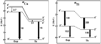
Figure 5: Experimental and calculated spectra of ⁴⁸Ca and ⁴⁸Ti. $B(E2)$ strengths (in $e^{2}{\rm fm}^{4}$) are also reported (see text for details).

As can be seen, we do not reproduce the observed shell-closure of the neutron $0f_{7/2}$ orbital in ⁴⁸Ca and the agreement between the experimental and calculated spectra is only qualitative, while experimental $B(E2)$s are satisfactorily reproduced by the theory.

In Table 1 the low-energy experimental and calculated observable related to the $M1$ operator are reported. The calculated values reported in columns I, II, III are obtained with the bare magnetic-dipole operator, the effective one without blocking effect, and the one including the blocking effect, respectively.

Table 1: Experimental and calculated $B(M1)$ strengths (in $\mu_{N}^{2}$) and magnetic dipole moments (in $\mu_{N}$) of ⁴⁸Ca and ⁴⁸Ti. We report those for the observed states in Fig. 5 (see text for details).

Nucleus	$J_{i}\rightarrow J_{f}$	$B(M1)_{\rm Expt}$	I	II	III
48Ca
	$3^{+}_{1}\rightarrow 2^{+}_{1}$	$0.023\pm 0.004$ Vanhoy et al. (1992)	0.051	0.046	0.046
Nucleus	$J$	$\mu_{\rm Expt}$	I	II	III
48Ti
	$2^{+}_{1}$	$+0.78\pm 0.04$ ens	+0.37	+0.54	+0.54
		$+0.9\pm 0.4$ ens
	$4^{+}_{1}$	$+2.2\pm 0.5$ ens	+1.2	+1.5	+1.5

From inspection of Table 1, it can be seen that the calculated magnetic-dipole transition rates $B(M1)$s compare well with the observed value for ⁴⁸Ca. In particular, from Table A.IV, the values obtained employing the effective shell-model operators (II-III) are quenched with respect to that calculated with the bare operator (I), and in a better agreement with experiment. The blocking effect is very tiny because the number of valence nucleons is rather small compared with the full capacity of the $fp$ shell.

As regards the magnetic moments, data are available for ⁴⁸Ti, and they are underestimated by the theory. However, the contribution due to the effective operators points in the right direction, leading to a better agreement with experiment.

Table 2: Experimental Barabash (2015) and calculated NME of the $2\nu\beta\beta$ decay (in MeV^-1) for ⁴⁸Ca. The same notation of Table 1 is used (see text for details).

Decay	NMEExpt	I	II	III
48Ca $\rightarrow$ 48Ti	$0.038\pm 0.003$	0.030	0.026	0.026

In Table 2 we report the observed and calculated values of the NMEs for the $2\nu\beta\beta$ decay of ⁴⁸Ca into ⁴⁸Ti. The NME obtained with the bare operator (I) slightly underestimates the experimental one, and it is $20\%$ larger than those obtained with the effective operators (II) and (III). This corresponds to a quenching factor $q=0.9$, that is roughly the average value of the reduction factor that can be extracted from Table A.VII, comparing the single-particle elements of the bare GT operator with the effective ones. In this context, it should be mentioned that our $2\nu\beta\beta$ NME calculated with the bare operator is very different from those obtained by way of SM calculations employing phenomenological $H_{\rm eff}$ Horoi et al. (2007); Caurier et al. (2012), which reproduce correctly the observed shell-closure of $0f_{7/2}$ orbital in ⁴⁸Ca.

It is worth noting that, as for the M1 properties, the blocking effect plays a negligible role also in the calculation of the $2\nu\beta\beta$ NME.

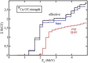
Figure 6: Running sums of the ⁴⁸Ca $B(p,n)$ strengths as a function of the excitation energy $E_{x}$ up to 5 MeV (see text for details).

In Fig. 6, the calculated $\Sigma B(p,n)$ for ⁴⁸Ca are shown as a function of the excitation energy, and compared with the data reported with a red line Yako et al. (2009). The results obtained with the bare operator (I) are drawn with a blue line, while those obtained employing the effective GT operators without and with the blocking effect are plotted using continuous and dashed black lines, respectively.

It can be seen that the distribution obtained using the bare operator (I) overestimates the observed one, and it is very close to those provided by both the effective GT operators (II-III), the blocking effect being almost negligible. Finally, we report about the theoretical total ${\rm GT}^{-}$ strengths that are 24.0, 23.1, and 23.0 with the bare operator (I), and the effective ones (II) and (III), respectively.

III.2 ⁷⁶Ge

The shell-model calculation for ⁷⁶Ge and ⁷⁶Se are performed within the model space spanned by the four proton and neutron orbitals $0f_{5/2}$, $1p_{3/2}$, $1p_{1/2}$ and $0g_{9/2}$, considering ⁵⁶Ni as closed core. The experimental ens ; xun and calculated low-energy spectra of ⁷⁶Ge and ⁷⁶Se are reported in Fig. 7, together with the experimental ens ; xun and calculated $B(E2)$ strengths (in $e^{2}{\rm fm}^{4}$), as in Fig. 5

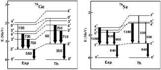
Figure 7: Same as in Fig. 5, but for ⁷⁶Ge and ⁷⁶Se (see text for details).

The agreement between the experimental and calculated spectra and $B(E2)$s is far more satisfactory than that obtained for $A=48$.

In Table 3 we report the experimental and calculated $B(M1)$ strengths as well as magnetic dipole moments of ⁷⁶Ge and ⁷⁶Se.

Table 3: Same as in Table 1, but for ⁷⁶Ge and ⁷⁶Se (see text for details).

Nucleus	$J_{i}\rightarrow J_{f}$	$B(M1)_{\rm Expt}$	I	II	III
76Ge
	$2^{+}_{2}\rightarrow 2^{+}_{1}$	$0.003^{+0.002}_{-0.003}$ Mukhopadhyay et al. (2017)	0.006	0.004	0.005
	$4^{+}_{2}\rightarrow 3^{+}_{1}$	$0.02\pm 0.01$ Mukhopadhyay et al. (2017)	0.062	0.027	0.025
		$0.002\pm 0.001$ Mukhopadhyay et al. (2017)
	$4^{+}_{2}\rightarrow 4^{+}_{1}$	$0.03^{+0.02}_{-0.03}$ Mukhopadhyay et al. (2017)	0.07	0.03	0.03
		$0.04\pm 0.02$ Mukhopadhyay et al. (2017)
Nucleus	$J$	$\mu_{\rm Expt}$	I	II	III
76Ge
	$2^{+}_{1}$	$+0.64\pm 0.02$ Gürdal et al. (2013)	+0.53	+0.83	+0.84
	$2^{+}_{2}$	$+0.78\pm 0.10$ Gürdal et al. (2013)	+0.93	+1.10	+1.09
	$4^{+}_{1}$	$+0.96\pm 0.68$ Gürdal et al. (2013)	+0.58	+1.33	+1.36
76Se
	$2^{+}_{1}$	$0.81\pm 0.05$ Speidel et al. (1998)	+0.37	+0.60	+0.58
	$2^{+}_{2}$	$0.70\pm 0.12$ Speidel et al. (1998)	+0.64	+0.82	+0.79
	$4^{+}_{1}$	$2.6\pm 0.4$ Speidel et al. (1998)	+0.3	+0.9	+0.9

It can be observed that, with respect to the calculations for ⁴⁸Ca and ⁴⁸Ti, now the contribution arising from an effective transition operator - whose matrix elements are reported in Table A.V - is more relevant, and significantly improves the comparison with data. This traces back to the fact that, as it is well known Towner (1987), spin- and spin-isospin-dependent operators need larger renormalizations when orbitals belonging to the model space lack their spin-orbit counterpart. As a matter of fact, this regards single-body matrix elements of the effective $M1$ - and GT operators - involving the $0f_{5/2}$ and $0g_{9/2}$ orbitals. We observe that also for ⁷⁶Ge and ⁷⁶Se, the blocking effect on the $M1$ operator seems rather unimportant.

As regards the comparison with experiment, both calculated $B(M1)$s and dipole moments agree with data, especially those obtained with the effective operators (II) and (III). It is worth pointing out that, using the effective operators, the quenching of the non-diagonal one-body matrix elements in Table A.V is responsible for the reduction of the calculated $B(M1)$s with respect to those obtained with the bare operator. On the other side, the enhancement of the proton diagonal matrix element $\langle 0f_{5/2}||M1||0f_{5/2}\rangle$ (see Table A.V) leads to an increase of the magnetic dipole moments of the yrast states.

As can be seen in Table A.VIII, the renormalization effect of the GT operator is even much stronger than that observed for the $M1$ operator. This is reflected in our shell-model results for the NMEs of the $2\nu\beta\beta$ decay of ⁷⁶Ge into ⁷⁶Se, that are compared with the experimental value Barabash (2015) in Table 4.

Table 4: Same as in Table 2, but for the $2\nu\beta\beta$ decay of ⁷⁶Ge (see text for details).

Decay	NMEExpt	I	II	III
76Ge $\rightarrow$ 76Se	$0.113\pm 0.006$	0.304	0.095	0.104

From the inspection of Table 4, it can be observed that using the bare GT operator (I) the calculated NME overestimates the datum by almost a factor 3, and this gap is recovered employing the effective operator (II) which introduces and average quenching factor $q\simeq 0.6$. As a matter of fact, this renormalization leads to a theoretical result that is very close to the experimental one. Moreover, it can be observed a tiny blocking effect that pushes the calculated value (III) within the experimental error.

The role played by the effective operator is also evident when we compare the calculated and experimental Thies et al. (2012) $\Sigma B(p,n)$ for ⁷⁶Ge as a function of the excitation energy. This is done in Fig. 8, where the running sums of the GT strengths are reported up to a 3 MeV excitation energy. Note that the same notation as in Fig. 6 is used here.

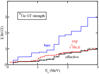
Figure 8: Running sums of the ⁷⁶Ge $B(p,n)$ strengths as a function of the excitation energy $E_{x}$ up to 3 MeV (see text for details).

This figure, as Table 4, evidences how crucial it is to take into account the renormalization of the GT operator to obtain a good agreement between theory and experiment. It is worth adding that the contribution of the blocking effect is almost unrelevant.

For the sake of completeness, we have calculated the theoretical total ${\rm GT}^{-}$ strengths, and obtained the values 18.2, 6.9, and 7.2 with the bare operator (I), and the effective ones (II) and (III), respectively.

III.3 ⁸²Se

As for ⁷⁶Ge and ⁷⁶Se, the shell model calculation for ⁸²Se and ⁸²Kr has been carried out using, as model space, the four proton and neutron orbitals $0f_{5/2}$, $1p_{3/2}$,$1p_{1/2}$ and $0g_{9/2}$ placed outside ⁵⁶Ni. In Fig. 9 the calculated low-energy spectra and $B(E2)$s are compared with experiment ens ; xun .

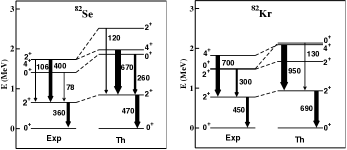
Figure 9: Same as in Fig. 5, but for ⁸²Se and ⁸²Kr (see text for details).

The agreement between theory and experiment can be considered satisfactory, the largest discrepancy, in both nuclei, occurring for the $B(E2;0^{+}_{2}\rightarrow 2^{+}_{1})$s, whose calculated values are about a factor 3 smaller than the observed ones.

As regards the observables linked to the $M1$ operator, the only available data for the low-lying states reported in Fig. 9 are the magnetic dipole moments shown in Table 5.

Table 5: Experimental and calculated magnetic dipole moments (in ${\rm nm}$) of ⁸²Se and ⁸²Kr. We report those for the observed states in Fig. 9.

Nucleus	$J$	$\mu_{\rm Expt}$	I	II	III
82Se
	$2^{+}_{1}$	$+0.99\pm 0.06$ ens	+0.72	+1.03	+1.05
	$4^{+}_{1}$	$2.3\pm 1.5$ ens	+1.17	+1.88	+1.93
82Kr
	$2^{+}_{1}$	$+0.80\pm 0.04$ ens	+0.50	+0.83	+0.83
	$4^{+}_{1}$	$+1.2\pm 0.8$ ens	+0.5	+1.3	+1.3

Since the model space is the same as for $A=76$ nuclei, the matrix elements of the effective $M1$ operator (II) are those reported in Table A.V. The action of the effective operators, as can be observed from the inspection of Table 5, is to improve the comparison with the data of the shell-model results, with respect to those obtained with the bare operator (I). This result evidences the role of the renormalization of the bare operator to take into account the degrees of freedom that have been left out by constraining the nuclear wave function to the valence nucleons interacting in the truncated model space.

As for the $2\nu\beta\beta$ decay of ⁷⁶Ge, the quenching of the matrix elements of the GT operator, shown in Table A.VIII, is crucial to improve our calculation of the NME of the decay of ⁸²Se into ⁸²Kr. In fact, the NME calculated with the bare operator overestimates the experimental value Barabash (2015) by a factor 4, as can be inferred from Table 6, while calculations performed with the effective operators (II-III) provide far better results.

Table 6: Same as in Table 2, but for the $2\nu\beta\beta$ decay of ⁸²Se (see text for details).

Decay	NMEExpt	I	II	III
82Se $\rightarrow$ 82Kr	$0.083\pm 0.004$	0.347	0.111	0.109

The quenching of the effective GT operator is a feature that is crucial also to provide a calculated $\Sigma B(p,n)$ curve for ⁸²Se, as a function of the excitation energy, that almost overlaps with the experimental one Frekers et al. (2016), as can be seen in Fig. 10 where the running sums of the ⁸²Se GT strengths up to a 3 MeV excitation energy are reported.

Figure 10: Running sums of the ⁸²Se $B(p,n)$ strengths as a function of the excitation energy $E_{x}$ up to 3 MeV (see text for details).

As for the calculations of ⁴⁸Ca, ⁷⁶Ge $\Sigma B(p,n)$, we observe a negligible role of the blocking effect.

We conclude this section reporting the calculated total ${\rm GT}^{-}$ strengths that are 21.6, 8.5, and 8.9 with the bare operator (I), and the effective ones (II) and (III), respectively.

III.4 ¹³⁰Te

The shell-model calculation for ¹³⁰Te and ¹³⁰Xe are performed within the model space spanned by the five proton and neutron orbitals $0g_{7/2}$, $1d_{5/2}$,$1d_{3/2}$, $2s_{1/2}$ and $0h_{11/2}$, considering ¹⁰⁰Sn as closed core. For the sake of completeness, the experimental ens ; xun and calculated low-energy spectra and $B(E2)$s, already reported in Ref. Coraggio et al. (2017), are also presented in this work in Fig. 11.

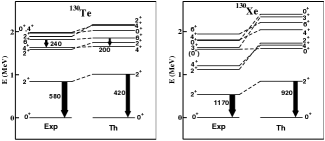
Figure 11: Same as in Fig. 5, but for ¹³⁰Te and ¹³⁰Xe (see text for details).

From inspection of Fig. 11, we observe that the comparison between the calculated and experimental low-energy spectra is very good for ¹³⁰Te, while is less satisfactory for ¹³⁰Xe. As regards the calculated $B(E2)$s, they compare well with the observed values for both nuclei, providing good expectations about the reliability of the SM wavefunctions.

In Table 7 the calculated $B(M1;2^{+}_{3}\rightarrow 2^{+}_{1})$ of ¹³⁰Te is reported and compared with the two experimental values of Ref. Hicks et al. (2008). In the same table the calculated and observed magnetic dipole moments of ¹³⁰Te and ¹³⁰Xe can be found.

Table 7: Same as in Table 1, but for ¹³⁰Te and ¹³⁰Xe (see text for details). We report those for the observed states in Fig. 11.

Nucleus	$J_{i}\rightarrow J_{f}$	$B(M1)_{\rm Expt}$	I	II	III
130Te
	$2^{+}_{3}\rightarrow 2^{+}_{1}$	$0.037^{+0.03}_{-0.04}$ Hicks et al. (2008)	0.057	0.085	0.077
		$0.097^{+0.08}_{-0.11}$ Hicks et al. (2008)
Nucleus	$J$	$\mu_{\rm Expt}$	I	II	III
130Te
	$2^{+}_{1}$	$0.58\pm 0.10$ ens	+0.52	+0.71	+0.71
130Xe
	$2^{+}_{1}$	$0.57\pm 0.14$ ens	+0.50	+0.67	+0.66

As can be seen, similarly to the results of the calculations for ⁷⁶Ge and ⁸²Se, the role of the effective $M1$ operator is relevant. As a matter of fact, the smaller $B(M1)$ values, compared with the one calculated with the bare operator, are a consequence of the general quenching of the non-diagonal matrix elements reported in Table A.VI. On the other side, the enhancement of the proton $0g_{7/2}$ diagonal matrix element is responsible for the larger dipole moments, when they are calculated employing the effective operators (II) and (III). Actually, because of the large experimental errors, it is not clear if the effective operators are able to provide a better agreement with experiment for the dipole moments with respect to the bare operator. As regards the $B(M1;2^{+}_{3}\rightarrow 2^{+}_{1})$, it turns out that our calculated values are closer to the smallest of the two values reported in Ref. Hicks et al. (2008). Finally, it is worth noting that there is no sizeable role of the blocking effect.

The calculated and experimental values of the NME for the ¹³⁰Te $2\nu\beta\beta$ decay Barabash (2015) are reported in Table 8.

Table 8: Same as in Table 2, but for the $2\nu\beta\beta$ decay (in MeV^-1) of ¹³⁰Te (see text for details).

Decay	NMEExpt	I	II	III
130Te $\rightarrow$ 130Xe	$0.031\pm 0.004$	0.131	0.057	0.061

As shown in our previous study Coraggio et al. (2017), where the matrix elements of the effective GT operator can be found in Tables (III-IV), the quenching of the bare operator (I) provided by the effective ones (II-III) plays a fundamental role to obtain a reasonable comparison with the experimental NME. As a matter of fact, our shell model calculation gives a $2\nu\beta\beta$ NME that is almost 4 times bigger than the experimental one, starting from GT operator (I). On the other hand, the effective operators, derived via many-body perturbation theory, take into account the reduction of the full Hilbert space to configurations constrained by the valence nucleons interacting in the model space and provide NMEs that are almost within experimental error bars.

These considerations hold, obvioulsy, also for the calculation of the ¹³⁰Te $\Sigma B(p,n)$, whose results are reported in Fig. 12 and compared with available data Puppe et al. (2012) up to 3 MeV excitation energy.

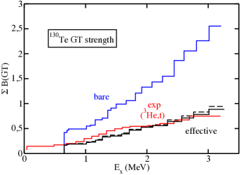
Figure 12: Running sums of the ¹³⁰Te $B(p,n)$ strengths as a function of the excitation energy $E_{x}$ up to 3 MeV (see text for details).

As for the ⁷⁶Ge and ⁸²Se running sums, the curves obtained with the effective operators (II-III) lie much closer to the experimental one than that calculated employing the bare operator (I), and almost overlap each other.

The total ${\rm GT}^{-}$ strengths, obtained with effective operators (I-III), are 46.4, 18.3, and 18.6, respectively.

III.5 ¹³⁶Xe

The shell-model calculations for ¹³⁶Xe and ¹³⁶Ba are carried out using the same model space, effective Hamiltonian and transition operators as for ¹³⁰Te and ¹³⁰Xe, and details about SP energies, TBMEs, effective charges, and effective GT matrix elements can be found in Ref. Coraggio et al. (2017).

We present, as in our previous study, the experimental ens ; xun and calculated low-energy spectra and $B(E2)$s which we have reported in Fig. 13.

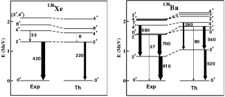
Figure 13: Same as in Fig. 5, but for ¹³⁶Xe and ¹³⁶Ba (see text for details).

The comparison between theory and experiment, as regards the low-lying excited states and the $B(E2)$ transition rates, is excellent for both nuclei, testifying once more the reliability of the realistic shell model.

In Table 9 we report the calculated and experimental $B(M1)$s of ¹³⁶Ba, involving some of the excited states reported in Fig. 13, together with the $J=2^{+}_{1}$ magnetic dipole moment. We compare also theory and experiment for the $J=2^{+}_{1},4^{+}_{1}$ magnetic dipole moments of ¹³⁶Xe.

Table 9: Same as in Table 1, but for ¹³⁶Xe and ¹³⁶Ba (see text for details). We report those for the observed states in Fig. 13.

Nucleus	$J_{i}\rightarrow J_{f}$	$B(M1)_{\rm Expt}$	I	II	III
136Ba
	$2^{+}_{2}\rightarrow 2^{+}_{1}$	$0.02\pm 0.1$ Mukhopadhyay et al. (2008)	0.07	0.06	0.06
	$2^{+}_{3}\rightarrow 2^{+}_{1}$	$0.002\pm 0.002$ Mukhopadhyay et al. (2008)	0.006	0.002	0.001
	$4^{+}_{2}\rightarrow 4^{+}_{1}$	$0.06^{+0.08}_{-0.05}$ Mukhopadhyay et al. (2008)	0.15	0.10	0.09
Nucleus	$J$	$\mu_{\rm Expt}$	I	II	III
136Xe
	$2^{+}_{1}$	$1.53\pm 0.09$ ens	+1.05	+1.15	+1.14
	$4^{+}_{1}$	$3.2\pm 0.6$ ens	+2.02	+2.24	+2.22
136Ba
	$2^{+}_{1}$	$0.69\pm 0.10$ ens	+0.48	+0.60	+0.59

As a matter of fact, we observe the same tendency we have found in the previous calculations, that is the quenching of $B(M1)$ values obtained with effective operators (II-III), and the enhancement of the dipole moments when the same operators are employed. This is grounded on the same observations we have made in Section III.4, and supported by the inspection of the list of the matrix elements in Table A.VI.

Actually, both features lead to an improvemement in the description of the data, and support again the crucial role of the renormalization of transition operators by way of the many-body perturbation theory.

This consideration is even more valid when we consider the calculation of the NME for the ¹³⁶Xe $2\nu\beta\beta$ decay, whose results are reported in Table 10 and compared with the datum Barabash (2015).

Table 10: Same as in Table 2, but for the $2\nu\beta\beta$ decay (in MeV^-1) of ¹³⁶Xe (see text for details).

Decay	NMEExpt	I	II	III
136Xe $\rightarrow$ 136Ba	$0.0181\pm 0.0007$	0.0910	0.0332	0.0341

We see that the (II-III) NMEs are more than a factor 3 smaller than the value obtained with the bare operator (I), and closer to the experimental value. The same feature comes out in Fig. 14, where we report the calculated and experimental Frekers et al. (2013) $\Sigma B(p,n)$ of ¹³⁶Xe up to 4.5 MeV excitation energy.

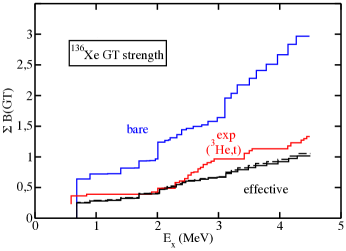
Figure 14: Running sums of the ¹³⁶Xe $B(p,n)$ strengths as a function of the excitation energy $E_{x}$ up to 4.5 MeV (see text for details).

Also for the ¹³⁶Xe running sums, the many-body renormalization of the GT operator is crucial to reproduce the experimental curve, with a negligible contribution of the blocking effect.

The total ${\rm GT}^{-}$ strengths, obtained with bare and effective operators (I-III), are 51.9, 20.7, and 21.0, respectively.

IV Conclusions and Outlook

In this paper we have studied the role of effective operators to calculate, within the realistic shell model, observables that are related to spin- and spin-isospin-dependent transitions. Our main focus has been on GT transitions for nuclei that are candidates for the detection of the $0\nu\beta\beta$-decay, and we have calculated, for several nuclei and over a wide mass range, $2\nu\beta\beta$-decay NMEs and the running sums of the $B(p,n)$ strengths to compare them with the available data. Since the magnetic-dipole $M1$ operator incorporates an isovector-spin term with the same structure of the GT operator, we have extended this analysis to the calculation of $B(M1)$s and magnetic dipole moments to strengthen our investigation.

As a matter of fact, our aim has been to demonstrate that the present status of the many-body perturbation theory allows to derive consistently effective Hamiltonians and transition operators that are able to reproduce quantitatively the observed spectroscopic and decay properties, without resorting to an empirical quenching of the axial coupling constant $g_{A}$, or to empirically fitted spin and orbital $g$-factors $g_{s},g_{l}$.

The quenching factors corresponding to the matrix eIements of the effective $M1$ and GT operators are reported in Tables A.IV-A.VI and Tables A.VII-A.IX, respectively. It is worth noting that the calculated quenching effect on the $M1$ operator is overall smaller than for GT transitions, which points to the fact that the two operators are differently affected by the renormalization procedure. This result highlights that for the renormalization of the $M1$ operator a non-negligible role is played by its isoscalar and isovector orbital components. As a matter of fact, from the inspection of these tables, the quenching of proton-proton $M1$ matrix elements is overall largely different from the $GT$ one, the latter being much closer to that obtained for neutron-neutron $M1$ matrix elements (which own the spin component only).

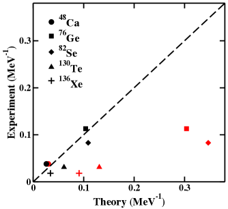
Figure 15: Correlation plot between the calculated (x-axis) and the experimental (y-axis) $2\nu\beta\beta$ decay NMEs (see text for details).

In order to show and stress pictorially the main outcome of our study about the relevance played by effective transition operators, in Fig. 15 we report a correlation plot between our calculated $2\nu\beta\beta$ decay NMEs and the corresponding experimental values. The quantities in Fig. 15 are already reported in Tables 2,4,6,8,10.

The red symbols correspond to the results obtained employing the bare operators (I), while the black ones indicate the results obtained with the effective operators (III).

As can be seen, the red points are all spread on the lower side of the figure, except the one corresponding to ⁴⁸Ca, and lie far away from the identity, that is represented by a dashed line. This feature characterizes the nuclei that are described by way of a model space where some of its orbitals lack their spin-orbit counterparts, leading to an overestimation of the calculated NME with respect to the experimental value.

The black points, that correspond to the effective GT operators, on the other hand regroup themselves close to the identity, as a reliable calculation should do.

It is worth reminding that our results may be traced back to earlier investigations carried out by Towner and collaborators since the 1980s (see for instance Towner and Khanna (1983); Towner (1987); Johnstone and Towner (1998); Brown et al. (2005)), where the role of microscopically derived effective spin-dependent operators is enlightened. Present work takes advantage of modern developments to derive the effective shell-model Hamiltonians and operators (see for example Refs. Coraggio et al. (2012); Suzuki and Okamoto (1995)), and up-to-date approaches to the renormalization of realistic $NN$ potentials Bogner et al. (2002).

On the above grounds, we intend to extend our study by investigating the role of meson-exchange corrections to the electroweak currents Park et al. (1993); Pastore et al. (2009); Piarulli et al. (2013); Baroni et al. (2016a). More precisely, we aim in a near future at building up effective shell-model Hamiltonians and operators starting from two- and three-body nuclear potentials derived within the framework of chiral perturbation theory Fukui et al. (2018), and taking also into account the contributions of chiral two-body electroweak currents to the effective GT operators. As a matter of fact, recent studies have shown that $\beta$- and neutrinoless double-beta decays may be significantly affected by these contributions Menéndez et al. (2011); Wang et al. (2018), when consistently starting from chiral potentials.

At last, our final goal is to benefit from the expertise we have gained to evaluate the $0\nu\beta\beta$ decay NMEs for the nuclei studied in present paper Coraggio et al. (2019).

*

Appendix A Tables of SP energies and effective operators

A.1 SP energies

Table A.I: Theoretical proton and neutron SP energy spacings (in MeV) for ⁴⁰Ca core.

	Proton SP spacings	Neutron SP spacings
$0f_{7/2}$	0.0	0.0
$0f_{5/2}$	8.6	7.8
$1p_{3/2}$	1.6	2.1
$1p_{1/2}$	3.3	4.0

Table A.II: Theoretical proton and neutron SP energy spacings (in MeV) for ⁵⁶Ni core.

	Proton SP spacings	Neutron SP spacings
$0f_{5/2}$	0.2	0.0
$1p_{3/2}$	0.0	0.5
$1p_{1/2}$	0.6	1.1
$0g_{9/2}$	3.1	3.5

Table A.III: Theoretical proton and neutron SP energy spacings (in MeV) for ¹⁰⁰Sn core.

	Proton SP spacings	Neutron SP spacings
$0g_{7/2}$	0.0	0.0
$1d_{5/2}$	0.3	0.6
$1d_{3/2}$	1.2	1.5
$2s_{1/2}$	1.1	1.2
$0h_{11/2}$	1.9	2.7

A.2 Effective $M1$ and GT operators

Table A.IV: Proton and neutron matrix elements of the effective magnetic dipole operator $M1$ (I) (in $\mu_{N}$) for the ⁴⁰Ca core. In the last column we report the corresponding quenching factors. For $l-$forbidden matrix elements there is no quenching factor to be shown.

$n_{a}l_{a}j_{a}~{}n_{b}l_{b}j_{b}$	$T_{z}$	$M1_{\rm eff}$	quenching factor
$0f_{7/2}~{}0f_{7/2}$	+1/2	8.760	0.965
$0f_{7/2}~{}0f_{5/2}$	+1/2	-3.986	0.961
$0f_{5/2}~{}0f_{7/2}$	+1/2	4.640	1.118
$0f_{5/2}~{}0f_{5/2}$	+1/2	1.310	1.073
$0f_{5/2}~{}1p_{3/2}$	+1/2	-0.017
$1p_{3/2}~{}0f_{5/2}$	+1/2	0.014
$1p_{3/2}~{}1p_{3/2}$	+1/2	4.462	0.933
$1p_{3/2}~{}1p_{1/2}$	+1/2	-2.396	0.926
$1p_{1/2}~{}1p_{3/2}$	+1/2	2.377	0.919
$1p_{1/2}~{}1p_{1/2}$	+1/2	-0.304	0.962
$0f_{7/2}~{}0f_{7/2}$	-1/2	-2.237	0.746
$0f_{7/2}~{}0f_{5/2}$	-1/2	3.308	0.956
$0f_{5/2}~{}0f_{7/2}$	-1/2	-3.582	1.035
$0f_{5/2}~{}0f_{5/2}$	-1/2	2.727	1.409
$0f_{5/2}~{}1p_{3/2}$	-1/2	-0.026
$1p_{3/2}~{}0f_{5/2}$	-1/2	0.024
$1p_{3/2}~{}1p_{3/2}$	-1/2	-2.074	0.859
$1p_{3/2}~{}1p_{1/2}$	-1/2	2.025	0.938
$1p_{1/2}~{}1p_{3/2}$	-1/2	-2.008	0.930
$1p_{1/2}~{}1p_{1/2}$	-1/2	0.799	1.047

Table A.V: Same as in Table A.IV, but for the ⁵⁶Ni core.

$n_{a}l_{a}j_{a}~{}n_{b}l_{b}j_{b}$	$T_{z}$	$M1_{\rm eff}$	quenching factor
$0f_{5/2}~{}0f_{5/2}$	+1/2	2.212	1.812
$0f_{5/2}~{}1p_{3/2}$	+1/2	-0.033
$1p_{3/2}~{}0f_{5/2}$	+1/2	0.026
$1p_{3/2}~{}1p_{3/2}$	+1/2	3.358	0.739
$1p_{3/2}~{}1p_{1/2}$	+1/2	-1.554	0.601
$1p_{1/2}~{}1p_{3/2}$	+1/2	1.586	0.613
$1p_{1/2}~{}1p_{1/2}$	+1/2	-0.091	0.288
$0g_{9/2}~{}0g_{9/2}$	+1/2	10.174	0.877
$0f_{5/2}~{}0f_{5/2}$	-1/2	1.338	0.691
$0f_{5/2}~{}1p_{3/2}$	-1/2	-0.024
$1p_{3/2}~{}0f_{5/2}$	-1/2	0.028
$1p_{3/2}~{}1p_{3/2}$	-1/2	-1.233	0.511
$1p_{3/2}~{}1p_{1/2}$	-1/2	1.178	0.546
$1p_{1/2}~{}1p_{3/2}$	-1/2	-1.209	0.560
$1p_{1/2}~{}1p_{1/2}$	-1/2	0.512	0.671
$0g_{9/2}~{}0g_{9/2}$	-1/2	-0.473	0.145

Table A.VI: Same as in Table A.IV, but for the ¹⁰⁰Sn core.

$n_{a}l_{a}j_{a}~{}n_{b}l_{b}j_{b}$	$T_{z}$	$M1_{\rm eff}$	quenching factor
$0g_{7/2}~{}0g_{7/2}$	+1/2	3.013	1.120
$0g_{7/2}~{}1d_{5/2}$	+1/2	-0.064
$1d_{5/2}~{}0g_{7/2}$	+1/2	0.060
$1d_{5/2}~{}1d_{5/2}$	+1/2	5.190	0.765
$1d_{5/2}~{}1d_{3/2}$	+1/2	-2.180	0.628
$1d_{3/2}~{}1d_{5/2}$	+1/2	2.274	0.655
$1d_{3/2}~{}1d_{3/2}$	+1/2	0.407	2.599
$1d_{3/2}~{}2s_{1/2}$	+1/2	-0.123
$2s_{1/2}~{}1d_{3/2}$	+1/2	0.119
$2s_{1/2}~{}2s_{1/2}$	+1/2	2.453	0.734
$0h_{11/2}~{}0h_{11/2}$	+1/2	12.349	0.861
$0g_{7/2}~{}0g_{7/2}$	-1/2	1.984	0.851
$0g_{7/2}~{}1d_{5/2}$	-1/2	-0.008
$1d_{5/2}~{}0g_{7/2}$	-1/2	0.008
$1d_{5/2}~{}1d_{5/2}$	-1/2	-1.417	0.523
$1d_{5/2}~{}1d_{3/2}$	-1/2	1.681	0.580
$1d_{3/2}~{}1d_{5/2}$	-1/2	-1.756	0.606
$1d_{3/2}~{}1d_{3/2}$	-1/2	1.081	0.746
$1d_{3/2}~{}2s_{1/2}$	-1/2	0.076
$2s_{1/2}~{}1d_{3/2}$	-1/2	-0.071
$2s_{1/2}~{}2s_{1/2}$	-1/2	-1.414	0.618
$0h_{11/2}~{}0h_{11/2}$	-1/2	-0.696	0.198

Table A.VII: Matrix elements of the proton-neutron effective GT⁺ and GT^- operators for the ⁴⁰Ca core. In the last two columns we report the corresponding quenching factors of present work (I) and those reported in the work of Ref. Siiskonen et al. (2001) (see text for details). For $l-$forbidden matrix elements there is no quenching factor to be shown.

$n_{a}l_{a}j_{a}~{}n_{b}l_{b}j_{b}$	GT${}^{-}_{\rm eff}$	quenching factor
$0f_{7/2}~{}0f_{7/2}$	2.870	0.995
$0f_{7/2}~{}0f_{5/2}$	-3.210	0.964
$0f_{5/2}~{}0f_{7/2}$	3.941	1.183
$0f_{5/2}~{}0f_{5/2}$	-2.104	1.130
$0f_{5/2}~{}1p_{3/2}$	-0.033
$1p_{3/2}~{}0f_{5/2}$	0.001
$1p_{3/2}~{}1p_{3/2}$	2.162	0.931
$1p_{3/2}~{}1p_{1/2}$	-1.906	0.918
$1p_{1/2}~{}1p_{3/2}$	1.901	0.915
$1p_{1/2}~{}1p_{1/2}$	-0.691	0.953
$n_{a}l_{a}j_{a}~{}n_{b}l_{b}j_{b}$	GT${}^{+}_{\rm eff}$	quenching factor (I)	quenching factor (II)
$0f_{7/2}~{}0f_{7/2}$	2.706	0.938	0.905
$0f_{7/2}~{}0f_{5/2}$	-3.012	0.904	0.856
$0f_{5/2}~{}0f_{7/2}$	3.276	0.984
$0f_{5/2}~{}0f_{5/2}$	-1.737	0.932	0.882
$0f_{5/2}~{}1p_{3/2}$	-0.001
$1p_{3/2}~{}0f_{5/2}$	0.026
$1p_{3/2}~{}1p_{3/2}$	2.135	0.921	0.880
$1p_{3/2}~{}1p_{1/2}$	-1.879	0.904	0.863
$1p_{1/2}~{}1p_{3/2}$	1.871	0.901
$1p_{1/2}~{}1p_{1/2}$	-0.686	0.935	0.932

Table A.VIII: Same as in Table A.VII, but for the ⁵⁶Ni core.

$n_{a}l_{a}j_{a}~{}n_{b}l_{b}j_{b}$	GT${}^{-}_{\rm eff}$	quenching factor
$0f_{5/2}~{}0f_{5/2}$	-0.674	0.362
$0f_{5/2}~{}1p_{3/2}$	-0.085
$1p_{3/2}~{}0f_{5/2}$	0.006
$1p_{3/2}~{}1p_{3/2}$	1.441	0.620
$1p_{3/2}~{}1p_{1/2}$	-1.141	0.549
$1p_{1/2}~{}1p_{3/2}$	1.189	0.572
$1p_{1/2}~{}1p_{1/2}$	-0.482	0.657
$0g_{9/2}~{}0g_{9/2}$	1.608	0.511
$n_{a}l_{a}j_{a}~{}n_{b}l_{b}j_{b}$	GT${}^{+}_{\rm eff}$	quenching factor (I)	quenching factor (II)
$0f_{5/2}~{}0f_{5/2}$	-0.638	0.342	0.458
$0f_{5/2}~{}1p_{3/2}$	-0.011
$1p_{3/2}~{}0f_{5/2}$	0.061
$1p_{3/2}~{}1p_{3/2}$	1.405	0.605	0.689
$1p_{3/2}~{}1p_{1/2}$	-1.159	0.558	0.680
$1p_{1/2}~{}1p_{3/2}$	1.121	0.539
$1p_{1/2}~{}1p_{1/2}$	-0.468	0.638
$0g_{9/2}~{}0g_{9/2}$	1.536	0.488	0.802

Table A.IX: Same as in Table A.VII, but for the ¹⁰⁰Sn core.

$n_{a}l_{a}j_{a}~{}n_{b}l_{b}j_{b}$	GT${}^{-}_{\rm eff}$	quenching factor
$0g_{7/2}~{}0g_{7/2}$	-1.168	0.521
$0g_{7/2}~{}1d_{5/2}$	-0.108
$1d_{5/2}~{}0g_{7/2}$	0.000
$1d_{5/2}~{}1d_{5/2}$	1.686	0.647
$1d_{5/2}~{}1d_{3/2}$	-1.525	0.547
$1d_{3/2}~{}1d_{5/2}$	1.708	0.613
$1d_{3/2}~{}1d_{3/2}$	-0.888	0.638
$1d_{3/2}~{}2s_{1/2}$	-0.124
$2s_{1/2}~{}1d_{3/2}$	0.093
$2s_{1/2}~{}2s_{1/2}$	1.405	0.638
$0h_{11/2}~{}0h_{11/2}$	1.931	0.570
$n_{a}l_{a}j_{a}~{}n_{b}l_{b}j_{b}$	GT${}^{+}_{\rm eff}$	quenching factor (I)	quenching factor (II)
$0g_{7/2}~{}0g_{7/2}$	-1.168	0.521	0.472
$0g_{7/2}~{}1d_{5/2}$	0.001
$1d_{5/2}~{}0g_{7/2}$	0.102
$1d_{5/2}~{}1d_{5/2}$	1.686	0.647	0.595
$1d_{5/2}~{}1d_{3/2}$	-1.688	0.606	0.513
$1d_{3/2}~{}1d_{5/2}$	1.543	0.553
$1d_{3/2}~{}1d_{3/2}$	-0.888	0.638	0.652
$1d_{3/2}~{}2s_{1/2}$	-0.098
$2s_{1/2}~{}1d_{3/2}$	0.117
$2s_{1/2}~{}2s_{1/2}$	1.405	0.638
$0h_{11/2}~{}0h_{11/2}$	1.931	0.570

References

- Hjorth-Jensen et al. (2017) M. Hjorth-Jensen, M. P. Lombardo, and U. van Kolck, eds., Lecture Notes in Physics, vol. 936 (Springer, 2017).
- Hjorth-Jensen et al. (1995) M. Hjorth-Jensen, T. T. S. Kuo, and E. Osnes, Phys. Rep. 261, 125 (1995).
- Coraggio et al. (2012) L. Coraggio, A. Covello, A. Gargano, N. Itaco, and T. T. S. Kuo, Ann. Phys. 327, 2125 (2012).
- Coraggio et al. (2009) L. Coraggio, A. Covello, A. Gargano, N. Itaco, and T. T. S. Kuo, Prog. Part. Nucl. Phys. 62, 135 (2009).
- Ellis and Osnes (1977) P. J. Ellis and E. Osnes, Rev. Mod. Phys. 49, 777 (1977).
- Suzuki and Okamoto (1995) K. Suzuki and R. Okamoto, Prog. Theor. Phys. 93, 905 (1995).
- Siiskonen et al. (2001) T. Siiskonen, M. Hjorth-Jensen, and J. Suhonen, Phys. Rev. C 63, 055501 (2001).
- Holt and Engel (2013) J. D. Holt and J. Engel, Phys. Rev. C 87, 064315 (2013).
- Barea and Iachello (2009) J. Barea and F. Iachello, Phys. Rev. C 79, 044301 (2009).
- Barea et al. (2012) J. Barea, J. Kotila, and F. Iachello, Phys. Rev. Lett. 109, 042501 (2012).
- Barea et al. (2013) J. Barea, J. Kotila, and F. Iachello, Phys. Rev. C 87, 014315 (2013).
- Šimkovic et al. (2008) F. Šimkovic, A. Faessler, V. Rodin, P. Vogel, and J. Engel, Phys. Rev. C 77, 045503 (2008).
- Šimkovic et al. (2009) F. Šimkovic, A. Faessler, H. Müther, V. Rodin, and M. Stauf, Phys. Rev. C 79, 055501 (2009).
- Fang et al. (2011) D.-L. Fang, A. Faessler, V. Rodin, and F. Šimkovic, Phys. Rev. C 83, 034320 (2011).
- Faessler et al. (2012) A. Faessler, V. Rodin, and F. Simkovic, J. Phys. G 39, 124006 (2012).
- Šimkovic et al. (2018) F. Šimkovic, A. Smetana, and P. Vogel, Phys. Rev. C 98, 064325 (2018).
- Caurier et al. (2008) E. Caurier, F. Nowacki, and A. Poves, Eur. Phys. J. A 36, 195 (2008).
- Menéndez et al. (2009a) J. Menéndez, A. Poves, E. Caurier, and F. Nowacki, Phys. Rev. C 80, 048501 (2009a).
- Menéndez et al. (2009b) J. Menéndez, A. Poves, E. Caurier, and F. Nowacki, Nucl. Phys. A 818, 139 (2009b).
- Caurier et al. (2012) E. Caurier, F. Nowacki, and A. Poves, Phys. Lett. B 711, 62 (2012).
- Horoi et al. (2007) M. Horoi, S. Stoica, and B. A. Brown, Phys. Rev. C 75, 034303 (2007).
- Horoi (2013a) M. Horoi, Phys. Rev. C 87, 014320 (2013a).
- Horoi and Brown (2013) M. Horoi and B. A. Brown, Phys. Rev. Lett. 110, 222502 (2013).
- Neacsu and Horoi (2015) A. Neacsu and M. Horoi, Phys. Rev. C 91, 024309 (2015).
- Brown et al. (2015) B. A. Brown, D. L. Fang, and M. Horoi, Phys. Rev. C 92, 041301 (2015).
- Iwata et al. (2016) Y. Iwata, N. Shimizu, T. Otsuka, Y. Utsuno, J. Menéndez, M. Honma, and T. Abe, Phys. Rev. Lett. 116, 112502 (2016).
- Suhonen (2017a) J. Suhonen, Front. Phys. 5:55 (2017a).
- Park et al. (1993) T. S. Park, D. P. Min, and M. Rho, Phys. Rep. 233, 341 (1993).
- Pastore et al. (2009) S. Pastore, L. Girlanda, R. Schiavilla, M. Viviani, and R. B. Wiringa, Phys. Rev. C 80, 034004 (2009).
- Piarulli et al. (2013) M. Piarulli, L. Girlanda, L. E. Marcucci, S. Pastore, R. Schiavilla, and M. Viviani, Phys. Rev. C 87, 014006 (2013).
- Baroni et al. (2016a) A. Baroni, L. Girlanda, S. Pastore, R. Schiavilla, and M. Viviani, Phys. Rev. C 93, 015501 (2016a).
- Tanabashi et al. (2018) M. Tanabashi, K. Hagiwara, K. Hikasa, K. Nakamura, Y. Sumino, F. Takahashi, J. Tanaka, K. Agashe, G. Aielli, C. Amsler, et al. (Particle Data Group), Phys. Rev. D 98, 030001 (2018).
- Towner (1987) I. S. Towner, Phys. Rep. 155, 263 (1987).
- Towner and Khanna (1983) I. S. Towner and K. F. C. Khanna, Nucl. Phys. A 399, 334 (1983).
- Suhonen (2017b) J. Suhonen, Phys. Rev. C 96, 055501 (2017b).
- Baroni et al. (2016b) A. Baroni, L. Girlanda, A. Kievsky, L. E. Marcucci, R. Schiavilla, and M. Viviani, Phys. Rev. C 94, 024003 (2016b).
- Kuo et al. (1981) T. T. S. Kuo, J. Shurpin, K. C. Tam, E. Osnes, and P. J. Ellis, Ann. Phys. (NY) 132, 237 (1981).
- Coraggio et al. (2017) L. Coraggio, L. De Angelis, T. Fukui, A. Gargano, and N. Itaco, Phys. Rev. C 95, 064324 (2017).
- Machleidt (2001) R. Machleidt, Phys. Rev. C 63, 024001 (2001).
- Bogner et al. (2001) S. Bogner, T. T. S. Kuo, and L. Coraggio, Nucl. Phys. A 684, 432c (2001).
- Bogner et al. (2002) S. Bogner, T. T. S. Kuo, L. Coraggio, A. Covello, and N. Itaco, Phys. Rev. C 65, 051301(R) (2002).
- Coraggio et al. (2015a) L. Coraggio, A. Covello, A. Gargano, N. Itaco, and T. T. S. Kuo, Phys. Rev. C 91, 041301 (2015a).
- Coraggio et al. (2015b) L. Coraggio, A. Gargano, and N. Itaco, JPS Conf. Proc. 6, 020046 (2015b).
- Coraggio et al. (2016) L. Coraggio, A. Gargano, and N. Itaco, Phys. Rev. C 93, 064328 (2016).
- Kuo and Osnes (1990) T. T. S. Kuo and E. Osnes, Lecture Notes in Physics, vol. 364 (Springer-Verlag, Berlin, 1990).
- Kuo et al. (1995) T. T. S. Kuo, F. Krmpotić, K. Suzuki, and R. Okamoto, Nucl. Phys. A 582, 205 (1995).
- Kuo et al. (1971) T. T. S. Kuo, S. Y. Lee, and K. F. Ratcliff, Nucl. Phys. A 176, 65 (1971).
- Coraggio et al. (2010) L. Coraggio, A. Covello, A. Gargano, and N. Itaco, Phys. Rev. C 81, 064303 (2010).
- Brandow (1967) B. H. Brandow, Rev. Mod. Phys. 39, 771 (1967).
- Krenciglowa and Kuo (1974) E. M. Krenciglowa and T. T. S. Kuo, Nucl. Phys. A 235, 171 (1974).
- (51) See Supplemental material at [URL will be inserted by publisher] for the list of two-body matrix elements of the shell-model hamiltonian .
- Coraggio et al. (2018) L. Coraggio, L. De Angelis, T. Fukui, A. Gargano, and N. Itaco, J. Phys. Conf. Ser. 1056, 012012 (2018).
- Baker and Gammel (1970) G. A. Baker and J. L. Gammel, The Padé Approximant in Theoretical Physics, vol. 71 of Mathematics in Science and Engineering (Academic Press, New York, 1970).
- Hoffmann et al. (1976) H. M. Hoffmann, Y. Starkand, and M. W. Kirson, Nucl. Phys. A 266, 138 (1976).
- Goodman et al. (1980) C. D. Goodman, C. A. Goulding, M. B. Greenfield, J. Rapaport, D. E. Bainum, C. C. Foster, W. G. Love, and F. Petrovich, Phys. Rev. Lett. 44, 1755 (1980).
- Taddeucci et al. (1987) T. N. Taddeucci, C. A. Goulding, T. A. Carey, R. C. Byrd, C. D. Goodman, C. Gaarde, J. Larsen, D. Horen, J. Rapaport, and E. Sugarbaker, Nucl. Phys. A 469, 125 (1987).
- Caurier et al. (2005) E. Caurier, G. Martínez-Pinedo, F. Nowacki, A. Poves, and A. P. Zuker, Rev. Mod. Phys. 77, 427 (2005).
- Haxton and Stephenson Jr. (1984) W. C. Haxton and G. J. Stephenson Jr., Prog. Part. Nucl. Phys. 12, 409 (1984).
- Sen’kov and Horoi (2013) R. A. Sen’kov and M. Horoi, Phys. Rev. C 88, 064312 (2013).
- Horoi (2013b) M. Horoi, J. Phys. Conf. Ser. 413, 012020 (2013b).
- Barabash (2015) A. S. Barabash, Nucl. Phys. A 935, 52 (2015).
- (62) Data extracted using the NNDC On-line Data Service from the ENSDF database, file revised as of November 6, 2018., URL https://www.nndc.bnl.gov/ensdf.
- (63) Data extracted using the NNDC On-line Data Service from the XUNDL database, file revised as of November 6, 2018., URL https://www.nndc.bnl.gov/ensdf/ensdf/xundl.jsp.
- Vanhoy et al. (1992) J. R. Vanhoy, M. T. McEllistrem, S. F. Hicks, R. A. Gatenby, E. M. Baum, E. L. Johnson, G. Molnár, and S. W. Yates, Phys. Rev. C 45, 1628 (1992).
- Yako et al. (2009) K. Yako, M. Sasano, K. Miki, H. Sakai, M. Dozono, D. Frekers, M. B. Greenfield, K. Hatanaka, E. Ihara, M. Kato, et al., Phys. Rev. Lett. 103, 012503 (2009).