Double parton scattering and the proton transverse structure at the LHC

Abstract

We consider double parton distribution functions (dPDFs), essential quantities in double parton scattering (DPS) studies, which encode novel non perturbative insight on the partonic proton structure. We develop the formalism to extract this information from dPDFs and present results by using constituent quark model calculations within the Light-Front approach, focusing on radiatively generated gluon dPDFs. Moreover, we generalize the relation between the mean transverse partonic distance between two active partons in a DPS process and the so called $\sigma_{eff}$ to include partonic correlations and the so called 2v1 mechanism contribution. Finally we investigate the impact of relativistic effects on digluon distributions and study the structure of the corresponding longitudinal and transverse correlations.

1 Introduction

A proper description of the event structure in hadronic collisions requires the inclusion of the so called multiple parton interactions (MPI) which affect both the multiplicity and structure of the hadronic final state [1, 2]. The Large Hadron Collider operation renewed the interest in MPI given the continuous demand for an increasingly detailed description of the hadronic final state which is crucial in many New Physics searches. In this rapidly evolving context, these type of studies have also received attention for their own sake since they might be sensitive to double partonic correlations in the colliding hadrons, see recent review in Ref. [3]. The simplest MPI process is the double parton scattering (DPS) [4, 5]. In such a process, a large momentum transfer is involved in both scatterings which enables the use of perturbative techniques to calculate the corresponding cross section. The latter depends on two-body quantities, the so called double Parton Distribution Functions (dPDFs), which are interpreted as the number densities of parton pair at a given transverse distance, $b_{\perp}$, and carrying longitudinal momentum fractions ($x_{1},x_{2}$) of the parent proton [1, 6, 7]. Double PDFs are not perturbatively calculable from first principles, a feature shared with usual PDFs and other quantities in QCD. Moreover, due to their dependence upon the partonic interdistance [7], they contain information on the hadronic structure complementary to those obtained from one-body distributions such as generalized parton distribution functions (GPDs) and transverse momentum dependent PDFs (TMDs). Unfortunately the DPS cross section is obtained by integrating dPDFs over $b_{\perp}$ so that such a dependence is not directly measurable [1]. In this scenario, hadronic models have been used to obtain basic information on dPDFs and to gauge the phenomenological impact of longitudinal and transverse correlations, see Refs. [8, 9, 10, 11, 12, 13], along with spin correlations [11, 14, 15, 16, 17]. We mention that quantities related to dPDFs, and encoding double parton correlations, have been recently calculated for pion by means of Lattice techniques [18]. Despite the wealth of information encoded in dPDFs, present experimental knowledge on DPS cross section is accumulated, up to now, into the so called effective cross section, $\sigma_{eff}$, for recent results see e.g. Refs. [19, 20, 21, 22, 23, 24]. The latter is defined through the ratio of the product of two single parton scattering cross sections to the DPS cross section with the same final states. In the present paper, we continue the investigation of the relationship between $\sigma_{eff}$ and the mean interpartonic distance pursued in Ref. [25]. We study its modification induced by including the so called splitting 2v1 term contribution in DPS processes [26, 27, 28, 29, 30, 31, 32, 33, 34, 35] and, separately, the effects of longitudinal correlations in dPDFs. Numerical estimates will be shown and discussed in the kinematics of DPS processes initiated by digluon distributions, see e.g. Refs. [36, 37, 40, 39, 38] on this topic, which are perhaps the most interesting distributions in the DPS context. Such distributions are radiatively generated by pQCD evolution [6, 26, 27, 28, 32, 33, 34, 35, 41, 42, 43, 44, 45] starting from valence dPDF model calculation at the hadronic scale, $Q_{0}$. The digluon distrubution, in principle, is likely to have a non perturbative contribution at $Q_{0}$. In the present work, we make use of a pure radiative evolution scheme, and therefore it is our precise choice to neglect such an additional input which requires the modelization of the non perturbative sea quarks and gluons distributions, such those proposed in Ref. [46]. On the other hand it must be emphasized that in case of ordinary DIS structure functions measurements, predictions based on parton distributions evolved in such a scheme are not able to reproduce the small $x$ behaviour of the data and a non perturbative sea quarks and gluon PDFs input are required. Moreover, in such a radiative scheme and given the structure of dPDFs evolution equations, digluon interdistance follows the pattern of that of valence quarks obtained from the underlying hadronic model used for the dPDF calculations. DPS measurements, sensitive to gluon initiated processes, will then provide a test of our approach. In the last part of the paper, we focus on relativistic effects in dPDF model calculations, in the relevant kinematic conditions of collider experiments, and already addressed in Ref. [12] for valence quarks at the hadronic scale. The aim of this part of the analysis is to offer insight to unfactorized ansatz for dPDFs as induced by the implementation of relativistic effects in dPDFs calculation via Melosh operators.

The paper is organized as follows. In Sec. 2 we will discuss processes and corresponding kinematic conditions which we will focus upon in this analysis. In Sec. 3 we describe the formalism which allows to obtain physical information on the proton structure from dPDFs. In Sec. 4 we introduce the so called $\sigma_{eff}$, relevant quantity in DPS analyses and show how the latter is related to the geometrical properties of the proton. In Sec. 5 we discuss relativistic effects in dPDF calculations and then present our Conclusions.

2 Analysis strategy and calculation details

In the present analysis we will focus on the digluon distributions and therefore we consider DPS prototype processes:

$$pp\rightarrow J/\Psi J/\Psi X,\;\;\;pp\rightarrow HHX\;,$$ (1)

for which the production mechanism is dominated by gluons and where each final state particle is produced in a distinct parton-parton scattering. Double $J/\Psi$ production has been already measured both at Tevatron and LHC [20, 23, 24, 47, 48]. Double Higgs production via DPS has been studied in the literature [30], but not yet measured given its rather low cross section. We mention here that it would be also interesting to consider the mixed process $pp\rightarrow HJ/\Psi X$ with final state produced via DPS which, to the best of our knowledge, has never been considered in the literature. We also mention that interesting information could be gained from the comparison of the double $J/\Psi$ production with the double open charm one in the same kinematics. The combined measurements of these DPS processes, among many others with a less pure gluonic initial state but larger cross sections, give a wide coverage of digluon distribution both in hard scale and fractional momenta. We define the partonic subprocess in the two scatterings in Eq. (1) as

$$p_{i}(k_{1})+p_{k}(k_{3})\rightarrow A(k_{A})X\;\;\mbox{and}\;\;p_{j}(k_{2})+p_{l}(k_{4})\rightarrow B(k_{B})X,\;\;\mbox{with}\;\;A,B=J/\Psi,H\,,$$ (2)

where $p$’s and $k$’s are the relevant parton flavour and momenta, respectively. Since heavy particles appearing in Eq. (1) are produced by partonic annihilation in lowest order of perturbation theory, the fractional momenta of the incident gluons can be reconstructed from the mass $m$, transverse momentum $k_{T}$ and rapidity $y$ of final state particles as

$$x_{1,3}=\frac{\sqrt{m_{A}^{2}+k_{T,A}^{2}}}{\sqrt{s}}e^{\pm y_{A}},\;\;\;x_{2,4}=\frac{\sqrt{m_{B}^{2}+k_{T,B}^{2}}}{\sqrt{s}}e^{\pm y_{B}}\,.$$ (3)

In our calculations we set the centre-of-mass energy to its nominal value at the LHC, $\sqrt{s}$=13 TeV, and consider two rapidity region: the central one covered by ATLAS and CMS, $|y|<1.2$ and the forward one covered by LHCb, $2<y<4.5$. Neglecting transverse momentum, $J/\Psi$ production gives access to fractional momenta in the range $10^{-6}\lesssim x\lesssim 10^{-2}$ while Higgs production in the range $10^{-4}\lesssim x\lesssim 1$. The factorization scale in each process is set equal to the mass of the particle, either the $J/\Psi$ or Higgs boson, produced in the final state, $\mu_{F,A}=m_{A}$ and $\mu_{F,B}=m_{B}$ with $m_{J/\Psi}=2m_{c}$. The differential DPS cross section, assuming that the two hard scatterings can be factorized [6, 28, 41, 49, 50, 51], involves dPDFs through an integral over the transverse partonic distance $b_{\perp}$ and reads [1, 6]:

$$d\sigma_{DPS}^{A+B}=\frac{m}{2}\int d^{2}b_{\perp}d\hat{\sigma}_{ik}^{A}\;d\hat{\sigma}_{jl}^{B}\;\tilde{F}_{ij}(x_{1},x_{2},b_{\perp})\tilde{F}_{kl}(x_{3},x_{4},b_{\perp})\,.$$ (4)

In Eq. (4) $d\hat{\sigma}$ are the differential partonic cross sections for processes with final state A or B respectively and the symmetry factor reads $m=1$ if $A=B$ and $m=2$ otherwise. Double PDFs appearing in Eq. (4), are multidimensional distributions encoding non perturbative features of the proton structure and are therefore complicated to model. Some guidance in building appropriate initial conditions is offered by physical intuition at small $x$ [6, 28, 29, 41, 44, 52] and by sum rules [29, 37, 38, 53]. Nevertheless, a large freedom is left in the gluon transverse spectrum, which is perhaps one of the most intriguing aspect for hadronic studies. In order to investigate some of these features, in the present paper we make use of dPDF calculations within constituent quark models (CQMs), e.g. Refs. [8, 9, 10, 11]. Following the line of Ref. [12], we have adopted the hypercentral quark model (HP), in its relativistic version [54] and, in order to highlight model independent effects on dPDFs, the harmonic oscillator model (HO) [55]. In particular, for the latter, we considered the version described in Ref. [12], where the model parameter $\alpha$, representing the width of the Gaussian, is set to be $\alpha^{2}=25$ fm^-2 in order to mimic a relativistic structure. These models differ from each other in many dynamical aspects and offer a parametrization of the only non-vanishing valence-valance dPDF at the hadronic scale, $Q_{0}$. All other distributions are then radiatively obtained at higher scales by performing pQCD evolution in its homogeneous form, which is appropriate at fixed $b_{\perp}$ [6, 44, 56]. The value of the hadronic scale $Q_{0}$ has been fixed according to the procedure outlined in Ref. [57], i.e. by tuning its value in order to reproduce known SPS cross sections by using single PDFs obtained by the same hadronic model and evolved starting from $Q_{0}$. The obtained value is given by $Q_{0}^{2}=0.26$ Ge$\mbox{V}^{2}$. Since both single and double PDFs are built upon the same hadronic model, $Q_{0}$ is used also as starting scale for dPDFs evolution. Since $Q_{0}$ is located in the infrared region, both distributions show a large sensitivity to its precise value. In order to reduce the impact of this choice on our results, we will often consider appropriate ratios involving single and double PDFs which decrease, and in many cases almost cancel, this dependence. This feature is particularly relevant for the calculation of the effective cross section which we will be introduced in the next Section.

3 Proton transverse structure from dPDFs

In this section we present the general formalism necessary to extract physical information on the proton structure from dPDFs, i.e. the mean partonic distance between two partons in the transverse plane. These results are completely general and do not require any specific assumption on dPDFs. Since the latter represent the number density of two parton with longitudinal momentum fractions $x_{1}$ and $x_{2}$ at a given transverse distance $b_{\perp}$ [1], they provide a new tool to access the 3D structure of the proton, complementary to that obtained from generalized parton distribution functions (GPDs). In particular, these two-body functions are sensitive to double parton correlations [3, 8, 9, 10, 11, 12, 13, 14, 18, 35, 36, 44, 45, 46] that can not be accessed by means of one-body distributions such as GPDs. To this aim we first introduce the effective form factor (EFF) [58, 25] as discussed in Ref. [25], i.e. by means of the hadron wave function $\Psi$ in the non relativistic limit:

$$f_{ij}(k_{\perp})=\int d\vec{k}_{1}d\vec{k}_{2}~{}\Psi^{\dagger}(\vec{k}_{1}+\vec{k}_{\perp},\vec{k}_{2})\tau_{i}\tau_{j}\Psi(\vec{k}_{1},\vec{k}_{2}+\vec{k}_{\perp})~{},$$ (5)

where $\vec{k}_{i}$ is the total momentum of the parton $i$ and $\tau_{i}$ the standard flavor projector. As discussed in Ref. [25], $k_{\perp}$ represents a transverse momentum imbalance between two partons in the amplitude and its conjugate [28]. The EFF represents the Fourier Transform of the number distribution of two partons at a given transverse distance [25, 58]:

$$f_{ij}(k_{\perp})=\int d^{2}b_{\perp}~{}e^{\vec{k}_{\perp}\cdot\vec{b}_{\perp}}\tilde{f}_{ij}(b_{\perp}).$$ (6)

This distribution can be written in terms of dPDFs in coordinate space, i.e. $\tilde{F}_{ij}(x_{1},x_{2},b_{\perp})$:

$$\tilde{f}_{ij}(b_{\perp})=\int dx_{1}~{}dx_{2}~{}\tilde{F}_{ij}(x_{1},x_{2},b_{\perp})~{}.$$ (7)

$\tilde{F}_{ij}(x_{1},x_{2},b_{\perp})$ encode information on the proton structure such as correlations between the longitudinal momentum fractions of two partons and their partonic distance. The latter, for a pair of partons with flavour $i$ and $j$ and fractional momenta $x_{1}$ and $x_{2}$, is defined as

$$\langle b_{\perp}^{2}\rangle^{ij}_{x_{1},x_{2}} =\frac{\displaystyle\int d^{2}b_{\perp}~{}b^{2}_{\perp}\tilde{F}_{ij}(x_{1},x_{2},b_{\perp},Q^{2})}{\displaystyle\int d^{2}b_{\perp}~{}\tilde{F}_{ij}(x_{1},x_{2},b_{\perp},Q^{2})}~{},$$ (8)

where $Q^{2}$ is a generic hard scale at which dPDFs are evaluated and we have denoted $b_{\perp}\equiv|\vec{b}_{\perp}|$. It is easy then to show that the mean partonic distance averaged over parton fractional momenta is given by

$$\langle b_{\perp}^{2}\rangle^{ij}=\frac{\displaystyle\int d^{2}b_{\perp}~{}b_{\perp}^{2}\tilde{f}_{ij}(b_{\perp})}{\displaystyle\int d^{2}b_{\perp}~{}\tilde{f}_{ij}(b_{\perp})}~{}.$$ (9)

The above quantities can be related to each other as follows:

$$\langle b_{\perp}^{2}\rangle^{ij} =\int dx_{1}~{}dx_{2}~{}\langle b_{\perp}^{2}\rangle_{x_{1},x_{2}}^{ij}P_{ij}(x_{1},x_{2})~{},$$ (10)

where $P_{ij}(x_{1},x_{2})$ represents the probability of finding a pair of partons with flavours $i,j$ and longitudinal momentum fractions $x_{1},x_{2}$:

$$P_{ij}(x_{1},x_{2})=\frac{\displaystyle\int d^{2}b_{\perp}~{}\tilde{F}_{ij}(x_{1},x_{2},b_{\perp})}{\displaystyle\int dx_{1}~{}dx_{2}~{}\int d^{2}b_{\perp}~{}\tilde{F}_{ij}(x_{1},x_{2},b_{\perp})}~{}.$$ (11)

As for the standard electro-magnetic nucleon form factor, such a relation can be equivalently obtained from dPDFs in momentum space, i.e. $F_{ij}(x_{1},x_{2},k_{\perp})$, the Fourier transform (FT) of the dPDF $\tilde{F}_{ij}(x_{1},x_{2},b_{\perp})$ in coordinate space. Likewise, as for GPDs, $F_{ij}(x_{1},x_{2},k_{\perp})$ does not admit a probabilistic interpretation in $k_{\perp}$-space, which holds instead in $b_{\perp}$-space. Since

$$F_{ij}(x_{1},x_{2},k_{\perp};Q^{2})=\int d^{2}b_{\perp}e^{i\vec{b}_{\perp}\cdot\vec{k}_{\perp}}\tilde{F}_{ij}(x_{1},x_{2},b_{\perp},Q^{2})\sim\int d^{2}b_{\perp}\left(1-{1\over 4}k_{\perp}^{2}b_{\perp}^{2}\right)\tilde{F}_{ij}(x_{1},x_{2},b_{\perp};Q^{2})~{},$$ (12)

it follows that

$$\int d^{2}b_{\perp}b_{\perp}^{2}\tilde{F}_{ij}(x_{1},x_{2},b_{\perp};Q^{2})=-4{d\over dk_{\perp}^{2}}F_{ij}(x_{1},x_{2},k_{\perp};Q^{2})\Big{|}_{k_{\perp}=0}~{}.$$ (13)

From the above relation, Eq. (8) can be equivalently written in terms of dPDFs in momentum space, in analogy with the standard electro-magnetic form factor:

$$\langle b^{2}\rangle_{x_{1},x_{2}}^{ij}=-4{d\over dk_{\perp}^{2}}\left[{F_{ij}(x_{1},x_{2},k_{\perp};Q^{2})\over F_{ij}(x_{1},x_{2},k_{\perp}=0;Q^{2})}\right]_{k_{\perp}=0}~{}\,.$$ (14)

Given the really limited knowledge on dPDFs driven by data, one can explore this approach by using dPDFs obtained from hadronic model calculations.

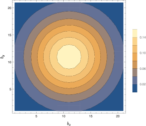
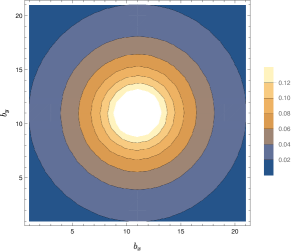
Figure 1: The digluon distribution $\tilde{F}_{gg}(x_{1}=10^{-4},x_{2}=10^{-2},b_{\perp},Q^{2}=m_{H}^{2})$. Left panel: calculation within the HO model. Right panel: calculation within the HP model. Partonic distance expressed in [GeV^-1].

In Fig. 1 we present the digluon dPDFs, evaluated within the HO (left panel) and HP (right panel) models at $Q^{2}=m_{H}^{2}$ in $\vec{b}_{\perp}$-space. Since we consider unpolarized partons in an unpolarized proton, circular symmetry in $\vec{b}_{\perp}$ is obtained, as apparent from the plot. Furthermore, the shape of the distributions are qualitatively similar to those shown in Ref. [12], where valence quark dPDFs have been evaluated within the same models but at the hadronic scale. By using these quantities, we have also evaluated the mean gluonic distance via Eqs. (8,14). The results, reported in Tab. 1, show that partonic correlations induce a dependence of the mean partonic distance upon the longitudinal momentum fractions carried by two partons. We recall that if correlations between $x_{i}$ and $k_{\perp}$ were absent, as in the non relativistic limit of dPDFs evaluated within the HO model (see Ref. [9]), the mean partonic distance would not depend on $x$’s and reads $\sqrt{\langle b^{2}\rangle}=0.283$ fm.

Kinematics	HO model	HP model
$x_{1},x_{2}$	$\sqrt{\langle b^{2}\rangle_{x_{1},x_{2}}}$ [fm]	$\sqrt{\langle b^{2}\rangle_{x_{1},x_{2}}}$ [fm]
$10^{-4},10^{-4}$	0.393	0.391
$10^{-4},10^{-2}$	0.382	0.408
$10^{-4},0.4~{}~{}$	0.393	0.405
$10^{-3},10^{-3}$	0.383	0.407
$10^{-2},10^{-2}$	0.365	0.404
$10^{-2},0.4~{}~{}~{}$	0.377	0.377

Table 1: Mean intergluon distance evaluated via dPDFs calculated at the scale $Q^{2}=m_{H}^{2}$ with the HO and HP models in different $x_{1},x_{2}$ configuration.

This discussion, however, is rather academic since the present accuracy of DPS measurements is far from being sensitive to this kind of effects. Nevertheless we have shown in Ref. [25] that physical information on the proton structure can still be directly obtained from $\sigma_{eff}$, a quantity which is often used in experimental analyses. In next sections we review the formalism that allows one to relate $\sigma_{eff}$ to $\langle b^{2}\rangle$, and generalize it to more complicated cases.

4 Transverse Proton structure from effective cross section

Double PDFs, the main non-perturbative ingredients appearing in the cross section formula in Eq. (4), are basically unknown, so that the direct application of the methods outlined in the previous Section can not be presently used. In this Section we discuss an alternative method that allows us to obtain information on the proton structure starting from experimental extracted quantities such as $\sigma_{eff}$. We proceed in the analysis with an increasing degree of complexity: in the first part of the Section, we find useful to summarize the strategy of the evaluation for the most simple case, i.e. a fully factorized ansatz of dPDFs [25]. In the second part, we generalize the results to include the so called splitting contribution to dPDFs which embodies correlations of perturbative origin. In the third part we generalize these results to unfactorized ansatz for dPDFs. In the last part of the Section all these results have been combined in a fully general relation between $\sigma_{eff}$ and $\langle b^{2}\rangle_{x_{1},x_{2}}$.

4.1 The factorized case

In Ref. [25] we have derived a relation between $\sigma_{eff}$ and the mean transverse partonic distance within the most simple assumptions on dPDFs, the fully factorized ansatz:

$$F_{ij}(x_{1},x_{2},k_{\perp})\sim q_{i}(x_{1})q_{j}(x_{2})f(k_{\perp})\,,$$ (15)

where $q_{i}(x)$ are ordinary single PDFs and $f(k_{\perp})$ is the effective form factor defined in Eq. (5). Usually, in such a simplified approach, $f(k_{\perp})$ does not depend on the parton flavors nor on fractional momenta [5, 30]. These assumptions allows to rewrite the DPS cross section as [7, 59]

$$d\sigma_{DPS}^{A+B}=\frac{m}{2}\dfrac{d\sigma_{SPS}^{A}\,d\sigma_{SPS}^{B}}{\sigma_{eff}}~{},$$ (16)

being $d\sigma_{SPS}^{A(B)}$ the single parton scattering cross sections with final state $A(B)$. In this scenario $\sigma_{eff}$ simply reads:

$$\sigma_{eff}^{-1}=\int{d^{2}k_{\perp}\over(2\pi)^{2}}f(k_{\perp})^{2}~{}{=\int{dk_{\perp}\over 2\pi}k_{\perp}f(k_{\perp})^{2}},$$ (17)

where the last expression follows from rotational invariance. Eq. (16) shows that, in such an approximations, $\sigma_{eff}$ enters the DPS cross section as an overall normalization factor. We remark that the EFF entering in the above is defined similarly to that in Eq. (5) but without the partonic flavor dependence, as often assumed in the experimental analyses in which $\sigma_{eff}$ is extracted. In Ref. [25], we have shown that, by using the formal definition of the EFF in Eq. (5) and appearing in Eq. (17), one can relate $\sigma_{eff}$ to the mean partonic distance of two partons active in a DPS process. We will briefly review this procedure in the following. As discussed in e.g. Refs. [58, 30, 25, 12], the EFF is the FT of the probability distribution of finding two parton at a given transverse distance, i.e. $\tilde{f}(b_{\perp})$, in a confined quantum mechanical system:

$$f(k_{\perp})=\int d^{2}b_{\perp}~{}e^{\vec{k}_{\perp}\cdot\vec{b}_{\perp}}\tilde{f}(b_{\perp}).$$ (18)

In terms of the latter, $\sigma_{eff}$ Eq. (17) is simply given by:

$$\sigma_{eff}^{-1}=\int d^{2}b_{\perp}~{}\tilde{f}(b_{\perp})^{2}~{},$$ (19)

see e.g. Refs. [30, 59, 29]. The latter expression relies on the probabilistic interpretation of $\tilde{f}(b_{\perp})$: this quantity represents the probability of finding a pair of partons at transverse distance $b_{\perp}$ [30, 59, 29]. This condition imposes the following normalization:

$$\int d^{2}b_{\perp}~{}\tilde{f}(b_{\perp})=1~{}.$$ (20)

This is a common assumption used in many phenomenological analyses of $\sigma_{eff}$, see e.g. Ref. [30]. The probabilistic interpretation of $\tilde{f}(b_{\perp})$ is transparent, for example, in the non relativistic limit. In fact, by considering Eq.(5), one gets:

$$\tilde{f}(b_{\perp}) =\int\frac{\displaystyle d^{2}k_{\perp}}{\displaystyle(2\pi)^{2}}~{}e^{-i\vec{k}_{\perp}\cdot\vec{b}_{\perp}}f(k_{\perp})$$ (21)

$$=\int\frac{\displaystyle d^{2}k_{\perp}}{\displaystyle(2\pi)^{2}}~{}e^{-i\vec{k}_{\perp}\cdot\vec{b}_{\perp}}\int d\vec{k}_{1}d\vec{k}_{2}~{}\Psi^{\dagger}(\vec{k}1+\vec{k}_{\perp},\vec{k}_{2})\Psi(\vec{k}_{1},\vec{k}_{2}+\vec{k}_{\perp})$$

$$\propto\int d\vec{b}_{1}d\vec{b}_{2}~{}|\tilde{\Psi}(\vec{b}_{1},\vec{b}_{2})|^{2}\delta^{(2)}(\vec{b}_{2\perp}-\vec{b}_{1\perp}-\vec{b}_{\perp})~{},$$

where here $\tilde{\Psi}(\vec{b}_{1},\vec{b}_{2})$ is the proton wave function in coordinate space and $b_{i}$ is the position of the parton $i$ in center mass frame. In terms of the EFF, two asymptotic conditions, related to the above features, can be obtained similarly to the standard form factors:

$$f(k_{\perp}=0)=1\;\;\mbox{and}~{}f(k_{\perp}\rightarrow\infty)=0~{}.$$ (22)

As discussed in Ref. [12], due to rotational invariance in the unpolarized case, Eq. (18) reduce to:

$$f(k_{\perp})=2\pi\int db_{\perp}~{}b_{\perp}J_{0}(b_{\perp}k_{\perp})\tilde{f}(b_{\perp})~{}.$$ (23)

The above can be expanded as follows [25]:

$$f(k_{\perp})=\sum_{n=0}^{\infty}{k_{\perp}^{2n}\langle b^{2n}_{\perp}\rangle}P_{n}^{J_{0}}\,,$$ (24)

where the $P_{n}^{J_{0}}$ are the expansion coefficients of the Bessel function and $\langle b^{2n}\rangle$ are weighted moments containing the dynamical information on the partonic proton structure. Let us remind that then mean partonic distance can be defined by means of the probability distribution in a standard way:

$$\langle b^{2}_{\perp}\rangle=\int d^{2}b_{\perp}~{}b_{\perp}^{2}\tilde{f}(b_{\perp})~{}.$$ (25)

In the following subsections we discuss the main steps to get a lower and upper bounds for $\langle b^{2}_{\perp}\rangle$ given a measured $\sigma_{eff}$ once the scenario Eq. (17) is assumed.

4.1.1 The minimum

Let us start with the minimum. By using the properties previously discussed (22) one can show that:

$$\int_{0}^{\infty}dk_{\perp}~{}f(k_{\perp})^{s-1}{d\over dk_{\perp}}f(k_{\perp})=-{1\over s}~{},$$ (26)

with $s>0$. In Ref. [25], in order to evaluate the minimum of the mean transverse distance, a useful relation between the integral Eq. (17) and $\langle b^{2}_{\perp}\rangle$ has been found. To this aim let us define the following function:

$$d_{2}(k_{\perp})=-2\frac{f^{\prime}(k_{\perp})}{k_{\perp}}=-4\sum_{n=1}k_{\perp}^{2n-2}\langle b^{2n}\rangle~{}P_{n}^{J_{0}}n~{}.$$ (27)

For simplicity we use the notation $\langle b^{2}_{\perp}\rangle\equiv\langle b^{2}\rangle$. One may notice that $\langle b^{2}\rangle=d_{2}(k_{\perp}=0)$, similarly to the case of the standard form factors and the charge radius of the proton. The above function is normalized as follows:

$$\int_{0}^{\infty}dk_{\perp}~{}k_{\perp}d_{2}(k_{\perp})=2~{}.$$ (28)

By using the identity Eq. (26) with $s=3$ one gets

$$-\frac{1}{3} =\int_{0}^{\infty}dk_{\perp}~{}f(k_{\perp})^{2}f^{\prime}(k_{\perp})=-\frac{1}{2}\int_{0}^{\infty}dk_{\perp}~{}k_{\perp}f(k_{\perp})^{2}d_{2}(k_{\perp})=$$ (29)

$$=2\int_{0}^{\infty}dk_{\perp}~{}f(k_{\perp})^{2}\sum_{n=1}k_{\perp}^{2n-1}\langle b^{2n}\rangle P_{n}n=$$

$$=\int_{0}^{\infty}dk_{\perp}~{}f(k_{\perp})^{2}\left[-\frac{\langle b^{2}\rangle k_{\perp}}{2}+2\sum_{n=2}k_{\perp}^{2n-1}\langle b^{2n}\rangle P_{n}n\right]=$$

$$=-\int_{0}^{\infty}dk_{\perp}~{}f(k_{\perp})^{2}\frac{\langle b^{2}\rangle k_{\perp}}{2}+2\sum_{n=2}\langle b^{2n}\rangle P_{n}n\int_{0}^{\infty}dk_{\perp}~{}k_{\perp}^{2n-1}f(k_{\perp})^{2}~{},$$

where the expansion in Eq. (27) has been used. The above expression can be rearranged to obtain:

$$\int_{0}^{\infty}dk_{\perp}~{}k_{\perp}f(k_{\perp})^{2}=\frac{2}{3\langle b^{2}\rangle}+4\sum_{n=2}P_{n}n\frac{\langle b^{2n}\rangle}{\langle b^{2}\rangle}\int_{0}^{\infty}dk_{\perp}~{}f(k_{\perp})^{2}k_{\perp}^{2n-1}~{}.$$ (30)

In the above equations we set $P_{n}=P_{n}^{J_{0}}$ for the sake of brevity. By using variance property, i.e. $\langle b^{n}\rangle\geq\langle b\rangle^{n}$, one can show that the second term on the right hand side of Eq. (30) is positive defined, thus leading to the condition:

$$\int_{0}^{\infty}dk_{\perp}~{}k_{\perp}f(k_{\perp})^{2}\geq\frac{2}{3\langle b^{2}\rangle}~{}.$$ (31)

The above condition, combined with the definition in eq. (17), allows one to find a minimum for $\langle b^{2}\rangle$, i.e.:

$$\langle b^{2}\rangle\geq\frac{\displaystyle\sigma_{eff}}{\displaystyle 2\pi}~{}.$$ (32)

4.1.2 The maximum

Let us now discuss the procedure, given a value of $\sigma_{eff}$, to obtain a maximum for $\langle b^{2}\rangle$ in the approximation of eq. (17). In this, more involved, case one should solve the following inequality

$$\dfrac{2\pi}{\sigma_{eff}}=\int_{0}^{\infty}dk_{\perp}~{}k_{\perp}f(k_{\perp})^{2}\leq\dfrac{1}{N\langle b^{2}\rangle}~{},$$ (33)

with $N$ a generic real number. The above expression is equivalent to the following:

$$\int_{0}^{\infty}dk_{\perp}~{}k_{\perp}f(k_{\perp})\Big{[}Nf(k_{\perp})\langle b^{2}\rangle-d_{2}(k_{\perp})\Big{]}\leq 0~{}.$$ (34)

The sufficient, but not necessary, condition to solve the above inequality is:

$$N\langle b^{2}\rangle f(k_{\perp})\leq d_{2}(k_{\perp})~{}.$$ (35)

By using the series expansion of $f(k_{\perp})$ and $d_{2}(k_{\perp})$, Eqs. (24-27) respectively, and by using the variance property, one gets:

$$N\sum_{n=0}P_{n}k_{\perp}^{2n}\langle b^{2n+2}\rangle\leq\sum_{n=0}\frac{P_{n}}{n+1}k_{\perp}^{2n}\langle b^{2n+2}\rangle~{}.$$ (36)

By shifting from $n$ to $n=\tilde{n}-1$, one then obtains:

$$N\sum_{\tilde{n}=1}P_{\tilde{n}-1}k_{\perp}^{2\tilde{n}-2}\langle b^{2\tilde{n}}\rangle\leq\sum_{\tilde{n}=1}\frac{P_{\tilde{n}-1}}{\tilde{n}}k_{\perp}^{2\tilde{n}-2}\langle b^{2\tilde{n}}\rangle~{}.$$ (37)

In principle one can solve the above inequality by comparing equal powers of $k_{\perp}$, i.e.: $P_{\tilde{n}-1}N\leq P_{\tilde{n}-1}/\tilde{n}$. Since the function $P_{n}$ changes sign with $n$, one finds:

$$\left\{\begin{array}[]{l}N\leq\dfrac{1}{\tilde{n}}~{}~{}\mbox{for $\tilde{n}$ odd}\\ \\ \\ N\geq\dfrac{1}{\tilde{n}}~{}~{}\mbox{for $\tilde{n}$ even}\end{array}\right.$$ (42)

Therefore $P_{\tilde{n}-1}$ is positive for $\tilde{n}$ odd and negative for $\tilde{n}$ even. Analytically one finds a chain of solutions:

$$\underbrace{\frac{1}{2}}_{\tilde{n}=2}\leq N\leq\underbrace{\frac{1}{1}}_{\tilde{n}=1};~{}~{}~{}\underbrace{\frac{1}{4}}_{\tilde{n}=4}\leq N\leq\underbrace{\frac{1}{3}}_{\tilde{n}=3};~{}~{}.....$$ (43)

One can generalize the above result in the following form:

$$\frac{1}{\tilde{n}}\leq N\leq\frac{1}{\tilde{n}-1}~{},~{}~{}~{}~{}\mbox{with}~{}~{}~{}~{}\tilde{n}~{}\mbox{even}~{},$$ (44)

or, in terms of the original $n$ ($\tilde{n}=n+1$):

$$\frac{1}{n+1}\leq N\leq\frac{1}{\ n}~{},~{}~{}~{}~{}\mbox{with}~{}~{}~{}~{}n~{}\mbox{odd}~{}.$$ (45)

As discussed in Ref. [25], in order to find a truncation on the above chain, some conditions on the behaviour of the EFF must be imposed even if the EFF, defined through Eq. (5), is essentially unknown. To this aim, we found that a comparison between the EFF and the standard one could guide toward a solution of the problem. In fact, similarly to standard case [66], at large $k_{\perp}$, i.e. in the pQCD domain, dynamical correlations between partons tend to decrease. In this case, it reasonable to expect that the EFF would be close to the product of standard form factors [61] whose asymptotic behaviours are $1/Q^{4}$ (Dirac) and $1/Q^{6}$ (Pauli). These conditions could be not true in all domain of $k_{\perp}$ but they are expected in the large $k_{\perp}$ limit, allowing to cut the chain in Eq. (43). On a more quantitative level, the condition required to solve the inequality (33) is that, at large $k_{\perp}$, the function $f(k_{\perp})$ should fall to zero at least as $k_{\perp}^{-2r}$ with $r>1$. As discussed in Ref. [25], this conjecture is supported by all model calculations of dPDF (even those not built up to calculate dPDFs). In particular let us mention that one of the most used dPDF ansatz makes use of EFF which is the product of the gluon form factor which satisfies the asymptotic condition mentioned above. Under the hypothesis that the EFF falls off at large $k_{\perp}$ as $k_{\perp}^{-2r}$ with $r>1$, then the $n=1$ contribution to the chain (43) is the dominant one, thus:

$$\dfrac{1}{2}\leq N\leq 1~{}.$$ (46)

In particular, since in Eq. (33) we are interested in $1/N$, we found that $1\leq 1/N\leq 2$. Collecting these results one finds:

$$\dfrac{2\pi}{\sigma_{eff}}=\int_{0}^{\infty}dk_{\perp}~{}k_{\perp}f(k_{\perp})^{2}\leq\dfrac{2}{\langle b^{2}\rangle}~{},$$ (47)

which is the desidered result. Combining all results, one gets:

$${\sigma_{eff}\over 3\pi}\leq\langle b^{2}\rangle\leq{\sigma_{eff}\over\pi}~{},$$ (48)

which is the main result of Ref. [25]. The above relation has been checked within all models of the EFF in the literature. Let us remark that in order to make contact with experimental extraction of $\sigma_{eff}$, this result has been obtained under the approximation of Eq.(17). Thanks to this feature, data on $\sigma_{eff}$ have been converted in the range of $\langle b^{2}\rangle$ [25]. In the following Sections we will describe how $\sigma_{eff}$ can be generalized to include partonic perturbative and non perturbative correlations, thus breaking the factorized ansatz in Eq. (17), and discuss how these correlations modify the relationship between $\langle b^{2}\rangle$ and $\sigma_{eff}$ in Eq.(48).

4.2 Generalization to 2v1 case

As discussed in Ref. [17, 28, 29, 30, 31, 32, 35, 60], the DPS cross section might receive a contribution from the so called 2v1 mechanism. In this case, one parton pair active in the processes is perturbatively produced from the splitting of a single parton, e.g. $g\rightarrow gg$, see the right panel of Fig. 2. Given the large gluon flux at LHC energies, such a contribution can be non-negligible [35] for double quarkonia and/or Higgs production [30] with respect to the standard 2v2 mechanism shown in the left panel of Fig. 2. This contribution breaks the simple ansatz in Eq. (17) and it is of pure perturbative origin. Its presence in dPDF evolution equation and in DPS cross sections has been carefully investigated [28, 31, 32, 56, 50, 60]. Within this mechanism, the separation of the parton pair is set by the hard scale in the splitting, $1/Q\ll b\ll 1/\Lambda$. Since one typically assumes that the non-perturbative $b$-profile has a width of order $1/\Lambda$, one can approximate $b=0$ in the 2v1 term[6, 30, 43, 60]. In this Section we consider the formalism developed in Refs. [30], where the $\sigma_{eff}$ definition is generalized to include the 2v1 contribution. As discussed in Ref. [30], one can decompose the total DPS cross section in terms of the two leading 2v2 and 2v1 contributions as follows

$$\sigma^{DPS}=\frac{\Omega^{2v2}}{\sigma_{eff,2v2}}+\frac{\Omega^{2v1}}{\sigma_{eff,2v1}}~{},$$ (49)

where here $\Omega^{2v2}$ and $\Omega^{2v1}$ represent the DPS cross sections calculated with longitudinal double PDFs for both mechanisms, and weighted by their corresponding $\sigma_{eff}$. In particular the $\Omega^{2v1}$ term is calculated with dPDFs whose initial condition is given by the splitting term alone at the initial scale [30]. As discussed in Ref. [30], in experimental analyses it is usually assumed that $\sigma^{DPS}=\Omega^{2v2}/\sigma_{eff}$. Within this approach, one can incorporate the 2v1 contribution in $\sigma^{DPS}$ by using the following generalization of $\sigma_{eff}$:

$$\frac{1}{\sigma_{eff}}=\frac{1}{\sigma_{eff,2v2}}+\frac{1}{\sigma_{eff,2v1}}\frac{\Omega^{2v1}}{\Omega^{2v2}}~{}.$$ (50)

Under the assumption that the longitudinal dependence of dPDFs factorizes from the transverse one, the effective cross sections for the two mechanisms read:

$$\frac{1}{\sigma_{eff,2v2}} =\int\frac{d^{2}k_{\perp}}{(2\pi)^{2}}f(k_{\perp})^{2}\,,$$ (51)

$$\frac{1}{\sigma_{eff,2v1}} =\int\frac{d^{2}k_{\perp}}{(2\pi)^{2}}f(k_{\perp})=\tilde{f}({\bf b_{\perp}}=0)\,,$$ (52)

where it is worth noticing that both the above expression depends on the same effective form factor, $f(k_{\perp})$, so that they are not independent quantities. The first equation is the standard one, see Eq. (17). The second one reflects the perturbative production of the couple of partons, occurring approximately at zero relative distance in transverse plane.

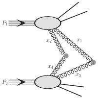
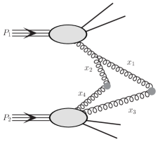
Figure 2: Diagrammatic representation of the two contributions to a DPS process: the so called 2v2 mechanisms is shown in the left panel and the 2v1 mechanism in the right panel. Small grey blobs represent the hard scattering processes.

In terms of the present notation, the main result of Ref. [25] reads:

$$\dfrac{1}{3\pi\langle b^{2}\rangle}\leq\dfrac{1}{\sigma_{eff,2v2}}\leq\dfrac{1}{\pi\langle b^{2}\rangle}~{},$$ (53)

where, by following Ref. [30], $\sigma_{eff,2v2}$ represents the usual definition of $\sigma_{eff}$ if only the 2v2 mechanism is considered, see Eq. (51). In the case where also the 2v1 mechanism is included in the analysis, in order to relate $\langle b^{2}\rangle$ to the experimentally extracted $\sigma_{eff}$ Eq. (50), we need first to find a relation between the mean partonic distance and $\sigma_{eff,2v1}$, defined in Eq. (52) and appearing in the full definition of $\sigma_{eff}$ in Eq. (50). To this aim, we can derive a new expression of the relevant integral with a procedure similar to the one already described in the first part of this section for the 2v2 mechanism:

$$\int_{0}^{\infty}dk_{\perp}~{}k_{\perp}f(k_{\perp})=\dfrac{1}{\langle b^{2}\rangle}+4\sum_{n=2}\dfrac{\langle b^{2n}\rangle P_{n}^{J_{0}}n}{\langle b^{2}\rangle}\int_{0}^{\infty}dk_{\perp}~{}k_{\perp}^{2n-1}f(k_{\perp})~{}.$$ (54)

Due to variance properties, the overall sign of the second term of the above equation is positive and consequently:

$$\dfrac{1}{\sigma_{eff,2v1}}\geq\dfrac{1}{2\pi\langle b^{2}\rangle}~{}.$$ (55)

Furthermore, similarly to the 2v2 case , in order to estimate a reasonable maximum, one needs solve the following inequality:

$$\int_{0}^{\infty}dk_{\perp}~{}k_{\perp}\left[\bar{N}f(k_{\perp})-\dfrac{d_{2}(k_{\perp})}{2}\right]\leq 0~{},$$ (56)

where $\bar{N}$ is an arbitrary unknown number. Under the additional assumption that the EFF falls to zero at large $k_{\perp}$ at least as fast as $k_{\perp}^{-2r}$ with $r\geq 1$, one finds the desired condition:

$$\dfrac{1}{\sigma_{eff,2v1}}\leq\dfrac{2}{\pi\langle b^{2}\rangle}~{}.$$ (57)

Linking Eq. (55) and Eq. (57), the following result is found:

$${\sigma_{eff,2v1}\over 2\pi}\leq\langle b^{2}\rangle\leq{2~{}\sigma_{eff,2v1}\over\pi}~{}.$$ (58)

Combining Eq.(53) and Eq.(58) in Eq. (50) one obtains the final inequality:

$$\dfrac{\sigma_{eff}}{3\pi}\left(1+\dfrac{3}{2}r_{v}\right)\leq\langle b^{2}\rangle\leq\dfrac{\sigma_{eff}}{\pi}\left(1+2r_{v}\right)~{},$$ (59)

where here we have defined the ratio $r_{v}=\Omega_{2v1}/\Omega_{2v2}$ , with $r_{v}\geq 0$. Let us remark that, in principle, the ratio $r_{v}$ could depend on the rapidities of particles produced in the final state and hence on parton fractional momenta in the initial state [30]. Such a dependence is not explored in the present analysis. The difference between the maximum and the minimum in Eq.(59) gives an estimate of the theoretical error on the transverse distance of the two active partons:

$$\Delta={\sigma_{eff}\over\pi}{2\over 3}\left(1+{9\over 4}r_{v}\right)~{}.$$ (60)

The main effect of the inclusion of the 2v1 mechanism is to shift the $\langle b^{2}\rangle$ range towards higher values and to increase its theoretical error with respect to the case where $r_{v}=0$. In particular, the comparison between the $r_{v}\neq 0$ and $r_{v}=0$ cases, makes sense only if $\sigma_{eff}$ is assumed to be equal in both scenarios. In principle, as observed in Refs. [28, 30], in order to observe $\sigma_{eff}\sim 15$ mb, one should expect $\sigma_{eff,2v2}\sim 30$ mb. In general, if $r_{v}\neq$1, from Eq. (50) one gets $\sigma_{eff}\leq\sigma_{eff,2v2}$.

We find interesting to check the validity of Eq. (59) by using two phenomenological models for EFF, such as those described in Refs. [28, 30, 61]. The first one is Gaussian EFF of the type:

$$f(k_{\perp})=e^{-k_{\perp}^{2}a}~{}.$$ (61)

In this case the mean partonic distance can be obtained in term of the width parameter $a$ as:

$$\langle b^{2}\rangle=-2\frac{d}{k_{\perp}dk_{\perp}}f(k_{\perp})\Bigg{|}_{k_{\perp}=0}=4a~{},$$ (62)

so that, according to Eqs. (51,52),

$$\sigma_{eff,2v2}=2\langle b^{2}\rangle\pi~{},\;\;\;\sigma_{eff,2v1}=\langle b^{2}\rangle\pi~{}.$$ (63)

By using the above expressions in Eq. (50), one gets the following result:

$$\langle b^{2}\rangle=\frac{\sigma_{eff}}{\pi}\left(\frac{1}{2}+r_{v}\right)~{},$$ (64)

which is included in the range Eq. (59). As a second example we consider an EFF which is the square of the gluon form factor [61], i.e.:

$$f(k_{\perp})=\left(\frac{k_{\perp}^{2}}{m_{g}^{2}}+1\right)^{-4}~{},$$ (65)

with the parameter $m_{g}$ has been fixed by fitting HERA data, i.e. $m_{g}^{2}\sim 1.1$ GeV² [61]. In this case one obtains:

$$\langle b^{2}\rangle=-2\frac{d}{k_{\perp}dk_{\perp}}f(k_{\perp})\Bigg{|}_{k_{\perp}=0}={16\over m_{g}^{2}}~{},$$ (66)

and, according to Eqs. (51,52),

$$\sigma_{eff,2v2}={7\over 4}\langle b^{2}\rangle\pi~{},~{}\sigma_{eff,2v1}={3\over 4}\langle b^{2}\rangle\pi~{}.$$ (67)

By using the above expressions in Eq. (50), one gets the following result:

$$\langle b^{2}\rangle=\frac{\sigma_{eff}}{\pi}\left(\frac{4}{7}+\frac{4}{3}r_{v}\right)~{},$$ (68)

which again lies in the range indicated in Eq. (59).

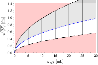
Figure 3: The averaged partonic interdistance as a function of $\sigma_{eff}$. Dashed lines represent the minimum of Eq. (69). Dot-dashed lines stand for the maximum of Eq. (69). Dotted lines are for the maximum of Eq. (48). Vertical lines represent the full range of allowed partonic distances between two partons if the 2v2 and the 2v1 mechanism effects on the total $\sigma_{eff}$ are not disentangled. The shadow between lines represents the additional theoretical error w.r.t. the case where only the 2v2 mechanism is considered, i.e. Eq. (48). The areas outside lines represent the exclusion region of the allowed transverse distance between two partons active in a DPS process. The red line stands for twice the transverse proton radius.

Such a generalization of the inequality in Eq. (48) is however process dependent, in fact, as discussed in Refs. [28, 30], $r_{v}$ is related to the kinematic conditions and to the type of the considered DPS process. Without a precise knowledge on $r_{v}$, a determination of the range of the allowed mean partonic transverse distance is therefore prevented. Nonetheless, we note that $r_{v}\geq 0$ since it is a ratio of cross sections which is positive definite. Furthermore one expects that $r_{v}\leq 1$, at least for processes involving small parton fractional momenta, as those typically considered in the present analysis. Additionally, in this regime, one expects the 2v1 mechanism to be subdominant in the pQCD evolution of dPDFs w.r.t. the 2v2 one, being the former proportional to the gluon density and the latter proportional to its square. Thanks to these features, for $r_{v}=0$ one finds the minimum in Eq. (59) while for $r_{v}=1$ one finds its maximum:

$$\dfrac{\sigma_{eff}}{3\pi}\leq\langle b^{2}\rangle\leq\dfrac{3\sigma_{eff}}{\pi}~{}.$$ (69)

This result allows one to obtain information on the interpartonic distance of two active partons in a DPS process without knowing details on the relative size of the two mechanisms, 2v1 and 2v2, i.e. the exact knowledge of $r_{v}$. This, of course, comes at the expense of an increased theoretical error. In order to quantify such an effect, we have plotted in Fig. 3 the two extremes of Eq. (69) with dashed and dot-dashed lines respectively, together with the maximum of Eq. (59) evaluated with $r_{v}=0$ (dotted lines), as function of different values of $\sigma_{eff}$. The white area between the curves represents the theoretical error associated to the 2v2 mechanism alone. The shaded area represents the additional uncertainty induced by the particular choice on $r_{v}$ leading to Eq. (69). In addition, in Table 2, we report the interpartonic distances, calculated according to Eq. (59), for $\sigma_{eff}$ values extracted from a selection of experimental analyses. It should be noted that, in all cases, $\sqrt{\langle b^{2}\rangle}<2R_{\perp}=1.42$ fm, where $R_{\perp}\sim 0.71$ fm is the transverse electro-magnetic proton radius.

Ref.	Process	$\sigma_{eff}$ [mb]	$\sqrt{{\sigma_{eff}\over 3\pi}}$ [fm]	$\sqrt{{3\sigma_{eff}\over\pi}}$[fm]
[72]	D0$~{}(J/\Psi+\Upsilon),~{}\sqrt{s}=1.96$ TeV	$\sim 2.2$	0.15	0.46
[73]	$(J/\Psi+Z),~{}\sqrt{s}=8$ TeV	$\sim 4.7$	0.22	0.67
[47]	D0$~{}(J/\Psi+J/\Psi),~{}\sqrt{s}=1.96$ TeV	$\sim 4.8$	0.23	0.68
[74]	$(W+J/\Psi),~{}\sqrt{s}=7$ TeV	$\sim 6.1$	0.25	0.76
[23]	ATLAS $(J/\Psi+J/\Psi),~{}\sqrt{s}=8$ TeV	$\sim 6.3$	0.26	0.78
[24]	$(J/\Psi+J/\Psi),~{}\sqrt{s}=7$ TeV	$\sim 8.2$	0.29	0.88
[20]	LHCb $(J/\Psi+J/\Psi),~{}\sqrt{s}=13$ TeV	$\sim 8.8$	0.31	0.92
[19]	ATLAS (4-jets) $\sqrt{s}=7$ TeV	$\sim 14.9$	0.40	1.19
[75]	LHCb $(\Upsilon+c\bar{c}),~{}\sqrt{s}=7-8$ TeV	$\sim 18.0$	0.44	1.31
[21]	CMS (W+2-jets) $\sqrt{s}=7$ TeV	$\sim 20.7$	0.47	1.41

Table 2: Ranges of mean transverse distance evaluated by means of Eq. (69) sorted by increasing values of $\sigma_{eff}$ as extracted from the quoted experimental analyses.

We close this Section by observing that Eq. (59) can be inverted to give:

$${\pi\langle b^{2}\rangle\over(1+2r_{v})}\leq\sigma_{eff}\leq{\pi\langle b^{2}\rangle 3\over\left(1+{3\over 2}r_{v}\right)}~{}.$$ (70)

In such a form, given the value of $\langle b^{2}\rangle$ associated to a particular $f(k_{\perp})$, the inequality in Eq. (70) predicts the expected range in $\sigma_{eff}$ associated to that specific model. Most importantly, Eq.(70) shows that, given an EFF, characterized by $\langle b^{2}\rangle$, the $\sigma_{eff}$ value does depend on the relative size of the 2v1 contribution. In particular, if $r_{v}$ is significantly larger than zero, the corresponding $\sigma_{eff}$ will be lower than the one obtained if the 2v2 mechanism alone were considered ($r_{v}=0$).

4.3 Generalization to the unfactorized ansatz

As shown in several constituent quark model calculations of dPDFs, double parton correlations may survive at high momentum transfer, which are relevant for experimentally measurable processes [8, 9, 11, 12, 46, 57]. In this Section we investigate how Eq. (48) is generalized to the case in which the factorized ansatz is not assumed thus allowing the presence of longitudinal and mixed longitudinal-transverse partonic correlations. We consider an unapproximated scenario in which $\sigma_{eff}$ depends on the longitudinal momentum fractions of the active partons, as suggested in Refs. [58, 62]. Within this improved framework, the relationship between $\sigma_{eff}$ and the mean partonic distance will be sensitive to $x_{1}-x_{2}$ correlations. For this purpose we consider the simplest generalization of the results presented in Section 3, namely we consider non-factorizable dPDFs, in the zero rapidity case, i.e. $x_{i}=x_{i}^{\prime}$. For processes whose production is dominated by gluons, as those discussed in this paper, the expression for $\sigma_{eff}$ can be simplified to [58]:

$$\sigma_{eff}(x_{1},x_{2})=2\pi\frac{\displaystyle\big{[}F(x_{1})F(x_{2})\big{]}^{2}}{\displaystyle\int dk_{\perp}~{}k_{\perp}F(x_{1},x_{2},k_{\perp})^{2}}~{},$$ (71)

where $F(x)$ and $F(x_{1},x_{2})$ represent single and double gluon PDFs, respectively. We assume that the $k_{\perp}$ dependence of dPDFs has the same behaviour and asymptotics as the ones discussed for the EFF in Sec. 3. This feature is inspired by the GPDs behavior, whose dependence on the transverse momentum basically follows the one of the related form factor. In the present case the inequality is obtained following the same steps outlined in Section 4, but retaining the full $(x_{1},x_{2})$ dependence via dPDFs. To this aim we expand the form factor as:

$$F(x_{1},x_{2},k_{\perp}) =2\pi\int db_{\perp}~{}b_{\perp}J_{0}(k_{\perp}b_{\perp})\tilde{F}(x_{1},x_{2},b_{\perp})=$$ (72)

$$=\sum_{n=0}^{\infty}k_{\perp}^{2n}~{}P_{n}^{J_{0}}\int d^{2}b_{\perp}~{}b_{\perp}^{2n}\tilde{F}(x_{1},x_{2},b_{\perp})~{}.$$

By using the definition in Eq. (8) one can derive the following expression:

$$\dfrac{F(x_{1},x_{2},k_{\perp})}{F(x_{1},x_{2},0)}=\sum_{n=0}^{\infty}{k_{\perp}^{2n}\langle b_{\perp}^{2n}\rangle_{x_{1},x_{2}}}P_{n}^{J_{0}}\,.$$ (73)

4.3.1 The minimum

The strategy to get a relation between $\sigma_{eff}$ and $\langle b_{\perp}^{2}\rangle_{x_{1},x_{2}}$ is then very similar to the one we discussed in Sect. 4.1.1. Eqs. (26, 27) can be generalized to

$$\int_{0}^{\infty}dk_{\perp}~{}F(x_{1},x_{2},k_{\perp})^{s-1}{d\over dk_{\perp}}F(x_{1},x_{2},k_{\perp})=-{F(x_{1},x_{2},0)^{s}\over s}~{},$$ (74)

and the derivative function to:

$$d_{2}^{x_{1},x_{2}}(k_{\perp})=-\frac{\displaystyle 2}{\displaystyle F(x_{1},x_{2},0)}\frac{\displaystyle F^{\prime}(x_{1},x_{2},k_{\perp})}{\displaystyle k_{\perp}}=-4\sum_{n=1}^{\infty}k_{\perp}^{2n-2}\langle b_{\perp}^{2n}\rangle_{x_{1},x_{2}}P_{n}n~{}.$$ (75)

In this case, $\langle b_{\perp}^{2}\rangle_{x_{1},x_{2}}=d_{2}^{x_{1},x_{2}}(k_{\perp}=0)$. Within these settings we generalize Eq. (30) to obtain the first relation between $\sigma_{eff}(x_{1},x_{2})$ and $\langle b_{\perp}^{2}\rangle_{x_{1},x_{2}}$. As in Sect. 4.1.1, we start with Eq. (74) for $s=3$:

$$-\frac{\displaystyle F(x_{1},x_{2},0)^{3}}{\displaystyle 3} =\int_{0}^{\infty}dk_{\perp}~{}F(x_{1},x_{2},k_{\perp})^{2}F^{\prime}(x_{1},x_{2},k_{\perp})$$ (76)

$$=-\frac{\displaystyle F(x_{1},x_{2},0)}{\displaystyle 2}\int_{0}^{\infty}dk_{\perp}~{}k_{\perp}F(x_{1},x_{2},k_{\perp})^{2}d_{2}^{x_{1},x_{2}}(k_{\perp})$$

$$=F(x_{1},x_{2},0)2\int_{0}^{\infty}dk_{\perp}~{}F(x_{1},x_{2},k_{\perp})^{2}\sum_{n=1}^{\infty}k_{\perp}^{2n-1}\langle b_{\perp}^{2n}\rangle_{x_{1},x_{2}}P_{n}n$$

$$=F(x_{1},x_{2},0)\int_{0}^{\infty}dk_{\perp}~{}F(x_{1},x_{2},k_{\perp})^{2}\left[-\frac{\displaystyle\langle b_{\perp}^{2}\rangle_{x_{1},x_{2}}k_{\perp}}{\displaystyle 2}+2\sum_{n=2}^{\infty}k_{\perp}^{2n-1}\langle b_{\perp}^{2n}\rangle_{x_{1},x_{2}}P_{n}n\right]$$

$$=-F(x_{1},x_{2},0)\int_{0}^{\infty}dk_{\perp}~{}k_{\perp}F(x_{1},x_{2},k_{\perp})^{2}\frac{\displaystyle\langle b_{\perp}^{2}\rangle_{x_{1},x_{2}}}{\displaystyle 2}$$

$$+2F(x_{1},x_{2},0)\sum_{n=2}^{\infty}\langle b_{\perp}^{2n}\rangle_{x_{1},x_{2}}P_{n}n\int_{0}^{\infty}dk_{\perp}~{}k_{\perp}^{2n-1}F(x_{1},x_{2},k_{\perp})^{2}~{}.$$

Finally one gets:

$$\int_{0}^{\infty}dk_{\perp}~{}k_{\perp}F(x_{1},x_{2},k_{\perp})^{2} =\dfrac{2}{3}\frac{\displaystyle F(x_{1},x_{2},0)^{2}}{\displaystyle\langle b_{\perp}^{2}\rangle_{x_{1},x_{2}}}$$ (77)

$$+4\sum_{n=2}^{\infty}\frac{\displaystyle\langle b_{\perp}^{2n}\rangle_{x_{1},x_{2}}}{\displaystyle\langle b_{\perp}^{2}\rangle_{x_{1},x_{2}}}\int_{0}^{\infty}dk_{\perp}~{}F(x_{1},x_{2},k_{\perp})^{2}k_{\perp}^{2n-1}~{}.$$

By noticing that the second term is positive definite, one obtains the following inequality:

$$\int_{0}^{\infty}dk_{\perp}~{}k_{\perp}F(x_{1},x_{2},k_{\perp})^{2}\geq\dfrac{2}{3}\frac{\displaystyle F(x_{1},x_{2},0)^{2}}{\displaystyle\langle b_{\perp}^{2}\rangle_{x_{1},x_{2}}}~{}.$$ (78)

In terms of $\sigma_{eff}(x_{1},x_{2})$ defined in Eq. (71) the result is recast into:

$$\frac{\displaystyle\langle b_{\perp}^{2}\rangle_{x_{1},x_{2}}}{\displaystyle r_{gg}(x_{1},x_{2})^{2}}\geq\frac{\displaystyle\sigma_{eff}(x_{1},x_{2})}{\displaystyle 3\pi}~{},$$ (79)

where we defined:

$$r_{gg}(x_{1},x_{2})={F(x_{1},x_{2},k_{\perp}=0)\over F(x_{1})F(x_{2})}~{}.$$ (80)

4.3.2 The maximum

In this last part we derive the maximum of the mean transverse distance for a unfactorized dPDFs ansatz. Also in this case we consider a general realistic condition, i.e. the $k_{\perp}$ dependence of dPDFs is dominated by that of the EFF. In this scenario, the only difference between this case and the previous one, see Sec. 4.1, is that for fixed values of $x_{1}$, $x_{2}$ and the energy scale, the dPDF at $k_{\perp}=0$ can be different from 1. In this case it is necessary to find a value of $N$ such that:

$$\frac{\displaystyle 2\pi}{\displaystyle\sigma_{eff}(x_{1},x_{2})}=\frac{\displaystyle\int_{0}^{\infty}dk_{\perp}~{}k_{\perp}F(x_{1},x_{2},k_{\perp})^{2}}{\displaystyle\Big{[}F(x_{1})F(x_{2})\Big{]}^{2}}\leq\frac{\displaystyle 1}{\displaystyle N\langle b_{\perp}^{2}\rangle_{x_{1},x_{2}}}~{}.$$ (81)

The above expression can be rearranged as follows:

$$\int_{0}^{\infty}dk_{\perp}~{}k_{\perp}F(x_{1},x_{2},k_{\perp})\left[F(x_{1},x_{2},k_{\perp})N\frac{\displaystyle r_{gg}(x_{1},x_{2})^{2}}{\displaystyle F(x_{1},x_{2},0)^{2}}-1\right]\leq 0~{}.$$ (82)

In order to find a sufficient condition to solve the above inequality, we make use of the following identity:

$$\int_{0}^{\infty}dk_{\perp}~{}k_{\perp}F(x_{1},x_{2},k_{\perp})d_{2}^{x_{1},x_{2}}(k_{\perp})=F(x_{1},x_{2},0)~{}.$$ (83)

By using the above expression, Eq. (82) becomes:

$$\int_{0}^{\infty}dk_{\perp}~{}k_{\perp}\frac{\displaystyle F(x_{1},x_{2},k_{\perp})}{\displaystyle F(x_{1},x_{2},0)}\left[\frac{\displaystyle F(x_{1},x_{2},k_{\perp})}{\displaystyle F(x_{1},x_{2},0)}Nr_{gg}(x_{1},x_{2})^{2}\langle b_{\perp}^{2}\rangle_{x_{1},x_{2}}-d_{2}^{x_{1},x_{2}}(k_{\perp})\right]\leq 0~{},$$ (84)

and a sufficient condition to solve the inequality reads:

$$\frac{\displaystyle F(x_{1},x_{2},k_{\perp})}{\displaystyle F(x_{1},x_{2},0)}Nr_{gg}(x_{1},x_{2})^{2}\langle b_{\perp}^{2}\rangle_{x_{1},x_{2}}\leq d_{2}^{x_{1},x_{2}}(k_{\perp})~{}.$$ (85)

By using Eqs. (73-74) the latter can be rewritten as:

$$N(x_{1},x_{2})\sum_{\tilde{n}=1}P_{\tilde{n}-1}k_{\perp}^{2\tilde{n}-2}\langle b_{\perp}^{2\tilde{n}}\rangle_{x_{1},x_{2}}\leq\sum_{\tilde{n}=1}\frac{\displaystyle P_{\tilde{n}-1}}{\displaystyle\tilde{n}}k_{\perp}^{2\tilde{n}-2}\langle b_{\perp}^{2\tilde{n}}\rangle_{x_{1},x_{2}}~{},$$ (86)

where we define $N(x_{1},x_{2})\equiv Nr_{gg}(x_{1},x_{2})^{2}$. The same chain of solutions shown in Eqs. (42-45) is obtained, the main difference being now that these solutions correspond to $N(x_{1},x_{2})$. Therefore one gets:

$$1\leq\dfrac{1}{N(x_{1},x_{2})}\leq 2~{},$$ (87)

which corresponds to:

$$r_{gg}(x_{1},x_{2})^{2}\leq\dfrac{1}{N}\leq 2~{}r_{gg}(x_{1},x_{2})^{2}~{}.$$ (88)

By using this relation in Eq. (81) one finds:

$$\frac{\displaystyle\langle b_{\perp}^{2}\rangle_{x_{1},x_{2}}}{\displaystyle r_{gg}(x_{1},x_{2})^{2}}\leq\frac{\displaystyle\sigma_{eff}}{\displaystyle\pi}$$ (89)

Combining Eq. (79) and Eq. (89) one finally obtains:

$${\sigma_{eff}(x_{1},x_{2})\over 3\pi}\leq\dfrac{\langle b^{2}\rangle_{x_{1},x_{2}}}{r_{gg}(x_{1},x_{2})^{2}}\leq{\sigma_{eff}(x_{1},x_{2})\over\pi}~{},$$ (90)

which, with respect to Eq. (48), additionally depends on the ratio $r_{gg}$. Such a ratio encodes longitudinal correlations in the proton structure, and therefore so does $\langle b^{2}\rangle_{x_{1},x_{2}}$.

Kinematics	HO model			HP model
	${\sigma_{eff}(x_{1},x_{2})\over 3\pi}$	${\langle b^{2}\rangle_{x_{1},x_{2}}\over r_{gg}^{2}(x_{1},x_{2})}$	${\sigma_{eff}(x_{1},x_{2})\over\pi}$	${\sigma_{eff}(x_{1},x_{2})\over 3\pi}$	${\langle b^{2}\rangle_{x_{1},x_{2}}\over r_{gg}^{2}(x_{1},x_{2})}$	${\sigma_{eff}(x_{1},x_{2})\over\pi}$
$x_{1}=10^{-4},x_{2}=10^{-4}$	0.263	0.429	0.790	0.235	0.425	0.704
$x_{1}=10^{-2},x_{2}=10^{-4}$	0.256	0.405	0.767	0.227	0.462	0.680
$x_{1}=10^{-2},x_{2}=10^{-2}$	0.268	0.370	0.805	0.226	0.453	0.678

Table 3: Numerical test of the validity of Eq. (90) by using the HO and HP models. Double gluon distributions have been evolved at $Q^{2}=m_{H}^{2}$. The various entries in the table are expressed in [$\mbox{fm}^{2}$].

In order to test the inequality, we have evaluated the terms appearing in Eq. (90), i.e. $\sigma_{eff}(x_{1},x_{2})$, $r_{gg}(x_{1},x_{2})$ and $\langle b^{2}\rangle_{x_{1},x_{2}}$, by using quark model calculations of dPDFs and PDFs, see Fig. 4 for $r_{gg}(x_{1},x_{2})$. Since we are interested in kinematic regions close to those experimentally accessed, we have calculated the above quantities by using the digluon dPDF obtained through pQCD evolution at high momentum scales, $Q^{2}=m_{H}^{2}$, and test Eq. (90) in three couples of fractional momenta, $x_{1}=x_{2}=10^{-4}$, $x_{1}=10^{-4},x_{2}=10^{-2}$ and $x_{1}=x_{2}=10^{-2}$. In addition, in order to assess the hadronic model dependence of the results, Eq. (90) has been calculated with digluon distribution obtained within two different CQMs. The results are reported Table 3 and, as one may notice, the inequality Eq. (90) is verified in all kinematic conditions. One should also notice that, at variance with the case where the factorization ansatz in Eq. (15) is assumed, in this new scenario the effects of correlations in dPDFs, embodied in the $r_{gg}(x_{1},x_{2})$ factor, play a crucial role in verifying the identity. This generalized inequality effectively allows one to estimate the impact of double parton correlations on the range of allowed parton transverse distances.

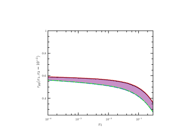
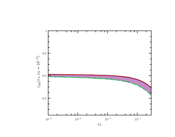
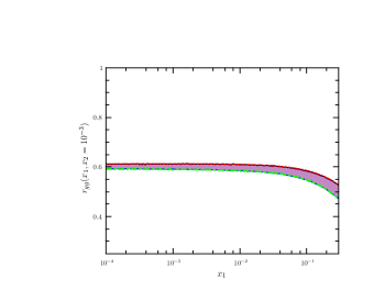
Figure 4: The ratio $r_{gg}(x_{1},x_{2})$, Eq. (80), evaluated at $x_{2}=10^{-1}$ (upper-left panel), $x_{2}=10^{-2}$ (upper-right panel), $x_{2}=10^{-3}$ (lower-left panel) and $x_{2}=10^{-4}$ (lower-right panel). The HO model predictions are indicated by full line ($Q^{2}=4m_{c}^{2}$) and dashed line ($Q^{2}=m_{H}^{2}$). The HP model predictions are indicated by dotted line ($Q^{2}=4m_{c}^{2}$) and dot-dashed line ($Q^{2}=m_{H}^{2}$). The band stands for the difference between the calculations performed in the two scales.

4.4 The full relation

In this final part we collect all previous results to obtain a full relation between $\sigma_{eff}$ and $\langle b_{\perp}^{2}\rangle_{x_{1},x_{2}}$ in the zero rapidity region including also the splitting contribution. In this case the full demonstration consists in a combination of the previous ones. From Sec. 4.1, we discussed the following system of relations if the splitting contribution is included:

$$\left\{\begin{array}[]{l}\dfrac{1}{\sigma_{eff}}=\dfrac{1}{\sigma_{eff,2v2}}+\dfrac{r_{v}}{\sigma_{eff,2v1}}\\ \\ \dfrac{\sigma_{eff,2v2}}{3\pi}\leq\langle b^{2}\rangle\leq\dfrac{\sigma_{eff,2v2}}{\pi}\\ \\ \dfrac{\sigma_{eff,2v1}}{2\pi}\leq\langle b^{2}\rangle\leq\dfrac{2\sigma_{eff,2v1}}{\pi}\end{array}\right.$$ (96)

As shown in Sec. 4.2, on the other hand side, if the $x_{1}-x_{2}$ and $k_{\perp}$ correlations are not neglected:

$$\dfrac{\sigma_{eff,2v2}(x_{1},x_{2})r_{gg}^{2v2}(x_{1},x_{2})^{2}}{3\pi}\leq\langle b^{2}\rangle_{x_{1},x_{2}}\leq\dfrac{\sigma_{eff,2v2}(x_{1},x_{2})r_{gg}^{2v2}(x_{1},x_{2})^{2}}{\pi}$$ (97)

where by definition $r_{gg}^{2v2}(x_{1},x_{2})=r_{gg}(x_{1},x_{2})=F(x_{1},x_{2},0;Q^{2})/[F(x_{1};Q^{2})F(x_{2};Q^{2})]$. Let us remark here that within this notation, $F(x_{1},x_{2},0;Q^{2})$ is the radiative digluon PDF as obtained from homogeneous evolution. In order to include correlations between $x_{1}-x_{2}$ and $k_{\perp}$ also in the case where the splitting contribution in the pQCD evolution is included, one may introduce a new ratio:

$$r_{gg}^{2v1}(x_{1},x_{2})=\dfrac{F^{splitting}_{gg}(x_{1},x_{2},0;Q^{2})}{F(x_{1};Q^{2})F(x_{2};Q^{2})}~{},$$ (98)

where $F^{splitting}_{gg}(x_{1},x_{2},0;Q^{2})$ is the pure splitting contribution to digluon dPDF where the non dPDFs are evolved with inhomogeneous evolution equations with the non peturbative digluon distribution set to zero at the intial scale. By performing the same steps previously discussed, one obtains

$$\dfrac{\sigma_{eff,2v1}(x_{1},x_{2})r_{gg}^{2v1}(x_{1},x_{2})^{2}}{2\pi}\leq\langle b^{2}\rangle_{x_{1},x_{2}}\leq\dfrac{2\sigma_{eff,2v1}(x_{1},x_{2})r_{gg}^{2v1}(x_{1},x_{2})^{2}}{\pi}$$ (99)

Combining all terms one gets:

$$\dfrac{\sigma_{eff}(x_{1},x_{2})}{3\pi}\left(r^{2v2}_{gg}(x_{1},x_{2})^{2}+\dfrac{3}{2}r^{2v1}_{gg}(x_{1},x_{2})^{2}r_{v}\right)\leq\langle b^{2}\rangle_{x_{1},x_{2}}\leq\dfrac{\sigma_{eff}(x_{1},x_{2})}{\pi}\Big{(}r^{2v2}_{gg}(x_{1},x_{2})^{2}+2r^{2v1}_{gg}(x_{1},x_{2})^{2}r_{v}\Big{)}~{}.$$ (100)

This last expression represents the most general inequality between the mean transverse partonic distance and $\sigma_{eff}(x_{1},x_{2})$. In order to avoid to model $r_{v}$, we may consider the maximum range by setting $r_{v}=0$ and $r_{v}=1$ in the minimum and maximum bounds respectively:

$$\dfrac{\sigma_{eff}(x_{1},x_{2})}{3\pi}\Big{[}r_{gg}^{2v2}(x_{1},x_{2})^{2}\Big{]}\leq\langle b^{2}\rangle_{x_{1},x_{2}}\leq\dfrac{\sigma_{eff}(x_{1},x_{2})}{\pi}\Big{[}r_{gg}^{2v2}(x_{1},x_{2})^{2}+2r_{gg}^{2v1}(x_{1},x_{2})^{2}\Big{]}~{}.$$ (101)

In Ref. [30], authors introduced a ratio between the splitting contribution term to dPDFs versus the dPDF evolved only with the homogeneous one:

$$r_{ga}(x_{1},x_{2})=\dfrac{F_{gg}^{splitting}(x_{1},x_{2},0;Q^{2})}{F_{gg}(x_{1},x_{2},0;Q^{2})}\geq 0~{}.$$ (102)

In their analysis, by considering different models and kinematic conditions, authors of Ref. [30] estimated that $r_{ga}(x_{1},x_{2})\leq 0.2$. One should notice that this quantity appear in Eqs. (100,101) by rewriting $r_{gg}^{2v1}(x_{1},x_{2})$ as follows:

$$r^{2v1}_{gg}(x_{1},x_{2}) =\dfrac{F_{gg}^{splitting}(x_{1},x_{2},0;Q^{2})}{F_{g}(x_{1};Q^{2})F_{g}(x_{2};Q^{2})}$$ (103)

$$=\dfrac{F_{gg}^{splitting}(x_{1},x_{2},0;Q^{2})}{F_{gg}(x_{1},x_{2},0;Q^{2})}\dfrac{F_{gg}(x_{1},x_{2},0;Q^{2})}{F_{g}(x_{1};Q^{2})F_{g}(x_{2};Q^{2})}$$

$$=r_{ga}(x_{1},x_{2})\cdot r^{2v2}_{gg}(x_{1},x_{2})~{}.$$

With this notation Eq. (101) becomes:

$$\dfrac{\sigma_{eff}(x_{1},x_{2})}{3\pi}\Big{[}r_{gg}^{2v2}(x_{1},x_{2})^{2}\Big{]}\leq\langle b^{2}\rangle_{x_{1},x_{2}}\leq\dfrac{\sigma_{eff}(x_{1},x_{2})}{\pi}r_{gg}^{2v2}(x_{1},x_{2})^{2}\Big{[}1+2~{}r_{ga}(x_{1},x_{2})^{2}\Big{]}~{}.$$ (104)

To date there are no published data on $\sigma_{eff}$ with an explicit evaluation of its dependence on $x_{1}$ and $x_{2}$. Therefore we can give an estimate of Eq. (104) with a costant $\sigma_{eff}$.

Ref.	Process	$\sigma_{eff}$ [mb]	$\sqrt{{\sigma_{eff}\over 3\pi}}0.6$ [fm]	$\sqrt{{0.4\sigma_{eff}\over\pi}}$[fm]
[72]	D0$~{}(J/\Psi+\Upsilon),~{}\sqrt{s}=1.96$ TeV	$\sim 2.2$	0.09	0.17
[47]	D0$~{}(J/\Psi+J/\Psi),~{}\sqrt{s}=1.96$ TeV	$\sim 4.8$	0.13	0.25
[23]	ATLAS $(J/\Psi+J/\Psi),~{}\sqrt{s}=8$ TeV	$\sim 6.3$	0.16	0.28
[24]	$(J/\Psi+J/\Psi),~{}\sqrt{s}=7$ TeV	$\sim 8.2$	0.18	0.32
[20]	LHCb $(J/\Psi+J/\Psi),~{}\sqrt{s}=13$ TeV	$\sim 8.8$	0.18	0.33
[75]	LHCb $(\Upsilon+c\bar{c}),~{}\sqrt{s}=7-8$ TeV	$\sim 18.0$	0.26	0.48

Table 4: Ranges of mean transverse distance evaluated from Eq. (104) setting $r_{ga}\sim 0.2$, $r_{gg}\sim 0.6$ and by pretending that the experimental $\sigma_{eff}$ is extracted by the non factorized dPDF.

In Tab. 4 we report numerical estimates of the allowed range of $\langle b_{\perp}\rangle_{x_{1},x_{2}}$, obtained by using Eq. (104) in the worst scenario, i.e. $r_{ga}\sim 0.2$ and $r_{gg}(x_{1},x_{2})\sim 0.6$. We note that in this last inequality the theoretical errors are reduced and the range of mean distance is shifted towards smaller values with respect to the ranges reported in Tab. 2 for the simple factorized case studied in Section 3. We also remark that the physical information accessible relies upon the approximations with which $\sigma_{eff}$ is extracted.

5 Relativistic effects in dPDFs

In this Section we consider relativistic effects on dPDFs, already addressed in Ref. [12], and study their relevance when propagated at high momentum transfer in typical LHC kinematics, with a special emphasis on the digluon distribution. Relativistic effects, in fact, induce model independent correlations between $x_{1}-x_{2}$ and $k_{\perp}$ on dPDFs [12]. Their study therefore is relevant since these kind of correlations are almost unknown, at variance with those between $x_{1}$ and $x_{2}$ for which there are indications from pQCD evolution and dPDF sum rules. Within this context, relativistc effects are embodied via Light-Front boosts which are kinematical operators. The associated Light-Front wave function is then frame independent and encodes additional kinematical correlations between $x$ and $k_{\perp}$ induced by these kinematical operators. Among the three forms of relativistic dynamics [63], the Light-Front (LF) one has the maximum number of kinematical generators, such as LF boosts [63]. This feature makes the LF approach suitable to implement special relativity for strongly interacting systems [64, 65, 66] and therefore it has been extensively used to evaluate other kind of parton distributions [67, 68, 69, 70]. We consider the dPDFs expression presented in Ref. [11], i.e.:

$$F_{ij}(x_{1},x_{2},\vec{k}_{\perp}) \propto\int d\vec{k}_{1}d\vec{k}_{2}~{}\Psi\left(\vec{k}_{1}+{\vec{k}_{\perp}},\vec{k}_{2}\right)\tau_{i}\tau_{j}\Psi^{\dagger}\left(\vec{k}_{1},\vec{k}_{2}+{\vec{k}_{\perp}}\right)\delta\left(x_{1}-\dfrac{k_{1}^{+}}{M_{0}}\right)\delta\left(x_{1}-\dfrac{k_{1}^{+}}{M_{0}}\right)$$ (105)

$$\times\langle S\otimes F|\hat{D}_{1}^{\dagger}\hat{D}_{1}\hat{D}_{2}^{\dagger}\hat{D}_{2}|S\otimes F\rangle~{},$$

where $\vec{k}_{i}$ is the intrinsic three-momentum of the $i$ parton whose flavor is determined by $\tau_{i}$, $k_{\perp}$ is the relative transverse momentum unbalance in the parton pair, $\Psi$ is the proton canonical (instant form) wave function in momentum space and $|S\otimes F\rangle$ is a generic spin-flavor state. $M_{0}$ is the proton mass with constituent quarks treated as free particles and whose dependence on $x_{i}$ and $\vec{k}_{i\perp}$ is given by:

$$M_{0}^{2}=\sum_{i=1}^{3}\frac{m_{i}^{2}+\vec{k}_{i\perp}^{2}}{x_{i}}~{},$$ (106)

being $m_{i}$ and $x_{i}$ the constituent quark mass and longitudinal momentum fraction carried by the $i$ quark, respectively. Here, as in Ref. [11], we consider for simplicity a factorized dependence between the spin-flavor and the spatial part of the proton wave function. For the sake of completeness, let us point out that the above condition can be broken by, e.g. spin-orbit effects, see Ref. [9]. However, as will be discussed later on, since we focus on model independent features of dPDFs, we consider ratios that minimize these effects. To this aim, the HO is particularly suitable since, by construction, such contributions are neglected. Thanks to the LF approach, momentum conservation is preserved, i.e. dPDFs vanish in the unphysical region $x_{1}+x_{2}>1$. The canonical proton wave function appearing in Eq. (105) can be calculated within constituent quark models, see e.g. Refs. [9, 11]. Nevertheless, the price for the use of the canonical proton wave function is the inclusion of boosts from the Light-Front centre of mass frame to the instant form one, i.e. the so called Melosh operators [71], which appear in the second line of Eq. (105) and are defined as

$$\hat{D}_{i}=\dfrac{m_{i}+x_{i}M_{0}+i(k_{ix}\sigma_{y}-k_{iy}\sigma_{x})}{\sqrt{(m_{i}+x_{i}M_{0})^{2}+k_{ix}^{2}+k_{iy}^{2}}}~{},$$ (107)

where $\sigma_{x}$ and $\sigma_{y}$ are Pauli sigma matrices. In particular, the Melosh operators allow to rotate Light-Front spin into the canonical one. We emphasize that for unpolarized PDFs, for which the initial proton state is equal to the final one in the light-cone correlator, the product of Meloshs reduce to the unity, $\hat{D}^{\dagger}\hat{D}=\mathtt{1}$. However, as shown in Ref. [11], in the case of dPDFs, for which in general $k_{\perp}\neq 0$, Melosh operators contribute also in the case of unpolarized partons. In the present analysis, we are interested in $(x_{i}-k_{\perp})$ correlations induced by Melosh operators on dPDFs.

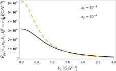
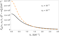
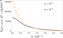
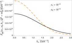
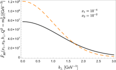
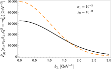
Figure 5: The distribution $\tilde{F}_{gg}(x_{1},x_{2},b_{\perp},Q^{2}=m_{H}^{2})$ evaluated for three pairs of $x_{1}$ and $x_{2}$ and depending on $b_{\perp}$. Double PDF calculations are displayed with (full lines) and without (dashed lines) Melosh operators. Upper panels for the HP model and lower panel for the HO one.

However, given the complicated structure of Eq. (105), it is non trivial to single out their effects, since they mix with the proton wave function. In order to determine to which extent their effects on dPDFs are independent of the chosen hadronic model, we compare dPDF calculations performed within the HO and the HP models and build appropriate ratios in order to highlight relativistic effects alone.

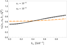
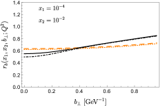
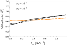
Figure 6: The ratio in Eq. (108) evaluated for digluon distribution as a function of $b_{\perp}$ for three pairs of values of $x_{1}$ and $x_{2}$. Black lines stand for dPDF calculations within the HP model, at $Q^{2}=m_{H}^{2}$ (full) and at $Q^{2}=4m_{c}^{2}$ (dot-dashed). Orange lines stand for dPDF computed within the HO model, at $Q^{2}=m_{H}^{2}$ (dashed) and at $Q^{2}=4m_{c}^{2}$ (dotted).

In Fig. 5 we present the double gluon distribution in coordinate space, $\tilde{F}_{gg}(x_{1},x_{2},b_{\perp},Q^{2}=m_{H}^{2})$, evaluated in different configurations of $x_{1}$ and $x_{2}$, including (black full lines) and neglecting (orange dashed lines) Melosh operators within different hadronic models, the HP in the upper panels and the HO in the lower ones. Results are consistent with those of Ref. [12], where only valence quark dPDFs have been evaluated at the low hadronic scale of the models. We observe in the plots that there exists a value of $b_{0}\sim 1.5$ Ge$\mbox{V}^{-1}$, which slightly depends upon the kinematics and the hadronic model used in the calculations, such that the inclusion of Melosh operators strongly decrease dPDFs for $b_{\perp}<b_{0}$ and slightly increase them for $b_{\perp}>b_{0}$. It is worth noticing that Melosh operators reduce to the identity for $k_{\perp}=0$, so that dPDFs with and without Melosh coincide in this limit. Since the latter condition corresponds to an integral of dPDFs over $d^{2}b_{\perp}$, it follows that dPDFs with and without Melosh are normalized to the same number. The digluon distributions in Fig. 5 show a marked dependence on the specific proton wave function built-in the CQMs. It is therefore instructive to present the ratio:

$$r_{b}(x_{1},x_{2},b_{\perp},Q^{2})={\tilde{F}_{gg}(x_{1},x_{,}b_{\perp},Q^{2})\over\tilde{F}_{gg}^{NM}(x_{1},x_{2},b_{\perp},Q^{2})}~{},$$ (108)

where we indicate with $\tilde{F}^{NM}_{gg}(x_{1},x_{2},b_{\perp},Q^{2})$ the dPDFs in Eq. (105) evaluated neglecting Melosh operators. The ratio in Eq. (108) is shown in Fig. 6 with calculations performed within the HP model at the final scales $Q^{2}=m_{H}^{2}$ (full lines) and $Q^{2}=4m_{c}^{2}$ (dot-dashed lines), and the HO model at the final scales $Q^{2}=m_{H}^{2}$ (dashed lines) and $Q^{2}=4m_{c}^{2}$ (dotted lines) in three configurations of $x_{1}$ and $x_{2}$. As one can see, up to $b_{\perp}<b_{0}$, Melosh operators induce a sizeable reduction of dPDFs which is almost a kinematical and scale independent effect. These conclusions hold for both the considered CQMs, which give rather close results. It is also interesting to study the impact of Melosh rotations directly on experimental related observables, such as $\sigma_{eff}$. We first consider the production of double $J/\Psi$ via DPS at the LHC. Calculations are performed in the rapidity range $|y|<1.2$ for ATLAS and CMS kinematics and $2<y<4.5$ for the LHCb one. The calculation of $\sigma_{eff}$ is performed via digluon distribution evaluated at $Q^{2}=4m_{c}^{2}$. In both these rapidity ranges, the involved parton momenta are quite small and we found that $\sigma_{eff}$ is nearly constant. For this reason we just quote the averaged results in Tab. 5. The inclusion of Melosh operators determines an increase in $\sigma_{eff}$ by almost $60\%$, whereas there is only a slight dependence on the chosen hadronic model. Then we consider double Higgs production via DPS in the same kinematic range. In this case, the digluon distribution is evaluated at $Q^{2}=m_{H}^{2}$. The results for $\sigma_{eff}$, as a function of final state particle rapidities, are shown in Figs. 7 and 8. We note that $\sigma_{eff}$ is almost constant in the central rapidity region, as already observed at $Q^{2}=4m_{c}^{2}$. However, for $Q^{2}=m_{H}^{2}$ in LHCb kinematics, the involved $x_{i}$ are substantially higher with respect to those addressed in the $Q^{2}=4m_{c}^{2}$ case and $\sigma_{eff}$ starts to show a non trivial $x$ dependence. From this plots it is clear that the production of heavy particles in the forward rapidity region represents a way to access the kinematic region where longitudinal correlation are the strongest. For both the considered final scales, the inclusion of Melosh operators increase the value of $\sigma_{eff}$, as they act to reduce the size of dPDFs at small $b_{\perp}$, as shown in Fig 5.

Kinematics	HO model		HP model
$Q^{2}=4m_{c}^{2}$	$\sigma_{eff}$ [mb]	$\sigma_{eff}^{NM}$ [mb]	$\sigma_{eff}$ [mb]	$\sigma_{eff}^{NM}$ [mb]
$|y|<1.2$	23.5	13.7	21.0	12.4
$2<y<4.5$	23.6	13.9	21.1	12.6

Table 5: Calculations of $\sigma_{eff}$ in the relevant experimental rapidity range of the process $pp\rightarrow J/\Psi J/\Psi X$. Results are presented for digluon distribution evaluated at $Q^{2}=4m_{c}^{2}$ and obtained within the HO and HP models, including and neglecting Melosh operators.

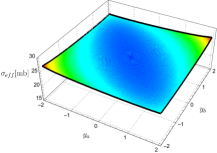
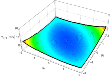
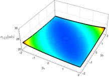
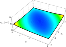
Figure 7: Effective cross section for the process $pp\rightarrow HHX$ as a function of Higgs bosons rapidities, $y_{a}$ and $y_{b}$, respectively in the central rapidity region. $\sigma_{eff}$ has been evaluated by using digluon distributions at the scale $Q^{2}=m_{H}^{2}$. In the upper panels results are shown within the HO model with (left) and without (right) Melosh operators. In the lower panels results are shown for the HP model with (left) and without (right) Melosh operators.

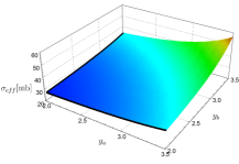
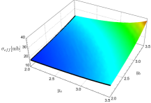
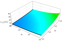
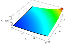
Figure 8: The same as in Fig. 7 but in the forward rapidity region.

The above results are similar, in quality, to that discussed in Ref. [58]. In order to further explore the role of Melosh operators in $\sigma_{eff}$, we consider the following ratio [12]:

$$r_{\sigma}(x_{1},x_{2})=\dfrac{\sigma_{eff}(x_{1},x_{2})}{\sigma^{NM}_{eff}(x_{1},x_{2})}~{},$$ (109)

where in the denominator the effective cross section has been evaluated by means of gluon dPDFs calculated without Melosh rotations. Results of numerical calculations are presented in Fig. 9 for three fixed typical values of $x_{1}$. Such a ratio shows a very weak dependence on $x$ and the chosen model, and a weak dependence on the hard scale. Moreover its numerical value is found to be quite close to that obtained with valence quarks dPDFs evaluated at the hadronic scale of models described in Ref. [12]. It is interesting to note that Melosh’s effects on $\sigma_{eff}$ by far exceed the dependence induced by using different hadronic models.

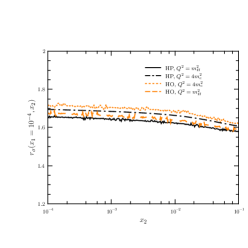
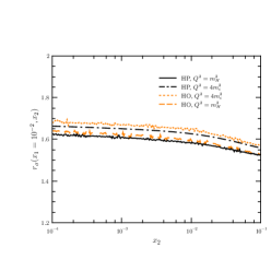
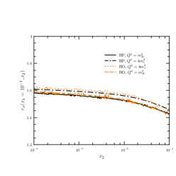
Figure 9: The ratio in Eq. (109) as a function of $x_{2}$ evaluated at fixed $x_{1}=10^{-4}$ (left panel), $x_{1}=10^{-2}$ (central panel) and $x_{1}=10^{-1}$ (right panel). This quantity has been calculated via the digluon distribution computed within the HP (full line) and the HO (dashed line) models at $Q^{2}=m_{H}^{2}$. The same quantity is shown within the HP (dot-dashed line) and the HO (dotted line) models at $Q^{2}=4m_{c}^{2}$.

As already discussed, Melosh operators encode $x-k_{\perp}$ correlations which guarantee the frame independence of the Light-Front wave function, an essential property which dPDFs must satisfy too. As previously shown above, Melosh effects on dPDF calculations are rather independent with respect to the adopted CQM, see Fig. 6 and Ref. [12]. Moreover, by comparing Figs. 6 and 9 with the corresponding Figs. 7 and 8 of Ref. [12], one may notice that such effects are also rather independent on the flavor of the active partons. In addition, as shown in Figs. 6,9, Melosh effects mildly depend on typical scales involved in the hard scatterings, either the $J/\Psi$ or the Higgs mass in the present analysis. These features suggest that one may study the functional form of these $x-k_{\perp}$ correlations which can then be used to inspire dPDFs phenomenological models. For this purpose we define the ratio $R$ between digluon PDFs calculated within CQM in a fully LF calculation and its approximation obtained neglecting Melosh operators:

$$R(x_{1},x_{2},k_{\perp})={F_{gg}(x_{1},x_{2},k_{\perp},Q^{2})\over F_{gg}^{NM}(x_{1},x_{2},k_{\perp},Q^{2})}~{}.$$ (110)

Such a ratio is built in order to suppress dynamical effects encoded in the chosen hadronic wave function. In fact, since we are interested in $x-k_{\perp}$ correlations induced only by Melosh operators, we have evaluated the ratio in Eq. (110) within the only model which does not include any additional $x-k_{\perp}$ correlation generated by its wave function, i.e. the HO model [9, 12].

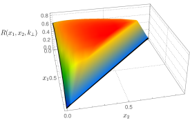
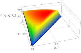
Figure 10: The ratio $R_{gg}(x_{1},x_{2},k_{\perp})$ evaluated within the HO model at the final scale $Q^{2}=m_{H}^{2}$. Left panel for $k_{\perp}=0.15$ GeV. Right panel for $k_{\perp}=1.97$ GeV.

We display in Fig. 10 the ratio $R(x_{1},x_{2},k_{\perp})$ for two representative values of $k_{\perp}$ as a function of $x_{1}$ and $x_{2}$. We found that a suitable parametrization in $x_{1}-x_{2}$ space, able to describe the ratio $R$ at fixed $k_{\perp}$, is the following one:

$$R(x_{1},x_{2},k_{\perp}) =w(k_{\perp})(x_{1}x_{2})^{t(k_{\perp})}(1-x_{1}-x_{2})^{|x_{1}-x_{2}|e(k_{\perp})}e^{-(1-x_{1}-x_{2})h(k_{\perp})}~{}.$$ (111)

The parameter $w$ controls the overall normalization of $R$, $t$ its small-$x$ behaviour. The additional parameter $e$ and $h$ control its behaviour on the $x_{1}+x_{2}=1$ boundary. Such a functional form goes beyond the standard factorized ansatz often used for dPDFs. By using the functional form in Eq. (111), we perform a series of fit of $R(x_{1},x_{2},k_{\perp})$ at fixed values of $k_{\perp}$. This procedure gives us access to the $k_{\perp}$ dependence of the parameters which is displayed in Fig. 11. Then, the $k_{\perp}$ dependence is interpolated by a fourth order polynomial of the type:

$$i(k_{\perp})=d_{i}+a_{i}k_{\perp}^{2}+b_{i}k_{\perp}^{3}+c_{i}k_{\perp}^{4}~{},\;\;i=\{w,e,t,h\},$$ (112)

involving four parameters for each $i$. For $k_{\perp}=0$ Melosh operators reduce to unity, $R(x_{1},x_{2},k_{\perp}=0)=1$, and therefore $e(k_{\perp}=0)=h(k_{\perp}=0)=t(k_{\perp}=0)=0$. The latter condition is fulfilled by setting $d_{e}=d_{h}=d_{t}=0$ and $d_{w}=1$ which are held fixed at those values during the fit. The corresponding results are displayed as solid lines in Fig. 11 and the best fit parameters are reported in Table 6. It is worth noticing that $w$ is compatible with unity and that $t$ is compatible with zero: Melosh operators mainly affect the behaviour of the ratio on the kinematic boundary. The dampening on the boundary is increasingly pronounced as $k_{\perp}$ increases. The obtained parametrization reproduces with good accuracy (at the percent level) the ratio $R(x_{1},x_{2},k_{\perp})$ calculated within the HO model. Additionally, its investigation at different scales, reveals that is substantially scale independent.

Figure 11: Symbols indicate the values of the parameters $w,e,t,h$ obtained by fitting the ratio R with Eq. (111) for fixed values of $k_{\perp}$. Lines indicate fit to these points obtained by using the functional form Eq. (112).

$i$	$a_{i}$	$b_{i}$	$c_{i}$	$d_{i}$
$w$	-0.202	0.146	-0.019	1
$e$	0.369	0.019	0.033	0
$t$	0.021	-0.012	0.002	0
$h$	-0.019	0.202	-0.043	0

Table 6: Values of the coefficients in the parametrizations in Eq. (112) as returned by the fit to the $k_{\perp}$ dependence of the ratio Eq. (110) evaluated within the HO model. The $d_{i}$ values are held fixed during the fit.

6 Conclusions

In the present analysis we have investigated to which extent information on the partonic proton structure, complementary to that obtained via other parton distributions, can be accessed via dPDFs. In particular we have focused our attention on the connection between the mean transverse partonic distance between two partons and $\sigma_{eff}$. We have discussed how this relation is modified when correlation of perturbative and non-perturbative origin are included in the calculation. In the former we have considered perturbative correlations induced by the so called splitting term in dPDF evolution. In the latter we have considered non perturbative correlation beyond the factorized ansatz for dPDFs. We proved that also in these two cases, the mean value of $\sigma_{eff}$ provides new indications on the structure of the proton in the non perturbative regime of QCD, again indicating dPDFs as a valuable tool to investigate partonic longitudinal and transverse correlations. In the last part of this work we took advantage of CQM calculations of dPDFs within the Light-Front relativistic approach, to study model independent correlations between $x_{1},x_{2}$ and $k_{\perp}$ induced by the so called Melosh operators. We have investigated their effects on the digluon dPDF, perturbatively obtained at high momentum scales relevant for DPS studies at the LHC. We have shown that Melosh operators produce a non-negligible reduction of dPDFs and generate, model independent, $x_{i}-k_{\perp}$ correlations on the kinematic boundary.

References

- [1] N. Paver and D. Treleani, Nuovo Cim. A 70, 215 (1982).
- [2] T. Sjostrand and M. van Zijl, Phys. Lett. B 188 (1987) 149; Phys. Rev. D 36 (1987) 2019.
- [3] T. Kasemets and S. Scopetta, arXiv:1712.02884 [hep-ph].
- [4] C. Goebel, F. Halzen and D. M. Scott, Phys. Rev. D 22 (1980) 2789.
- [5] M. Mekhfi, Phys. Rev. D 32 (1985) 2371.
-
[6]
M. Diehl and A. Schafer,
Phys. Lett. B 698, 389 (2011);
M. Diehl, D. Ostermeier and A. Schafer JHEP 03, 089 (2012). - [7] G. Calucci and D. Treleani, Phys. Rev. D 60, 054023 (1999)
- [8] H. M. Chang, A. V. Manohar and W. J. Waalewijn, Phys. Rev. D 87, no. 3, 034009 (2013)
- [9] M. Rinaldi, S. Scopetta and V. Vento, Phys. Rev. D 87, 114021 (2013)
- [10] W. Broniowski, E. Ruiz Arriola and K. Golec-Biernat, Few Body Syst. 57, no. 6, 405 (2016).
- [11] M. Rinaldi, S. Scopetta, M. Traini and V. Vento, JHEP 12, 028 (2014)
- [12] M. Rinaldi and F. A. Ceccopieri, Phys. Rev. D 95, no. 3, 034040 (2017)
- [13] M. Rinaldi, S. Scopetta, M. Traini and V. Vento, Eur. Phys. J. C 78, no. 9, 781 (2018)
- [14] S. Cotogno, T. Kasemets and M. Myska, arXiv:1809.09024 [hep-ph].
- [15] M. G. Echevarria, T. Kasemets, P. J. Mulders and C. Pisano, JHEP 04, 034 (2015)
- [16] M. Diehl and T. Kasemets, JHEP 05, 150 (2013)
- [17] T. Kasemets and M. Diehl, JHEP 01 (2013) 121.
- [18] G. S. Bali et al., arXiv:1807.03073 [hep-lat].
- [19] M. Aaboud et al. [ATLAS Collaboration], JHEP 11, 110 (2016).
- [20] R. Aaij et al. [LHCb Collaboration], JHEP 06 (2017) 047 Erratum: [JHEP 10 (2017) 068].
- [21] S. Chatrchyan et al. [CMS Collaboration], JHEP 03, 032 (2014)
- [22] A. M. Sirunyan et al. [CMS Collaboration], JHEP 02, 032 (2018)
- [23] M. Aaboud et al. [ATLAS Collaboration], Eur. Phys. J. C 77, no. 2, 76 (2017)
- [24] J. P. Lansberg and H. S. Shao, Phys. Lett. B 751, 479 (2015)
- [25] M. Rinaldi and F. A. Ceccopieri, Phys. Rev. D 97 (2018) no.7, 071501
- [26] A. M. Snigirev, Phys. Rev. D 68, 114012 (2003).
- [27] F. A. Ceccopieri, Phys. Lett. B 697 (2011) 482.
-
[28]
B. Blok, , Y. Dokshitzer, L. Frankfurt and M. Strikman,
Phys. Rev. D 83 (2011) 071501;
Eur. Phys. J. C 72, 1963 (2012); Eur. Phys. J. C 74, 2926 (2014). - [29] J. R. Gaunt and W. J. Stirling, JHEP 03, 005 (2010).
- [30] J. R. Gaunt, R. Maciula and A. Szczurek, Phys. Rev. D 90, no. 5, 054017 (2014)
- [31] D. Treleani and G. Calucci, arXiv:1808.02337 [hep-ph].
- [32] M. G. Ryskin and A. M. Snigirev, Phys. Rev. D 83 (2011) 114047
- [33] V. P. Shelest, A. M. Snigirev and G. M. Zinovev, Phys. Lett. 113B, 325 (1982).
- [34] R. Kirschner, Phys. Lett. 84B, 266 (1979).
- [35] V. L. Korotkikh and A. M. Snigirev, Phys. Lett. B 594, 171 (2004)
- [36] T. Kasemets and P. J. Mulders, Phys. Rev. D 91, 014015 (2015)
- [37] K. Golec-Biernat et al., Phys. Lett. B 750 (2015) 559
- [38] K. Golec-Biernat and E. Lewandowska, Phys. Rev. D 90 (2014) no.1, 014032
- [39] I. Schmidt and M. Siddikov, arXiv:1801.09974 [hep-ph].
- [40] E. Elias, K. Golec-Biernat and A. M. Stasto, JHEP 01 (2018) 141
- [41] M. Diehl, J. R. Gaunt, D. Ostermeier, P. Ploessl and A. Schafer, JHEP 01 (2016) 076
- [42] A. V. Manohar and W. J. Waalewijn, Phys. Rev. D 85, 114009 (2012)
- [43] J. R. Gaunt and W. J. Stirling, JHEP 06 (2011) 048
- [44] M. Diehl, T. Kasemets and S. Keane, JHEP 05, 118 (2014)
- [45] A. M. Snigirev, N. A. Snigireva and G. M. Zinovjev, Phys. Rev. D 90, no. 1, 014015 (2014)
- [46] M. Rinaldi, S. Scopetta, M. C. Traini and V. Vento, JHEP 10, 063 (2016)
- [47] V. M. Abazov et al. [D0 Collaboration], Phys. Rev. D 90, no. 11, 111101 (2014)
- [48] J. P. Lansberg, H. S. Shao, N. Yamanaka and Y. J. Zhang, arXiv:1906.10049 [hep-ph].
- [49] J. R. Gaunt, JHEP 07 (2014) 110.
- [50] M. Diehl, J. R. Gaunt and K. Schonwald, JHEP 06, 083 (2017)
- [51] M. Diehl and R. Nagar, arXiv:1812.09509 [hep-ph].
- [52] M. G. A. Buffing, M. Diehl and T. Kasemets, JHEP 01, 044 (2018)
- [53] F. A. Ceccopieri, Phys. Lett. B 734 (2014) 79
- [54] P. Faccioli, M. Traini and V. Vento, Nucl. Phys. A 656 (1999) 400 .
- [55] M. M. Giannini, Rept. Prog. Phys. 54, 453 (1991).
- [56] M. Diehl, P. Ploessl and A. Schafer, arXiv:1811.00289 [hep-ph].
- [57] F. A. Ceccopieri, M. Rinaldi and S. Scopetta, Phys. Rev. D 95 (2017) no.11, 114030
- [58] M. Rinaldi, S. Scopetta, M. Traini and V. Vento, Phys. Lett. B 752, 40 (2016)
- [59] D. Treleani, Phys. Rev. D 76 (2007) 076006
- [60] J. R. Gaunt, JHEP 01 (2013) 042.
- [61] L. Frankfurt and M. Strikman, Phys. Rev. D 66, 031502 (2002)
- [62] M. Traini, M. Rinaldi, S. Scopetta and V. Vento, Phys. Lett. B 768, 270 (2017)
- [63] P. A. M. Dirac, Rev. Mod. Phys. 21 (1949) 392 .
- [64] B. D. Keister and W. N. Polyzou, Adv. Nucl. Phys. 20, 225 (1991).
- [65] S. J. Brodsky, H. C. Pauli and S. S. Pinsky, Phys. Rept. 301, 299 (1998)
- [66] G. P. Lepage and S. J. Brodsky, Phys. Rev. D 22, 2157 (1980).
- [67] S. Boffi, B. Pasquini and M. Traini, Nucl. Phys. B 649, 243 (2003);
- [68] B. Pasquini, M. Traini and S. Boffi, Phys. Rev. D 71, 034022 (2005).
- [69] B. Pasquini, S. Cazzaniga and S. Boffi, Phys. Rev. D 78, 034025 (2008)
- [70] M. Traini, Phys. Rev. D 89, no. 3, 034021 (2014).
- [71] H. J. Melosh, Phys. Rev. D 9, 1095 (1974).
- [72] V. M. Abazov et al. [D0 Collaboration], Phys. Rev. Lett. 116, no. 8, 082002 (2016)
- [73] J. P. Lansberg and H. S. Shao, JHEP 10, 153 (2016)
- [74] J. P. Lansberg, H. S. Shao and N. Yamanaka, Phys. Lett. B 781, 485 (2018)
- [75] R. Aaij et al. [LHCb Collaboration], JHEP 07, 052 (2016)