Abstract

Models explaining dark matter typically include interactions with charged scalar and fermion fields. The Infra-Red (IR) finiteness of thermal field theories of charged fermions (fermionic QED) has been proven to all orders in perturbation theory. Here we reexamine the IR behaviour of charged scalar theories at finite temperature. Using the method of Grammer and Yennie, we identify and factorise the infra-red divergences to all orders in perturbation theory. The inclusion of IR finite pieces arising from the 4-point interaction terms of scalars with photon fields is key to the exponentiation. We use this in a companion paper to prove the IR finiteness of the corresponding thermal theory which is of relevance in dark matter calculations.

PACS: 11.10.−z, 11.10.Wx, 11.15.−q, 31.15.Md

1 Introduction

At zero temperature, Bloch and Nordsieck [1] were among the first to study the infra-red (IR) behaviour of fermionic QED. Later, it was shown [2] that the cross section for the bremsstrahlung of very low energy quanta in elementary particle collisions has an IR divergence:

$$\sigma_{\rm brems}=\frac{\sigma_{0}}{k}+\sigma_{1}+k\sigma_{2}+\ldots~{},$$ (1)

where $k$ is the energy of the photon and $\sigma_{j}$ have appropriate dimensions. It was further shown that $\sigma_{0}$ and $\sigma_{1}$ can be calculated from the corresponding elastic amplitude for both scalar and spinor cases at the leading order in perturbation theory, calculated up to ${\mathcal{O}}(k)$. This was later extended [3] for pure fermionic QED where it was shown that the (logarithmic) IR divergences cancel to all orders (rendering the total cross section IR finite) when both virtual and real photon emission corrections are included. Such soft real emissions need to be included due to finite detector resolution since they cannot be distinguished from the virtual lower order process. Some of the technical shortcomings of Ref. [3] such as translational and gauge-invariance were addressed in a subsequent paper by Grammer and Yennie [4].

Many clarifications and simplifications occurred over the next decades, including [5] the question about whether a charge particle exists relativistically due to the IR structure of gauge theories where the Green functions for charged matter have no poles but a branch cut. This implies a soft cloud always surrounds each physical charge. This question was addressed (positively) in Ref. [6, 7] where they used velocity-superselection rules inspired by heavy quark effective theory for abelian theories to obtain on-shell Green’s functions that are IR finite to all orders in perturbation theory. Specifically, they used scalar QED for simplicity, since Low [2] had shown that the electron spin structure does not affect the IR divergence as long as the matter fields are massive. (The spin structure of massless QED makes its asymptotic dynamics richer; for instance, collinear divergences turn on.) Scalar QED has also been studied recently [8] in the context of its asymptotic symmetries and relation to Weinberg’s soft photon theorem.

Many papers have also addressed the IR finite remainder in such scalar theories. For instance, in Refs. [9, 10, 11], the factorisation and exponentiation of IR divergences is shown in a translation and gauge-invariant way, using order-by-order agreement with Operator Product Expansion (OPE) before summation and by requiring that the exponentiation of all factorisable parts is done before the integrations are carried out. Then the IR finite remainder is defined in terms of correlations with respect to the photon momenta in the integrands. This involves an all order generalisation of Low’s theorem and also includes a calculation of both soft and hard photon contributions.

In the case of thermal field theory, there are additional linear divergences owing to the nature of the thermal photon propagator. The infra-red finiteness of such thermal QED with purely charged fermions has been shown [12, 13] to all orders in the theory. In particular, both absorption and emission of photons with respect to the heat bath are required [12, 14] in order to cancel the linear divergences as well as the logarithmic subdivergences.

In the first of this set of two papers we address the proof of the infrared finiteness, to all orders, of a thermal field theory of pure charged scalars, referred to as scalar QED. In the second paper, we apply these results, and the earlier results on the IR finiteness of thermal fermionic QED, to address the issue of IR finiteness of of thermal models of dark matter, thereby extending the results obtained in Ref. [15] at NLO to all orders. The analysis is an extension of that presented in Ref. [12] which was based on the approach developed by Grammer and Yennie (GY) [4] and is motivated by the results of Ref. [15]. The crux of this paper is the identification of the correct set of terms that allows the factorisation and exponentiation of the IR divergent terms to all orders for thermal scalar fields.

In contrast to fermionic QED, we now have not only the 3-point scalar-photon-scalar vertex, but also 4-point (2-scalar-2-photon) ones. These contribute through both seagull and tadpole diagrams; see vertex diagrams in Appendix A. While the result we obtain is similar to that obtained in the usual fermionic QED, the inclusion of the seagull and tadpole diagrams give rise to additional terms that are essential in order to achieve the exponentiation and cancellation of IR divergent terms between real and virtual contributions.

In the next paper, Paper II, we apply our results to show the IR finiteness of the corresponding thermal field theory of dark matter to all orders. This result is, thus, a generalisation of Ref. [12] to include both charged fermions and scalars. Again, the key fact used in the proof is that both photon absorption and emission diagrams are required to cancel the linear sub-divergences. As mentioned earlier, this was also noticed in the NLO calculation in Ref. [15], where the finite term has also been calculated to NLO.

In Section 2, we briefly review the propagator and vertex structure of the relevant thermal field theory; details are given in Appendix A. We also review the approach of Grammer and Yennie (GY) to address the IR behaviour of such field theories. In Section 3, we analyse the photon–scalar interactions using the approach motivated by GY: by rearranging the polarisation sums of the inserted virtual photons into so-called $K$-photon and $G$-photon parts (see Eq. 4). This was used by GY to establish the IR finiteness of fermionic QED to all orders. As in the case of fermionic QED, the $K$-photon contributions are divergent; however, in scalar QED, they can be factorised and exponentiated only on inclusion of the additional vertices. In particular, the ${\mathcal{O}}(k^{2})$ IR finite contribution from the tadpole diagrams cancels a similar contribution from the 3-particle interaction terms and enables the factorisation. As far as we are aware, this observation of the need for inclusion of the IR finite tadpole contributions in order to achieve the factorisation and subsequent exponentiation of the IR divergent parts, has not been pointed out in the literature before. The $G$-photon contributions are finite, again, as was shown to be the case for fermionic QED. Proof of IR finiteness of the $G$-photon insertions is non-trivial due to the presence of both 4-point vertices as well as thermal indices and is the second main contribution of this work. In Section 3, the corresponding analysis for insertion of real photons is also considered. A similar rearrangement of the polarisation sums of real photons into $\widetilde{K}$ and $\widetilde{G}$ enables the IR divergent parts to be collected into the $\widetilde{K}$ contribution. We show that the IR divergent parts will cancel between the virtual and real diagrams, that is, between the $K$ and $\widetilde{K}$ contributions, when they are added, order by order, in the theory. This is achieved only when both real photon emission into, and absorption from, the heat bath is taken into account. This establishes the infrared finiteness to all orders for scalar thermal QED. We end with some remarks and discussion in Section 4. Many technical details are relegated to the appendices.

Appendix A lists the relevant Feynman rules while Appendix B lists some useful generalised Feynman identities of use in the thermal field theoretic analysis. The details of the calculation for the insertion of a virtual $K$ photon into a lower order graph is found in Appendix C where it is shown that the total contribution from all possible virtual $K$ photon insertions into an $n^{\rm th}$ order graph is a single term proportional to the lower order matrix element itself (and is also IR divergent). Details of the result for the insertion of a virtual $G$ photon in all possible ways into an $n^{\rm th}$ order graph is found in Appendix D; it is shown that all such virtual $G$ photon contributions are IR finite.

2 Real-time formulation of thermal field theory

We review briefly the real-time formulation of thermal (scalar and photon) fields in equilibrium with a heat bath at temperature $T$. In the case of such a thermal field theory, there is an additional complication which can be understood in a real-time formulation [16] where the integration in the complex time plane is over a contour that includes the temperature, chosen so that correct thermal averages of the $S$-matrix elements [17] are obtained. The fields satisfy periodic boundary conditions,

$$\varphi(t_{0})=\varphi(t_{0}-i\beta)~{},$$ (2)

where $\beta=1/T$, with $T$ being the temperature of the heat bath. This results in the well-known field-doubling, so that fields are of type-1 (physical) or type-2 (ghosts), with propagators acquiring $2\times 2$ matrix forms. Only type-1 fields can occur on external legs (as mandated by unitarity) while fields of both types can occur on internal legs, with the off-diagonal elements of the propagator allowing for conversion of one type into another.

Both scalar and photon field propagators assume matrix forms (see Appendix A for details) with the (11) and (22) terms having both $T=0$ and finite temperature contributions. In particular, the photon propagator corresponding to a momentum $k$ can be expressed (in the Feynman gauge) as,

$$i{\cal D}^{ab}_{\mu\nu}(k) =-ig_{\mu\nu}\,D^{ab}(k)~{},$$ (3)

where the information on the field type is contained in $D^{ab}(k)$; see Appendix A for its definition.

Finally, the vertices, both 3-point and 4-point ones, are modified in the thermal theory. Details are again in Appendix A; we only note here that all the fields at a given vertex must be of the same type.

2.1 The GY approach to study the IR behaviour

Several methods can be adopted to prove all-order finiteness. For example, one may consider propagators dressed with arbitrary coherent states. We shall, instead, adopt a simpler method that lends itself more readily to an understanding of the issues involved. The approach of GY, which we use here, addressed the IR finiteness of fermionic QED at zero temperature, and we extend this to a theory of charged scalars in contact with a heat bath. GY started with an $n^{\rm th}$-order graph with $n$ photon-fermion vertices and considered the effect of adding an additional real or virtual photon to it. Since the photon is a boson, all symmetric permutations, i.e., all possible insertions, must be considered. In particular, for the virtual photon insertion, they found it useful to express the photon propagator as,

$$-i\frac{g_{\mu{\nu}}}{k^{2}+i\epsilon} =\frac{-i}{k^{2}+i\epsilon}\,\left[\left(g_{\mu\nu}-b_{k}(p_{f},p_{i})k_{\mu}k_{\nu}\right)+\left(b_{k}(p_{f},p_{i})k_{\mu}k_{\nu}\right)\right]~{},$$

$$\equiv\frac{-i}{k^{2}+i\epsilon}\,\left[G_{\mu\nu}+K_{\mu\nu}\right]~{}.$$ (4)

Here, $b_{k}$ depends on the momenta $p_{f}$, $p_{i}$, where the final and initial vertices are inserted (and also implicitly on the momentum $k$ of the inserted $(n+1)^{\rm th}$ photon), and is defined such that the so-called $G$-photon terms in the matrix element with $(n+1)$ photons are IR finite (in both the $T=0$ and $T\neq 0$ cases for fermionic QED) and the $K$-photon terms contain all the IR divergent terms:

$$b_{k}(p_{f},p_{i})=\frac{1}{2}\left[\frac{(2p_{f}-k)\cdot(2p_{i}-k)}{((p_{f}-k)^{2}-m^{2})((p_{i}-k)^{2}-m^{2})}+(k\leftrightarrow-k)\right]~{}.$$ (5)

Note that, on account of its $k$ dependence, $b_{k}$ does not represent a gauge transformation.

On expressing the $(n+1)^{\rm th}$ virtual photon contribution in this way, the $K$ photon contribution turns out to be proportional to the matrix element of the underlying graph with $n$-photon vertices and has a simple structure. The object of this paper is to obtain an analogous result for a theory of thermal charged scalars.

Note that the factor $g_{\mu\nu}$ occurs in all components of the thermal photon propagator, enabling a separation into $K$- and $G$-type photons, just as before, with the same definition for $b_{k}$ as in Eq. 5. We can therefore apply the technique of GY to the case of thermal fields in equilibrium with a heat bath at temperature $T$. There are two major differences in this case, firstly, that the relevant part of the thermal photon propagator is proportional to,

$$i{\cal{D}}^{ab}(k)\sim \left[\frac{i}{k^{2}+i\epsilon}\delta^{ab}\pm 2\pi\delta(k^{2})N(|k^{0}|)D^{ab}_{T}\right]~{},$$ (6)

where the first term corresponds to the $T=0$ contribution and the second to the finite temperature part. The bosonic number operator in the second term contributes an additional power of $k$ in the denominator in the soft limit, since

$$N(|k^{0}|)\equiv\frac{1}{\exp^{|k^{0}|/T}-1}\;\stackrel{{\scriptstyle k\to 0}}{{\longrightarrow}}\;\frac{T}{|k^{0}|}~{}.$$ (7)

Hence, it can be seen that the leading IR divergence in the finite temperature part is linear rather than logarithmic as was the case at zero temperature. Consequently, there is a residual logarithmic subdivergence that must also be shown to cancel at finite temperatures, thus making the generalisation to the thermal case non-trivial.

Secondly, it turns out that the inclusion of thermal matter fields adds another layer of complexity to the analysis, since not only is the propagator structure now different from the zero temperature case, but, in contrast to the case of fermions, the number operator corresponding to charged scalars is bosonic and hence can potentially give rise to divergences as well.

In summary, the major differences between this and the earlier works are as follows.

1. The scalar theory has additional vertices, including the 4-point seagull vertices; see Fig. 11 in Appendix A. This contributes additional terms to both the $K$ and $G$ photon insertions compared to the thermal theory with fermions only.

2. The thermal theory has additional field types; in particular, the thermal charged scalar legs add more complications compared to the results with thermal fermions.

We consider both modifications when analysing the IR behaviour of thermal scalar QED in the next section.

3 The IR behaviour of thermal scalar QED

In view of the discussion in the preceding section, we begin by considering pure scalar QED, discounting quartic scalar self-couplings. Thus, it behoves us to start with the fundamental hard scattering process here, viz. $\gamma^{(*)}+\phi^{(*)}\to\phi^{(*)}$ where any of the three lines could represent either an on-shell or an off-shell particle. Higher order contributions would arise from the inclusion of both virtual as well as soft real photons.

We begin by considering insertions on an $n$-photon graph with trilinear (scalar-scalar-photon) vertices alone so that the $n$ vertices imply $n$ scalar–photon interactions (with the understanding that both vertices of an internal line are counted). We will, subsequently, extend the analysis to graphs with an arbitrary admixture of 3-point and 4-point vertices.

The $(n)^{\rm th}$ order graph has $n$ trilinear vertices with $s$ vertices on the final scalar leg with 4-momentum $p^{\prime}$ and $r\,(=n-s)$ vertices on the initial scalar leg with 4-momentum $p$ (see Fig. 1). For reasons that will become clear later, these vertices are already symmetrised. The photons carry away momentum $l_{q},\,q=1,\cdots,s$, from the vertex $q$ on the $p^{\prime}$-leg and momentum $-t_{q},\,q=1,\cdots,r$, from the vertex $q$ on the $p$ leg. The notation is arbitrary since the momenta may be entering or leaving the vertex and the corresponding photon may be a real or virtual one.

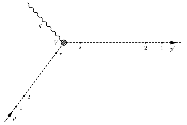
Figure 1: Schematic of an $n^{\rm th}$ order graph of $\gamma^{*}\phi\to\phi$, with $s$ vertices on the $p^{\prime}$ leg and $r$ on the $p$ leg, $r+s=n$. $V$ labels the special but arbitrary hard photon–scalar vertex.

Hence the momentum of the particle to the right of the $q^{\rm th}$ vertex on the $p$ leg is $(p+\textstyle\sum_{i=1}^{q}t_{i})$ while the momentum corresponding to the particle line to the left of the $q^{\rm th}$ vertex on the $p^{\prime}$ leg is $(p^{\prime}+\textstyle\sum_{i=1}^{q}l_{i})$.

In contrast to the fermionic case, which has only three-point vertices, scalar QED admits of 4-point vertices as well, so that an additional photon can be inserted at a new vertex (giving rise to a new 3-point vertex) or at an already existing 3-point vertex, thus converting it to a 4-point vertex. Thus the consideration of charged scalars requires consideration of both types of insertions. This is true for both real and virtual photon insertions.

We begin by considering insertion of an additional virtual photon. Adopting the expression of $g_{\mu\nu}$ in the photon propagator in terms of $K_{\mu\nu}$ and $G_{\mu\nu}$ (as in Eq. 4), we start with the insertion of virtual $K$-photons (which are expected to contain the IR divergent contributions) leaving the inclusion of the $G$-photons (expected to give IR finite contributions) until later.

3.1 Insertion of virtual $K$ photons

Consider the insertion of one of the virtual $K$ photon vertices, say $\mu$, on an external line. As per the Feynman rules listed in Appendix A, there can be two types of vertices, with one or two photon lines at each vertex, corresponding to 3-point or 4-point vertices respectively. (In addition, these fields carry a thermal index, $t_{a}(=1,2)$, depending on the field type at the $a^{\rm th}$ vertex). Hence, there are two types of $K$ photon insertions possible; one where the insertion is at a new vertex, forming a new 3-point vertex, or one where the $(n+1)^{\rm th}$ $K$ photon is inserted on an already existing vertex, thus forming a 4-point vertex. The total set of all possible insertions of the $(n+1)^{\rm th}$ $K$ photon on the $p^{\prime}$ line can be grouped into sets having the new $\mu$ vertex as a 3-point or 4-point vertex, as shown in Figs. 2 and 3 respectively. In contrast, note that only the set of graphs shown in Fig. 2 contributes if the $p^{\prime}$-leg is a fermion line.

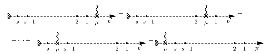
Figure 2: Set of $(s+1)$ diagrams showing all possible trilinear insertions of a virtual photon at vertex $\mu$ on the $p^{\prime}$ leg of a scalar/fermion.

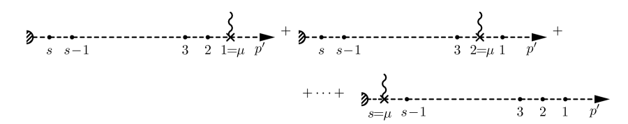
Figure 3: Set of $s$ diagrams showing all possible insertions of a virtual photon at vertex $\mu$ which is one of the already existing $s$ vertices on the $p^{\prime}$ leg of a scalar particle, thus giving rise to a 4-point vertex. Analogous diagrams for fermions do not exist.

It is convenient to group 3- and 4-point vertices to obtain “circled vertices”: for instance, consider the insertion of the $\mu$ vertex to the right of a generic vertex $q$ or at the vertex $q$. The corresponding two diagrams are shown in Fig. 4 and the contribution from the sum of these is shown in the figure as a circled vertex and denoted by ${}_{q}\mu$.

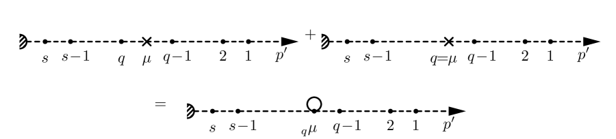
Figure 4: Combining the two possible sets of insertions (as in Figs. 2 and 3) of the $(n+1)^{\rm th}$ virtual $K$ photon at the vertex $\mu$ on the $p^{\prime}$ leg to give a single circled vertex, ${}_{q}\mu$; see text for details. The photon lines have been suppressed for clarity.

In the thermal case, the propagators contain more than just the $1/(P^{2}-m^{2})$ part and appear more complex. However, they satisfy generalised identities, analogous to the zero temperature case, as shown in Appendix B, which can be used to simplify and factor these contributions to obtain a similar result. Retaining only the $k_{\mu}$ factor in the $(b_{k}k_{\mu}k_{\nu})$ part of the $K$ photon propagator (the $k_{\nu}$ factor will be similarly included when the other vertex $\nu$ is inserted on the $p$ leg, and $b_{k}$ is an overall factor), and omitting the other terms in the photon propagator for clarity, we have (denoting a scalar propagator from the vertex $\mu_{b}$ of thermal type $t_{b}$ to the vertex $\mu_{a}$ having fields of thermal type $t_{a}$ as $i{\cal S}^{t_{a}t_{b}}(p^{\prime}+\sum_{i=1}^{q}l_{i},m)\equiv iS^{ab}_{p^{\prime}+\sum_{q}}\hbox{)}$,

$${\cal M}_{n+1}^{q~{}{\rm to~{}left~{}of~{}}\mu} =\begin{multlined}e^{s+1}(-1)^{\hbox{(}\sum_{i=1}^{s}t_{i}\hbox{)}+s}\cdots(-1)^{t_{\mu}+1}\left[S^{q-1,\mu}_{p^{\prime}+\sum_{q-1}}\times((2p^{\prime}+2\Sigma_{q-1}+k)\cdot k)\times\right.\\ \qquad\qquad\left.S^{\mu,q}_{p^{\prime}+\sum_{q-1}+k}\right]\left(2p^{\prime}+2\Sigma_{q-1}+2k+l_{q}\right)_{\mu_{q}}S^{q,q+1}_{p^{\prime}+\sum_{q}+k}\cdots~{},\end{multlined}e^{s+1}(-1)^{\hbox{(}\sum_{i=1}^{s}t_{i}\hbox{)}+s}\cdots(-1)^{t_{\mu}+1}\left[S^{q-1,\mu}_{p^{\prime}+\sum_{q-1}}\times((2p^{\prime}+2\Sigma_{q-1}+k)\cdot k)\times\right.\\ \qquad\qquad\left.S^{\mu,q}_{p^{\prime}+\sum_{q-1}+k}\right]\left(2p^{\prime}+2\Sigma_{q-1}+2k+l_{q}\right)_{\mu_{q}}S^{q,q+1}_{p^{\prime}+\sum_{q}+k}\cdots~{},$$

$$=e^{s+1}(-1)^{\hbox{(}\sum_{i=1}^{s}t_{i}\hbox{)}+s}\cdots\left[S^{q-1,q}_{p^{\prime}+\sum_{q-1}}\delta_{t_{\mu},t_{q}}-S^{q-1,q}_{p^{\prime}+\sum_{q-1}+k}\delta_{t_{\mu},t_{q-1}}\right]\cdots~{},$$ (9)

$${\cal M}_{n+1}^{q=\mu} =e^{s+1}(-1)^{\hbox{(}\sum_{i\neq q}^{s}t_{i}\hbox{)}+s-1}\cdots(-1)^{t_{\mu}+1}\left[S^{q-1,\mu}_{p^{\prime}+\sum_{q-1}}(-2k_{\mu_{q}})\delta_{t_{\mu},t_{q}}\times S^{q,q+1}_{p^{\prime}+\sum_{q}+k}\right]\cdots~{};$$

$$=e^{s+1}(-1)^{\hbox{(}\sum_{i=1}^{s}t_{i}\hbox{)}+s}\cdots\left[S^{q-1,q}_{p^{\prime}+\sum_{q-1}}\delta_{t_{\mu},t_{q}}(-2k_{\mu_{q}})S^{q,q+1}_{p^{\prime}+\sum_{q}+k}\right]\cdots~{}.$$ (10)

Here, $t_{i}(=1,2)$ denote the thermal indices of the inserted photons and $t_{\mu}$ is the thermal index of the inserted photon at the vertex $\mu$. Notice that all the thermal powers of $(-1)^{t_{i}+1}$ match and there is no sign ambiguity between the relative contributions of the two terms, which is independent of the thermal field type. Hence the two can be combined to give the total contribution to Fig. 4 as a difference of two terms, viz.,

$${\cal M}_{n+1}^{q\mu,{\rm tot}} =e^{s+1}(-1)^{\hbox{(}\sum_{i=1}^{s}t_{i}\hbox{)}+s}\cdots\left[S^{q-1,q}_{p^{\prime}+\sum_{q-1}}\delta_{t_{\mu},t_{q}}\left(2p^{\prime}+2\Sigma_{q-1}+l_{q}\right)_{\mu_{q}}\right.$$

$$\hskip 85.35826pt\left.-S^{q-1,q}_{p^{\prime}+\sum_{q-1}+k}\delta_{t_{\mu},t_{q-1}}\left(2p^{\prime}+2\Sigma_{q-1}+2k+l_{q}\right)_{\mu_{q}}\right]S^{q,q+1}_{p^{\prime}+\sum_{q}+k}\cdots~{}.$$ (11)

This is the thermal generalisation of the corresponding result obtained by GY for the fermionic case at $T=0$. This combination of differences of terms from $K$ photon insertion helps in pair-wise cancellation and hence simplification and factorisation of the IR divergent part even at finite temperature. Note that due to the absence of 4-point vertices, the corresponding thermal result for the insertion of a thermal virtual $K$ photon into a fermion line was much simpler [12]:

$${\cal M}_{n+1}^{q\mu,{\rm fermion}} =e^{s+1}(-1)^{\hbox{(}\sum_{i=1}^{s}t_{i}\hbox{)}+s}\left[S^{q-1,q}_{p^{\prime}+\sum_{q-1}}\delta_{t_{\mu},t_{q}}-S^{q-1,q}_{p^{\prime}+\sum_{q-1}+k}\delta_{t_{\mu},t_{q-1}}\right]~{}S^{q,q+1}_{p^{\prime}+\sum_{q}+k}\cdots~{},$$ (12)

where the propagators are now fermionic. We now apply this simplification to all sets of diagrams. We have the following possibilities:

1. The inserted $K$ photon vertices are on different external lines, in-coming and out-going.

2. The two vertices of the inserted $K$ photon are on the same lines.

We will address them one by one.

3.1.1 $K$ photon insertions on different lines

The case where the vertices are on different lines is straightforward. Start with a lower order diagram that contains only 3-point vertices; we will relax this condition later. Consider the insertion of the $\mu$ vertex of the $(n+1)^{\rm th}$ $K$ photon in all possible ways on the $p^{\prime}$ leg. In terms of the circled vertices, these can be expressed in terms of the graphs shown in Fig. 5.

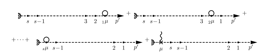
Figure 5: The graphs in Figs. 2 and 3 can be combined into the $s$ circled vertex graphs and an $(s+1)^{\rm th}$ graph with the inserted $\mu$ vertex to the left of all the other $s$ vertices on the $p^{\prime}$ leg, as shown above.

Since the relevant term in the $K$ photon propagator is $(b_{k}k_{\mu}k_{\nu})$, we compute the contribution to the part of the matrix element, ${\cal{M}}_{n+1}^{\mu,p^{\prime}{\rm leg}}$, from an insertion $\mu$ on the $p^{\prime}$ leg. The contribution from each of the first $s$ graphs in Fig. 5, retaining only the $k_{\mu}$ term in the photon propagator, and omitting overall constants including a factor of $e^{s+1}(-1)^{\hbox{(}\sum_{i=1}^{s}t_{i}\hbox{)}+s}$, can be written from inspecting the result in Eq. 11 (see the corresponding graphs in Fig. 4),

$${\cal{M}}_{n+1}^{\mu,p^{\prime},s} \propto \left\{0+\delta_{t_{\mu},t_{1}}(2p^{\prime}+l_{1})_{\mu_{1}}S^{t_{1},t_{2}}_{p^{\prime}+\sum_{1}+k}(2p^{\prime}+2\Sigma_{1}+2k+l_{2})_{\mu_{2}}\cdots(V)\cdots\right\}$$ (13)

$$+\left\{(2p^{\prime}+l_{1})_{\mu_{1}}\left[S^{t_{1},t_{2}}_{p^{\prime}+\sum_{1}}\delta_{t_{\mu},t_{2}}(2p^{\prime}+2\Sigma_{1}+l_{2})_{\mu_{2}}\right.\right.$$

$$\left.\left.-S^{t_{1},t_{2}}_{p^{\prime}+\sum_{1}+k}\delta_{t_{\mu},t_{1}}(2p^{\prime}+2\Sigma_{1}+2k+l_{2})_{\mu_{2}}\right]\cdots(V)\cdots\right\}$$

$$+\left\{\cdots\right\}$$

$$+\left\{(2p^{\prime}+l_{1})_{\mu_{1}}S^{t_{1},t_{2}}_{p^{\prime}+\sum_{1}}\cdots\left[S^{t_{s-1},t_{s}}_{p^{\prime}+\sum_{s-1}}\delta_{t_{\mu},t_{s}}(2p^{\prime}+2\Sigma_{s-1}+l_{s})_{\mu_{s}}\right.\right.$$

$$\left.\left.-S^{t_{s-1},t_{s}}_{p^{\prime}+\sum_{s-1}+k}\delta_{t_{\mu},t_{s-1}}(2p^{\prime}+2\Sigma_{s-1}+2k+l_{s})_{\mu_{s}}\right]\cdots(V)\cdots\right\}~{},$$

$$= \left\{0+M_{1}\right\}+\left\{M_{2}-M_{1}\right\}+\left\{\cdots\right\}+\left\{M_{s}-M_{s-1}\right\}~{}.$$

Here $(V)$ denotes the (arbitrary) vertex that separates the $p^{\prime}$ and $p$ legs, and the first term vanishes since $p^{\prime}$ is on-shell. It can be seen that the terms now cancel, just as happened in the $T=0$ case for GY, leaving only the last term, $M_{s}$. The contribution from the unpaired $(s+1)^{\rm th}$ term which is the last graph shown in Fig. 2 is

$${\cal{M}}_{n+1}^{\mu,p^{\prime},s+1} \propto(2p^{\prime}+l_{1})_{\mu_{1}}S^{t_{1},t_{2}}_{p^{\prime}+\sum_{1}}\cdots\left[S^{t_{s},t_{V}}_{p^{\prime}+\sum_{s}}\delta_{t_{\mu},t_{V}}-S^{t_{s},t_{V}}_{p^{\prime}+\sum_{s}+k}\delta_{t_{\mu},t_{s}}\right]\,(V)\cdots~{},$$

$$=\left\{M_{s+1}-M_{s}\right\}~{}.$$ (14)

Hence the second term of Eq. 14 cancels the contribution of the previous $s$ terms in Eq. 13, so that the total contribution from the insertion of the $\mu$ vertex of the $(n+1)^{\rm th}$ $K$ photon in all possible ways on the $p^{\prime}$ leg gives a contribution that is independent of the inserted momentum, $k$, as in the case with fermions. That is, the result of adding the contributions of inserting both A and B types of vertices in all possible ways on the $p^{\prime}$ leg is,

$${\cal{M}}_{n+1}^{\mu,p^{\prime},tot} \propto(2p^{\prime}+l_{1})_{\mu_{1}}S^{t_{1},t_{2}}_{p^{\prime}+\sum_{1}}\cdots S^{t_{s},t_{V}}_{p^{\prime}+\sum_{s}}\left[\delta_{t_{\mu},t_{V}}\right]\,(V)\cdots~{}.$$ (15)

Note the presence of the delta-function, $\delta_{t_{\mu},t_{V}}$, arising from matching the field types at the vertex. Since the hard photon is observable, $t_{V}=1$ and hence $t_{\mu}=1$ as well.

3.1.1.1 Inclusion of the 4-point vertex

The calculation can be extended to the case when there are both 3- and 4-point vertices in the $n$-photon graph. Graphs with the same number of photons rather than the same number of vertices are grouped together, so that the overall charge factors (powers of $\alpha$) are the same for the entire set of diagrams. Hence the corresponding $n$-photon graph may have fewer than $n$ vertices, and in fact will have $(m/2+(n-m))$ vertices if $m$ of the $n$ photons participate in a 4-point vertex. For such diagrams there is an additional constraint since it is obvious that the additional $(n+1)^{\rm th}$ photon cannot be added at an already existing 4-point vertex.

Two photons, say $l_{q}$ and $l_{r}$, are at vertex $q$. No more photons can be added at this vertex, and in fact, the vertex factor for this vertex is proportional to $g_{qr}\delta_{t_{q},t_{r}}$, with no momentum dependence. As before, any $q=\mu$ vertex (that is, the new photon forms a 4-point vertex) contributes a term with a factor $(-2k_{\mu_{q}})$ in the numerator which cancels a similar term from a 3-point $\mu$ vertex as shown in Fig. 4. The terms cancel diagram by diagram, similar to that shown in Eq. 13. The $g_{qr}\delta_{t_{q},t_{r}}$ factor gets carried along and does not spoil the re-grouping and cancelling of terms when an additional $(n+1)^{\rm th}$ $K$-photon vertex $\mu$ is added.

A similar result is obtained when the $\nu$ vertex of the virtual $K$ photon is inserted on the $p$ (distinct) leg, with pair-wise cancellations, leaving a single term containing $\delta_{t_{\nu},t_{V}}$. Putting back the factors of $b_{k}(p^{\prime},p)$ as well as the rest of the photon propagator, the total contribution from the insertion in all possible ways of an $(n+1)^{\rm th}$ $K$-photon (contributing a factor $(b_{k}(p^{\prime},p)k_{\mu}k_{\nu})$) into a set of graphs with $n$ photons containing an arbitrary number of 3- or 4-point vertices, is given by,

$${\cal M}^{p^{\prime}p,K\gamma}_{n+1} =-ie^{2}\int\frac{{\rm d}^{4}k}{(2\pi)^{4}}\,\delta_{t_{\mu},t_{V}}\,\delta_{t_{\nu},t_{V}}b_{k}(p^{\prime},p)D^{t_{\mu},t_{\nu}}(k)\times{\cal M}_{n}~{},$$ (16)

and hence is proportional to the lower order matrix element ${\cal M}_{n}$.

The major difference between the $T=0$ case and the thermal case is the presence of the thermal indices. Crucially, there are additional delta functions, $\delta_{t_{\mu},t_{V}}$ and $\delta_{t_{\nu},t_{V}}$, arising from matching the field types at the special (hard) scalar-photon vertex $V$. Since the hard photon is observable, $t_{V}=1$ so $t_{\mu}$, $t_{\nu}=1$ as well; hence the $K$ photon thermal propagator is constrained to be of type $D^{11}$ alone. This is a crucial requirement for the cancellation to occur between real and virtual photon contributions to the lower order diagram, as we shall see below.

3.1.2 Both $K$ photon insertions on the $p^{\prime}$ leg alone

The case where both vertices of the $(n+1)^{\rm th}$ $K$ photon are inserted on the $p^{\prime}$ leg is more complex due to the presence of a large number and type of diagrams as well as the presence of the additional 4-point vertices. While only seagull 4-point vertices contribute in the previous case (of independent insertions of $\mu$ and $\nu$ on different legs), tadpole diagrams also contribute when both vertices are inserted at the same point on the same leg. Double-counting is avoided by insisting that the $\mu$ vertex is always to the right of the $\nu$ vertex.

As before, the case with only 3-point vertices in the lower order graph is first considered; this condition is then relaxed to prove the general case. The diagrams obtained when the $(n+1)^{\rm th}$ $K$ photon is inserted in all possible ways can be grouped into sets labelled Set I, Set II, Set III, and Set IV, as shown in Figs. 6 to 9. While Set I (Fig. 6) has circled vertices at both $\mu$ and $\nu$ insertions, Set II (Fig. 7) has circled vertices only at $\mu$, with $\nu$ to the right of the special $V$ vertex. Set III (Fig. 8) has all 4-point vertex insertions at $\nu$, with $\mu$ immediately adjacent to $\nu$. Finally, Set IV (Fig. 9) is a set of ${}_{\nu}\mu$ circled vertices that includes all tadpole insertions, $\mu=\nu$, as shown in Fig. 10.

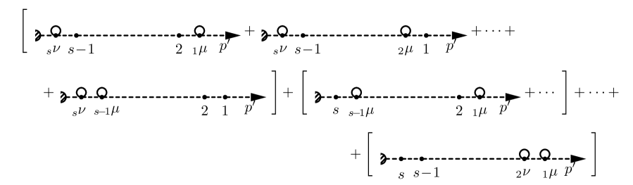
Figure 6: The diagrams with all circled vertices that belong to Set I.

Figure 7: The diagrams with only $\mu$ vertices circled that belong to Set II.

Figure 8: The diagrams with only $q=\nu$ vertices circled that belong to Set III.

Figure 9: The diagrams with ${}_{\nu}\mu$ circled vertices that belong to Set IV. The last term corresponds to the self energy diagram and is to be omitted on the $p$ leg to avoid double counting.

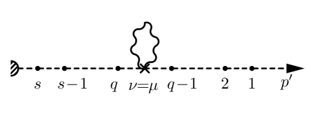
Figure 10: A typical tadpole diagram where the vertices $\mu$, $\nu$ of the $(n+1)^{\rm th}$ $K$ photon have been inserted between the vertices $q$ and $q-1$.

In order to simplify the analysis, we first consider only the $T=0$ contribution which is logarithmically divergent in the IR/soft limit. We will show that various contributions can be combined so that the term-by-term cancellation is more easily seen. This analysis also highlights the role of the tadpole contributions in factorising the IR divergent parts. We will then use the understanding acquired in this analysis to consider the entire finite temperature contribution which contains linear divergences and logarithmic subdivergences that must be factorised as well.

3.1.2.1 $K$ photon insertions with both vertices on the $p^{\prime}$ leg: $T=0$

Tadpole diagrams are proportional to $g_{\mu\nu}$ as per the Feynman rules in Appendix A. (Note the presence of an additional symmetry factor of $1/2$ with respect to the seagull vertex factor shown here.) Hence the $K$ photon insertions of tadpoles on the $p^{\prime}$ leg contribute terms proportional to $k^{2}$ and are IR finite. Thus, it appears at first sight that tadpole diagrams can be neglected when discussing the IR behaviour of scalar QED. However, this is not so, since the contributions from these tadpoles are crucial in obtaining the factorisation and subsequent exponentiation of the IR divergent terms from the $K$ photon insertions. We show this result by first considering the (simpler) $T=0$ case without tadpoles. The contributing diagrams are Sets I to IV, excluding the tadpole contributions in Set IV, which we name as Set IV^′.

In Appendix  C we show that the contributions from various contributing diagrams from Sets I to IV^′ can be expressed as a term proportional to the lower order matrix element, ${\cal{M}}_{n}$, as required, as well as terms linear and quadratic in $k$:

$${\mathcal{M}}_{n+1}^{\mu\nu,p^{\prime}p^{\prime}}(T=0) \propto \left[\left\{(2p^{\prime}+l_{1})_{\mu_{1}}\frac{1}{(p^{\prime}+\mathcal{S}_{1})^{2}}\cdots\frac{1}{(p^{\prime}+\mathcal{S}_{s})^{2}}(V)\cdots\right\}\right]$$ (17)

$$-\left[\left\{(2p^{\prime}+l_{1})_{\mu_{1}}\frac{1}{(p^{\prime}+\mathcal{S}_{1})^{2}}\cdots\frac{1}{(p^{\prime}+\mathcal{S}_{s-1})^{2}}(-2k)_{\mu_{s}}\frac{1}{(p^{\prime}+\mathcal{S}_{s})^{2}}(V)\cdots\right\}\right.+\left\{\cdots\right\}$$

$$+\left\{(2p^{\prime}+l_{1})_{\mu_{1}}\frac{1}{(p^{\prime}+\mathcal{S}_{1})^{2}}\cdots{(2p^{\prime}+2\Sigma_{q-1}+l_{q})_{\mu_{q}}}\frac{1}{(p^{\prime}+\mathcal{S}_{q})^{2}}(-2k)_{\mu_{q}}\cdots(V)\cdots\right\}$$

$$+\left.\left\{\rule{0.0pt}{14.22636pt}\cdots\right\}\right]+\left[\left\{\rule{0.0pt}{14.22636pt}\cdots\right\}\right.+\left\{(2p^{\prime}+l_{1})_{\mu_{1}}\frac{1}{(p^{\prime}+\mathcal{S}_{1})^{2}}\cdots(2p^{\prime}+2\Sigma_{q-1}+l_{q})_{\mu_{q}}\times\right.$$

$$~{}~{}~{}\left\{\frac{1}{(p^{\prime}+\mathcal{S}_{q})^{2}}{(2k\cdot(p^{\prime}+\sum_{q})+k^{2})}\frac{1}{(p^{\prime}+\mathcal{S}_{q})^{2}}\right\}(2p^{\prime}+2{\sum}_{q}+l_{q+1})_{\mu_{q+1}}\cdots$$

$$~{}~{}~{}\left.\frac{1}{(p^{\prime}+\mathcal{S}_{s})^{2}}(V)\cdots\right\}+\left.\left\{\rule{0.0pt}{17.07164pt}\cdots\right\}\right]~{}.$$

Here the zero temperature propagator of a scalar with momentum $p^{\prime}+\sum_{q}$ is $i/((p^{\prime}+\sum_{q})^{2}-m^{2})$, which we have represented as $i/(p^{\prime}+{\cal{S}}_{q})^{2}$. It can be seen that apart from the first term in Eq. 17 which is proportional to the lower order matrix element, ${\cal{M}}_{n}$, the remaining terms are proportional to $(-2k)_{\mu_{q}}$, $2k\cdot P$, and $k^{2}$, with no other $k$ dependence in the denominators. Since $b_{k}$ is even in $k$ (by definition), the terms proportional to either of $(-2k)_{\mu_{q}}$ and $2k\cdot P$ vanish on integration, leaving only the term proportional to ${\cal{M}}_{n}$ and terms proportional to $k^{2}$. Recall that the $T=0$ contribution is logarithmically divergent in the soft photon limit while the finite $T$ contribution has both linear (${\cal{O}}(1)$) and logarithmic (${\cal{O}}(k)$) divergences; consequently, terms proportional to $k^{2}$ are IR finite. While these ${\cal{O}}(k^{2})$ terms do not spoil the IR finiteness of the theory, they also do not allow the $(n+1)^{\rm th}$ matrix element to be expressed as purely proportional to the lower $n^{\rm th}$ order matrix element, which would have enabled the IR divergent pieces to be factorised and exponentiated to all orders, eventually cancelling with the corresponding IR divergent parts from the real photon contributions.

A straightforward calculation of the contribution of the hitherto neglected tadpole diagrams in Set IV (see Appendix C shows that this contribution exactly cancels these ${\cal{O}}(k^{2})$ terms left over in Eq. 17 above; hence the total contribution from inserting a vritual $K$ photon in all possible ways such that both vertices are on the $p^{\prime}$ leg is simply a term proportional to the lower order matrix element, as required. With the understanding that the tadpole contributions are crucial in achieving this result, we now go on to consider the finite temperature case of interest.

3.1.2.2 $K$ photon insertions with both vertices on the $p^{\prime}$ leg: finite $T$

We use the insight we have gained from the zero temperature case to complete the calculation for the general thermal case when both the $K$ photon vertices are inserted into the same leg. The same diagrams contribute; we consider each set in turn and make use of the generalised thermal identities discussed in Appendix B since the propagators are no longer simple and have a $2\times 2$ matrix form. Generalised identities are used to get term by term cancellations; as in the zero temperature case, there are many left-over terms due to the presence of the additional 4-point vertices, in contrast to the fermionic case. This is the most complex of the calculations, and most of the details are relegated to Appendix C. The grouping of terms in order to cancel them is made easier by the understanding gained from considering the zero temperature case.

As in the zero temperature case, there are many terms contributing to the various Sets. It is shown in Appendix C that left-over terms of Sets $(I+II+III)$ cancel against corresponding terms in Set IV, leaving behind a term proportional to the lower order matrix element ${\cal M}_{n}$, as required, and towers of terms linear in $k$. The cancellation occurs as follows. The contribution from Set IV can be expressed as,

$${\cal{M}}_{n+1}^{\mu\nu,p^{\prime}p^{\prime},IV} \propto\left\{\left[A_{s}-B_{s}+C_{s}\right]\right\}+\left\{\cdots\right\}+\left\{\left[A_{1}-B_{1}+C_{1}\right]\right\}+\left\{\left[-B_{0}+C_{0}\right]\right\}~{},$$ (18)

where

$$A_{q} =(2p^{\prime}+l_{1})_{\mu_{1}}S^{12}_{p^{\prime}+\sum_{1}}(2p^{\prime}+2\Sigma_{1}+l_{2})_{\mu_{2}}\cdots\left[S^{q-1,q}_{p^{\prime}+\sum_{q-1}+k}\delta_{t_{\mu},t_{q-1}}\delta_{t_{\nu},t_{q}}\right]\cdots(\hbox{no }k)~{},$$

$$B_{q} =(2p^{\prime}+l_{1})_{\mu_{1}}S^{12}_{p^{\prime}+\sum_{1}}(2p^{\prime}+2\Sigma_{1}+l_{2})_{\mu_{2}}\cdots\left[S^{q-1,q}_{p^{\prime}+\sum_{q-1}}\delta_{t_{\mu},t_{q-1}}\delta_{t_{\nu},t_{q-1}}\right]\cdots(\hbox{no }k)~{},$$

$$C_{q} =(2p^{\prime}+l_{1})_{\mu_{1}}S^{12}_{p^{\prime}+\sum_{1}}(2p^{\prime}+2\Sigma_{1}+l_{2})_{\mu_{2}}\cdots\left[S^{\nu,q}_{p^{\prime}+\sum_{q}}(2p^{\prime}+2\Sigma_{q-1})\cdot k\,\delta_{t_{\mu},t_{\nu}}S^{\nu,q}_{p^{\prime}+\sum_{q}}\right]\cdots(\hbox{no }k)~{},$$ (19)

where “no $k$” indicates that the remaining terms do not have any $k$ dependence. Here the term $(-B_{0}+C_{0})$ arises from self-energy corrections on the $p^{\prime}$ leg, with $B_{i}$ proportional to ${\cal M}_{n}$. Note that all $C_{i}$ are odd in $k$.

Details of the calculation for Sets I, II, and III are given in Appendix C. Combining Sets I, II and III, we have,

$${\cal{M}}_{n+1}^{\mu\nu,p^{\prime}p^{\prime},I+II+III} =\left[\sum_{q=1}^{s}B_{q}-\sum_{q=0}^{s}A_{q}+Y\right]$$ (20)

where $Y$ is defined in Eq. C.47 in Appendix C and each term in $Y$ is proportional to $(-2k)_{\mu_{q}}$. Hence both the contributions of $C_{q}$ and $Y$ have linear powers of $k$ in the numerator, and no other dependence on $k$ apart from the overall factors such as $b_{k}$, etc. Hence these terms are odd in $k\leftrightarrow-k$ and vanish. We see that the $A_{q}$ terms cancel between the contributions of Set IV in Eq. C.46 and Sets ($I+II+III)$ in Eq. C.47, as also all the $B_{q}$ except for $-B_{0}$ which remains as the only left over piece when all sets are combined and we further recall that this term is proportional to the lower order matrix element, as in the $T=0$ case.

Note that the ${\cal O}(k^{2})$ terms terms are present in the two contributing graphs corresponding to each term in the typical circled vertices of Set IV and exactly cancel against one another. While the ${\cal O}(k^{2})$ terms, and hence, the tadpole contributions are IR finite and do not pose any problems for the theory, it is not just simply a preference that these be included with the IR finite $G$ photon contributions; $b_{k}$ was designed to isolate the IR singular terms and resum them; hence the presence of such ${\cal O}(k^{2})$ terms in addition to the term proportional to the lower order matrix element, precludes the factorisation and resummation of the $K$ photon contributions to all orders; hence it is a matter of satisfaction that such ${\cal O}(k^{2})$ terms cancel exactly.

The sum of the contributions from all four sets of diagrams with all possible insertions of the $(n+1)^{\rm th}$ $K$ photon, with both vertices on the $p^{\prime}$ leg, is therefore a term that contains the IR divergence and is proportional to the lower order matrix element with no additional finite contributions, as is the case with the zero temperature theory and fermionic QED. Putting back the overall factors, we have,

$${\cal M}^{p^{\prime}p^{\prime},K\gamma}_{n+1}=+ie^{2}\int\frac{{\rm d}^{4}k}{(2\pi)^{4}}\,\delta_{t_{\mu},t_{1}}\,\delta_{t_{\nu},t_{1}}\,b_{k}(p^{\prime},p^{\prime})\,D^{t_{\mu},t_{\nu}}(k)~{}{\cal M}_{n}~{}.$$ (21)

Since $t_{1}=1$ necessarily, it depends only on the $D^{11}$ photon propagator, as before.

3.1.3 Both $K$ photon insertions on the $p$ leg alone

A similar analysis can be done for the case when both the vertices of the inserted $(n+1)^{\rm th}$ $K$ photon are on the $p$ leg. As discussed in GY, the outermost self energy insertion graph is neglected here to compensate for wave function renormalisation, due to which the sum of contributions for all possible insertions on the $p$ leg adds up to zero. As shown in Appendix C, the term $(-B_{0}+C_{0})$ arises from self-energy corrections on the $p^{\prime}$ leg. A similar contribution occurs when the virtual $K$ photon is inserted on the $p$ leg. Hence when we remove the self-energy correction on the $p$ leg to account for wave function renormalisation, we remove the term corresponding to $(-B_{0}+C_{0})$. (The contribution of $C_{0}$ is in any case zero since it is odd in $k$.) The total contribution for the insertion of a virtual $K$ photon in all possible ways on the $p^{\prime}$ leg added up to $-B_{0}$. When this is removed to account for wave function renormalisation for insertions on the $p$ leg, we find that the total contribution vanishes.

Since this compensation could have been included in either of the legs, we symmetrise over the two possibilities, thus giving us the contributions:

$${\cal M}^{p^{\prime}p^{\prime},K\gamma}_{n+1} =+ie^{2}\frac{1}{2}\,\int\frac{{\rm d}^{4}k}{(2\pi)^{4}}\,\delta_{t_{\mu},t_{1}}\,\delta_{t_{\nu},t_{1}}\,b_{k}(p^{\prime},p^{\prime})\,D^{t_{\mu},t_{\nu}}(k)~{}{\cal M}_{n}~{},$$

$${\cal M}^{pp,K\gamma}_{n+1} =+ie^{2}\frac{1}{2}\,\int\frac{{\rm d}^{4}k}{(2\pi)^{4}}\,\delta_{t_{\mu},t_{1}}\,\delta_{t_{\nu},t_{1}}\,b_{k}(p,p)\,D^{t_{\mu},t_{\nu}}(k)~{}{\cal M}_{n}~{}.$$ (22)

The contribution is once more proportional to the lower order matrix element and depends on the $D^{11}$ part of the inserted photon propagator alone.

3.1.4 Inclusion of ‘disallowed diagrams’

Certain ‘disallowed diagrams’ may contribute at higher orders. For instance, the outermost self-energy insertion graph is removed at a certain order to account for wave function renormalisation. However, while making $K$ or $G$ photon insertions at the next higher order, these lower order diagrams must be included, as these can give rise to allowed graphs at the next order. As in the case of the zero temperature theories, these terms add to zero. There is an additional disallowed diagram in the thermal case that must be similarly included: these are lower order graphs with ‘outermost’ vertices next to the $p^{\prime}$ or $p$ external legs that are of thermal unphysical type with $t_{1}=2$. A calculation shows that these diagrams also do not contribute at the next higher order.

3.1.5 The total $K$ photon contribution

The total contribution from the insertion of the $(n+1)^{\rm th}$ virtual $K$ photon therefore is,

$${\cal{M}}_{n+1}^{K\gamma,{\rm tot}}= \frac{ie^{2}}{2}\int\frac{{\rm d}^{4}k}{(2\pi)^{4}}\,\left\{\delta_{t_{\mu},t_{1}}\,\delta_{t_{\nu},t_{1}}\,D^{t_{\mu},t_{\nu}}(k)\,\left[b_{k}(p^{\prime},p^{\prime})+b_{k}(p,p)\right]\right.$$

$$+\left.\delta_{t_{\mu},t_{V}}\,\delta_{t_{\nu},t_{V}}\,D^{t_{\mu},t_{\nu}}(k)\,\left[-2b_{k}(p^{\prime},p)\right]\right\}{\cal{M}}_{n}~{},$$

$$\equiv\left[B\right]{\cal{M}}_{n}~{},$$ (23)

where

$$B =\frac{ie^{2}}{2}\int\frac{{\rm d}^{4}k}{(2\pi)^{4}}\,D^{11}(k)\,\left[b_{k}(p^{\prime},p^{\prime})-2b_{k}(p^{\prime},p)+b_{k}(p,p)\right]~{},$$

$$\equiv\frac{ie^{2}}{2}\int\frac{{\rm d}^{4}k}{(2\pi)^{4}}\,D^{11}(k)\,\left[J^{2}(k)\right]~{}.$$ (24)

In Eq. 24 we have used the fact that the thermal types of the hard/external vertices must be type-1; $t_{1}=t_{V}=1$, so that each term is proportional to the (11) component of the photon contribution. This will be crucial to achieve the cancellation between virtual and real photon insertions, as we show below.

Hence the structure of the contribution from virtual $K$ photon insertion is the same as in the $T=0$ case; however, note that, due to the thermal contributions in the photon propagator, there are both linear and logarithmic divergences in these terms. Demonstration of the cancellation of the linear divergences follows the same route as that of GY at $T=0$; the demonstration of cancellation of the logarithmic subdivergences is discussed separately later.

3.2 Insertion of virtual $G$ photons

In GY, it was shown that insertion of a virtual $G$ photon into the $n$ vertex graph with only 3-point vertices gives finite contributions. The key point was that the $G$ photon contribution at $T=0$ was proportional to

$${\cal{M}}_{n+1}^{G\gamma;T=0} \propto\left\{g_{\mu\nu}-b_{k}(p_{f},p_{i})k_{\mu}k_{\nu}\right\}\times p_{f}^{\mu}\,p_{i}^{\nu}~{},$$

$$=0+{\cal{O}}(k)~{}.$$ (25)

Since the leading divergence for the $T=0$ theory is a logarithmic one, terms proportional to powers of $k$ in the numerator are IR finite; hence the $G$ photon contribution was IR finite.

At finite temperatures, there are two major modifications: one due to the thermal part of the photon propagator and the other due to the thermal part of the scalar propagator. We start by considering the contribution due to the thermal part of the photon propagator. Although there are different types of thermal fields and hence four different photon propagators, ${\cal D}^{ab}_{\mu\nu}$, all of them have the same leading IR behaviour: the divergence is a linear one due to the presence of the term in the photon propagator that is proportional to

$$2\pi\delta(k^{2})N(|k^{0}|)\equiv 2\pi\delta(k^{2})\frac{1}{\exp^{|k^{0}|/T}-1}~{}.$$ (26)

This is cancelled for the $G$ photons in exactly the same way as the $T=0$ case. However, there is also a logarithmic subdivergence arising from terms linear in $k$ in the numerator whereas these terms are IR finite in the $T=0$ case. Proving the IR finiteness of these contributions is the central result of this paper. A detailed case-by-case analysis can be found in Appendix D.

We start by ignoring the $T=0$ parts of the propagators and concentrate on the thermal parts alone. Since the thermal part of the photon propagator includes an overall $\delta(k^{2})$, there are two simplifications that result. First, the coefficient factor $b_{k}(p_{f},p_{i})$ simplifies to

$$b^{T\neq 0}_{k}(p_{f},p_{i})=\frac{p_{f}\cdot p_{i}}{p_{f}\cdot k\;\;p_{i}\cdot k}~{}.$$ (27)

In addition, we can ignore $k^{2}$ terms in the scalar propagators. The complete structure of this matrix element can be written as,

$${\cal M}^{G\gamma}_{n+1} \sim\int d^{4}k\left[\frac{i}{k^{2}+i\epsilon}\delta_{t_{\mu},t_{\nu}}\pm 2\pi\delta(k^{2})N(|k|)D^{t_{\mu},t_{\nu}}_{T}\right]\,\left[g^{\mu\nu}-b_{k}k^{\mu}k^{\nu}\right]\,\left[{\rm scalar}\right]_{\mu\nu},$$ (28)

where the terms in the first two square brackets correspond to terms in the definition of the $G$ photon propagator, with the relative sign in the first being determined by the thermal field indices, $t_{\mu},t_{\nu}$. The last term represents the contribution from the $\mu$ and $\nu$ virtual $G$ photon insertions on the scalar legs, $p$ and $p^{\prime}$, and are products of the vertex and propagator factors. Combining the second term in Eq. 28 with the vertex factors at only the $\mu$ and $\nu$ vertices (assuming them to be 3-point for now) in the third term, we get,

$$\begin{multlined}\left[g^{\mu\nu}-b_{k}k^{\mu}k^{\nu}\right]\,\left\{S^{q-1,\mu}_{p_{f}+\sum_{q-1}}\left[(2p_{f}+2\Sigma_{q-1}+k)_{\mu}\,S^{\mu,q}_{p_{f}+\sum_{q-1}+k}(2p_{f}+2\Sigma_{q-1}+2k+l_{q})_{\mu_{q}}\right]\right\}\times\\ \left\{S^{m+1,\nu}_{p_{i}+\sum_{m}+k}\left[(2p_{i}+2\Sigma_{m}+k)_{\nu}\,S^{\nu,m}_{p_{f}+\sum_{m}}(2p_{i}+2\Sigma_{m-1}+l_{m})_{\mu_{m}}\right]\right\}\,\end{multlined}\left[g^{\mu\nu}-b_{k}k^{\mu}k^{\nu}\right]\,\left\{S^{q-1,\mu}_{p_{f}+\sum_{q-1}}\left[(2p_{f}+2\Sigma_{q-1}+k)_{\mu}\,S^{\mu,q}_{p_{f}+\sum_{q-1}+k}(2p_{f}+2\Sigma_{q-1}+2k+l_{q})_{\mu_{q}}\right]\right\}\times\\ \left\{S^{m+1,\nu}_{p_{i}+\sum_{m}+k}\left[(2p_{i}+2\Sigma_{m}+k)_{\nu}\,S^{\nu,m}_{p_{f}+\sum_{m}}(2p_{i}+2\Sigma_{m-1}+l_{m})_{\mu_{m}}\right]\right\}\,$$ (31)

$$=\left[4P_{f}\cdot P_{i}+2(P_{f}+P_{i})\cdot k-4b_{k}P_{f}\cdot k\,P_{i}\cdot k\right]\left[S^{q-1,\mu}S^{\mu,q}S^{m+1,\nu}S^{\nu,m}(\cdots)_{\mu_{q}}(\cdots)_{\mu_{m}}\right]~{},$$

$$=\left[0(p_{f}\cdot p_{i})+2(p_{f}+2p_{i})\cdot k\right]\cdots~{},$$ (32)

where we have used $P_{f}=p_{f}+\sum_{i=1}^{q-1}l_{i}$ and $P_{i}=p_{i}+\sum_{i=1}^{m-1}l_{i}$. In the soft limit, replacing $P_{f}\to p_{f}$, $P_{i}\to p_{i}$, and substituting for $b_{k}$ from Eq. 27, we get the last line of Eq. 32. We see that the leading $(p_{f}\cdot p_{i})$ term vanishes (indeed, $b_{k}$ was chosen for this very reason) and the term in the square brackets is exact with no further corrections. The ellipses refer to the contribution from the remaining vertices and propagators, some of which (the set of vertices and propagators that lie between the $\mu$ and $\nu$ vertices) also depend on $k$. Substituting this back in Eq. 28, we have,

$${\cal M}^{G\gamma}_{n+1}\sim \int d^{4}k\left[\frac{i}{k^{2}+i\epsilon}\delta_{t_{\mu},t_{\nu}}\pm 2\pi\delta(k^{2})N(|k|)D_{t_{\mu},t_{\nu}}\right]\left[0(p_{f}\cdot p_{i})+2(p_{f}+2p_{i})\cdot k\right]\left[{\rm scalar}\right]_{\not{\mu}\not{\nu}}~{},$$ (33)

where the slashes on $\mu$ and $\nu$ indicate that the contribution from these vertices have been removed and simplified as per Eq. 32 and,

$$\left[{\rm scalar}\right]_{\not{\mu}\not{\nu}} \sim\left[{\cal O}(1)+{\cal O}(k)+{\cal O}(k^{2})+\cdots\right]~{},$$ (34)

where we have indicated the powers of $k$ in the numerator of the matrix element from the scalar contribution above.

We know that the $T=0$ part is logarithmically divergent while the leading thermal divergence is linear. The factor $b_{k}$ is so chosen so that the $(p_{f}\cdot p_{i})\times[{\cal O}(1)]$ term, obtained by combining Eqs. 33 and 34, vanishes. Note that this term gives rise to the leading log divergence at $T=0$ (from the $1/(k^{2}+i\epsilon)$ term in the photon propagator) as well as the leading linear divergence at $T\neq 0$ (from the $\delta(k^{2})N(|k|)$ term). The remaining $T=0$ part is IR finite since any power of $k$ in the numerator renders the term finite.

At $T\neq 0$, in addition, the logarithmic subdivergence arising from the $(p_{f}\cdot p_{i})\times[{\cal O}(k)]$ term from Eqs. 33 and 34, also vanishes since the coefficient of this term is zero. But there is a term arising from the $((p_{f}+p_{i})\cdot k)\times[{\cal O}(1)]$ factor in the thermal part, that appears to be a logarithmic subdivergence. We however observe that the $[{\cal O}(1)]$ terms in the scalar part are symmetric under the interchange $(k\leftrightarrow-k)$; since the term $((p_{f}+p_{i})\cdot k)$ is linear in $k$, the entire contribution is odd under this interchange, so that this potential subdivergent log contribution vanishes. Higher order terms arising from even powers of $k$ in the integrand are IR finite. Hence the $G$ photon insertions are IR finite.

We have implicitly assumed that there are no divergences associated with the photon momenta $l_{i}$ in the lower order graphs (that is, from ${\cal M}_{n}$). This is not necessarily true; divergences can potentially arise from any of the soft photons in the graph. Here, the procedure, as shown by GY, is to separate out the photon momenta into groups that cause an IR divergence and those that do not. It is then possible to ignore the latter group and construct so-called “skeletal graphs” where the divergence arises only when each of the controlling momenta, $l_{i},i=1,\cdots,m$, simultaneously vanish. It was shown in Refs. [4, 12] that $G$ photon insertions are finite with respect to all such controlling momenta for a theory of charged fermions at zero and finite temperature. In Appendix D we show that this holds for scalars at finite temperature as well.

This result also holds when we extend the analysis to include the possibility that the $\mu$ and $\nu$ vertex insertions are of 4-point type, or even that some or all of the vertices in the lower order graph are of 4-point type as well; each of these cases is dealt with in detail in Appendix D. The final generalisation is when we include thermal effects in the scalar propagator as well (those in the vertices are quite trivial to deal with). We discuss this below.

3.2.1 Effect of including thermal scalars

When the scalar field is also thermal, it is not sufficient to consider the $1/(P^{2}-m^{2})$ part of the scalar propagator. There are factors of the scalar number operator, $N_{S}$, that can cause a potential divergence since the scalar fields are bosons with,

$$N_{S}(|P^{0}|)=\frac{1}{\exp[|P^{0}|/T]-1}\;\stackrel{{\scriptstyle P^{0}\to 0}}{{\longrightarrow}}\;\frac{1}{|P^{0}|}~{},$$ (35)

in contrast to the fermionic case where the number operator is finite, $N_{f}\to 1/2$, as $|P^{0}|\to 0$; so we need to check that this result holds when the scalars are thermal as well. We begin as usual by considering graphs with only 3-point vertices.

The numerator factors arising from the scalar-photon vertices acquire only irrelevant modifications when temperature effects are included; hence the structure of the vertices, that were crucial in obtaining the cancellation of the leading divergence of the $G$ photon contributions between the $g_{\mu\nu}$ and $b_{k}k_{\mu}k_{\nu}$ terms in Eq. 32, still holds. We need to consider only the terms linear in $k$ that can give rise to subleading logarithmic divergences as discussed above.

We, therefore, examine the finite temperature dependence of the scalar propagators. In contrast to the case of thermal photons, the momentum $p_{f}$ (or $p_{i}$) flows through all the scalar lines and this controls the behaviour in the soft limit. The pure $L_{0}(l_{i})\sim 1/(l_{i}^{2}-m^{2})$ dependence at $T=0$ is replaced by a sum of $L_{0}(l_{i})$ and $L_{T}(l_{i})\sim\delta(l_{i}^{2}-m^{2})$ terms. Hence, none, some, or all the scalar propagators can have thermal contributions. The case where all scalar propagators correspond to $L_{0}$ is the case that we have studied so far.

While the two propagators have the same dimensional dependence on $k$, $L_{T}(l_{i}=P+k)$ contains a delta-function $\delta((P+k)^{2}-m^{2})$ dependence which either makes the term finite or else leads to a constraint where $k^{0}$ is related to combinations of the remaining (controlling) momenta and hence there is no (logarithmic sub)divergence associated with this term. This holds even when more than one of the scalar propagators is a thermal $L_{T}$ type. The detailed analysis for adding a $G$ photon to a lower order graph with thermal electrons, and having one or more momenta in the controlling set, can be found in Ref. [12] and applies to the case of charged scalars as well. Hence the $G$ photon insertion is IR finite when we consider the entire thermal structure of the theory, both for charged scalars and photons, and even if the charged particles are fermions. More details are found in Appendix D. Finally, the cases when some of the vertices are $K$ photons or real photon vertices is also discussed in Appendix D.

As before, we have to verify that when we “flesh out” skeletal graphs and include self-energy or other terms, the graph remains IR finite; this is also shown in Appendix D. This concludes the proof that the entire virtual $G$ photon insertions of the full finite temperature theory (with both charged fermions and scalars) are in general IR finite.

3.3 The final matrix element for virtual photons

We have obtained the familiar result that the (IR divergent) contribution of the $K$ photon insertions is proportional to the lower order matrix element, ${\cal M}_{n}$ while the $G$ photon insertions are finite. We proceed as in the case of $T=0$ scalar QED or thermal fermionic QED and consider the contribution of the $n^{\rm th}$ order graph with $n_{K}$ virtual $K$ photons and $n_{G}$ virtual $G$ photons. Hence $n=n_{K}+n_{G}$ and there are at most $n$ vertices (since some can be seagulls or tadpoles). As a consequence of the Bose symmetry for the $n$ photons, each distinct graph can arise in $n!/n_{K}!\,n_{G}!$ ways, so that the total matrix element can be expressed as a sum of all possible individual contributions,

$$\frac{1}{n!}\,{\cal M}_{n}=\sum_{n_{K}=0}^{n}\frac{1}{n_{K}!}\frac{1}{n-n_{K}!}{\cal M}_{{n_{G}},{n_{K}}}~{}.$$ (36)

Summing over all orders, we get

$$\sum_{n=0}^{\infty}\frac{1}{n!}{\cal M}_{n} =\sum_{n=0}^{\infty}\sum_{n_{K}=0}^{n}\frac{1}{n_{K}!}\frac{1}{n-n_{K}!}{\cal M}_{{n_{G}},{n_{K}}}~{},$$

$$=\sum_{n_{K}=0}^{\infty}\sum_{n_{G}=0}^{\infty}\frac{1}{n_{K}!}\frac{1}{n_{G}!}{\cal M}_{{n_{G}},{n_{K}}}~{},$$ (37)

and we use the result that the $K$ photon contribution is proportional to the lower order matrix element to obtain:

$${\cal M}_{{n_{G}},{n_{K}}} =(B)^{n_{K}}M_{n_{G},0}\equiv(B)^{n_{K}}M_{n_{G}}~{},$$ (38)

where $B$ as defined in Eq. 24 is the contribution from each $K$-photon insertion and can be isolated and factored out, leaving only the IR finite $G$-photon contribution, ${\cal M}_{n_{G}}$. Re-sorting and collecting terms, we obtain the requisite exponential IR divergent factor:

$$\sum_{n=0}^{\infty}\frac{1}{n!}{\cal M}_{n} =\sum_{n_{K}=0}^{\infty}\frac{(B)^{n_{K}}}{n_{K}!}\sum_{n_{G}=0}^{\infty}\frac{1}{n_{G}!}{\cal M}_{n_{G}}~{},$$

$$={\rm e}^{B}\sum_{n_{G}=0}^{\infty}\frac{1}{n_{G}!}{\cal M}_{n_{G}}~{}.$$ (39)

Again we highlight that this factorisation was made possible since the $K$-photon insertions gave precisely one term and no additional pieces, IR-finite or otherwise; this occurred due to the presence of both 3-point and 4-point vertices in the theory. The resulting cross section including only the virtual photon contributions to all orders is,

$$\sigma^{\rm virtual} \propto\int{\rm d}\phi_{p^{\prime}}(2\pi)^{4}\delta^{4}(p+q-p^{\prime})\left|\sum_{n=0}^{\infty}\frac{1}{n!}{\cal M}_{n}\right|^{2}~{},$$

$$=\int{\rm d}\phi_{p^{\prime}}(2\pi)^{4}\delta^{4}(p+q-p^{\prime})~{}|Z|^{2}~{}\sigma^{\rm virtual}_{G}~{},$$ (40)

where ${\rm d}\phi_{p^{\prime}}$ is the phase space factor corresponding to the final state scalar with momentum $p^{\prime}$ and a(n irrelevant) flux factor in the denominator has been suppressed. The IR-finite part is contained in the last term and the IR divergent part is contained in the exponent,

$$|Z|^{2} \equiv\exp\left(B+B^{*}\right)~{},$$ (41)

and will be shown below to cancel against a corresponding contribution from real (soft) photon emission/absorption with respect to the heat bath, thus indicating that thermal scalar electrodynamics is also IR finite at all orders.

3.4 Emission/absorption of real photons

There is a major difference in the thermal case: real photons can be emitted into or absorbed from the heat bath. Again, the real photon vertex can be either on the $p$ or $p^{\prime}$ leg, and the contributions of the two can be independently calculated. The insertion can be a 3-point vertex (photon inserted on the $p$ or $p^{\prime}$ leg at a new vertex $\mu$) or a 4-point vertex (photon inserted on an already existing vertex, giving seagull but not tadpole diagrams since a real photon is actually emitted/absorbed).

Unlike the virtual photon insertions, physical momentum is carried away or brought in by the real photon. Without loss of generality, this can be accounted for by retaining the momenta of the external scalar legs to be $p$ and $p^{\prime}$ and adjusting the momentum at the special vertex $V$ to maintain energy-momentum conservation. Hence the factors are somewhat different from the virtual photon case: when the $(n+1)^{\rm th}$ photon is emitted from the $p$ leg, the momentum of the scalar/fermion to the right of the insertion $\mu$ is $(p+\sum_{i=1}^{q}l_{i}-k)$ where $q$ is the vertex immediately to the left of $\mu$; here $l_{i}$ are the photon momenta emitted/absorbed at the $i^{\rm th}$ vertex. Similarly, for an emission from the $p^{\prime}$ leg, the momentum of the scalar/fermion to the left of $\mu$ is $(p^{\prime}+\sum_{i=1}^{q}l_{i}+k)$, where $q$ is the vertex immediately to the right of $\mu$. If the photon is absorbed rather than emitted, the sign of $k$ is reversed.

Since the real photon insertions contribute to $|{\cal{M}}|^{2}$, that is, to the cross section, we need to consider thermal modifications to the phase space. The thermal phase space element corresponding to the $i^{\rm th}$ real photon with momentum $k_{i}$ is given by,

$${\rm d}\phi_{i} =\frac{{\rm d}^{4}k_{i}}{(2\pi)^{4}}\,2\pi\delta(k_{i}^{2})\,\left[\theta(k_{i}^{0})+N(|\boldsymbol{k_{i}}|)\right]~{}.$$ (42)

Here emission of photons corresponds to $k_{i}^{0}>0$ and absorption to $k_{i}^{0}<0$, thus giving the correct statistical factors of $N\!+\!1$ for photon emission into, and $N$ for photon absorption from, the heat bath at temperature $T$. Again, the presence of the thermal number operator worsens the divergence in the case of real photon emission/absorption as well, giving a leading IR dependence that is linear, since $N\sim 1/k$ in the soft limit. Note that the presence of the same term acts as an UV cut off when $k\to\infty$.

We proceed as in GY, re-writing the polarisation sum in the cross section and separating it into a $\widetilde{K}$ part that potentially contains the entire IR divergent part and an IR finite $\widetilde{G}$ photon part:

$$\sum_{\rm pol}\epsilon^{*}_{\mu}(k)\,\epsilon_{\nu}(k)=-g_{\mu\nu}~{},$$ (43)

with

$$g_{\mu\nu} =\left\{\left[g_{\mu\nu}-\tilde{b}_{k}(p_{f},p_{i})k_{\mu}k_{\nu}\right]+\left[\tilde{b}_{k}(p_{f},p_{i})k_{\mu}k_{\nu}\right]\right\}~{},$$

$$\equiv\left\{\left[\widetilde{G}_{\mu\nu}\right]+\left[\widetilde{K}_{\mu\nu}\right]\right\}~{},$$ (44)

where the tildes have been used to distinguish the real from the virtual photon contributions. Since $k^{2}=0$ for both real photon emission and absorption, we define,

$$\tilde{b}_{k}(p_{f},p_{i})=b_{k}(p_{f},p_{i})\Big{|}_{k^{2}=0}=\frac{p_{f}\cdot p_{i}}{k\cdot p_{f}\;k\cdot p_{i}}~{},$$ (45)

where $p_{i}$ ($p_{f}$) corresponds to the initial (final) momentum of the hard scalar in ${\cal{M}}$ ($\cal{M}^{*}$) where the real photon of momentum $k$ is inserted.

3.4.1 Emission/absorption of real $\widetilde{K}$ photons

The proof that the contribution from $\widetilde{K}$ photons is IR divergent and can be factored is much simpler than the corresponding case of virtual photons. The key point to note is that real photons, whether emitted or absorbed, correspond to thermal type 1 photons, so that the inserted vertex (either $\mu$ or $\nu$) is of type 1 alone. This is critical in obtaining a cancellation against the virtual photon contribution and the significance of this virtual contribution being proportional to $D^{11}$ alone, as shown in Eqs. 16 and 22, is now clear.

The calculation for photon emission proceeds exactly as in the case of virtual photon vertex insertion on a $p$ or $p^{\prime}$ leg (see diagrams shown in Fig. 5). Again, there is a term-by-term cancellation, leading to a factor proportional to the matrix element of the $n$ photon diagram, ${\cal{M}}_{n}$. Similar insertions on the $p$ leg give a result proportional to $-{\cal{M}}_{n}$; the difference in sign with the case of insertion of $b_{k}(p^{\prime},p)$ virtual $K$ photons is due to the fact that the real photon momentum is always out-going for emitted photons; while the virtual momentum enters/leaves at the $\nu/\mu$ vertex. The overall sign is reversed in the case of photon absorption; however, this is irrelevant and unobserved in the cross section. Adding the two terms and squaring gives the contribution of the real $\widetilde{K}$ photon insertion to be an overall factor multiplying the $n^{\rm th}$ order cross section, proportional to,

$$\left|{\cal{M}}_{n+1}^{\widetilde{K}\gamma,{\rm tot}}\right|^{2} \propto-e^{2}\left[\tilde{b}_{k}(p,p)-2\tilde{b}_{k}(p^{\prime},p)+\tilde{b}_{k}(p^{\prime},p^{\prime})\right]~{},$$

$$\equiv-e^{2}\widetilde{J}^{2}(k)~{}.$$ (46)

The result holds even when some vertices of the lower order graph are 4-point ones, or correspond to virtual photon insertions as well; this follows from the arguments given for the virtual $K$ photon insertions in Appendix C.

Before discussing the cross section, we will first complete the discussion on insertions of real $\widetilde{G}$ photons, which, as expected, will be IR finite.

3.4.2 Emission/absorption of real $\widetilde{G}$ photons

The proof of IR finiteness of the real $\widetilde{G}$ photon cross section follows from the same argument as for the virtual $G$-photon insertion and is not repeated here in detail. Specifically, the case where the insertions are on different legs ($p^{\prime}$ and $p$) is relevant for the real photon insertions. All the cases such as including both 3- and 4-point vertices, including thermal effects in both photon and scalar propagators, etc., hold here; there are no tadpole diagrams in this case and also no quadratic ${\cal O}(k^{2})$ contribution that needs to be cancelled.

The key point to note here is the $k$-dependence of the thermal part. The leading divergence (logarithmic in the zero temperature case and linear in the finite temperature case) cancels as before, between the $g_{\mu\nu}$ and the $\tilde{b}_{k}k_{\mu}k_{\nu}$ parts of $\widetilde{G}$, owing to the definition of $\tilde{b}_{k}$. We are thus concerned only with terms with powers of $k$ in the numerator which potentially give logarithmic subdivergences.

The main difference between virtual and real photon insertion is that the phase space factor is not symmetric under $k\leftrightarrow-k$ because of the presence of the theta function, as seen from Eq. 42. However, the finite temperature part of the phase space is symmetric under this exchange since it includes both photon emission and absorption. These are anyway the only contributions of interest since any powers of $k$ in the numerator are finite with respect to the $T=0$ part. This symmetry enables us to symmetrise the integrand with respect to $k\leftrightarrow-k$ and obtain the analogous result that real $\widetilde{G}$ photon insertions are IR finite. Notice that application of the symmetry requires the presence of both soft photon emission and absorption terms.

Again, the result holds when one of the photons with momentum $k_{l}$ contributes through its $T=0$ part; in this case, its corresponding momentum cannot be flipped since its phase space is not symmetric under this exchange. We apply the same logic as with skeletal graphs in the virtual photon case: if this photon is not a part of the controlling set, there is no divergence associated when it vanishes and this gives us no trouble. If it is a part of the controlling set, then the sub-divergence occurs only when all (including this) momenta vanish simultaneously; however, any power of $k_{l}$ in the numerator renders the contribution finite since it contributes through its $T=0$ part and so again its contribution is finite. The analysis holds when arbitrary number of these photons contribute through their $T=0$ parts; also when some of these are virtual photons, since their contribution is always symmetric in the loop momentum.

Hence, $\widetilde{G}$ photon emissions give a finite contribution to the cross section.

3.4.3 The total cross section from real photon emission/absorption

Consider an $n^{\rm th}$ order graph with an arbitrary number of $\widetilde{K}$ and $\widetilde{G}$ photon insertions. Now $n_{K}$ $\widetilde{K}$ and $n_{G}$ $\widetilde{G}$ real photon emission/absorption can occur in $n!/n_{K}!n_{G}!$ ways; $n=n_{K}+n_{G}$, and each real photon carries away/brings in a physical momentum $k_{l}$ from/to the process. Dividing by $n!$ due to $n$ identical photons in the final state, to this order, we have,

$${\rm d}\sigma^{\rm real}_{n} =\begin{multlined}\sum_{n_{K}=0}^{n}\int\frac{1}{n_{K}!}\left[\prod_{i=1}^{n_{K}}{\rm d}\phi_{i}\left\{-e^{2}\widetilde{J}^{2}(k_{i})\right\}\right]\times\frac{1}{n_{G}!}\left[\prod_{j=n_{K}+1}^{n}{\rm d}\phi_{j}\left\{-\widetilde{G}_{\mu\nu}\left|{\cal M}^{\mu\nu,\tilde{G}\gamma,tot}_{n_{G}}\right|^{2}\right\}\right]\times\\ \quad\quad(2\pi)^{4}\delta^{4}\left(p+q-p^{\prime}-\sum_{l=1}^{n}(-1)^{l}k_{l}\right)~{},\end{multlined}\sum_{n_{K}=0}^{n}\int\frac{1}{n_{K}!}\left[\prod_{i=1}^{n_{K}}{\rm d}\phi_{i}\left\{-e^{2}\widetilde{J}^{2}(k_{i})\right\}\right]\times\frac{1}{n_{G}!}\left[\prod_{j=n_{K}+1}^{n}{\rm d}\phi_{j}\left\{-\widetilde{G}_{\mu\nu}\left|{\cal M}^{\mu\nu,\tilde{G}\gamma,tot}_{n_{G}}\right|^{2}\right\}\right]\times\\ \quad\quad(2\pi)^{4}\delta^{4}\left(p+q-p^{\prime}-\sum_{l=1}^{n}(-1)^{l}k_{l}\right)~{},$$ (49)

where the factor $(-1)^{l}$ corresponds to $\pm 1$ depending on whether the photon with momentum $k_{l}$ is emitted/absorbed. Here the phase space factor is given by Eq. 42 and the factor $\widetilde{J}(k_{i})$ contains the IR divergent part. The $k_{i}$ dependence in the energy-momentum conserving delta function is removed by the usual trick of redefining the delta-function:

$$(2\pi)^{4}\delta^{4}\left(p+q-p^{\prime}-\sum_{l=1}^{n}(-1)^{l}k_{l}\right)=\int{\rm d}^{4}x\exp\left[-i(p+q-p^{\prime})\cdot x\right]\prod_{l}\exp(\pm i\,k_{l}\cdot x)~{},$$ (50)

where the sign of $k_{l}$ in the last term depends on whether the real photon was emitted or absorbed; furthermore, we separate out the $\widetilde{K}$ photon contribution in the last term:

$$\prod_{l=1}^{n}\exp\left[\pm i\,k_{l}\cdot x\right]=\prod_{k=1}^{n_{K}}\exp\left[\pm i\,k_{k}\cdot x\right]\times\prod_{g=n_{K}+1}^{n}\exp\left[\pm i\,k_{g}\cdot x\right]~{}.$$ (51)

The terms that depend on the $k_{k}$ $\widetilde{K}$ photon momenta are then combined with the (common) factor for every $\widetilde{K}$ insertion. Then the total contribution from each $\widetilde{K}$ photon is:

$$\widetilde{B}(x)=-e^{2}\int\widetilde{J}^{2}(k_{k}){\rm d}\phi_{k}\exp\left[{\pm i\,k_{k}\cdot x}\right]~{}.$$ (52)

The total contribution from $\widetilde{K}$ real photons in Eq. 49 can now be factored as,

$${\rm d}\sigma^{\rm real,\widetilde{K}}_{n} \propto\sum_{n_{K}=0}^{n}\frac{1}{n_{K}!}\left(\widetilde{B}(x)\right)^{n_{K}}~{},$$ (53)

and hence can be exponentiated as $n\to\infty$. We will use this factor and compute the total cross section for the process to all orders.

3.5 The total cross section to all orders

The all-order corrections to the tree-level cross section for $\gamma^{(*)}\phi\to\phi$ arising from both virtual and real (soft) photon insertions yields the total cross section for this process:

$${\rm d}\sigma^{\rm tot} =\begin{aligned} \int{\rm d}^{4}x\,e^{-i(p+q-p^{\prime})\cdot x}{\rm d}\phi_{p^{\prime}}\exp\left[B+B^{*}\right]\exp\left[\widetilde{B}\right]\times\sum_{n_{G}=0}^{\infty}\frac{1}{n_{G}!}\\ \prod_{j=0}^{n_{G}}\times\int{\rm d}\phi_{j}e^{\pm ik_{j}\cdot x}\left[-G_{\mu\nu}{\cal M}_{n_{G}}^{\dagger\mu}{\cal M}_{n_{G}}^{\nu}\right]~{},\end{aligned}$$

$$=\int{\rm d}^{4}x\,e^{-i(p+q-p^{\prime})\cdot x}\,{\rm d}\phi_{p^{\prime}}\exp\left[B+B^{*}+\widetilde{B}\right]\,\sigma^{\rm finite}(x)~{},$$ (54)

where $\sigma^{\rm finite}$ contains the finite $G$ and $\widetilde{G}$ photon contributions from both virtual and real photons. The IR divergent parts of both the virtual and real photon contributions exponentiate and combine to give an IR finite sum, as can be seen by studying their small-$k$ behaviour:

$$(B+B^{*})+\widetilde{B} =e^{2}\int{\rm d}\phi_{k}\left[J(k)^{2}\left\{1+2N(|k^{0}|)\right\}-\widetilde{J}(k)^{2}\left\{\left(1+N(|k^{0}|)\right)e^{ik\cdot x}+N(|k^{0}|)e^{-ik\cdot x}\right\}\right]$$

$$\stackrel{{\scriptstyle k\to 0}}{{\longrightarrow}}~{}0+{\cal O}(k^{2})~{}.$$ (55)

Notice that the cancellation occurs between virtual and real contributions only when photon absorption terms (last term in Eq. 55 above) are also included. This is the all-order proof of IR finiteness of the thermal scalar field theory, analogous to that obtained for the thermal field theory of fermions in Ref. [12].

4 Summary and Discussion

Corrections to typical hard scattering processes from virtual and real (soft) photon emission combine so that the infra-red (IR) divergences cancel order by order to all orders in perturbation theory. The IR finiteness of pure scalar QED at finite temperature was explicitly shown here to all orders in perturbation theory using the technique of Grammer and Yennie. The explicit IR finiteness of the corresponding zero temperature result was also established along the way. Although the IR behaviour of such theories are expected to be independent of their spin structure, it was instructive to calculate the details of the scalar case in order to understand the key role of the (IR finite) 4-point vertex contributions which enabled the soft terms to be factorised and exponentiated for the all-order case. In particular, it was shown that the presence of the IR finite tadpole contributions was crucial in factorising and exponentiating the IR divergent terms for virtual photon insertions.

Along with the results of Ref. [12] where the IR finiteness of thermal fermionic QED was proven to all orders, the present results now allow the calculation to be extended to the interesting case of the interaction of dark matter with thermal fermion and scalar fields at finite temperature. Such results are of importance in precision estimates of higher order contributions to dark matter interactions such as $\chi+{\cal{F}}\to\chi+{\cal{F}}$, where the interaction of the dark matter particle, $\chi$, with fermions ${\cal{F}}$ is mediated by charged scalars. Emission and absorption of soft photons from the heat bath in the early Universe can significantly alter these cross sections. We address the issue of the IR finiteness of such models of bino-like dark matter in the companion paper [18].

Appendix A Feynman rules for scalar QED at finite temperature

For convenience, the Feynman rules used in the calculation are listed here. With the (bosonic) fields $\varphi$ being defined at finite temperature to satisfy the periodic boundary conditions, namely,

$$\varphi(t_{0})=\varphi(t_{0}-i\beta)~{},$$

where $\beta=1/T$, we are faced with field-doubling, where only the type-1 (physical) component can appear as external legs, while the type-2 (ghosts) may only appear as internal lines. The propagators acquire a $2\times 2$ matrix form, with the off-diagonal elements allowing for conversion of one type into another.

The photon propagator in the Feynman gauge is given by,

$$i{\cal{D}}_{\mu\nu}^{t_{a}t_{b}}(k) ={-g_{\mu\nu}}i{\cal D}^{t_{a}t_{b}}(k)~{},$$

$$i{\cal D}^{t_{a}t_{b}}(k) =\left(\begin{array}[]{cc}\Delta(k)&0\\ 0&\Delta^{*}(k)\end{array}\right)+2\pi\delta(k^{2})N(|k^{0}|)\left(\begin{array}[]{cc}1&e^{|k^{0}|/(2T)}\\ e^{|k^{0}|/(2T)}&1\end{array}\right)~{},$$ (A.5)

where $\Delta(k)=i/(k^{2}+i\epsilon)$, and $t_{a},t_{b}(=1,2)$ refer to the field’s thermal type.

The thermal scalar propagator is given by,

$$i{\cal{S}}^{t_{a}t_{b}}(p,m) =\left(\begin{array}[]{cc}\Delta(p)&0\\ 0&\Delta^{*}(p)\end{array}\right)+2\pi\delta(p^{2}-m^{2})N(|p^{0}|)\left(\begin{array}[]{cc}1&e^{|p^{0}|/(2T)}\\ e^{|p^{0}|/(2T)}&1\end{array}\right)~{},$$ (A.10)

where $\Delta(p)=i/(p^{2}-m^{2}+i\epsilon)$, and $t_{a},t_{b}(=1,2)$ refer to the field’s thermal type. The first term corresponds to the $T=0$ part and the second to the finite temperature piece; note that the latter contributes on mass-shell only.

Figure 11: Allowed vertices for scalar-photon interactions.

The scalar–photon vertex factor is $[-ie(p_{\mu}+p^{\prime}_{\mu})](-1)^{t_{a}+1}$ where $t_{a}=1,2$ for the type-1 and type-2 vertices and $p_{\mu}$ ($p^{\prime}_{\mu}$) is the 4-momentum of the scalar entering (leaving) the vertex. In addition, there is a 2-scalar–2-photon seagull vertex (see Fig. 11) with factor $[+2ie^{2}g_{\mu\nu}](-1)^{t_{a}+1}$. All fields at a vertex are of the same type, with an overall sign between physical (type 1) and ghost (type 2) vertices.

Appendix B Useful identities at finite temperature

Various identities for scalar fields, useful for simplifying the calculation, are listed below.

1. The propagator:

   The action of $(p^{2}-m^{2})$ on the scalar propagator is given by,

   $$(p^{2}-m^{2})~{}i{\cal S}_{\rm scalar~{}}^{t_{a}t_{b}}(p,m) =i(-1)^{t_{a}+1}\delta_{t_{a},t_{b}}~{}.$$ (B.1)

   Henceforth we shall also use the compressed notation, $i{\cal S}^{t_{a}t_{b}}(p,m)\equiv iS^{ab}_{p}$, for convenience.

2. The generalised Feynman identities:

   Consider an $n^{\rm th}$ order graph with $s$ vertices labelled $s$ to 1 from the hard vertex $V$ to the right (see Fig. 1). We now insert the $\mu$ vertex of the $(n+1)^{\rm th}$ $K$ photon with momentum $k$ between vertices $q+1$ and $q$ on the $p^{\prime}$ leg. Here the vertex label codes for both the momentum and the thermal type: the momentum $p^{\prime}+\textstyle\sum_{i=1}^{q}l_{i}$ flows to the left of the vertex $q$ on the $p^{\prime}$ leg. The photon at this vertex has momentum $l_{q}$, with Lorentz index $\mu_{q}$, and thermal type-index $t_{q}$. Denoting $(p^{\prime}+\textstyle\sum_{i=1}^{q}l_{i})$ as $p^{\prime}+\Sigma_{q}$, we have,

   $$S^{q\mu}_{p^{\prime}+\Sigma_{q}}\left[(2p^{\prime}+2\Sigma_{q}+k)\cdot k\right]S^{\mu,q+1}_{p^{\prime}+\Sigma_{q}+k} =i(-1)^{t_{\mu}+1}\left[S^{q,q+1}_{p^{\prime}+\Sigma_{q}}\delta_{t_{\mu},t_{q}+1}-S^{q,q+1}_{p^{\prime}+\Sigma_{q}+k}\delta_{t_{\mu},t_{q}}\right]~{}.$$ (B.2)

   If the photon vertex is inserted to the right of the vertex labelled ’1’ on the $p^{\prime}$ leg, we have,

   $$[(2p^{\prime}+k)\cdot k]S^{\mu,1}_{p^{\prime}+k} =(-1)^{t_{\mu}+1}\delta_{t_{\mu},t_{1}}~{},$$

   since $p^{\prime 2}=m^{2}$. Similar relations hold for insertions of vertex $\nu$ of the virtual $K$ photon on the $p$ leg since $p^{2}=m^{2}$ as well.

Appendix C Details of factorisation of virtual $K$ photon insertions

C.1 Both $K$ photon vertex insertions on the $p^{\prime}$ leg alone: $T=0$

Since the simplification and cancellation in this case is non-trivial, we first focus on the $T=0$ terms alone. The propagator terms simplify to $1/(P^{2}-m^{2})$, where $P=p^{\prime}+{\textstyle\sum}_{q}$ and is denoted as $1/(p^{\prime}+{\mathcal{S}}_{q})^{2}$. We ignore the tadpole contributions for now.

We will consider each set in turn. We start with the Set I terms. As before, there is a term-by-term cancellation between diagrams with fixed $\nu$ vertex in Set I, leaving only one term in each such set. The result from the diagrams in Set I (neglecting an overall factor of $(ie^{2})$, the factor $b(p^{\prime},p^{\prime})$, and the loop integration, etc.), again retaining only the $k_{\mu}k_{\nu}$ terms from the photon propagator, is,

$${\mathcal{M}}_{n+1}^{\mu\nu,p^{\prime}p^{\prime},I} \propto\begin{multlined}\left\{(2p^{\prime}+l_{1})_{\mu_{1}}\frac{1}{(p^{\prime}+\mathcal{S}_{1})^{2}}{(2p^{\prime}+2\Sigma_{1}+l_{2})_{\mu_{2}}}\cdots\left[\frac{1}{(p^{\prime}+\mathcal{S}_{s-1})^{2}}(2p^{\prime}+2\Sigma_{s-1}+l_{s})_{\mu_{s}}-\right.\right.\\ \left.\left.\frac{1}{(p^{\prime}+\mathcal{S}_{s-1}+k)^{2}}{(2p^{\prime}+2\Sigma_{s-1}+2k+l_{s})_{\mu_{s}}}\right]\frac{1}{(p^{\prime}+\mathcal{S}_{s})^{2}}(V)\cdots\right\}+\\ \left\{(2p^{\prime}+l_{1})_{\mu_{1}}\frac{1}{(p^{\prime}+\mathcal{S}_{1})^{2}}{(2p^{\prime}+2\Sigma_{1}+l_{2})_{\mu_{2}}}\cdots\left[\frac{1}{(p^{\prime}+\mathcal{S}_{s-2})^{2}}{(2p^{\prime}+2\Sigma_{s-2}+l_{s-1})_{\mu_{s-1}}}-\right.\right.\\ \left.\left.\frac{1}{(p^{\prime}+\mathcal{S}_{s-2}+k)^{2}}(2p^{\prime}+2\Sigma_{s-2}+2k+l_{s-1})_{\mu_{s-1}}\right]\cdots\frac{1}{(p^{\prime}+\mathcal{S}_{s})^{2}}(V)\cdots\right\}+\\ \left\{\cdots\right\}+\\ \left\{(2p^{\prime}+l_{1})_{\mu_{1}}\left[\frac{1}{(p^{\prime}+\mathcal{S}_{1})^{2}}(2p^{\prime}+2\Sigma_{1}+l_{2})_{\mu_{2}}-\right.\right.\\ \left.\left.\frac{1}{(p^{\prime}+\mathcal{S}_{1}+k)^{2}}(2p^{\prime}+2\Sigma_{1}+2k+l_{2})_{\mu_{2}}\right]\frac{1}{(p^{\prime}+\mathcal{S}_{2})^{2}}\cdots\frac{1}{(p^{\prime}+\mathcal{S}_{s})^{2}}(V)\cdots\right\}~{}.\end{multlined}\left\{(2p^{\prime}+l_{1})_{\mu_{1}}\frac{1}{(p^{\prime}+\mathcal{S}_{1})^{2}}{(2p^{\prime}+2\Sigma_{1}+l_{2})_{\mu_{2}}}\cdots\left[\frac{1}{(p^{\prime}+\mathcal{S}_{s-1})^{2}}(2p^{\prime}+2\Sigma_{s-1}+l_{s})_{\mu_{s}}-\right.\right.\\ \left.\left.\frac{1}{(p^{\prime}+\mathcal{S}_{s-1}+k)^{2}}{(2p^{\prime}+2\Sigma_{s-1}+2k+l_{s})_{\mu_{s}}}\right]\frac{1}{(p^{\prime}+\mathcal{S}_{s})^{2}}(V)\cdots\right\}+\\ \left\{(2p^{\prime}+l_{1})_{\mu_{1}}\frac{1}{(p^{\prime}+\mathcal{S}_{1})^{2}}{(2p^{\prime}+2\Sigma_{1}+l_{2})_{\mu_{2}}}\cdots\left[\frac{1}{(p^{\prime}+\mathcal{S}_{s-2})^{2}}{(2p^{\prime}+2\Sigma_{s-2}+l_{s-1})_{\mu_{s-1}}}-\right.\right.\\ \left.\left.\frac{1}{(p^{\prime}+\mathcal{S}_{s-2}+k)^{2}}(2p^{\prime}+2\Sigma_{s-2}+2k+l_{s-1})_{\mu_{s-1}}\right]\cdots\frac{1}{(p^{\prime}+\mathcal{S}_{s})^{2}}(V)\cdots\right\}+\\ \left\{\cdots\right\}+\\ \left\{(2p^{\prime}+l_{1})_{\mu_{1}}\left[\frac{1}{(p^{\prime}+\mathcal{S}_{1})^{2}}(2p^{\prime}+2\Sigma_{1}+l_{2})_{\mu_{2}}-\right.\right.\\ \left.\left.\frac{1}{(p^{\prime}+\mathcal{S}_{1}+k)^{2}}(2p^{\prime}+2\Sigma_{1}+2k+l_{2})_{\mu_{2}}\right]\frac{1}{(p^{\prime}+\mathcal{S}_{2})^{2}}\cdots\frac{1}{(p^{\prime}+\mathcal{S}_{s})^{2}}(V)\cdots\right\}~{}.$$ (C.8)

Similarly, a pair-wise cancellation of terms in Set II occurs, leaving a single term:

$${\mathcal{M}}_{n+1}^{\mu\nu,p^{\prime}p^{\prime},II} \propto\begin{multlined}\left\{(2p^{\prime}+l_{1})_{\mu_{1}}\frac{1}{(p^{\prime}+\mathcal{S}_{1})^{2}}{(2p^{\prime}+2\Sigma_{1}+l_{2})_{\mu_{2}}}\cdots\frac{1}{(p^{\prime}+\mathcal{S}_{s-1})^{2}}(2p^{\prime}+2\Sigma_{s-1}+l_{s})_{\mu_{s}}\right.\\ \left.\left[\frac{1}{(p^{\prime}+\mathcal{S}_{s})^{2}}-\frac{1}{(p^{\prime}+\mathcal{S}_{s}+k)^{2}}\right](V)\cdots\right\}~{}.\end{multlined}\left\{(2p^{\prime}+l_{1})_{\mu_{1}}\frac{1}{(p^{\prime}+\mathcal{S}_{1})^{2}}{(2p^{\prime}+2\Sigma_{1}+l_{2})_{\mu_{2}}}\cdots\frac{1}{(p^{\prime}+\mathcal{S}_{s-1})^{2}}(2p^{\prime}+2\Sigma_{s-1}+l_{s})_{\mu_{s}}\right.\\ \left.\left[\frac{1}{(p^{\prime}+\mathcal{S}_{s})^{2}}-\frac{1}{(p^{\prime}+\mathcal{S}_{s}+k)^{2}}\right](V)\cdots\right\}~{}.$$ (C.11)

Set IV has contributions from $(s+1)$ tadpole diagrams; from the relevant Feynman diagram (see Appendix A, it is clear that virtual $K$ photon tadpole insertions are proportional to a factor $g^{\mu\nu}k_{\mu}k_{\nu}=k^{2}$ and are hence finite. Let us therefore first consider the combined contribution of Sets III and IV, excluding the tadpole contributions. There is both an infrared divergent and a finite part. Let us first consider the divergent parts. We have

$${\mathcal{M}}_{n+1}^{\mu\nu,p^{\prime}p^{\prime},III+IV^{\prime}({\rm div})} \propto\begin{multlined}-\left(\left\{(2p^{\prime}+l_{1})_{\mu_{1}}\frac{1}{(p^{\prime}+\mathcal{S}_{1})^{2}}{(2p^{\prime}+2\Sigma_{1}+l_{2})_{\mu_{2}}}\cdots\frac{1}{(p^{\prime}+\mathcal{S}_{s-1})^{2}}\right.\right.\times\\ \left.\left.{(2p^{\prime}+2\Sigma_{s-1}+l_{s})_{\mu_{s}}}\left[\frac{1}{(p^{\prime}+\mathcal{S}_{s})^{2}}-\frac{1}{(p^{\prime}+\mathcal{S}_{s}+k)^{2}}\right](V)\cdots\right\}\right)\\ -\left(\left\{(2p^{\prime}+l_{1})_{\mu_{1}}\frac{1}{(p^{\prime}+\mathcal{S}_{1})^{2}}{(2p^{\prime}+2\Sigma_{1}+l_{2})_{\mu_{2}}}\cdots{(2p^{\prime}+2\Sigma_{s-2}+l_{s-1})_{\mu_{s-1}}}\times\right.\right.\\ \left.\left[\frac{1}{(p^{\prime}+\mathcal{S}_{s-1})^{2}}-\frac{1}{(p^{\prime}+\mathcal{S}_{s-1}+k)^{2}}\right]{(2p^{\prime}+2\Sigma_{s-1}+2k+l_{s})_{\mu_{s}}}\frac{1}{(p^{\prime}+\mathcal{S}_{s})^{2}}(V)\cdots\right\}\\ +\left\{\cdots\right\}\\ +\left\{(2p^{\prime}+l_{1})_{\mu_{1}}\left[\frac{1}{(p^{\prime}+\mathcal{S}_{1})^{2}}-\frac{1}{(p^{\prime}+\mathcal{S}_{1}+k)^{2}}\right]\times\right.\\ \left.{(2p^{\prime}+2\Sigma_{1}+2k+l_{2})_{\mu_{2}}}\cdots\frac{1}{(p^{\prime}+\mathcal{S}_{s})^{2}}(V)\cdots\right\}\\ +\left.\left\{\left(1-\frac{p^{\prime}{}^{2}-m^{2}}{(p^{\prime}+k)^{2}-m^{2}}\right)(2p^{\prime}+2k+l_{1})_{\mu_{1}}\frac{1}{(p^{\prime}+\mathcal{S}_{1})^{2}}\cdots\frac{1}{(p^{\prime}+\mathcal{S}_{s})^{2}}(V)\cdots\right\}\right)~{}.\end{multlined}-\left(\left\{(2p^{\prime}+l_{1})_{\mu_{1}}\frac{1}{(p^{\prime}+\mathcal{S}_{1})^{2}}{(2p^{\prime}+2\Sigma_{1}+l_{2})_{\mu_{2}}}\cdots\frac{1}{(p^{\prime}+\mathcal{S}_{s-1})^{2}}\right.\right.\times\\ \left.\left.{(2p^{\prime}+2\Sigma_{s-1}+l_{s})_{\mu_{s}}}\left[\frac{1}{(p^{\prime}+\mathcal{S}_{s})^{2}}-\frac{1}{(p^{\prime}+\mathcal{S}_{s}+k)^{2}}\right](V)\cdots\right\}\right)\\ -\left(\left\{(2p^{\prime}+l_{1})_{\mu_{1}}\frac{1}{(p^{\prime}+\mathcal{S}_{1})^{2}}{(2p^{\prime}+2\Sigma_{1}+l_{2})_{\mu_{2}}}\cdots{(2p^{\prime}+2\Sigma_{s-2}+l_{s-1})_{\mu_{s-1}}}\times\right.\right.\\ \left.\left[\frac{1}{(p^{\prime}+\mathcal{S}_{s-1})^{2}}-\frac{1}{(p^{\prime}+\mathcal{S}_{s-1}+k)^{2}}\right]{(2p^{\prime}+2\Sigma_{s-1}+2k+l_{s})_{\mu_{s}}}\frac{1}{(p^{\prime}+\mathcal{S}_{s})^{2}}(V)\cdots\right\}\\ +\left\{\cdots\right\}\\ +\left\{(2p^{\prime}+l_{1})_{\mu_{1}}\left[\frac{1}{(p^{\prime}+\mathcal{S}_{1})^{2}}-\frac{1}{(p^{\prime}+\mathcal{S}_{1}+k)^{2}}\right]\times\right.\\ \left.{(2p^{\prime}+2\Sigma_{1}+2k+l_{2})_{\mu_{2}}}\cdots\frac{1}{(p^{\prime}+\mathcal{S}_{s})^{2}}(V)\cdots\right\}\\ +\left.\left\{\left(1-\frac{p^{\prime}{}^{2}-m^{2}}{(p^{\prime}+k)^{2}-m^{2}}\right)(2p^{\prime}+2k+l_{1})_{\mu_{1}}\frac{1}{(p^{\prime}+\mathcal{S}_{1})^{2}}\cdots\frac{1}{(p^{\prime}+\mathcal{S}_{s})^{2}}(V)\cdots\right\}\right)~{}.$$ (C.20)

Here the prime on Set IV^′ denotes that the tadpole contributions have not been included. The first term in the round brackets arises from the first term in Set IV and cancels against the result of Set II while the second term in round brackets arises from the remaining terms in Sets III and IV. Here the last term in the second round bracket arises from self energy corrections to the $p^{\prime}$ leg and the term proportional to $(p^{\prime 2}-m^{2})$ vanishes.

The structure of Eq. C.20 (from terms in the second round bracket alone) is seen to be a sum of terms of the form $\{M_{i}-M_{j}\}$. While this looks very similar to the result from Set I (with an overall relative negative sign), the second of each term in this set (from $-M_{j}$) cancels fully against a similar term in Set I, but the first of each term (from $M_{i}$) cancels only partly, leaving behind a tower of terms with no $k$ dependence in the denominator, with each term proportional to $(-2k)_{\mu_{q}}$, and one additional term, as seen below:

$${\mathcal{M}}_{n+1}^{\mu\nu,p^{\prime}p^{\prime},I+II+III+IV^{\prime}({\rm div})} \propto\begin{multlined}\left[\left\{(2p^{\prime}+l_{1})_{\mu_{1}}\frac{1}{(p^{\prime}+\mathcal{S}_{1})^{2}}{(2p^{\prime}+2\Sigma_{1}+l_{2})_{\mu_{2}}}\cdots\frac{1}{(p^{\prime}+\mathcal{S}_{s-1})^{2}}(-2k)_{\mu_{s}}\right.\right.\\ \left.\frac{1}{(p^{\prime}+\mathcal{S}_{s})^{2}}(V)\cdots\right\}+\left\{\cdots\right\}\\ +\left\{(2p^{\prime}+l_{1})_{\mu_{1}}\frac{1}{(p^{\prime}+\mathcal{S}_{1})^{2}}(-2k)_{\mu_{2}}\cdots\frac{1}{(p^{\prime}+\mathcal{S}_{s})^{2}}(V)\cdots\right\}\\ +\left\{(2p^{\prime}+l_{1})_{\mu_{1}}(-2k)_{\mu_{1}}\frac{1}{(p^{\prime}+\mathcal{S}_{1})^{2}}\cdots\frac{1}{(p^{\prime}+\mathcal{S}_{s})^{2}}(V)\cdots\right\}\\ -\left.\left\{(2p^{\prime}+l_{1})_{\mu_{1}}\frac{1}{(p^{\prime}+\mathcal{S}_{1})^{2}}\cdots\frac{1}{(p^{\prime}+\mathcal{S}_{s})^{2}}(V)\cdots\right\}\right]~{}.\end{multlined}\left[\left\{(2p^{\prime}+l_{1})_{\mu_{1}}\frac{1}{(p^{\prime}+\mathcal{S}_{1})^{2}}{(2p^{\prime}+2\Sigma_{1}+l_{2})_{\mu_{2}}}\cdots\frac{1}{(p^{\prime}+\mathcal{S}_{s-1})^{2}}(-2k)_{\mu_{s}}\right.\right.\\ \left.\frac{1}{(p^{\prime}+\mathcal{S}_{s})^{2}}(V)\cdots\right\}+\left\{\cdots\right\}\\ +\left\{(2p^{\prime}+l_{1})_{\mu_{1}}\frac{1}{(p^{\prime}+\mathcal{S}_{1})^{2}}(-2k)_{\mu_{2}}\cdots\frac{1}{(p^{\prime}+\mathcal{S}_{s})^{2}}(V)\cdots\right\}\\ +\left\{(2p^{\prime}+l_{1})_{\mu_{1}}(-2k)_{\mu_{1}}\frac{1}{(p^{\prime}+\mathcal{S}_{1})^{2}}\cdots\frac{1}{(p^{\prime}+\mathcal{S}_{s})^{2}}(V)\cdots\right\}\\ -\left.\left\{(2p^{\prime}+l_{1})_{\mu_{1}}\frac{1}{(p^{\prime}+\mathcal{S}_{1})^{2}}\cdots\frac{1}{(p^{\prime}+\mathcal{S}_{s})^{2}}(V)\cdots\right\}\right]~{}.$$ (C.26)

Here the last two terms arise from the outermost self energy insertions and the last term is independent of $k$ and is proportional to $-{\mathcal{M}}_{n}$. Each of the $s$ terms linear in $k$ are odd under $k\to-k$ which is allowed under the integral sign and hence vanish, leaving behind only the term proportional to ${\mathcal{M}}_{n}$. The finite parts of Sets III and IV^′ are given by,

$${\mathcal{M}}_{n+1}^{\mu\nu,p^{\prime}p^{\prime},III+IV^{\prime}({\rm finite})} \propto\begin{multlined}\left\{(2p^{\prime}+l_{1})_{\mu_{1}}\frac{1}{(p^{\prime}+\mathcal{S}_{1})^{2}}(2p^{\prime}+2\Sigma_{1}+l_{2})_{\mu_{2}}\cdots(2p^{\prime}+2\Sigma_{s-1}+l_{s})_{\mu_{s}}\times\right.\\ \left.\frac{(p^{\prime}+\mathcal{S}_{s}+k)^{2}}{(p^{\prime}+\mathcal{S}_{s})^{2}}\left[\frac{1}{(p^{\prime}+\mathcal{S}_{s})^{2}}-\frac{1}{(p^{\prime}+\mathcal{S}_{s}+k)^{2}}\right](V)\cdots\right\}+\left\{\cdots\right\}\\ +\left\{(2p^{\prime}+l_{1})_{\mu_{1}}\frac{(p^{\prime}+\mathcal{S}_{1}+k)^{2}}{(p^{\prime}+\mathcal{S}_{1})^{2}}\left[\frac{1}{(p^{\prime}+\mathcal{S}_{1})^{2}}-\frac{1}{(p^{\prime}+\mathcal{S}_{1}+k)^{2}}\right]\times\right.\\ \left.{(2p^{\prime}+2\Sigma_{1}+l_{2})_{\mu_{2}}}\cdots\frac{1}{(p^{\prime}+\mathcal{S}_{s})^{2}}(V)\cdots\right\}\\ +\left[\frac{(p^{\prime}+k)^{2}-m^{2}}{(p^{\prime 2}-m^{2}}-1\right]\left\{(2p^{\prime}+l_{1})_{\mu_{1}}\frac{1}{(p^{\prime}+\mathcal{S}_{1})^{2}}{(2p^{\prime}+2\Sigma_{1}+l_{2})_{\mu_{2}}}\cdots\right.\\ \left.\times\frac{1}{(p^{\prime}+\mathcal{S}_{s})^{2}}(V)\cdots\right\}~{},\end{multlined}\left\{(2p^{\prime}+l_{1})_{\mu_{1}}\frac{1}{(p^{\prime}+\mathcal{S}_{1})^{2}}(2p^{\prime}+2\Sigma_{1}+l_{2})_{\mu_{2}}\cdots(2p^{\prime}+2\Sigma_{s-1}+l_{s})_{\mu_{s}}\times\right.\\ \left.\frac{(p^{\prime}+\mathcal{S}_{s}+k)^{2}}{(p^{\prime}+\mathcal{S}_{s})^{2}}\left[\frac{1}{(p^{\prime}+\mathcal{S}_{s})^{2}}-\frac{1}{(p^{\prime}+\mathcal{S}_{s}+k)^{2}}\right](V)\cdots\right\}+\left\{\cdots\right\}\\ +\left\{(2p^{\prime}+l_{1})_{\mu_{1}}\frac{(p^{\prime}+\mathcal{S}_{1}+k)^{2}}{(p^{\prime}+\mathcal{S}_{1})^{2}}\left[\frac{1}{(p^{\prime}+\mathcal{S}_{1})^{2}}-\frac{1}{(p^{\prime}+\mathcal{S}_{1}+k)^{2}}\right]\times\right.\\ \left.{(2p^{\prime}+2\Sigma_{1}+l_{2})_{\mu_{2}}}\cdots\frac{1}{(p^{\prime}+\mathcal{S}_{s})^{2}}(V)\cdots\right\}\\ +\left[\frac{(p^{\prime}+k)^{2}-m^{2}}{(p^{\prime 2}-m^{2}}-1\right]\left\{(2p^{\prime}+l_{1})_{\mu_{1}}\frac{1}{(p^{\prime}+\mathcal{S}_{1})^{2}}{(2p^{\prime}+2\Sigma_{1}+l_{2})_{\mu_{2}}}\cdots\right.\\ \left.\times\frac{1}{(p^{\prime}+\mathcal{S}_{s})^{2}}(V)\cdots\right\}~{},$$ (C.33)

where the last term arises from the self energy correction. Each of the finite terms $F_{q}$ has a $k$ dependence of the form,

$$F_{q} \sim\cdots{(2p^{\prime}+2\Sigma_{q-1}+l_{q})_{\mu_{q}}}\frac{(p^{\prime}+\mathcal{S}_{q}+k)^{2}}{(p^{\prime}+\mathcal{S}_{q})^{2}}\!\left[\frac{1}{(p^{\prime}+\mathcal{S}_{q})^{2}}-\frac{1}{(p^{\prime}+\mathcal{S}_{q}+k)^{2}}\right]{(2p^{\prime}+2\Sigma_{q}+l_{q+1})_{\mu_{q+1}}}\cdots$$

$$=\cdots{(2p^{\prime}+2\Sigma_{q-1}+l_{q})_{\mu_{q}}}\left[\frac{1}{(p^{\prime}+\mathcal{S}_{q})^{2}}{(2k\cdot(p^{\prime}+\mathcal{S}_{q})+k^{2})}\frac{1}{(p^{\prime}+\mathcal{S}_{q})^{2}}\right]{(2p^{\prime}+2\Sigma_{q}+l_{q+1})_{\mu_{q+1}}}\cdots~{},$$ (C.34)

and hence consists of a term linear in $k$ and one quadratic in $k$. Note that terms linear in $k$ vanish due to the $k\to-k$ invariance of the loop integration variable, leaving only terms quadratic in $k^{2}$ that are IR finite. The requirement for the factorisation and resummation of the IR divergent terms is that the $K$ photon insertions be proportional to the lower order matrix element; these additional finite terms therefore spoil this factorisation process. The inclusion of the tadpole diagrams precisely cancels these finite contributions and enables the resummation, as we see below.

We now consider the contribution of the tadpole diagrams in Set IV (all diagrams with $\nu=\mu$). With the vertex factor now being $ie^{2}$ rather than $2ie^{2}$, the relative weightage between such diagrams and the corresponding one with two trilinear vertices instead is $1:-1$. Since each vertex contributes a factor $-g_{\mu\nu}\to-k^{2}$ for the $K$ photon insertions, it is immediately obvious that the contribution of the tadpole diagrams is exactly equal and opposite to the finite $k^{2}$ terms of Sets III+IV^′, so that these terms cancel as well, leaving no finite terms. Hence it is important to retain these contributions while considering the IR behaviour.

C.2 Both $K$ photon vertex insertions on the $p^{\prime}$ leg alone: finite $T$

We start with the Set I terms. We group sets of diagrams where the $\nu$ vertex is kept fixed, with all possible insertions of the $\mu$ vertex, with $\mu$ always to the right of $\nu$. There is a term-by-term cancellation within each of these sub-sets, leaving only one term in each such set. (Equivalently we can combine diagrams with fixed $\mu$ vertex.) The result (neglecting overall factors including $b_{k}(p^{\prime},p^{\prime})$, and the loop integration, etc., and retaining only the $k_{\mu}k_{\nu}$ term in the $K$ photon propagator), is a generalisation of the $T=0$ result in Eq. C.8, viz.,

$${\cal{M}}_{n+1}^{\mu\nu,p^{\prime}p^{\prime},I} =\begin{multlined}\left\{(2p^{\prime}+l_{1})_{\mu_{1}}S^{12}_{p^{\prime}+\sum_{1}}(2p^{\prime}+2\Sigma_{1}+l_{2})_{\mu_{2}}\cdots\left[S^{s-1,s}_{p^{\prime}+\sum_{s-1}}(2p^{\prime}+2\Sigma_{s-1}+l_{s})_{\mu_{s}}\delta_{t_{\mu},t_{1}}\delta_{t_{\nu},t_{1}}\right.\right.\\ \left.\left.-S^{s-1,s}_{p^{\prime}+\sum_{s-1}+k}(2p^{\prime}+2\Sigma_{s-1}+2k+l_{s})_{\mu_{s}}\delta_{t_{\mu},t_{s-1}}\delta_{t_{\nu},t_{s}}\right]S^{s,V}_{p^{\prime}+\sum_{s}}(V)\cdots\right\}~{}~{}~{}~{}~{}\\ +\left\{(2p^{\prime}+l_{1})_{\mu_{1}}S^{12}_{p^{\prime}+\sum_{1}}(2p^{\prime}+2\Sigma_{1}+l_{2})_{\mu_{2}}\cdots\left[S^{s-2,s-1}_{p^{\prime}+\sum_{s-2}}(2p^{\prime}+2\Sigma_{s-2}+l_{s-1})_{\mu_{s-1}}\delta_{t_{\mu},t_{s-1}}\right.\right.\\ \left.\left.-S^{s-2,s-1}_{p^{\prime}+\sum_{s-2}+k}(2p^{\prime}+2\Sigma_{s-2}+2k+l_{s-1})_{\mu_{s-1}}\delta_{t_{\mu},t_{s-2}}\right]\delta_{t_{\nu},t_{s-1}}\cdots S^{s,V}_{p^{\prime}+\sum_{s}}(V)\cdots\right\}\\ +\left\{\cdots\right\}\\ +\left\{(2p^{\prime}+l_{1})_{\mu_{1}}\left[S^{12}_{p^{\prime}+\sum_{1}}(2p^{\prime}+2\Sigma_{1}+l_{2})_{\mu_{2}}\delta_{t_{\mu},t_{2}}\delta_{t_{\nu},t_{2}}-\right.\right.\\ \left.\left.S^{12}_{p^{\prime}+\sum_{1}+k}(2p^{\prime}+2\Sigma_{1}+2k+l_{2})_{\mu_{2}}\delta_{t_{\mu},t_{1}}\delta_{t_{\nu},t_{2}}\right]S^{23}_{p^{\prime}+\sum_{2}}\cdots S^{s,V}_{p^{\prime}+\sum_{s}}(V)\cdots\right\}.\end{multlined}\left\{(2p^{\prime}+l_{1})_{\mu_{1}}S^{12}_{p^{\prime}+\sum_{1}}(2p^{\prime}+2\Sigma_{1}+l_{2})_{\mu_{2}}\cdots\left[S^{s-1,s}_{p^{\prime}+\sum_{s-1}}(2p^{\prime}+2\Sigma_{s-1}+l_{s})_{\mu_{s}}\delta_{t_{\mu},t_{1}}\delta_{t_{\nu},t_{1}}\right.\right.\\ \left.\left.-S^{s-1,s}_{p^{\prime}+\sum_{s-1}+k}(2p^{\prime}+2\Sigma_{s-1}+2k+l_{s})_{\mu_{s}}\delta_{t_{\mu},t_{s-1}}\delta_{t_{\nu},t_{s}}\right]S^{s,V}_{p^{\prime}+\sum_{s}}(V)\cdots\right\}~{}~{}~{}~{}~{}\\ +\left\{(2p^{\prime}+l_{1})_{\mu_{1}}S^{12}_{p^{\prime}+\sum_{1}}(2p^{\prime}+2\Sigma_{1}+l_{2})_{\mu_{2}}\cdots\left[S^{s-2,s-1}_{p^{\prime}+\sum_{s-2}}(2p^{\prime}+2\Sigma_{s-2}+l_{s-1})_{\mu_{s-1}}\delta_{t_{\mu},t_{s-1}}\right.\right.\\ \left.\left.-S^{s-2,s-1}_{p^{\prime}+\sum_{s-2}+k}(2p^{\prime}+2\Sigma_{s-2}+2k+l_{s-1})_{\mu_{s-1}}\delta_{t_{\mu},t_{s-2}}\right]\delta_{t_{\nu},t_{s-1}}\cdots S^{s,V}_{p^{\prime}+\sum_{s}}(V)\cdots\right\}\\ +\left\{\cdots\right\}\\ +\left\{(2p^{\prime}+l_{1})_{\mu_{1}}\left[S^{12}_{p^{\prime}+\sum_{1}}(2p^{\prime}+2\Sigma_{1}+l_{2})_{\mu_{2}}\delta_{t_{\mu},t_{2}}\delta_{t_{\nu},t_{2}}-\right.\right.\\ \left.\left.S^{12}_{p^{\prime}+\sum_{1}+k}(2p^{\prime}+2\Sigma_{1}+2k+l_{2})_{\mu_{2}}\delta_{t_{\mu},t_{1}}\delta_{t_{\nu},t_{2}}\right]S^{23}_{p^{\prime}+\sum_{2}}\cdots S^{s,V}_{p^{\prime}+\sum_{s}}(V)\cdots\right\}.$$ (C.41)

The structure is similar to the $T=0$ case, with a generalised form of the thermal propagators, and the presence of thermal type factors, $\delta_{t_{\mu},t_{i}}\,\delta_{t_{\nu},t_{j}}$.

Similarly, a pair-wise cancellation of terms in Set II occurs, leaving a single term:

$${\cal{M}}_{n+1}^{\mu\nu,p^{\prime}p^{\prime},II}=\left\{(2p^{\prime}+l_{1})_{\mu_{1}}S^{12}_{p^{\prime}+\sum_{1}}(2p^{\prime}+2\Sigma_{1}+l_{2})_{\mu_{2}}\cdots S^{s-1,s}_{p^{\prime}+\sum_{s-1}}\delta_{t_{\mu},t_{s}}(2p^{\prime}+2\Sigma_{s-1}+l_{s})_{\mu_{s}}\times\right.\\ \left.\left[S^{s,V}_{p^{\prime}+\sum_{s}}\delta_{t_{\nu},t_{s}}-S^{s,V}_{p^{\prime}+\sum_{s}+k}\delta_{t_{\nu},t_{V}}\right](V)\cdots\right\}~{}.$$ (C.43)

The contribution from Set III is similar in structure to that from Set I; we have,

$${\cal{M}}_{n+1}^{\mu\nu,p^{\prime}p^{\prime},III} = \left\{(2p^{\prime}+l_{1})_{\mu_{1}}S^{12}_{p^{\prime}+\sum_{1}}(2p^{\prime}+2\Sigma_{1}+l_{2})_{\mu_{2}}\cdots\left[S^{s-1,s}_{p^{\prime}+\sum_{s-1}}\delta_{t_{\mu},t_{s}}\right.\right.$$ (C.44)

$$\left.\left.-S^{s-1,s}_{p^{\prime}+\sum_{s-1}+k}\delta_{t_{\mu},t_{s-1}}\right]\delta_{t_{\nu},t_{s-1}}(-2k)_{\mu_{s}}(V)\cdots\right\}$$

$$+\left\{(2p^{\prime}+l_{1})_{\mu_{1}}S^{12}_{p^{\prime}+\sum_{1}}(2p^{\prime}+2\Sigma_{1}-2k+l_{2})_{\mu_{2}}\cdots\left[S^{s-2,s-1}_{p^{\prime}+\sum_{s-2}}\delta_{t_{\mu},t_{s-1}}\right.\right.$$

$$\left.\left.-S^{s-2,s-1}_{p^{\prime}+\sum_{s-2}+k}\delta_{t_{\mu},t_{s-2}}\right]\delta_{t_{\nu},t_{s-1}}(-2k)_{\mu_{s-1}}S^{s,V}_{p^{\prime}+\sum_{s}}(V)\cdots\right\}+\left\{\cdots\rule{0.0pt}{21.0pt}\right\}$$

$$+\left\{(2p^{\prime}+l_{1})_{\mu_{1}}\left[S^{12}_{p^{\prime}+\sum_{1}}\delta_{t_{\mu},t_{2}}-\right.\right.$$

$$\left.\left.S^{12}_{p^{\prime}+\sum_{1}+k}\delta_{t_{\mu},t_{1}}\right]\delta_{t_{\nu},t_{2}}(-2k)_{\mu_{2}}S^{23}_{p^{\prime}+\sum_{2}}\cdots S^{s,V}_{p^{\prime}+\sum_{s}}(V)\cdots\right\}$$

$$+\left\{\delta_{t_{\mu},t_{1}}(-2k)_{\mu_{1}}\delta_{t_{\nu},t_{1}}S^{12}_{p^{\prime}+\sum_{1}}(2p^{\prime}+2\Sigma_{1}-2k+l_{2})_{\mu_{2}}\cdots(V)\cdots\right\}~{}.$$

Note that all terms in Eq. C.44 are linearly dependent on the inserted photon momentum through the factor $(-2k_{\mu_{i}})$ and all but the last term are a set of differences of two terms, of the form $[T_{1}-T_{2}]$. In addition, the $T_{1}$ terms have no other dependence on the momentum of the $K$ photon.

Set IV has two terms per graph, one with $\nu$ inserted immediately to the left of $\mu$ in all possible ways on the $p^{\prime}$ leg, and the other a set of tadpole diagrams with both vertices $\mu$ and $\nu$ being inserted at the same vertex on the $p^{\prime}$ leg. A typical term where the insertion is between $q$ and $q\!-\!1$ vertices on the $p^{\prime}$ leg gives us,

$${\cal{M}}_{n+1}^{\mu\nu,p^{\prime}p^{\prime},IV,q}=(2p^{\prime}+l_{1})_{\mu_{1}}S^{12}_{p^{\prime}+\sum_{1}}(2p^{\prime}+2\Sigma_{1}+l_{2})_{\mu_{2}}\cdots\left\{\left[S^{q-1,q}_{p^{\prime}+\sum_{q-1}+k}\delta_{t_{\mu},t_{q-1}}\delta_{t_{\nu},t_{q}}\right.\right.\\ \left.-S^{q-1,q}_{p^{\prime}+\sum_{q-1}}\delta_{t_{\mu},t_{q-1}}\delta_{t_{\nu},t_{q-1}}+S^{q-1,\mu}_{p^{\prime}+\sum_{q-1}}(2p+2\Sigma_{q-1}+k)\cdot k\,\delta_{t_{\mu},t_{\nu}}S^{\nu,q}_{p^{\prime}+\sum_{q-1}}\right]\\ +\left.\left[S^{q-1,\mu}_{p^{\prime}+\sum_{q-1}}(-k^{2})\delta_{t_{\mu},t_{\nu}}S^{\nu,q}_{p^{\prime}+\sum_{q-1}}\right]\right\}~{},$$ (C.45)

where the terms in the first square bracket come from the first graph and the term in the second square bracket comes from the second (tadpole) contribution. It can be seen that the IR finite tadpole contribution is exactly cancelled by the $k^{2}$ term from the first graph (last term in the first square brackets) as was the case at $T=0$. This crucial result allows the $K$ photon contribution to isolates only the IR divergent parts. Combining all the graphs, the total contribution to Set IV is,

$${\cal{M}}_{n+1}^{\mu\nu,p^{\prime}p^{\prime},IV} = \left\{(2p^{\prime}+l_{1})_{\mu_{1}}S^{12}_{p^{\prime}+\sum_{1}}(2p^{\prime}+2\Sigma_{1}+l_{2})_{\mu_{2}}\cdots\left[S^{s,V}_{p^{\prime}+\sum_{s}+k}\delta_{t_{\mu},t_{s}}\delta_{t_{\nu},t_{V}}\right.\right.$$ (C.46)

$$\left.\left.-S^{s,V}_{p^{\prime}+\sum_{s}}\delta_{t_{\mu},t_{s}}\delta_{t_{\nu},t_{s}}+S^{s,\mu}_{p^{\prime}+\sum_{s}}(2p^{\prime}+2\Sigma_{s})\cdot k\,\delta_{t_{\mu},t_{\nu}}S^{\nu,V}_{p^{\prime}+\sum_{s}}\right]\cdots\right\}$$

$$+\left\{(2p^{\prime}+l_{1})_{\mu_{1}}S^{12}_{p^{\prime}+\sum_{1}}(2p^{\prime}+2\Sigma_{1}+l_{2})_{\mu_{2}}\cdots\left[S^{s-1,s}_{p^{\prime}+\sum_{s-1}+k}\delta_{t_{\mu},t_{s-1}}\delta_{t_{\nu},t_{s}}\right.\right.$$

$$\left.\left.-S^{s-1,s}_{p^{\prime}+\sum_{s-1}}\delta_{t_{\mu},t_{s-1}}\delta_{t_{\nu},t_{s-1}}+S^{s-1,\mu}_{p^{\prime}+\sum_{s-1}}(2p^{\prime}+2\Sigma_{s-1})\cdot k\,\delta_{t_{\mu},t_{\nu}}S^{\nu,s}_{p^{\prime}+\sum_{s-1}}\right]\cdots\right\}+\left\{\cdots\rule{0.0pt}{21.0pt}\right\}$$

$$+\left\{(2p^{\prime}+l_{1})_{\mu_{1}}\left[S^{12}_{p^{\prime}+\sum_{1}+k}\delta_{t_{\mu},t_{1}}\delta_{t_{\nu},t_{2}}-S^{12}_{p^{\prime}+\sum_{1}}\delta_{t_{\mu},t_{1}}\delta_{t_{\nu},t_{1}}\right.\right.$$

$$\left.\left.+S^{1,\mu}_{p^{\prime}+\sum_{1}}(2p^{\prime}+2\Sigma_{1})\cdot k\,\delta_{t_{\mu},t_{\nu}}S^{\nu,2}_{p^{\prime}+\sum_{1}}\right]\cdots\right\}$$

$$+\left\{(2p^{\prime})\cdot k\,S^{\mu,1}_{p^{\prime}}\delta_{t_{\mu},t_{\nu}}(2p^{\prime}+l_{1})_{\mu_{1}}S^{12}_{p^{\prime}+\sum_{1}}(2p^{\prime}+2\Sigma_{1}+l_{2})_{\mu_{2}}\cdots\right.$$

$$\left.-\delta_{t_{\mu},t_{1}}\delta_{t_{\nu},t_{1}}(2p^{\prime}+l_{1})_{\mu_{1}}S^{12}_{p^{\prime}+\sum_{1}}(2p^{\prime}+2\Sigma_{1}+l_{2})_{\mu_{2}}\cdots\right\}~{},$$

$$\equiv\left\{\left[A_{s}-B_{s}+C_{s}\right]\right\}+\left\{\cdots\right\}+\left\{\left[A_{1}-B_{1}+C_{1}\right]\right\}+\left\{\left[-B_{0}+C_{0}\right]\right\}~{}.$$

Here the last term arises from self-energy corrections on the $p^{\prime}$ leg, with $B_{i}$ proportional to ${\cal M}_{n}$ and all $C_{i}$ odd in $k$.

The cancellations of various terms are easier to see when added in pairs. Combining Sets I, II and III, we have,

$${\cal{M}}_{n+1}^{\mu\nu,p^{\prime}p^{\prime},I+II+III} = \left\{(2p^{\prime}+l_{1})_{\mu_{1}}S^{12}_{p^{\prime}+\sum_{1}}(2p^{\prime}+2\Sigma_{1}+l_{2})_{\mu_{2}}\cdots S^{s,V}_{p^{\prime}+\sum_{s}}\cdots\times\right.$$ (C.47)

$$\left.\left[\delta_{t_{\mu},t_{1}}\delta_{t_{\nu},t_{1}}+\delta_{t_{\mu},t_{2}}\delta_{t_{\nu},t_{2}}+\cdots+\delta_{t_{\mu},t_{s}}\delta_{t_{\nu},t_{s}}\right]\rule{0.0pt}{21.0pt}\right\}$$

$$+\left\{\left[(-2k)_{\mu_{1}}\delta_{t_{\mu},t_{1}}\delta_{t_{\nu},t_{1}}\right]S^{1,2}_{p^{\prime}+\sum_{1}}(2p^{\prime}+2\Sigma_{1}+l_{2})_{\mu_{2}}\cdots+\right.$$

$$+(2p^{\prime}+l_{1})_{\mu_{1}}S^{1,2}_{p^{\prime}+\sum_{1}}\left[(-2k)_{\mu_{2}}\delta_{t_{\mu},t_{2}}\delta_{t_{\nu},t_{2}}\right](2p^{\prime}+2\Sigma_{1}+l_{2})_{\mu_{2}}\cdots+\cdots$$

$$+\left.(2p^{\prime}+l_{1})_{\mu_{1}}S^{1,2}_{p^{\prime}+\sum_{1}}\cdots S^{s-1,s}_{p^{\prime}+\sum_{s-1}}\left[(-2k)_{\mu_{s}}\delta_{t_{\mu},t_{s}}\delta_{t_{\nu},t_{s}}\right]\cdots\right\}$$

$$-\left\{(2p^{\prime}+l_{1})_{\mu_{1}}S^{12}_{p^{\prime}+\sum_{1}}(2p^{\prime}+2\Sigma_{1}+l_{2})_{\mu_{2}}\cdots\left[S^{s,V}_{p^{\prime}+\sum_{s}+k}\delta_{t_{\mu},t_{s}}\delta_{t_{\nu},t_{V}}\right]\cdots\right.$$

$$+(2p^{\prime}+l_{1})_{\mu_{1}}S^{12}_{p^{\prime}+\sum_{1}}(2p^{\prime}+2\Sigma_{1}+l_{2})_{\mu_{2}}\cdots\left[S^{s-1,s}_{p^{\prime}+\sum_{s-1}+k}\delta_{t_{\mu},t_{s-1}}\delta_{t_{\nu},t_{s}}\right]\cdots+\cdots$$

$$+\left.(2p^{\prime}+l_{1})_{\mu_{1}}\left[S^{1,2}_{p^{\prime}+\sum_{1}+k}\delta_{t_{\mu},t_{1}}\delta_{t_{\nu},t_{2}}\right](2p^{\prime}+2\Sigma_{1}+l_{2})_{\mu_{2}}\cdots\right\}~{}$$

$$\equiv\left\{X\right\}+\left\{Y\right\}-\left\{Z\right\}~{}.$$

Here again, all $Y$ terms are odd in $k$. From a comparison of Eqs. C.46 and Eqs. C.47, we see that the $s$ terms labelled $Z$ in Eq. C.47 exactly cancel the $s$ $A_{i}$ terms in Eq. C.46. Also, the $s$ terms labelled $X$ in Eq. C.47 exactly cancel the $s$ no of $B_{i}$ terms , $i\neq 0,$ terms in Eq. C.46. This leaves the set of $C$ and $Y$ terms in Eqs. C.46 and C.47 respectively, as well as the $B_{0}$ term in Eq. C.46.

Now, we have considered the insertion of an $(n+1)^{\rm th}$ virtual $K$ photon; hence there is an overall integration $\int d^{4}k$ which is symmetric in $(k\leftrightarrow-k)$. So also is the term $b_{k}$ symmetric, due to its definition, and the photon propagator, ${\cal D}^{\mu,\nu}_{k}$ as well. Hence terms odd in $k$ such as the $C$ and $Y$ terms vanish, leaving behind only the $B_{0}$ term that arose from the self energy contribution and is proportional to ${\cal M}_{n}$. Hence the net $(n+1)^{\rm th}$ virtual $K$ photon contribution is simply $-B_{0}$, which is proportional to the lower order matrix element, as was found for the $T=0$ case.

Appendix D IR finiteness of virtual $G$ photon insertions

We present here some technical details of $G$ photon finiteness when the condition of having 3-point vertices in a graph with only a single thermal photon with momentum $k$, that gives rise to an IR divergence, is relaxed. We relax the conditions one by one and analyse each in turn.

1. Skeletal graphs and virtual $G$ photon insertions: We consider only skeletal graphs where the IR divergence occurs only when each of the controlling momenta, $l_{i},i=1,\cdots,m$, simultaneously vanishes.

   Specifically, it was shown in Ref. [12] for the thermal case with fermionic QED, that symmetrising the $G$ photon integrand with respect to $(l_{i}\to-l_{i})$ where all the controlling $l_{i},i=1,\ldots,m$, and $k$, are $G$ photon insertions, results in one or more extra powers of any of these momenta in the numerator, thus softening the divergence and removing it. To recap, if only $k$ is the controlling momentum that determines the thermal logarithmic IR subdivergence, then the term proportional to ${\cal O}(k)$ is odd in $k$ and vanishes under symmetrisation $(k\leftrightarrow-k)$; if other photon momenta are part of the controlling set, the symmetrisation softens and removes this subdivergence.

   The extension of this to the scalar case is straightforward since the structure of these terms is the same. The thermal part of the photon propagator is symmetric under $(k\leftrightarrow-k)$ and the above argument holds. This also trivially extends to the case where some of the $l_{i}$ in the controlling set come from $T=0$ contributions which do not contain $\delta(l_{i}^{2})$ in their propagator terms; this is because the leading term still vanishes due to the definition of $b_{l_{i}}$, and terms with any power of $l_{i}$ in the numerator are finite since the $T=0$ part has only a leading log divergence. If the lower order graph contains $T=0$ photons $l^{0}_{i}$ that are not part of the controlling set, their propagators are symmetric under $l^{0}_{i}\leftrightarrow-l^{0}_{i}$ and hence the symmetrisation argument goes through in this case as well.

2. Including 4-point vertices: So far we have restricted our analysis to the case where the $(n+1)^{\rm th}$ photon was only inserted at new vertices, $\mu$, $\nu$ (3-point vertices), but one or both of them can be inserted at an already existing vertex to give a 4-point vertex. This will give rise to terms that have additional factors,

   $$\left\{S^{q-1,\mu}_{p_{f}+\sum_{q-1}}\left[-2g_{\mu,q}\right]\right\}{\rm and}\left\{S^{m+1,\nu}_{p_{i}+\sum_{m}+k}\left[-2g_{\nu,m}\right]\right\}~{},$$

   within the curly brackets of the two corresponding terms in the LHS of Eq. 32. It was shown in Paper I, that compared to 3-point vertex insertion, the 4-point vertex has an additional dependence that is linear in $k$. Hence these contributions can be treated just as the linearly $k$ dependent terms in the 3-point insertions; hence such vertices do not affect the result. This can be seen as follows.

   Consider an arbitrary $G$-photon insertion as shown in Fig. 4, with vertex $\mu$ inserted either between vertices $q$ and $q\!-\!1$, or at vertex $q$ on a scalar leg where we ignore (for the present) the thermal contributions. The relevant part of the combined contribution to the matrix element reads (where we have not included the contribution from the photon propagator or the overall loop integration, etc., for the sake of clarity):

   $$M_{n+1,q}^{\mu,G\gamma}\sim\cdots\frac{1}{(p^{\prime}+\sum_{q-1})^{2}}\left[(2p^{\prime}+2\Sigma_{q-1}+k)_{\mu}\frac{1}{(p^{\prime}+k+\sum_{q-1})^{2}}(2p^{\prime}+2\Sigma_{q-1}+2k+l_{q})_{\mu_{q}}\right.\\ \left.-2g_{\mu\mu_{q}}\right]\times\frac{1}{(p^{\prime}+k+\sum_{q})^{2}}~{}\cdots~{},$$ (D.1)

   where $l_{q}$ is the momentum of the photon inserted at vertex $q$, with a similar term for insertion of the second $G$-photon vertex, $\nu$, say at vertex $m$. Factor out the $1/{(p^{\prime}+k+\sum_{q-1})^{2}}$ propagator from the first term so that it becomes a multiplying factor to $-2g_{\mu q}$ in the second term which arises from the Type B seagull diagrams. Since the $G$-photon is added to a skeletal graph, the divergence occurs only when all the $l_{i}$ vanish. Furthermore $p^{\prime 2}=m^{2}$, and so the seagull term reduces to $(2p^{\prime}\cdot k+k^{2})$, so the leading term is linear in $k$. Hence the seagull terms are linear in $k$ and can be analysed just as these terms were in the discussion above and shown to be IR finite. The case when the scalar legs are thermal is discussed below.

   Note that this argument does not depend on whether the first vertex at which the $G$-photon was inserted for the seagull diagram was a $G$- or $K$-photon vertex. The tadpole diagrams are any way proportional to $k^{2}$ and hence are IR finite.

3. Including 4-point vertices in the lower order graph: So far we have restricted our analysis to the case where the lower order graph had only 3-point vertices. Just as with the case of $K$ photon insertion, if one of the vertices of the lower order graph was a 4-point vertex, no new photon (either $K$ or $G$) can be added there; hence the analysis goes through in the same way for $G$ photon insertion on a lower order graph with mixed 3- and 4-point vertices.

4. Scalar lines are thermal: So far we have considered the $1/p^{2}$ part of the scalar propagator in analysing the IR behaviour. When the scalar field is also thermal, the $G$ photon insertions still give finite contributions, as discussed in Section 3.2.1. We now consider the inclusion of 4-point vertices.

   When we include the 4-point vertices, the trick of combining the $L_{0}$ propagator with the $g_{\mu,q-1}$ term, as was done in Eq. D.1 and the text below to show its linear dependence on $k$, cannot be done since the propagator now has both this as well as a delta function thermal part. The procedure now is to simplify the product $[g^{\mu\nu}-b_{k}k^{\mu}k^{\nu}][{\rm scalar}]_{\mu\nu}$ without substituting for the scalar propagators. The result is messy and not edifying; in short, the leading contribution from all terms is of ${\cal O}(1)$ and is symmetric in $(k\leftrightarrow-k)$; the term with one 4-point vertex insertion has one propagator less than from inserting only 3-point vertices and when both the $\mu$ and $\nu$ vertices are of 4-point vertex type, there are two propagators less than with 3-point vertex insertions. On counting the overall degree of divergence, we find that the 3-point vertex insertions have leading linear and subleading logarithmic divergences as have been discussed above; the terms with 4-point vertex insertions have only logarithmic divergences, and the one with two 4-point vertex insertions are linear in $k$ and have no divergence. Hence, the extra divergences arising from one 4-point vertex insertion have the same behaviour as the subleading terms coming from 4-point vertex insertions alone. These divergences are also removed on symmetrising the integrand over $(k\leftrightarrow-k)$. When there is more than one controlling divergence, say, a set $l_{i},i=1,\cdots,m$, then the analysis can be repeated by determining the divergence when all these controlling momenta are set simultaneously to zero. In all cases, the symmetrisation removes the logarithmic subdivergences so that the the $G$ photon insertions are IR finite.

5. Including $K$ photons: If some of the photons were $K$ photons, we have seen that such insertions reduce to an overall factor multiplying the lower order graph; this reduction did not depend on whether the remaining vertices had $K$ or $G$ photon insertions. Hence, after reduction of all $K$ photons, the matrix element contains only $G$ photon insertions and the above argument goes through; with thermal scalars as well.

6. Including real photon vertices: Finally, if some of the vertices correspond to real photons, we lose the essential symmetry $(l_{r}\leftrightarrow-l_{r})$ since real photon emission/absorption contains a phase space factor $\theta(l_{r}^{0})$/$\theta(-l_{r}^{0})$. The rule is then to symmetrise the integrand only with respect to virtual momenta; this yields an IR finite result.

We now have to verify that when we “flesh out” skeletal graphs and include self-energy or other terms, the graph remains IR finite. As shown in GY, insertions of self energy or vertex corrections are linear in $k$ and hence IR finite. The argument follows that of GY since it involves rationalising the denominators and applying the equation of motion. In addition, we can insert scalar or photon loops on the existing photon lines in the skeletal graph. Scalar loops do not contribute an IR divergence due to the presence of the mass term in the propagator; photon loops are tadpoles whose vertex factors render their contribution IR finite. Hence the conclusion is not changed when such fleshing out of skeletal graphs is done for the thermal scalar field theory.

References

- [1] F. Bloch and A. Nordsieck, Phys. Rev. 52, 54 (1937).
- [2] F.E. Low, Phys Rev. 110 (1958) 974.
- [3] D.R. Yennie, S.C. Frautschi, and H. Suura, Ann. Phys. (NY) 13, 379 (1961).
- [4] G. Grammer, Jr., and D. R. Yennie, Phys. Rev. D8, 4332 (1973).
- [5] L. Faddeev, P. Kulish, Theor. Math. Phys 4 (1970) 745.
- [6] E. Bagan, M. Lavelle, D. McMullan, hep-th/9712080v2, 1998.
- [7] R. Horan, M. Lavelle, D. McMullan, talk given by R. Horan, hep-th/0002206v1, 2000.
- [8] Miguel Campiglia, Alok Laddha, preprint https://arxiv.org/pdf/1505.05346.pdf and references therein.
- [9] L. Matsson, Phys Rev D 9 (1974) 2894.
- [10] L. Matsson, Phys Rev D 10 (1974) 2027.
- [11] L. Matsson, Il Nuovo Cimento 39 (1977) 604.
- [12] D. Indumathi, Annals of Phys., 263, 310 (1998).
- [13] H. A. Weldon, Phys. Rev. D49, 1579 (1994).
- [14] S. Gupta, D. Indumathi, P. Mathews, and V. Ravindran, Nucl. Phys. B458, 189 (1996).
- [15] M. Beneke, F. Dighera, A. Hryczuk, JHEP 1410 (2014) 45, Erratum: JHEP 1607 (2016) 106, arXiv:1409.3049 [hep-ph].
- [16] R.L. Kobes and G.W. Semenoff, Nucl. Phys. B260, 714 (1985); A.J. Niemi and G.W. Semenoff, Nucl. Phys. B230, 181 (1984); R. J. Rivers, see [17] below.
- [17] R.J. Rivers, Path Integral Methods in Quantum Field Theory (Cambridge University Press, Cambridge, 1987) chapter 14.
- [18] Pritam Sen, D. Indumathi, D. Choudhury (Paper II) arXiv:1812.06468, 2018.