Coherent Wave Propagation in Multi-Mode systems with Correlated Noise

Abstract

Imperfections in multimode systems lead to mode-mixing and interferences between propagating modes. Such disorder is typically characterized by a finite correlation time (in quantum evolution) or correlation length (in paraxial evolution). We show that the long-scale dynamics of an initial excitation that spread in mode space can be tailored by the coherent dynamics on short-scale. In particular we unveil a universal crossover from exponential to power-law ballistic-like decay of the initial mode. Our results have applications to various wave physics frameworks, ranging from multimode fiber optics to quantum dots and quantum biology.

Introduction.– The prevalence of wave coherent transport in multimode systems in the presence of noisy enviroments is a research theme, with relevance to a range of physics frameworks. For example, in the frameworks of quantum electronics, optics or matter waves the quest to develop methods that control coherence in many-particle systems at the quantum limit has inspired new quantum computation and information technologies that are emerging the last years S08 ; DM03 ; AO14 ; ARS01 . Recently, in the seemingly remote field of quantum biology ECRAMCBF07 ; PHFCHWBE10 ; SIFW10 ; L11 ; E11 ; FSC11 ; ZCBK17 , researchers have also provided experimental evidence of wavelike (coherent) energy transfer in “warm, wet and noisy” enviroments. Prominent example is the establishment of the important role of coherence in optimizing photosynthesis. Such findings triggered a number of tantalizing questions like the possible role of coherent (quantum) physics in brain functions, etc. It is natural, therefore, to ask weather there are universal designed principles that enforce coherence dynamics in various wave transport settings where dynamical disorder (noise) cannot be ignored.

The same basic question emerges, yet, in classical wave transport in the framework of fiber optics K00 . Optical fibers have revolutionize many modern technologies ranging from medical imaging and information-transfer technologies to modern communications. Along these lines, multi-mode fibers (MMFs) RASC14 ; XABRRC16 ; HK13 ; XABRRC17 have recently been exploited as alternatives to single mode fibers– the latter experiencing information capacity limitations, imposed by amplifier noise and fiber non-linearities. What makes MMFs attractive is the possibility to utilize the multiple modes as extra degrees of freedom in order to carry additional information – thus increasing the information capacity of a single fiber. On the counter-side, MMF suffer from mode coupling due to external perturbations (index fluctuations and fiber bending and twisting) and from polarization scrambling effects due to fiber imperfections (core ellipticity and eccentricity, bending etc.). Both effects cause crosstalk and interference between propagating signals in different modes/ polarizations. To make things worst, the fiber imperfections vary with the propagation distance $z$ (aka quenched disorder). It is, therefore, imperative to develop theories that take into consideration the role of disorder in the modal (and polarization) mixing and provide a quantitative description of light transport in MMFs.

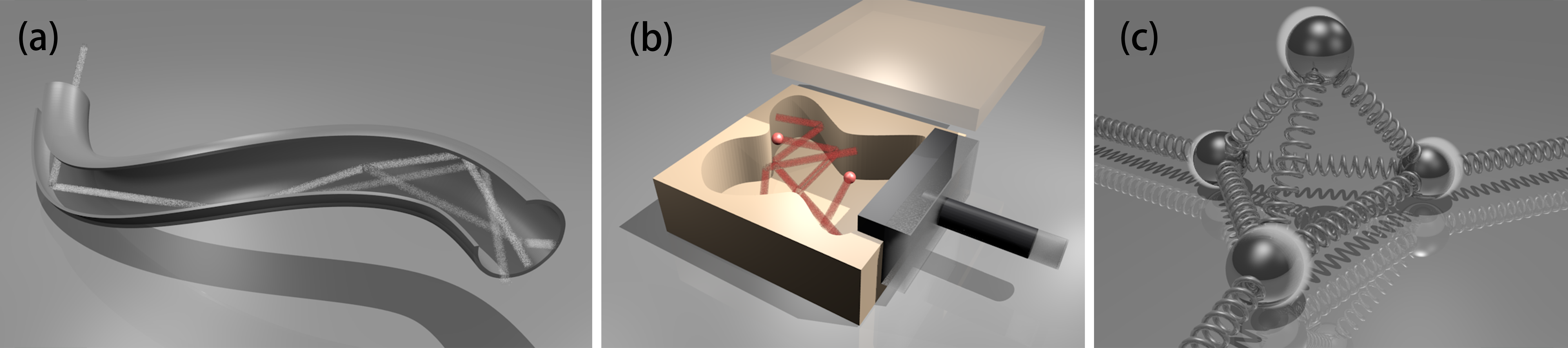
Figure 1: (Color online) Schematics of various multi-mode systems in the presence of noisy environment: (a) A MMF experiencing twists, bendings, and other forms of perturbations along the propagation direction $z$; (b) A multi-mode quantum dot (or a multi-mode opto-mechanical cavity) with an incoherently moving wall; (c) random network of coupled mechanical oscillators (slow envelope approximation) in the presence of noisy environment.

Outline.– In this paper we utilize a Random Matrix Theory (RMT) approach in order to unveil a physical mechanism that shields wave coherent effects in the presence of disorder. The RMT approach typically uncovers the most universal properties of wave transport in complex systems, and it can therefore serve as a good starting point for the understanding of designing schemes that protect the wave nature of propagation against noise. Specifically, we analyze the decay of an initial mode excitation (labeled $n_{0}$) in MMF that consist of $N$ modes with propagation constants $\beta_{n}=n\Delta$ where ${n=1,\cdots,N}$. The main objective is to study the decay of the survival probability $\mathcal{P}(z)$ towards its ergodic limit $\sim 1/N$. The mode mixing is due to quenched disorder associated with external perturbations along the propagation direction $z$ of the MMF. It is characterized by its strength $\varepsilon$ and by a correlation length $z_{c}$. From practical as well as physical point of view the interest is mainly in weak disorder ($\varepsilon<\sqrt{N}\Delta$), that can be characterized by a Fermi-Golden-Rule rate

$$\Gamma\ =\ \frac{4\pi}{\Delta}\varepsilon^{2}$$ (1)

Consequently we distinguish between two length scales:

$$z_{\Delta}\equiv\frac{2\pi}{N\Delta};\quad\quad z_{\Gamma}\equiv\frac{1}{\Gamma}$$ (2)

The former is the short length scale over which the bandwidth is resolved, while the latter characterizes the non-stochastic coherent decay of an excitation. We distinguish between short correlation length ($z_{c}<z_{\Delta}$) and long correlation length ($z_{c}>z_{\Gamma}$). In the latter regime we find ballistic-like decay $\mathcal{P}(z)\sim 1/z$ as opposed to the exponential decay for shorter $z_{c}$. In the concluding paragraph we emphasize that the results of our study are relevant for a wide range of multi-mode or multi-level physical settings (see Fig. 1), appearing in areas as diverse as mesoscopic optics, and matter waves to quantum electronics and quantum biology.

RMT modeling.– We presume that the perturbations along the propagation distance of the fiber induce only coupling between forward propagating modes (paraxial approximation). Furthermore, we consider that the fiber can be described in terms of concatenated segments of length $z_{c}$ which are associated with statistically independent fiber perturbations. Based on these assumptions we can write a paraxial Hamiltonian $H^{(k)}=H_{0}+\varepsilon B^{(k)}$ that describes the field propagation within the $k$-th segment. Here $H_{0}$ describes the unperturbed fiber and $B^{(k)}=\left(B^{(k)}\right)^{\dagger}$ represents the perturbation of the $k$-th segment that is responsible for the mode mixing. In the mode representation the $N\times N$ matrix $H_{0}$ is diagonal with elements ${H_{nm}^{(0)}=\beta_{n}\delta_{n,m}}$. For simplicity we assume that the mode propagation constants are equally spaced, namely $\beta_{n}=n\Delta$ where ${n=1,\cdots,N}$. The perturbation matrix $B^{(k)}$ is modeled as a GUE random matrix. For such matrix $\langle|B|^{2}\rangle=2$, hence the off diagonal terms of the Hamiltonian have dispersion $2\varepsilon^{2}$ and zero average. Note that this factor of 2 is reflected in the definition of Eq.​​ (1).

The field propagation in each section $k$ is described by the unitary matrix

$$U^{(k)}\ =\ e^{-i\left(H_{0}+\varepsilon B^{(k)}\right)z_{c}}$$ (3)

In the analysis below, we do not consider polarization degrees of freedom. It can be shown that their presence does not alter the general picture (appart from an abrupt drop in the survival probability during the first evolution step), and therefore we omit them for a better clarity of the presentation. Below, unless stated otherwise, we assume that the paraxial distances are measured in units of mean propagation constant spacing $\Delta$.

The one step dynamics is characterized by a stochastic kernel

$$P(n|n_{0})\ = \ \overline{\left|\left\langle n\middle|U^{(k)}\middle|n_{0}\right\rangle\right|^{2}}$$ (4)

$$\equiv \ (1{-}\lambda)\delta_{n,n_{0}}+\lambda W(n-n_{0})$$ (5)

Here we averaged the one-step dynamics over realizations of the random matrix $B^{(k)}$. The parameter $\lambda$ is defined as the probability that is drained from the initial mode after one step. The function $W(n-n_{0})$ describes the distribution of the probability over the other modes. The modal field amplitudes $\Psi_{n}(z)$ at distance $z$ along the MMF are determined by operating on the initial state ${\Psi_{n}(0)=\delta_{n,n_{0}}}$ with an ordered sequence of $U^{(k)}$ matrices (${k=1,2,\cdots}$). This multi-step dynamics generates a distribution ${P_{z}(n|n_{0})=|\Psi_{n}(z)|^{2}}$. Below we discuss how ${P_{z}(n|n_{0})}$ is related to ${P(n|n_{0})}$, and what are the implications regrading the survival probability

$$\mathcal{P}(z)\ \ \equiv\ \ P_{z}(n_{0}|n_{0})$$ (6)

Short correlation length.– For short segment ($z<z_{\Delta}$) the probability that is transferred to each of the $N$ modes is $2\varepsilon^{2}z_{c}^{2}$ hence the total probability that is drained from the initial mode is

$$\lambda\ =\ N\times 2\varepsilon^{2}z_{c}^{2}\ =\ \frac{z_{c}^{2}}{z_{\Gamma}z_{\Delta}}$$ (7)

As long as the first term in Eq.​​ (5) dominates, successive convolutions lead to exponential decay, namely, after $t$ steps ${(1{-}\lambda)^{t}\approx\exp(-\lambda t)}$, with $t=z/z_{c}$, hence

$$\mathcal{P}(z)\ =\ \exp\left[-\frac{\ z_{c}}{z_{\Delta}z_{\Gamma}}z\right],\ \ \ \ \mbox{for $z_{c}<z_{\Delta}$}$$ (8)

The above has been tested numerically and was found to reproduce nicely the results of our simulations for various $N$-values, see Fig. 2a. At the same figure we also display the single step $P(n|n_{0})$, and the $P_{z}(n|n_{0})$ distribution after 100 steps, see Fig. 2b and Fig. 2c respectively. In both instances the shape of the evolving distribution is dominated by a delta peak around the initial mode ($n_{0}=N/2$). This delta peak is gradually drained, until it attains the ergodic value ${\mathcal{P}(z)\approx 1/N}$.

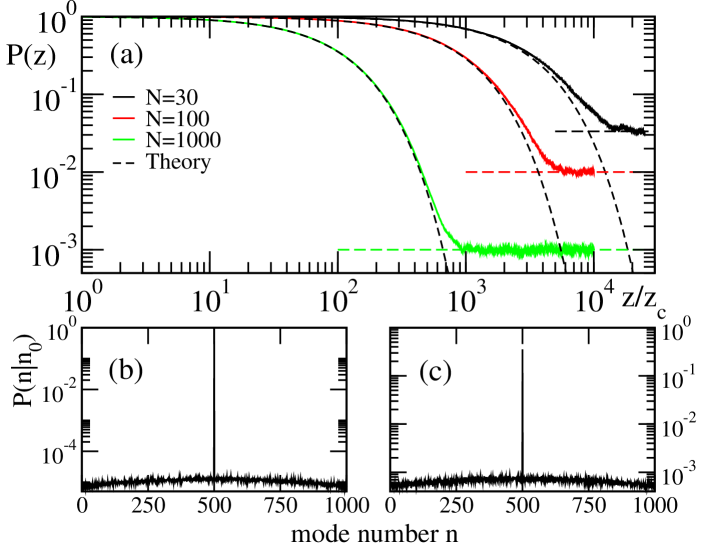
Figure 2: (Color online) (a) The decay of the survival probability for short correlation lengths $z_{c}=0.005$, and perturbation strength $\varepsilon=0.5$. The units are chosen such that $\Delta=1$. The various colored curves indicate MMFs with different number of modes $N=30,100,1000$. The colored horizontal dashed lines indicate the ergodic value ${\mathcal{P}(z)\approx 1/N}$. The black dashed lines indicate Eq.(8); (b) The coherent spreading $P(n|n_{0})$ for $z=z_{c}$; (c) The spreading profile $P_{z}(n|n_{0})$ for $z=100z_{c}$.

Large correlation length.– For $z_{c}>z_{\Gamma}$ it is well known from the study of the coherent dynamics CIK00 ; Mello97 that the initial delta peak completely dissolves, and one obtains Eq.​​ (5) with $\lambda\sim 1$ and Lorentzian line shape

$$W(n-n_{0})=\frac{\Delta}{\pi}\frac{\Gamma}{[(n-n_{0})\Delta]^{2}+\Gamma^{2}}$$ (9)

This line shape is obtained after distance $z_{\Gamma}$. After a larger distance $z_{c}>z_{\Gamma}$ the line shape does not change, but the phases of the wavefunction are further randomized. It follows that the coherent evolution over successive segments can be approximated as a convolution of $W(n^{\prime}-n^{\prime\prime})$ kernels. We therefore get effectively stochastic evolution. But this stochastic evolution does not obey the central limit theorem. It is of the Levy-flight type because the Lorentzian does not have a finite second moment. Successive convolutions of $t=z/z_{c}$ Lorentzians give a wider Lorentzian of width $\Gamma t$. It follows from Eq.​​ (9) that the survival provability decays in a ballistic-like fashion:

$$\mathcal{P}(z)\ =\ 2\frac{z_{\Gamma}z_{c}}{Nz_{\Delta}}\frac{1}{z},\ \ \ \ \mbox{for $z_{c}>z_{\Gamma}$}$$ (10)

The above picture is nicely confirmed by our detailed numerical analysis. In Fig. 3a we report our findings for the survival probability for various mode sizes $N$, and perturbations strengths $\varepsilon$. In Fig. 3b we also report the Lorentzian waveform at the end of the coherent evolution $z=z_{c}$. The robustness of the Lorentzian shape Eq. (9) against the dynamical disorder is further confirmed in Fig. 3c where we plot $P_{z}(n|n_{0})$ after $5$ segments.

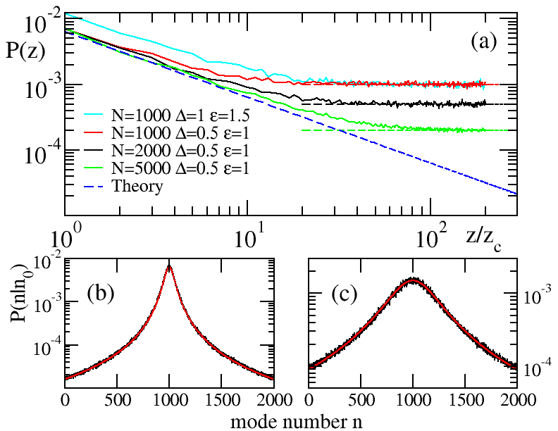
Figure 3: (Color online) (a) The decay of the survival probability for large correlation length $z_{c}=0.32$. The various colored curves indicate MMFs with different parameters as indicated in the figure legend. The horizontal dashed lines indicate the ergodic limit ${\mathcal{P}(z)\approx 1/N}$. The blue dashed line indicates Eq.(10). (b) The coherent spreading $P(n|n_{0})$ for $z=z_{c}$; (c) The spreading profile $P_{z}(n|n_{0})$ for $z=5z_{c}$. In both (b,c) the parameters are $\Delta=0.5$, $\varepsilon=1$ and $N=2000$ while the red dashed line indicates the Lorentzian of Eq.(9).

Intermediate correlation length.– Consider $z_{\Delta}<z_{c}<z_{\Gamma}$. In this case, the initial spreading is dictated by a Fermi-Golden-Rule (FGR) type picture. Namely, the probability that is transferred to each of the modes within the unresolved bandwidth $2\pi/z_{c}$ is $(\varepsilon z_{c})^{2}$, hence the total probability that is drained from the initial mode is

$$\lambda\ \ =\ \ \Gamma z_{c}$$ (11)

The analysis proceeds as in the discussion of short correlation scale, just with this different expression for $\lambda$. Namely, as long as the first term in Eq.​​ (5) dominates, successive convolutions lead to exponential decay ${\exp(-\lambda t)}$ with $t=z/z_{c}$. Consequently we obtain a result that is independent of $z_{c}$, namely,

$$\mathcal{P}(z)\ =\ \exp\left[-\frac{1}{z_{\Gamma}}z\right],\ \ \ \ \mbox{for $z_{\Delta}<z_{c}<z_{\Gamma}$}$$ (12)

Equation (12) compares nicely with the numerical simulations, see Fig. 4a. Notice that as opposed to Eq. (8), now the decay rate does not involve the number of modes of the system $N$ and neither depends on $z_{c}$. At the same time the envelope of the evolving waveform acquires Lorentzian-like tails spilled all over the $N$ modes, see Fig. 4b. Nevertheless, the dominant component of the waveform is centered at the initial mode $n_{0}$. For larger propagation distances $z>z_{\Gamma}$, the FGR decay law Eq. (12) cease to apply. Instead, either the waveform reach an ergodic distribution (see the black line in Fig. 4a, corresponding to $N=10$) or (in the case of large number of modes $N$) it continues spreading; albeit with a different form. Specifically, the previous argument associated with the robustness of the Lorentzian waveform against noise takes over, and we recover the physics that led us to Eqs. (9,10), see Fig. 4a,c.

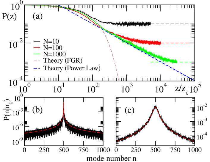
Figure 4: (Color online) (a) The decay of the survival probability for intermediate correlation length $z_{c}=1$, and perturbation strength $\varepsilon=0.05$. The units are chosen such that $\Delta=1$. The various colored curves indicate MMFs with different number of modes ${N=10,100,1000}$. The color horizontal dashed lines indicate the ergodic limit ${\mathcal{P}(z)\approx 1/N}$. The brown dashed line indicates the FGR exponential decay Eq.(12), while the blue dashed line indicates the power-law decay Eq.(10). (b) The coherent spreading $P(n|n_{0})$ for $z=z_{c}$; (c) The spreading profile $P_{z}(n|n_{0})$ for $z=1000z_{c}$. In both (b,c) the parameters are $\Delta=1$, $\varepsilon=0.05$ and $N=1000$ while the red dashed line indicates the Lorentzian of Eq.(9).

Strong disorder, diffusive decay.– So far we have discussed weak disorder. We now turn to discuss briefly the strong disorder regime ($\varepsilon>\sqrt{N}\Delta$). The scenario for short ${z_{c}}$ is formally the same as that of the “short correlation” analysis, leading to an exponential decay. But if $z_{c}$ exceeds ${z_{N}=1/(\sqrt{N}\varepsilon)}$ the probability is drained from the initial mode, and the distribution becomes ergodic with ${\mathcal{P}(z)\approx 1/N}$. At this stage one wonders why the naively expected diffusive decay does not appear. Are we missing something in the analysis? The answer is that the analysis so far has assumed $B$ that looks like a full GUE matrix. But in more general circumstance $B$ might have a finite bandwidth ${b\ll N}$. The analysis for the weak disorder regime still holds but with $N$ replaced by $b$. In contrast, in the strong disorder regime, it is well known CIK00 that the saturation profile is not a Lorentzian. Rather, if $z_{c}$ is long enough, the saturation profile is exponentially localized over ${\xi=b^{2}}$ modes. Such saturation profile has a finite second moment. Consequently, the same argumentation as in the “long correlation regime” implies that the width of the distribution evolves as $\xi\sqrt{t}$, where $t=z/z_{c}$ is the number of steps. This leads to the conclusion that the survival provability decays in a diffusive-like fashion:

$$\mathcal{P}(z)\ \approx\ \frac{1}{b^{2}}\sqrt{\frac{z_{c}}{z}}$$ (13)

Because of lack of space, we defer a more detail discussion of other results and a thorough analysis of the decay of the survival probability for the more realistic case where $b\ll N$ to a later publication LCK19 .

Summary – We have illuminated the interplay between the short time coherent evolution and the long time stochastic spreading in multimode systems. The correlation scale $z_{c}$ of a disordered environment determines the crossover from an exponential-decay to diffusive- like or ballistic-like decay. The latter is due to a Levy-type spreading which is implied by convolution of Lorentzian kernels. Our results have been formulated using a universal RMT modeling. A future direction that we currently pursue LCK19 is to design other coupling schemes for which the one-step coherent evolution leads to tailored anomalous decay of the survival probability.

Acknowledgments – (Y.L) and (T.K) acknowledge partial support by an AFOSR grant No. FA 9550-10-1-0433, and by an NSF grant EFMA-1641109. Y.L. acknowledge funding from the Wesleyan University CIS summer research program. (D.C.) acknowledges support by the Israel Science Foundation (Grant No. 283/18). The authors acknowledge useful discussions with E. Makri and Y. Cai who participated at the initial stage of the project.

References

- (1) K. Southwell, Quantum coherence, Nature 453, 1003 (2008) [and articles therein].
- (2) J. P. Dowling, G. J. Milburn, Quantum technology: the second quantim revolution, Phil. Trans. R. Soc. Lond. A 361, 1655 (2003).
- (3) E. Andersson, P. Öhberg, Quantum Information and Coherence, Springer (2014)
- (4) D. V. Averin, B. Ruggiero, P. Silvertrini, macroscopic Quantum Coherence and Quantum Computing, Springer (2001).
- (5) G. S. Engel, T. R. Calhoun, E. L. Read, T-K Ahn, T. Mancal, Y-C Cheng, R. E. Blankenship, G. R. Fleming, Evidence for wavelike energy transfer through quantum coherence in photosynthetic systems, Nature 446, 782 (2007).
- (6) G. Panitchayangkoona, D. Hayesa, K. A. Fransteda, J. R. Carama, E. Harela, J. Wenb, R. E. Blankenshipb, G. S. Engela, Long-lived quantum coherence in photosynthetic complexes at physiological temperature, PNAS 107, 12766 (2010)
- (7) M. Sarovar, A. Ishizaki, G. R. Fleming, K. B. Whaley, Quantum entanglement in photosynthetic light-harvesting complexes, Nature Physics 6, 462 (2010)
- (8) Seth Lloyd, Quantum coherence in biological systems, J. Phys.: Conf. Ser. 302, 012037 (2011).
- (9) G. S. Engel, Quantum Coherence in Photosynthesis, Procedia Chemistry 3, 222 (2011).
- (10) G. R. Fleming, G. D. Scholes, Y-C Cheng, Quantum Effects in biology, Procedia Chemistry 3, 38 (2011).
- (11) Y. Zhang, G. L. Celardo, F. Borgonovi, L. Kaplan, Opening-assisted coherent transport in the semiclassical regime, Phys. Rev. E 95, 022122 (2017)
- (12) G. Keiser, Optical Fiber Communications, third ed., McGraw-Hill, 2000.
- (13) B. Redding, M. Alam, M. Seifert, and H. Cao, “High-resolution and broadband all-fiber spectrometers,” Optica 1, 175 (2014).
- (14) W. Xiong, P. Ambichl, Y. Bromberg, B. Redding, S. Rotter, and H. Cao, Spatiotemporal control of light transmission through a multimode fiber with strong mode mixing, Phys. Rev. Lett. 117, 053901 (2016).
- (15) K-P Ho, J. M. Kahn, Mode Coupling and its Impact on Spatially Multiplexed Systems, Optical Fiber Telecommunications VIB, Elsevier (2013).
- (16) W. Xiong, P. Ambichl, Y. Bromberg, B. Redding, S. Rotter, and H. Cao, Principal modes in multimode fibers: exploring the crossover from weak to strong mode coupling, Opt. Express 25, 2709 (2017).
- (17) D. Cohen, T. Kottos, Parametric dependent Hamiltonians, wave functions, random matrix theory, and quantal-classical correspondence, Phys. Rev. E 63, 036203 (2001)
- (18) D. Cohen, F. M. Izrailev, T. Kottos, Wave packet dynamics in energy space, random matrix theory, and the quantum- classical correspondence, Phys. Rev. Lett. 84, 2052-2055 (2000).
- (19) J. L. Gruver, J. Aliaga, H. A. Cerdeira, P. Mello, A. N. Proto, Energy-level statistics and time relaxation in quantum systems, Phys. Rev. E 55, 6370 (1997)
- (20) Y. Li, D. Cohen, T. Kottos, in preparation (2019).