Dynamic Sparse Factor Analysis

Abstract

Its conceptual appeal and effectiveness has made latent factor modeling an indispensable tool for multivariate analysis. Despite its popularity across many fields, there are outstanding methodological challenges that have hampered practical deployments. One major challenge is the selection of the number of factors, which is exacerbated for dynamic factor models, where factors can disappear, emerge, and/or reoccur over time. Existing tools that assume a fixed number of factors may provide a misguided representation of the data mechanism, especially when the number of factors is crudely misspecified. Another challenge is the interpretability of the factor structure, which is often regarded as an unattainable objective due to the lack of identifiability. Motivated by a topical macroeconomic application, we develop a flexible Bayesian method for dynamic factor analysis (DFA) that can simultaneously accommodate a time-varying number of factors and enhance interpretability without strict identifiability constraints. To this end, we turn to dynamic sparsity by employing Dynamic Spike-and-Slab (DSS) priors within DFA. Scalable Bayesian EM estimation is proposed for fast posterior mode identification via rotations to sparsity, enabling Bayesian data analysis at scales that would have been previously time-consuming. We study a large-scale balanced panel of macroeconomic variables covering multiple facets of the US economy, with a focus on the Great Recession, to highlight the efficacy and usefulness of our proposed method.

Keywords: Dynamic Sparsity, Factor Analysis, Spike-and-Slab, Time Series.

1 Introduction

The premise of dynamic factor analysis (DFA) is fairly straightforward: there are unobservable commonalities in the variation of observable time series, which can be exploited for interpretation, forecasting, and decision making. Dating back to, at least, Burns and Mitchell (1947), the fundamental idea that a small number of indices drive co-movements of many time series has found plentiful empirical support across a wide range of applications including economics (Stock and Watson, 2002; Bai and Ng, 2002; Bernanke et al., 2005; Baumeister et al., ; Cheng et al., 2016), finance (Diebold and Nerlove, 1989; Aguilar et al., 1998; Pitt and Shephard, 1999; Aguilar and West, 2000; Carvalho et al., 2011), and ecology (Zuur et al., 2003), to name just a few. More notably, in their seminal work on DFA, Sargent et al. (1977) showed that two dynamic factors could explain a large fraction of the variance of U.S. quarterly macroeconomic variables. Motivated by a similar (but significantly larger) application, we develop scalable Bayesian DFA methodology and deploy it to glean insights into the hidden drivers of the U.S. macroeconomy before, during and after the Great Recession.

With large-scale cross sectional data becoming readily available, the need for developing scalable and reliable tools adept at capturing complex latent dynamics have spurred in both statistics and econometrics (Beyeler and Kaufmann, 2016; Kaufmann and Schumacher, 2017; Fruehwirth-Schnatter and Lopes, 2018; Nakajima et al., 2017). While “dynamic factor models have been the main big data tool used over the past 15 years by empirical macroeconomists” (Stock and Watson, 2016), there are remaining methodological challenges. It is now commonly agreed that high-dimensional inference can hardly be formalized and executed without any sparsity assumptions. The fundamental goal of our research is to facilitate sparsity discovery (i.e. data-informed sparsity), when in fact present. In doing so, we keep in mind three main pillars that we regard as essential for building a stable foundation for sparse factor modeling.

Firstly, the latent factor loadings should account for time-varying patterns of sparsity. In (macro-)economics and finance, the sequentially observed variables may go through multiple periods of shocks, expansions, and contractions (Hamilton, 1989). It is thus expected that the underlying latent structure changes over time– either gradually or suddenly– where some factors might be active at all times, while others only at certain times. For example, in our empirical analysis we find that certain factors exert influence on some series only during a crisis and later permeate through different components of the economy as the shock spreads. Dynamic sparsity plays a very compelling role in capturing and characterizing such dynamics. Recent developments in sparse factor analysis reflect this direction of interest (West, 2003; Carvalho et al., 2008; Yoshida and West, 2010; Lopes et al., 2010). More recently, Nakajima and West (2013b) deployed the latent threshold approach of Nakajima and West (2013a) in order to induce zero loadings dynamically over time. Our methodological contribution builds on this development, but poses far less practical limitations on the dimensionality of the data and far less constraints on identification.

Related to the previous point is the question of selecting the number of factors. This modeling choice is traditionally determined by a combination of a priori knowledge, a visual inspection of the scree plot (Onatski, 2009), and/or information criteria (Bai and Ng, 2002; Hallin and Liska, 2007). In the presence of model uncertainty, the Bayesian approach affords the opportunity to assign a probabilistic blanket over various models. Bayesian non-parametric approaches have been considered for estimating the factor dimensionality using sparsity inducing priors (Bhattacharya and Dunson, 2011; Rockova and George, 2016). The added difficulty stemming from time series data, however, is that the number of factors may change over time. Despite plentiful empirical evidence for this behavior in macroeconomic data (Bai and Ng, 2002), the majority of existing DFA tools treat the number of factors as fixed over time. As a remedy, we turn to dynamic sparsity as a compass for determining the number of factors without necessarily committing to one fixed number ahead of time.

The third essential requirement is accounting for structural instabilities over time with time-varying loadings and/or factors. One seemingly simple solution has been to deploy rolling/extending window approaches to obtain pseudo-dynamic loadings. These estimates, however, lack any supporting probabilistic structure that would induce smoothness and/or capture sudden dynamics. Recent DFA developments (Del Negro and Otrok, 2008; Nakajima and West, 2013a) have treated both the factors and loadings as stochastic and dynamic. Adopting this point of view, we blend smoothness with sparsity via Dynamic Spike-and-Slab (DSS) priors on factor loadings (Rockova and McAlinn, 2017). This prior regards factor loadings as arising from a mixture of two states: an inactive state represented by very small loadings and an active state represented by smoothly evolving large loadings. The mixing weights between these two states themselves are time-varying, reflecting past information to prevent from erratic regime switching. The DSS priors allow latent factors to effectively, and smoothly, appear or disappear from each series, tracking the evolution of sparsity over time.

In this work, we develop methodology for sparse dynamic factor analysis that is built on the three foundational principles mentioned above. Using this methodology, we examine a large-scale balanced panel of macroeconomic indices that span multiple corners of the U.S. economy from 2001 to 2015. Our method helps understand how the economy evolves over time and how shocks affect its individual components. In particular, examining the latent factor structure before, during, and after the Great Recession, we obtain insights into the channels of dependencies and we assess permanence of structural changes.

To ensure that our implementation scales with large datasets, we propose an EM algorithm for MAP estimation that recovers evolving sparse latent structures in a fast and potent manner. As the EM algorithm finds a likely sparse structure, it does not require strong identification constraints that would be needed for MCMC simulation. While interpretation can be achieved with ex-post rotations (Bai and Ng, 2013; Kaufmann and Schumacher, 2017), here we deploy rotations to sparsity inside the EM algorithm along the lines of Rockova and George (2016) to (a) accelerate convergence and (b) obtain better oriented sparse solutions.

The paper is structured as follows. Section 2 outlines the dynamic sparse factor model. Section 3 summarizes our EM estimation strategy. A detailed simulation study that highlights our strategy relative to other methods is in Section 4. An empirical study on a large-scale macroeconomic dataset is in Section 5. We conclude the paper with additional comments in Section 6. Details of the implementation are in the Supplementary Materials.

2 Dynamic Sparse Factor Models

The data setup under consideration consists of a matrix of high-dimensional multivariate time series $\boldsymbol{Y}=[\boldsymbol{Y}_{1},\dots,\boldsymbol{Y}_{T}]\in\mathbb{R}^{P\times T}$, where each vector $\boldsymbol{Y}_{t}\in\mathbb{R}^{P}$ contains a snapshot of continuous measurements at time $t$. Dynamic factor models are built on the premise that there are only a few latent factors that drive the co-movements of $\boldsymbol{Y}_{t}$. Evolving covariance patterns of time series can be captured with the following state space model:

$$\boldsymbol{Y}_{t} =\boldsymbol{B}_{t}\boldsymbol{\omega}_{t}+\mbox{\boldmath$\epsilon$}_{t},\quad\mbox{\boldmath$\epsilon$}_{t}\stackrel{{\scriptstyle ind}}{{\sim}}\mathcal{N}_{P}(\mbox{\boldmath$0$},\mbox{\boldmath$\Sigma$}_{t}),$$ (1)

$$\boldsymbol{\omega}_{t} =\mbox{\boldmath$\Phi$}\boldsymbol{\omega}_{t-1}+\boldsymbol{\mathrm{e}}_{t},\quad\boldsymbol{\mathrm{e}}_{t}\stackrel{{\scriptstyle ind}}{{\sim}}\mathcal{N}_{K}(\mbox{\boldmath$0$},\,\sigma^{2}_{\omega}\mathbb{I}_{K}),$$ (2)

which extends the more standard dynamic factor models (Sargent et al., 1977; Geweke, 1977) in at least two ways. First, the observation equation (1) links $\boldsymbol{Y}_{t}$ to a vector of factors $\boldsymbol{\omega}_{t}$ through multivariate regression with loadings $\boldsymbol{B}_{t}\in\mathbb{R}^{P\times K}$ and with residual variances $\mbox{\boldmath$\Sigma$}_{t}=\mathrm{diag}\{\sigma_{1t}^{2},\dots,\sigma_{Pt}^{2}\}$, where both $\boldsymbol{B}_{t}$ and $\mbox{\boldmath$\Sigma$}_{t}$ are dynamic, i.e. are allowed to evolve over time. In this section, we tacitly assume that any location shifts in $\boldsymbol{Y}$ have been standardized away and thereby we omit an intercept in (1). The (dynamic) intercept can be however included, as we demonstrate in Section 5. Second, the transition equation (2) describes the unobserved regressors $\boldsymbol{\omega}_{t}$ as following a stationary autoregressive process with a transition matrix $\mbox{\boldmath$\Phi$}=\widetilde{\phi}\,\mathbb{I}_{K}$ for some $0<\widetilde{\phi}<1$ and with Gaussian disturbances $\boldsymbol{\mathrm{e}}_{t}$ with a known variance $\sigma^{2}_{\omega}>0$. As is customary with state-space models of this type, we assume that $\boldsymbol{\omega}_{t},$ $\boldsymbol{\mathrm{e}}_{t}$ and $\mbox{\boldmath$\epsilon$}_{t}$ are cross-sectionally independent.

A related approach was proposed in Aguilar and West (2000) and Lopes and Carvalho (2007), who also permit time-varying loadings, but do not impose the AR(1) process on the factors. Instead, their factors are cross-sectionally independent and linked over time through a stochastic volatility evolution of their idiosyncratic variances. Bai and Ng (2002) and Stock and Watson (2010), on the other hand, assume that factors follow vector autoregression, but the loadings are constant over time. As in Nakajima and West (2013b), our model (1) and (2) differs from these more standard dynamic factor model formulations because it combines the AR(1) factor aspect together with dynamic loadings.

The equations (1) and (2) imply that, marginally, $\boldsymbol{Y}_{t}\sim\mathcal{N}_{P}(0,\widetilde{\mbox{\boldmath$\Sigma$}}_{t})$, where $\widetilde{\mbox{\boldmath$\Sigma$}}_{t}=\sigma^{2}_{\omega}/(1-\widetilde{\phi}^{2})\boldsymbol{B}_{t}\boldsymbol{B}_{t}^{\prime}+\mbox{\boldmath$\Sigma$}_{t}$. This decomposition provides a fundamental justification for factor-based dynamic covariance modeling. The information in high-dimensional vectors $\boldsymbol{Y}_{t}$ is distilled through latent factors into lower-dimensional factor loadings matrices $\boldsymbol{B}_{t}$, which completely characterize the movements of covariances over time. Other authors (Del Negro and Otrok, 2008; Lopes and Carvalho, 2007) consider a stochastic volatility (SV) evolution (either log-AR(1) or Bayesian discounting) on the variance of the latent factors and/or the innovations $\mbox{\boldmath$\epsilon$}_{t}$ in (1). While both are feasible within our framework, here we impose Bayesian discounting SV formulation on the innovation variances: $\sigma_{jt}=\sigma_{jt-1}\delta/\upsilon_{jt},$ where $\delta\in(0,1]$ is a discount parameter and where $\upsilon_{jt}\sim\mathcal{B}(\delta\eta_{t-1}/2,(1-\delta)\eta_{t-1}/2)$ with $\eta_{t}=\delta\eta_{t-1}+1$ (Ch. 4.3.7 Prado and West, 2010).

Parsimonious covariance estimation is only one of the objectives of dynamic factor modeling. The more traditional objective is disentangling the covariance structure and understanding its driving forces and how they change over time. Sparse modeling has been indispensable for both of these objectives, where fewer estimable coefficients yield far more stable covariance estimates and where nonzero patterns in $\boldsymbol{B}_{t}$ yield superior interpretable characterizations (Carvalho et al., 2008; Yoshida and West, 2010). Next, we explore the role of dynamic sparsity in DFA.

2.1 Dynamic Sparsity with Shrinkage Process Priors

No assumption has been as pervasive in the analysis of high-dimensional data as the one of sparsity. Sparsity is a practical modeling choice that facilitates high-dimensional inference and/or computation. In factor model contexts, it can also be used to anchor on identifiable parametrizations (Fruhwirth-Schnatter and Lopes, 2009) and/or for estimating factor dimensionality (Rockova and George, 2016; Bhattacharya and Dunson, 2011). The potential of sparsity in dynamic factor models has begun to be recognized (Nakajima and West, 2013b; Beyeler and Kaufmann, 2016; Kaufmann and Schumacher, 2017).

In this work, we complement the factor model formulation (1) with dynamic sparsity priors on the factor loadings $\boldsymbol{B}_{t}$ for $1\leq t\leq T$. In other words, rather than imposing a dense model by assigning a random walk (or a stationary autoregressive) prior on the loadings (such as Stock and Watson, 2002; Del Negro and Otrok, 2008), we allow for the possibility that the loadings are zero at certain times.

We will write $\boldsymbol{B}_{t}=(\beta_{jk}^{t})_{j,k=1}^{P,K}$ and impose a shrinkage process prior on individual time series $\{\beta_{jk}^{t}\}_{t=1}^{T}$ for each $(j,k)$. A few authors have reported on the benefits of dynamic variable selection in the analysis of macroeconomic data (Frühwirth-Schnatter and Wagner, 2010; bitto2016achieving; Lopes et al., 2010; Nakajima and West, 2013b; Koop et al., 2010). We build on one of the more recent developments, the Dynamic Spike-and-Slab (DSS) priors proposed by Rockova and McAlinn (2017).

DSS priors are dynamic extensions of spike-and-slab priors for variable selection (George and McCulloch, 1993; Rockova and George, 2018). Each coefficient in DSS is thought of as arising from two latent states: (1) an inactive state, where the coefficient meanders randomly around zero, and (2) an active state, where the coefficient walks on an autoregressive path. The switching between these two states is driven by a dynamic mixing weight which depends on past values of the series, making the states less erratic over time.

We begin by reviewing the conditional specification of the DSS prior. For each coefficient $\beta_{jk}^{t}$, we have a binary indicator $\gamma_{jk}^{t}\in\{0,1\}$, which encodes the state of $\beta_{jk}^{t}$ (the “spike” inactive state for $\gamma_{jk}^{t}=0$ and the “slab” active state for $\gamma_{jk}^{t}=1$). Given $\gamma_{jk}^{t}$ and a lagged value $\beta_{jk}^{t-1}$, we assume a conditional mixture prior (independently for each $(j,k)$):

$$\pi(\beta_{jk}^{t}|\gamma_{jk}^{t},\beta_{jk}^{t-1})=(1-\gamma_{jk}^{t})\psi_{0}(\beta_{jk}^{t}|\lambda_{0})+\gamma_{jk}^{t}\psi_{1}\left(\beta_{jk}^{t}\,|\,\mu(\beta_{jk}^{t-1}),\lambda_{1}\right),$$ (3)

where

$$\mu(\beta_{jk}^{t-1})=\phi_{0}+\phi_{1}(\beta_{jk}^{t-1}-\phi_{0})\quad\text{with}\quad|\phi_{1}|<1$$ (4)

and

$$\mathbb{P}(\gamma_{jk}^{t}=1|\beta_{jk}^{t-1})=\theta_{jk}^{t}.$$ (5)

The conditional prior (3) is a mixture of two components: (i) a spike Laplace density $\psi_{0}(\beta|\lambda_{0})$ that is concentrated around zero and (ii) a Gaussian slab density $\psi_{1}(\beta_{t}|\mu(\beta_{jk}^{t-1}),\lambda_{1})$, which is moderately peaked around its mean $\mu(\beta_{jk}^{t-1})$ with variance $\lambda_{1}$. This mixture formulation is an extension of existing continuous spike-and-slab priors (George and McCulloch, 1993; Ishwaran et al., 2005; Rockova, 2018), allowing the mean $\mu(\beta_{jk}^{t-1})$ of the non-negligible coefficients to evolve smoothly over time (through a stationary autoregressive process). The spike distribution $\psi_{0}(\beta_{t}|\lambda_{0})$, on the other hand, does not depend on $\beta_{jk}^{t-1}$, effectively shrinking the negligible coefficients towards zero. In this regard, the conditional prior in (3) can be seen as a “multiple shrinkage” prior (George, 1986b, a) with two centers of gravity.

In time series data (as will be seen from our empirical study), it reasonable to expect that some factors are active only for some periods of time. Such “pockets of predictability” (Farmer et al., 2018) can be captured with spike/slab memberships $\gamma_{jk}^{t}$ that evolve somewhat smoothly. This behavior can be encouraged with dynamic mixing weights $\theta_{jk}^{t}$ (defined in (5)) that reflect past information. To this end, we deploy the deterministic construction of Rockova and McAlinn (2017) defined, for some global balancing parameter $0<\Theta<1$, as follows

$$\theta_{jk}^{t}\equiv\theta(\beta_{jk}^{t})=\frac{\Theta\psi_{1}^{ST}\left(\beta_{jk}^{t}|\lambda_{1},\phi_{0},\phi_{1}\right)}{\Theta\psi_{1}^{ST}\left(\beta_{jk}^{t}|\lambda_{1},\phi_{0},\phi_{1}\right)+(1-\Theta)\psi_{0}\left(\beta_{jk}^{t}|\lambda_{0}\right)},$$ (6)

given $(\Theta,\lambda_{0},\lambda_{1},\phi_{0},\phi_{1})$. This mixing weight has an interesting interpretation. It is defined as the marginal inclusion probability $\mathbb{P}(\gamma_{jk}^{t-1}=1\,|\>\beta_{jk}^{t-1})$ for classifying $\beta_{jk}^{t-1}$ as arising from the stationary slab distribution $\psi_{1}^{ST}\left(\beta_{jk}^{t}|\lambda_{1},\phi_{0},\phi_{1}\right)$, as opposed to the stationary spike distribution $\psi_{0}\left(\beta_{jk}^{t}|\lambda_{0}\right)$, under the prior $\mathbb{P}(\gamma_{jk}^{t-1}=1)=\Theta$. As $\theta_{jk}^{t}$’s evolve over time, they project the latent state (active/inactive) of the past value onto the next values. These weights induce marginal stability in the sense that each coefficient $\beta_{jk}$ has a marginal spike-and-slab distribution, i.e. $\pi(\beta_{jk})=\Theta\psi_{1}^{ST}\left(\beta_{jk}^{t}|\lambda_{1},\phi_{0},\phi_{1}\right)+(1-\Theta)\psi_{0}\left(\beta_{jk}^{t}|\lambda_{0}\right)$ (see Theorem 1 of Rockova and McAlinn, 2017).

Having introduced the DSS priors, we can now fully specify our dynamic latent factor model with (1), (2), (3), (4) and (5). The autoregressive parameters $\phi$ and $\widetilde{\phi}$ are set fixed to values close to $1$. Our sparse dynamic factor model is related to the approach of Nakajima and West (2013b), who zero out loadings whenever their autoregressive path drops bellow a certain threshold (see Rockova and McAlinn, 2017, for comparisons). Another related approach is by Beyeler and Kaufmann (2016), who induce a point-mass spike and slab prior on the loadings. However, their approach (a) does not link the inclusion indicators and loadings over time, and (b) MCMC is deployed for calculations. Here, we develop an EM estimation procedure which does not require strong identifiability constraints.

2.2 Identifiability Considerations

Factor models are not free from identifiability problems, owing to the fact that the model (1) and (2) is observationally equivalent to $\boldsymbol{Y}_{t}=\boldsymbol{B}^{\star}_{t}\boldsymbol{\omega}^{\star}_{t}+\mbox{\boldmath$\epsilon$}_{t}$ and $\boldsymbol{\omega}^{\star}_{t}=\boldsymbol{\Phi}\boldsymbol{\omega}^{\star}_{t-1}+\boldsymbol{e}_{t}$, where $\boldsymbol{\omega}^{\star}_{t}=\mbox{\boldmath$A$}_{t}\boldsymbol{\omega}_{t}$ and $\boldsymbol{B}^{\star}_{t}=\boldsymbol{B}_{t}\mbox{\boldmath$A$}_{t}^{\prime}$ for any orthonormal matrix $\mbox{\boldmath$A$}_{t}$. To ensure identifiability, it is customary to restrict $\boldsymbol{B}_{t}$ to be lower-triangular, with ones on the diagonal (Nakajima and West, 2013b; Aguilar and West, 2000; Lopes and West, 2004; Lopes and Carvalho, 2007) or some variant of this form (Fruhwirth-Schnatter and Lopes, 2009). Nevertheless, these constraints render the analysis ultimately dependent on the ordering of the responses. Identification restrictions are particularly important for Bayesian analysis with MCMC, where meaningful interpretation of $\boldsymbol{B}_{t}$ is hampered by averaging over various model orientations in the Markov Chain. Our approach, although conceptually Bayesian, does not rely on MCMC, but instead deploys optimization for posterior mode finding. In this vein, identifiability is less of a concern and can be even taken advantage of for mode jumping (Rockova and George, 2016). We thus do not induce any strict identifiability constraints besides the requirement that each nonzero column $\boldsymbol{B}_{t}$ has to contain at least two nonzero entries.

2.3 Estimating Factor Dimensionality

The factor model (1) and (2) is formulated conditionally on the number of factors $K\in\mathbb{N}$. As noted by Bai and Ng (2002), “the correct specification of the number of factors is central to both the theoretical and empirical validity of factor models.” The authors propose a criterion and show that it is consistent for estimating $K$ in high-dimensional setups. In another strand of research, sparsity has been exploited for determining the effective factor dimensionality (Fruhwirth-Schnatter and Lopes, 2009). In particular, Bayesian non-parametric formulations have been proposed (Bhattacharya and Dunson, 2011; Rockova and George, 2016), where $K$ is extended to infinity, while making sure that the number of nonzero columns in $\boldsymbol{B}_{t}$ is finite with probability one. Treating $K$ as random in this way under sparsity priors (such as those discussed in Section 2.1), the posterior output can be used to determine $K$. We adopt a similar approach to Rockova and George (2016), where $K$ in (1) is purposefully over-estimated and the number of nonzero columns obtained under strict sparsity priors will indicate how many effective factors there are.

3 Estimation Strategy

To estimate the proposed dynamic latent factor model with DSS priors, we use the EM algorithm (Dempster et al., 1977), which allows for fast identification of posterior modes by iteratively maximizing the conditional expectation of the log posterior. The EM algorithm is well-suited for latent variable models, such as factor analysis, where it has been deployed by multiple authors including Rubin and Thayer (1982); Watson and Engle (1983); Zuur et al. (2003) and, more recently, Rockova and George (2016). EM can be motivated by two simple facts. First, if we knew the missing data, standard estimation techniques can be deployed to estimate model parameters. Second, once we update our beliefs about model parameters we can make a much better educated guess about the missing data. Iterating between these two steps provides a fast way of obtaining maximum likelihood estimates and posterior modes.

Our EM algorithm has a few extra features that make it particularly attractive for dynamic factor analysis. First, the DSS priors (with a Laplace spike at zero) create spiky posteriors with sparse modes at coordinate axes. These modes yield interpretable latent factor structures that are anchored on sparse representations without arbitrary identifiability constraints. Second, the number of active factors does not have to be pre-specified and can be inferred from the dynamically evolving sparse structure.

Algorithm: EM algorithm for Automatic Rotations to Sparsity
	Initialize $\boldsymbol{\Delta}=(\boldsymbol{B}_{0:T},\mbox{\boldmath$\Sigma$}_{1:T})$
	Repeat the following E-Step, M-Step and Rotation step until convergence
The E-Step
		For $t=1,\dots,T$
E1:	Latent Features:	Get $\boldsymbol{\omega}_{t\,|\>T},\mbox{\boldmath$V$}_{t\,|\>T}$ and $\mbox{\boldmath$V$}_{t,t-1\,|\>T}$ from the Kalman filter and smoother
E2:	Latent Indicators	Compute $\langle\gamma_{jk}^{t}\rangle$ for $j=1,\dots,P$, $k=1,\dots,K$,
		$\langle\gamma_{jk}^{0}\rangle=\frac{\Theta\psi_{1}(\beta_{jk}^{0}|0,\frac{\lambda_{1}}{1-\phi^{2}})}{\Theta\psi_{1}(\beta_{jk}^{0}|0,\frac{\lambda_{1}}{1-\phi^{2}})+(1-\Theta)\psi_{0}(\beta_{jk}^{0}|0,\lambda_{0})}$
		$\langle\gamma_{jk}^{t}\rangle=\frac{\theta_{jk}^{t}\psi_{1}(\beta_{jk}^{t}|\phi\beta_{jk}^{t-1},\lambda_{1})}{\theta_{jk}^{t}\psi_{1}(\beta_{jk}^{t}|\phi\beta_{jk}^{t-1},\lambda_{1})+(1-\theta_{jk}^{t})\psi_{0}(\beta_{jk}^{t}|0,\lambda_{0})}$
The M-Step
M1:	Loadings	For $t=0,\dots,T$
		Update $\beta_{jk}^{t*}$, for $j=1,\dots,P$, $k=1,\dots,K$ following (11).
M2:	Rotation Matrix	Set $\boldsymbol{A}_{0}=\boldsymbol{I}_{K}$
		For $t=1,\dots,T$
		Update $\mbox{\boldmath$A$}_{t}=\boldsymbol{M}_{1t}-\boldsymbol{M}_{12t}-\boldsymbol{M}_{12t}^{\prime}+\boldsymbol{M}_{2t}$, where
		$\boldsymbol{M}_{1t}=\boldsymbol{\omega}_{t-1\,|\>T}\boldsymbol{\omega}_{t-1\,|\>T}^{\prime}+\mbox{\boldmath$V$}_{t-1\,|\>T}$
		$\boldsymbol{M}_{12t}=\boldsymbol{\omega}_{t-1\,|\>T}\boldsymbol{\omega}_{t\,|\>T}^{\prime}+\mbox{\boldmath$V$}_{t,t-1\,|\>T}$
		$\boldsymbol{M}_{2t}=\boldsymbol{\omega}_{t\,|\>T}\boldsymbol{\omega}_{t\,|\>T}^{\prime}+\mbox{\boldmath$V$}_{t\,|\>T}$
M3:	Idiosyncratic Variance	Compute $\mbox{\boldmath$\Sigma$}_{1:T}$ using Forward Filtering Backward Smoothing
The Rotation Step
R:	Rotation	For $t=0,\dots,T$
		Get Cholesky decomposition $\mbox{\boldmath$A$}_{t}=\mbox{\boldmath$A$}_{tL}\mbox{\boldmath$A$}_{tL}^{\prime}$
		Rotate $\boldsymbol{B}_{t}=\boldsymbol{B}_{t}^{*}\mbox{\boldmath$A$}_{tL}$

Table 1: Parameter Expanded EM algorithm for sparse Bayesian dynamic factor analysis

As we discussed in Section 2.2, the model is invariant under rotation of factor loading matrices. While this lack of identifiability has been regarded as a setback, it can be regarded as an opportunity. Rotational invariance creates ridge-lines in the posterior that connect posterior modes and that can guide optimization trajectories (Rockova and George, 2016). We follow the parameter expansion approach (see also Liu et al., 1998; Liu and Wu, 1999) that intentionally over-parametrizes the model and takes advantage of the lack of identification to speed up convergence. Similarly as Rockova and George (2016), we work with the expanded model

$$\boldsymbol{Y}_{t} =\boldsymbol{B}_{t}\mbox{\boldmath$A$}_{tL}^{-1}\boldsymbol{\omega}_{t}+\mbox{\boldmath$\epsilon$}_{t},\quad\mbox{\boldmath$\epsilon$}_{t}\stackrel{{\scriptstyle ind}}{{\sim}}\mathcal{N}_{P}(\mbox{\boldmath$0$},\mbox{\boldmath$\Sigma$}_{t}),$$ (7)

$$\boldsymbol{\omega}_{t} =\mbox{\boldmath$\Phi$}\boldsymbol{\omega}_{t-1}+\boldsymbol{\mathrm{e}}_{t},\quad\boldsymbol{\mathrm{e}}_{t}\stackrel{{\scriptstyle ind}}{{\sim}}\mathcal{N}_{K}(\mbox{\boldmath$0$},\mbox{\boldmath$A$}_{t}),$$ (8)

where $\mbox{\boldmath$A$}_{tL}$ is the lower Cholesky factor of a positive semi-definite matrix $\mbox{\boldmath$A$}_{t}$ and $\mbox{\boldmath$A$}_{t}\stackrel{{\scriptstyle i.i.d}}{{\sim}}\pi(\mbox{\boldmath$A$})\propto 1$. We assume the initial condition $\boldsymbol{\omega}_{0}\sim\mathcal{N}_{K}(\boldsymbol{0},\sigma^{2}_{\omega}/(1-\widetilde{\phi}^{2})\boldsymbol{I}_{K})$ and impose the DSS prior on the individual entries of the rotated matrix $\boldsymbol{B}_{t}^{\star}=\boldsymbol{B}_{t}\mbox{\boldmath$A$}_{tL}^{-1}$. The idea is to rotate towards sparse orientations throughout the iterations of the EM algorithm. The key observation is as follows: while matrices $\mbox{\boldmath$A$}_{t}$ for $1\leq t\leq T$ cannot be identified from the observed data $\boldsymbol{Y}$, they can be identified from the complete data. Both $\boldsymbol{\Omega}=[\boldsymbol{\omega}_{0},\dots,\boldsymbol{\omega}_{T}]$ and $\boldsymbol{\Gamma}=[\boldsymbol{\Gamma}_{0},\dots,\boldsymbol{\Gamma}_{T}]$ are treated as the missing data. The reduced model is obtained by setting $\mbox{\boldmath$A$}_{t}=\sigma^{2}_{\omega}\boldsymbol{I}_{K}$ for all $1\leq t\leq T$.

Let us denote $\boldsymbol{\Delta}=(\boldsymbol{B}_{0},\boldsymbol{B}_{1:T},\mbox{\boldmath$\Sigma$}_{1:T})$ the model parameters. The matrix $\boldsymbol{B}_{0}$ contains the initial conditions that are assumed to arise from the stationary spike-and-slab prior distribution (similarly as in Rockova and McAlinn (2017)) and $\boldsymbol{B}_{1:T}$ denotes all matrices $\boldsymbol{B}_{t}$ for $1\leq t\leq T$. The goal of the EM algorithm is to find parameter values $\smash{\widehat{\boldsymbol{\Delta}}}$, which are most likely (a posteriori) to have generated the data, i.e. $\smash{\widehat{\boldsymbol{\Delta}}}=\arg\max_{\boldsymbol{\Delta}}\log\pi(\boldsymbol{\Delta}\mid\boldsymbol{Y})$. This is achieved indirectly by iteratively maximizing the expectation of the augmented log-posterior, treating the hidden factors $\boldsymbol{\Omega}$ and $\boldsymbol{\Gamma}$ as missing data. Starting with an initialization $\boldsymbol{\Delta}^{(0)}$, the $(m+1)^{st}$ step of the EM algorithm outputs $\boldsymbol{\Delta}^{(m+1)}=\arg\max_{\boldsymbol{\Delta}}Q(\boldsymbol{\Delta}\,|\>\boldsymbol{\Delta}^{(m)})$, where $Q(\boldsymbol{\Delta}\,|\>\boldsymbol{\Delta}^{(m)})=\mathbb{E}_{\boldsymbol{\Gamma},\boldsymbol{\Omega}\mid\boldsymbol{Y},\boldsymbol{\Delta}^{(m)}}[\log\pi(\boldsymbol{\Delta},\boldsymbol{\Gamma},\boldsymbol{\Omega}\mid\boldsymbol{Y})]$ with $\mathbb{E}_{\boldsymbol{\Gamma},\boldsymbol{\Omega}\mid\boldsymbol{Y},\boldsymbol{\Delta}^{(m)}}(.)$ denoting the conditional expectation given the observed data and current parameter estimates at the $m^{th}$ iteration. The EM algorithm iterates between the E-step (obtaining the conditional expectation of the log-posterior) and the M-step (obtaining $\boldsymbol{\Delta}^{(m+1)}$). The parameter-expanded EM works in a slightly different manner.

The E-step of the parameter-expanded version operates in the reduced space (keeping $\mbox{\boldmath$A$}_{t}=\sigma^{2}_{\omega}\boldsymbol{I}_{K}$), while the M-step operates in the expanded space (allowing for general $\mbox{\boldmath$A$}_{t}$). Namely, the E-step computes the expectation $Q(\boldsymbol{\Delta}\,|\>\boldsymbol{\Delta}^{(m)})$ with respect to the conditional distribution of $\boldsymbol{\Omega}$ and $\boldsymbol{\Gamma}$ under the original model anchoring on $\boldsymbol{B}_{t}$ and $\mbox{\boldmath$A$}_{t}=\sigma^{2}_{\omega}\boldsymbol{I}_{K}$, rather than on $\boldsymbol{B}_{t}^{\star}$ and unrestricted $\mbox{\boldmath$A$}_{t}$. The M-step, on the other hand, is performed in the expanded parameter space, where optimization takes place over $\boldsymbol{B}^{\star}_{0:T}$, $\mbox{\boldmath$\Sigma$}_{1:T}$, and $\mbox{\boldmath$A$}_{1:T}$. Updating $\boldsymbol{B}^{\star(m+1)}_{0:T}$ boils down to solving a series of independent penalized dynamic regressions (as in Rockova and McAlinn, 2017). The idiosyncratic variances $\mbox{\boldmath$\Sigma$}_{t}=\mathrm{diag}\{\sigma_{1t}^{2},\dots,\sigma_{Pt}^{2}\}$ for $t=1,\dots,T$ are estimated in the M-step using Forward Filtering Backward Smoothing 4 (Ch. 4.3.7 Prado and West, 2010) using the discount SV specification (as discussed in the Supplemental Material). Since $\mbox{\boldmath$A$}_{1:T}$ can be inferred from the complete data, one can estimate these matrices in the M-step to leverage the information in the missing data. Nevertheless, the updated matrices $\mbox{\boldmath$A$}_{1:T}$ are not carried forward towards the next E-step (which uses $\mbox{\boldmath$A$}_{t}=\sigma^{2}_{\omega}\boldsymbol{I}_{K}$), but are used to rotate the solution $\boldsymbol{B}^{\star(m+1)}_{0:T}$ back towards the reduced space via $\boldsymbol{B}_{t}^{(m+1)}=\boldsymbol{B}_{t}^{\star(m+1)}\mbox{\boldmath$A$}_{tL}$. See Rockova and George (2016) for more explanations of parameter expansion for factor rotations. The steps of the algorithm are carefully explained in Section A.2. The computations are summarized in Table 1. The convergence of the EM algorithm with parameter expansion is provably faster (Liu et al., 1998; Rockova and George, 2016).

Figure 1: Simulation Study: The true latent factor loadings $\boldsymbol{B}_{t}^{0}$ at $t=1,101,201,301$.

4 Simulation Study

We illustrate the usefulness of our proposed approach, relative to multiple existing methods, on synthetic data, reflecting the following characteristics that can occur in real applications: dynamic patterns of sparsity, smoothness, and a time-varying factor dimension.

First, we generate a single dataset with $P=100$ responses, $K=10$ candidate latent factors, and $T=400$ time series observations (extra $100$ data points are generated as training data for the rolling window analysis, as will be described below). The dimensionality of this example is already beyond practical limits of many Bayesian procedures. The elements of latent factors $\boldsymbol{\Omega}_{t}$ and idiosyncratic errors $\boldsymbol{\epsilon}_{t}$ are generated from a standard Gaussian distribution. Only the first five factors are potentially active over time, with the latter five being always inactive. We now describe the true loading matrices $\boldsymbol{B}^{0}=[\boldsymbol{B}^{0}_{1},\dots,\boldsymbol{B}^{0}_{T}]$, which were used to generate the data, where $\boldsymbol{B}^{0}_{t}=\{\beta_{jk}^{0t}\}\in\mathbb{R}^{P\times K}$. At time $t=1$, the active latent factor loadings form a block diagonal structure with $28$ active loadings per factor, of which $10$ overlap with another factor. In other words, we have $60$ series with only one active factor, and $40$ with two active factors (see the leftmost image in Figure 1). The sparsity pattern changes structurally over time where (a) at time $t=101$ the loadings of the third factor become inactive, (b) at $t=201$ the loadings of the fifth factor become inactive, and (c) at $t=301$ the loadings of the fifth factor are re-introduced and active until $T=400$ (Figure 1). The true nonzero loadings are smooth and arrive from an autoregressive process, i.e. $\beta_{jk}^{0t}=\phi\beta_{jk}^{0t-1}+v_{jk}^{t}$ with $v_{jk}^{t}\stackrel{{\scriptstyle iid}}{{\sim}}\mathcal{N}(0,0.0025)$ for $\phi=0.99$, initiated at $\beta_{jk}^{01}=2$ for all $1\leq j\leq P$ and $1\leq k\leq 5$. When loadings $\beta_{jk}^{0t}$ become inactive, they are thresholded to zero. The true factor loadings are thereby smooth until they suddenly drop out and can emerge.

(a) $t=100$

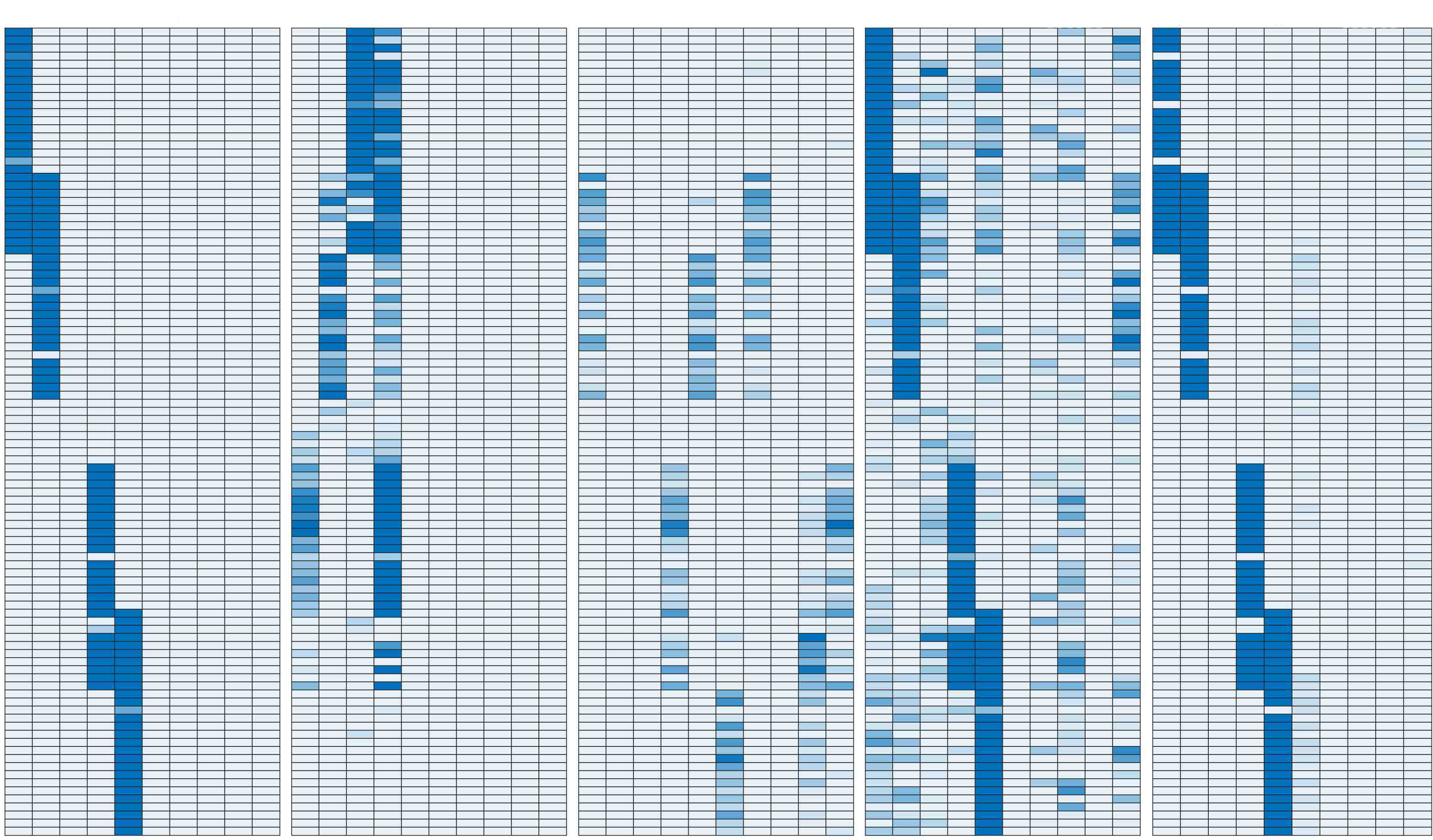
(b) $t=200$

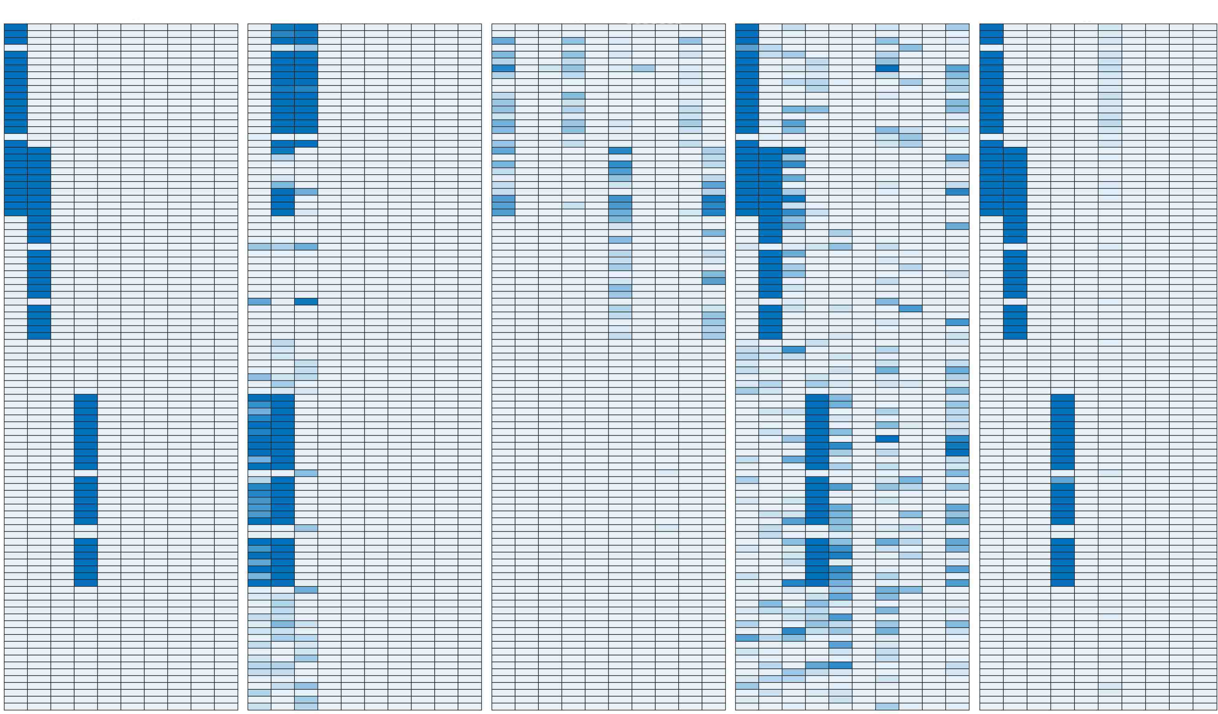
(c) $t=300$

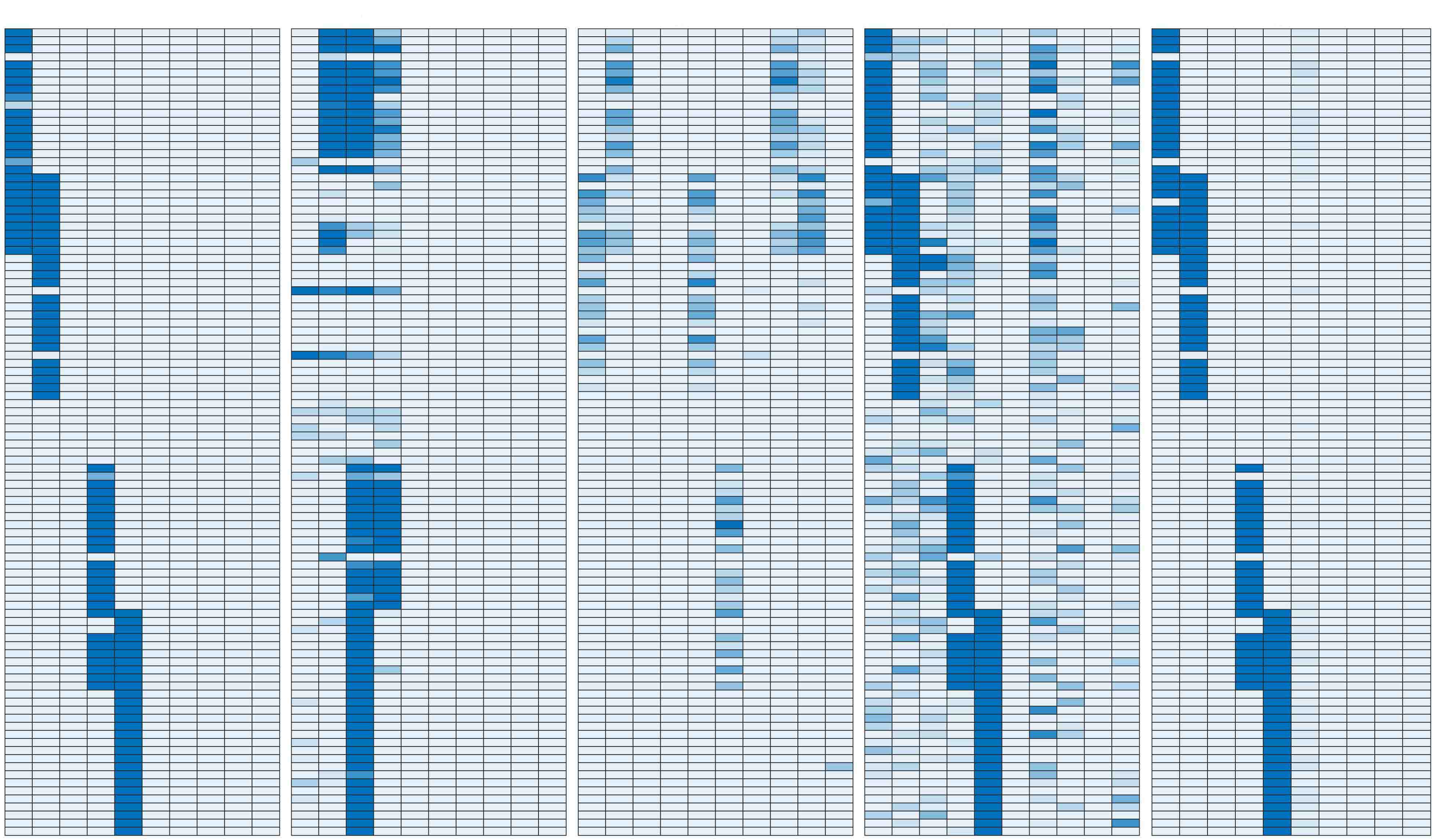
(d) $t=400$

Figure 2: Simulated Example: Heatmaps of true and estimated factor loadings at $t=\{100,200,300,400\}$. Comparisons are made between (from left to right), the true factor loadings, “Adaptive PCA,” “Sparse PCA” ($K=10$), rolling window spike-and-slab factor analysis ($K=10$), and our dynamic spike-and-slab factor analysis. The first three methods are estimated using a rolling window of $100$ data points. Factor loadings are absolute and capped at $0.5$ for visibility.

We compare our proposed dynamic spike-and-slab factor selection with three other approaches. The first one is the “rolling window” version of the static factor analysis with rotations to sparsity by Rockova and George (2016) using $K=10$ (i.e. overshooting the true factor dimensionality). We compare this approach with “Adaptive PCA” of Bai and Ng (2002), which corresponds to a rolling-window principal component analysis (PCA) with estimated number of factors, and with “Sparse PCA” using $K=10$, which is a rolling-window LASSO-based regularization method with cross-validation for selecting the level of shrinkage (Witten et al., 2009). All these methods are estimated using a rolling window of size $100$, where we generate extra $100$ training data points using the sparsity pattern $\boldsymbol{B}^{0}_{1}$. We choose $\widetilde{\phi}=0.95$ and $\sigma^{2}_{\omega}=1-\widetilde{\phi}^{2}$. To deploy the dynamic spike-and-slab priors, we set $\phi_{0}=0$, $\phi_{1}=0.98$, $\lambda_{0}=0.9$, $\lambda_{1}=10(1-\phi_{1}^{2})$, and $\Theta=0.9$ (following the recommendations in Rockova and McAlinn, 2017). To improve the performance of our EM method, we initialize the procedure using the output from the rolling window static spike-and-slab factor model of Rockova and George (2016).

Focusing on the reconstruction of factor loadings, we take snapshots at times $t=\{100,200,300,400\}$ and visually compare the output to the truth (Figure 2). We see that both spike-and-slab methods achieve good recovery. However, the static spike-and-slab cannot fully contain the dynamic loadings, where we see a lot of spillover to other factors. Dynamic spike-and-slab shrinkage, on the other hand, smooths out the sparsity over time, clearly improving on the recovery. “Adaptive PCA” performs well, correctly specifying the number of factors. However, the factor loadings are non-sparse and rotated. “Sparse PCA” with $K=10$ is fairly successful, recovering the blocking structure correctly, but splitting the signal among multiple factors (an observation made also by Rockova and George, 2016). For the spike-and-slab methods, these patterns can be alternatively obtained by thresholding conditional inclusion probabilities rather than just looking at nonzero entries in $\smash{\widehat{\boldsymbol{B}}}_{1:T}$.

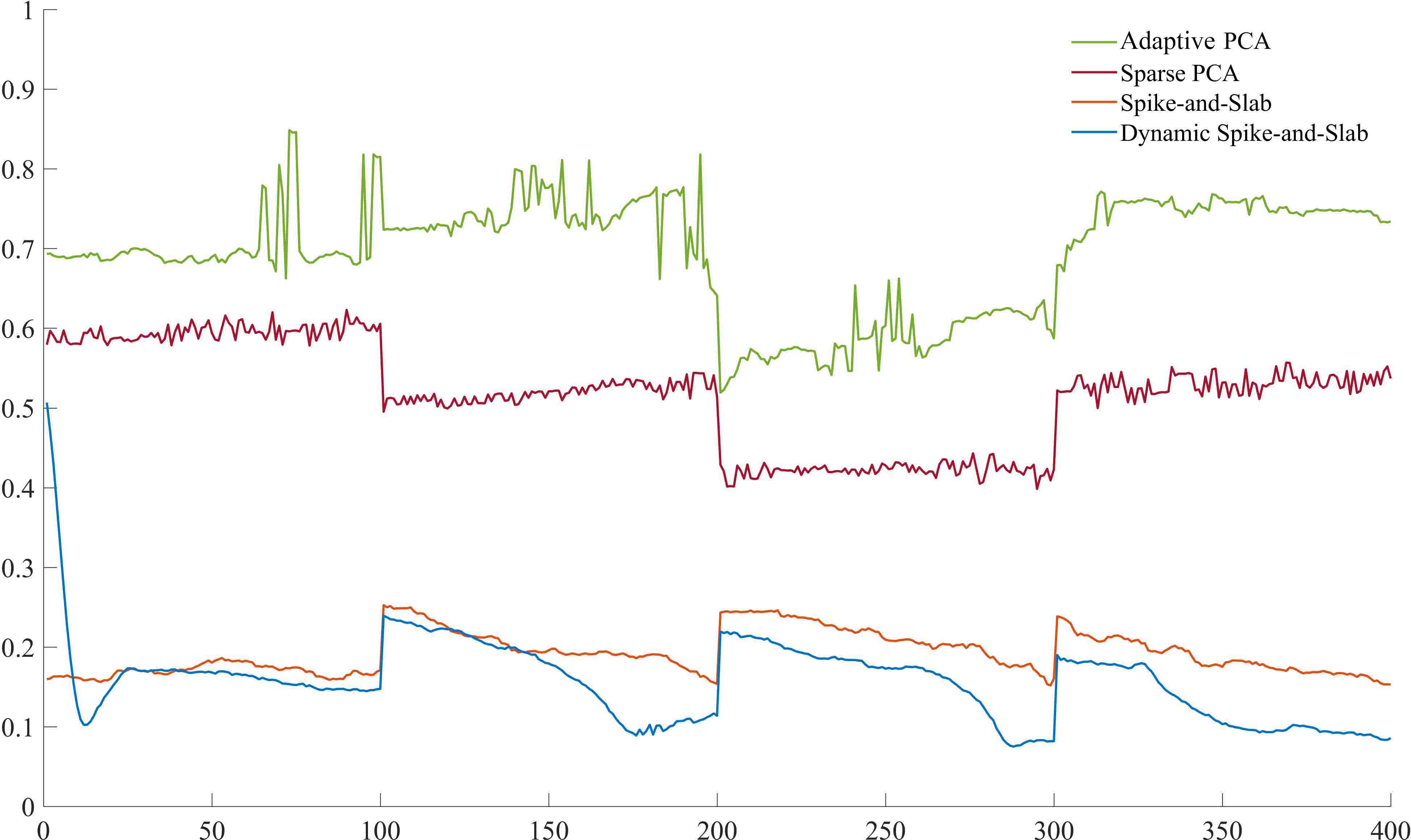
(a) RMSE

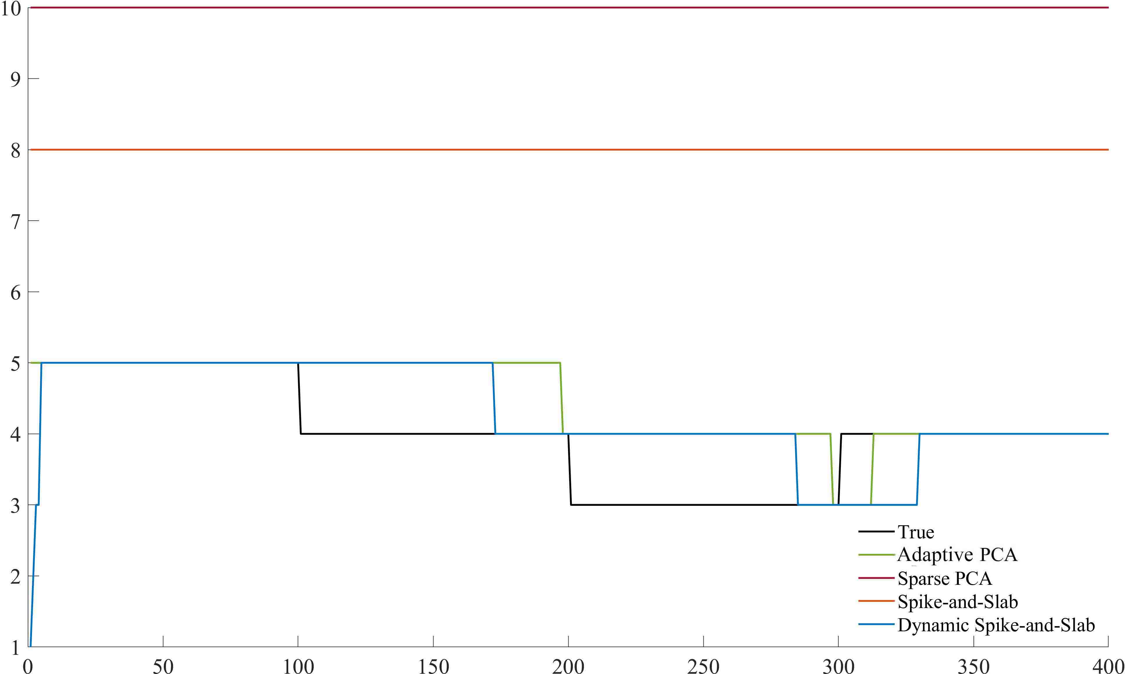
(b) $\smash{\widehat{K}}$

Figure 3: Simulation Study: (Left) The root mean squared error (9) and (Right) the estimated number of factors for “Adaptive PCA,” “Sparse PCA,” static spike-and-slab, and dynamic spike-and-slab, calculated for each $t=1{:}400$.

We further explore how the root mean squared errors (RMSE) change over time for one of the simulations (Figure 3). This is calculated for each $t=1:T$ by

$$RMSE(\smash{\widehat{\boldsymbol{B}}}_{t})=\sqrt{\frac{tr(\boldsymbol{B}^{0}_{t}-\smash{\widehat{\boldsymbol{B}}}_{t})^{\prime}(\boldsymbol{B}^{0}_{t}-\smash{\widehat{\boldsymbol{B}}}_{t})}{P\times K}},$$ (9)

where $\smash{\widehat{\boldsymbol{B}}}_{t}$ are the estimated factor loadings at time $t$. Since this comparison is not entirely meaningful due to the rotational invariance, we compute (9) for the left-ordered variants of these matrices. By looking at the speed of decrease in RMSE after a structural change, it is clear that dynamic spike-and-slab adapts faster compared to its rolling window counterpart. The drop of RMSE for “Adaptive PCA” in periods $101{:}200$ and $201{:}300$ can be attributed to the fact that the number of factors was estimated correctly, resulting in many true zero discoveries. On the other hand, the large estimation error of “Sparse PCA” is due to the lack of sparsity and scattered structure of the factors.

Additionally, we plot the estimated number of factors for each method and compare it to the true number of factors. “Sparse PCA” overestimates the number of factors (where we regard a factor as active if it has at least one nonzero loading). This indicates that unstructured sparsity is not enough. Looking at “Adaptive PCA” and our dynamic spike-and-slab factor model, we find that both perform similarly well in terms of estimating the number of factors. Furthermore, we note that dynamic spike-and-slab adapts faster to factors disappearing, while “Adaptive PCA” adapts faster to factors reappearing.

We repeat the experiment 10 times and report the average RMSE over each of the four stationary interim time periods in Table 2. Dynamic spike-and-slab achieves good recovery, improving upon the rolling window spike-and-slab by as much as 8% to 34% (except for the first period). Large recovery errors of the “Sparse PCA” method can be explained by factor splitting. While “Adaptive PCA” does recover the correct number of factors at each snapshot, the loadings are non-sparse, rotated and non-smooth over time.

	t=1:100			t=101:200			t=201:300			t=301:400
	RMSE	%	$\smash{\widehat{K}}$	RMSE	%	$\smash{\widehat{K}}$	RMSE	%	$\smash{\widehat{K}}$	RMSE	%	$\smash{\widehat{K}}$
Adaptive PCA	1.0660	-266.07	5	1.0590	-400.24	4.97	0.9730	-250.38	3.97	1.033	-430.01	3.88
Sparse PCA	0.7862	-169.99	10	0.7260	-242.94	10	0.6377	-129.64	10	0.7383	-278.81	10
Spike-and-Slab	0.1919	34.10	8	0.2843	-34.29	8	0.2988	-7.60	8	0.2447	-25.60	8
Dynamic Spike-and-Slab	0.2912	-	4.89	0.2117	-	4.72	0.2777	-	3.84	0.1949	-	3.71

Table 2: Simulation Study: Performance evaluation of the latent factor methods compared to the true coefficients for $t=1{:}400$. Performance is evaluated based on RMSE within each evaluation period. % is the performance gain compared to dynamic spike-and-slab. $\smash{\widehat{K}}$ is the average number of factors estimated during that period.

5 Empirical Study

The empirical application concerns a large-scale monthly U.S. macroeconomic database, comprising a balanced panel of $P=127$ monthly macroeconomic and financial variables tracked over the period of $2001/01$ to $2015/12$ ($T=180$). These variables are classified into eight main categories, depending on their economic meaning: Output and Income, Labor Market, Consumption and Orders, Orders and Inventories, Money and Credit, Interest Rate and Exchange Rates, Prices, and Stock Market. A detailed description of how variables were collected and constructed is provided in McCracken and Ng (2016). A quick table of names and groups of each variable is in the Appendix (Table B1). The variables were centered to have mean zero and standardized following the procedures in McCracken and Ng (2016).

The purpose of conducting a sparse latent factor analysis on a large-scale economic dataset, such as this one, is at least twofold. Due to the group structure of the data, it is natural to assume that the measured indicators are tied via a few latent factors, the basic premise of latent factor modeling. Moreover, we expect the sparse latent structure to pickup clusters of dependence structures that capture the interconnectivity of indicators spanning many different aspects of the economy. Sparsity will help extract such interpretable structures. Second, given the dynamic nature of the economy, there is a substantial interest in understanding how these dependencies change over time and– in particular– how they are affected by shocks. We anticipate non-negligible shifts in the economy, as the data spans over the housing bubble deflation after 2006 and the great financial crisis in late 2008, which led to the Great Recession. Understanding the interplay between contributing factors to the financial crisis has been a subject of rigorous research (see for example, Commission, 2011; Reinhart and Rogoff, 2008; Mian and Sufi, 2009, 2011; Mian et al., 2013; Chodorow-Reich, 2014; Benmelech et al., 2017). Our analysis is purely data-driven and thereby descriptive rather than causally conclusive. We attempt to characterize patterns of shock proliferation and permanence of structural changes of the economy using our dynamic factor model.

As the dataset is considerably richer than our simulated example, we expand the model (1) by incorporating a dynamic intercept to capture location shifts that could not be easily standardized away. The intercepts $c_{jt}$ follow independent random walk evolutions with an initial condition $c_{0}\sim N(0,1)$. The initial condition for the SV variances is $1/\sigma_{j0}^{2}\stackrel{{\scriptstyle ind}}{{\sim}}G(n_{0}/2,d_{0}/2)$ for $1\leq j\leq P$ with $n_{0}=20$ and $d_{0}=0.002$. The discount factor is set to 0.95.

(a) “Adaptive PCA”

(b) ”Sparse PCA”

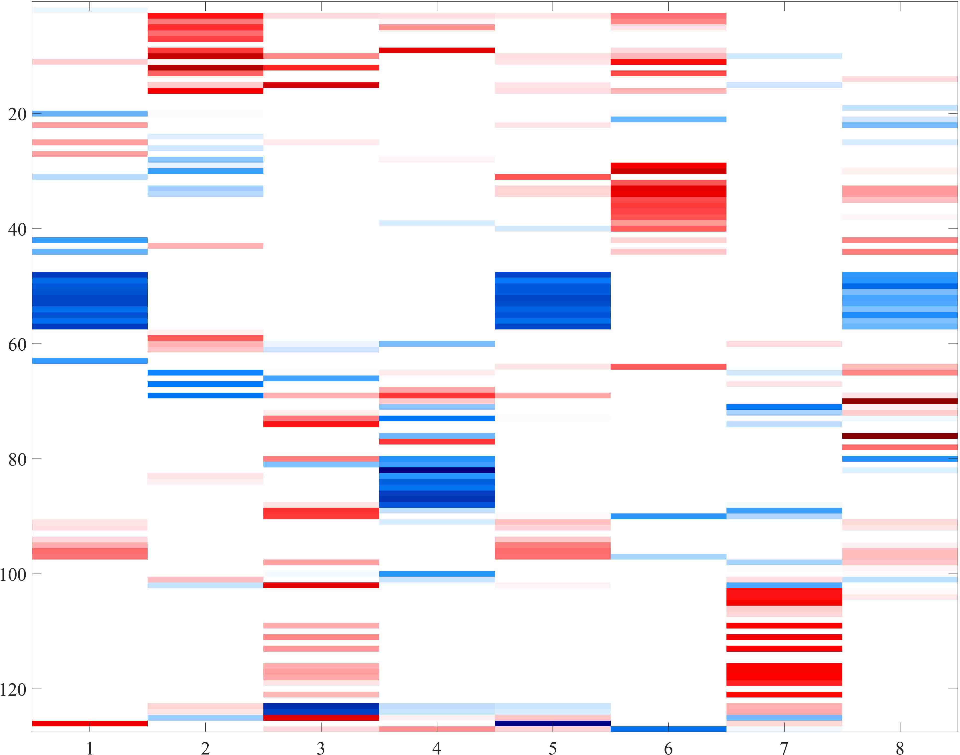
(c) ”Sparse PCA”

Figure 4: Macroeconomic Study: Estimated factor loadings using “Adaptive PCA” (Left), “Sparse PCA” with number of factors set as 30 (Middle), and “Sparse PCA” with number of factors set to 8 from the results of “Adaptive PCA” (Right) at $t=2015/12$, with the number of series on the y-axis and the number of factors in the x-axis. The factor loading are estimated using a $10$ year rolling window.

First, we examine one snapshot of the output from “Adaptive PCA” and “Sparse PCA” (described in Section 4) at time $2015/12$ (Figures 4). Both methods do pick up certain groupings, but do not yield interpretable enough representations. This is likely due to overestimation of the number of factors (Figure 4 (b)), factor rotation and lack of sparsity (Figure 4 (a)) and/or factor splitting (Figure 4 (c)). Next, we deploy the rolling window spike-and-slab factor method with a training period of 10 years to obtain starting values for our dynamic factor model. Priors and their hyper-parameters were chosen as in the simulation study. We choose a generous upper bound $K=126$ on the number of factors, letting the sparsity rule out factors that are irrelevant.

We now examine the output of our procedure at three time points: 2003/12, 2008/10, and 2015/12. These three snapshots are of particular interest as they represent three distinct states of the economy: relative stability (2003), sharp economic crisis (2008), and recovery (2015). 2008/10 is at the onset of the great financial crisis, where deflation of the housing bubble after 2006 lead to mortgage delinquencies and financial fragility (Commission, 2011). This distress permeated throughout the rest of the economy, including the labor market, leading to the deepest recession in post-war history.

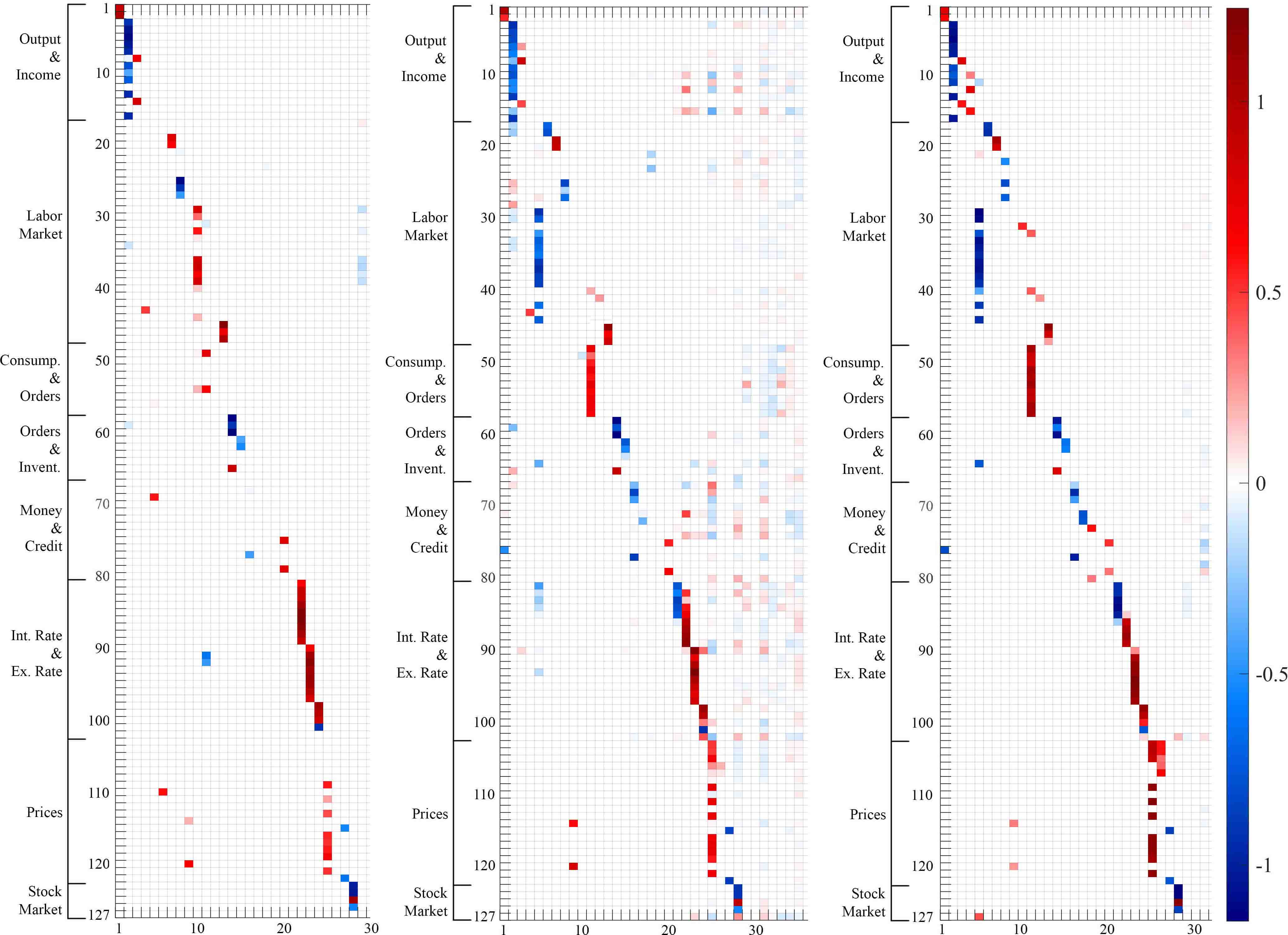
Figure 5: Macroeconomic Study: Estimated factor loadings using dynamic sparse factor analysis at $t=2003/12$ (left), $t=2008/10$ (center), $t=2015/12$ (right), with the original series on the y-axis and the factors in the x-axis. The factor loading are estimated dynamically over the period $2001/1{:}2015/12$.

The heatmap of estimated factor loadings at time $2003/12$ is in Figure 5 (left). The output has been left-ordered based on the results at $2015/12$, where the more active factors are on the left, in the order of data series, and some of the less active right-most factors (with small or zero loadings) are omitted. There are $24$ active factors in total (i.e. factors with at least two non-negligible non-zero factor loadings), with only $5$ factors that cluster eight or more series (Factors 2, 10, 22, 23, and 25). Since the variables are grouped by their economic meaning, this type of clustering is not entirely unexpected. For example, Factor 2 includes CMRMTSPLx (real manufacturing and trade industry sales), all industrial production indices except nondurable materials, residential utilities, and fuels, CUMFNS (capacity utilization), DMANEMP (durable goods employment), and ISRATIOx (manufacturing and trade inventories to sales ratio). This factor could be interpreted as a factor for durable goods, which include industries that are more susceptible to economic trends, where sales, inventories, industrial production, capacity utilization, and employment are all connected. Conversely, we expect nondurable goods, such as utilities and fuels, to have a different dynamic than durable goods, which is reflected in the exclusion of those indices in Factor 2. Similarly, Factor 10 includes employment data (except for mining and logging, manufacturing, durable goods, nondurable goods, and government), Factor 22 includes interests rates (fed funds rate, treasury bills, and bond yields), Factor 23 includes the spread between interest rates minus fed funds rate, and Factor 25 includes consumer price indices except apparel, medical care, durables, and services, as well as personal consumptions expenditures on nondurable goods. All of these factors produce meaningful and mostly separated clusters that largely conform with economic intuition.

During the crisis (Figures 5; center), radical changes occur in the factor structure. Concerning Factor 2, the dependence structure expands, now spanning over nondurables and fuels, as well as HWI (the help wanted index), UNEMP15OV (unemployment for 15 weeks and over), CLAIMSx (unemployment insurance claims), and PAYEMS (employment, total non-farm, goods-producing, manufacturing, and durable goods). This indicates that the shock might have affected relatively stable industries and unemployment, with the co-movement across industries being largely synchronized under distress (with the exception of residential utilities). Another interesting observation is the emergence of new factors. In particular, Factor 11, which includes housing starts and new housing permits in different regions in the U.S., was not present pre-crisis and now surfaces as a connecting thread between housing markets across regions. While in $2003/12$ the latent factors were largely separated (loadings had little overlap), we now see at least two factors (namely Factor 25 and 28), whose loadings are non-sparse and far-reaching. In particular, Factor 28 emerges as a non-sparse link between many different sectors of the economy, including retail sales, industrial production, employment (in particular financial services), real M2 money stock, loans, BAA bond yields (but not AAA), exchange rates, consumer sentiment, investment and, most importantly, the stock market indices, including the S&P 500 and the VIX (i.e. the fear index). Factor 25, on the other hand, is driven mainly by prices (e.g. CPI). Both of these factors could be potentially interpreted as crisis factors as they are connected to the various corners of the economy, except Consumption and Orders; the housing market. The “orthogonality” between the housing market factor (Factor 11) and the “crisis factors” (Factor 25 and 28) may suggest that, while the crisis was triggered by the housing market, the main catalyst of the recession was the financial market. While our analysis does not necessarily prove this hypothesis, it aligns with previous lines of reasoning. In particular, there have been arguments that the devaluation of securities, including mortgage backed securities, ultimately led to curtailed lending and decreased investment and consumption (Chodorow-Reich, 2014; Benmelech et al., 2017).

Finally, Figure 5 (right) shows the end of the analysis at $2015/12$, where the economy has mostly recovered from the Great Recession, but has fundamentally changed from what it was before. Although most of the factor overlap has dissipated, we see a notably different structure compared to 2003. In particular, Factor 5 (employment) and Factor 11 (housing) persevere from the crisis. Moreover, the “crisis factors” Factor 25 and 28, representing the prices and the stock market, are no longer strongly tied to other parts of the economy (labor, output, interest and exchange rates, etc.). Factor 2 is one of the few factors that have returned back to its original structure, except for CMRMTSPLx and industrial production of nondurable consumer goods. Its dependence with the labor market (e.g. unemployment) has disappeared, suggesting that industry production is no longer in co-movement with the labor market.

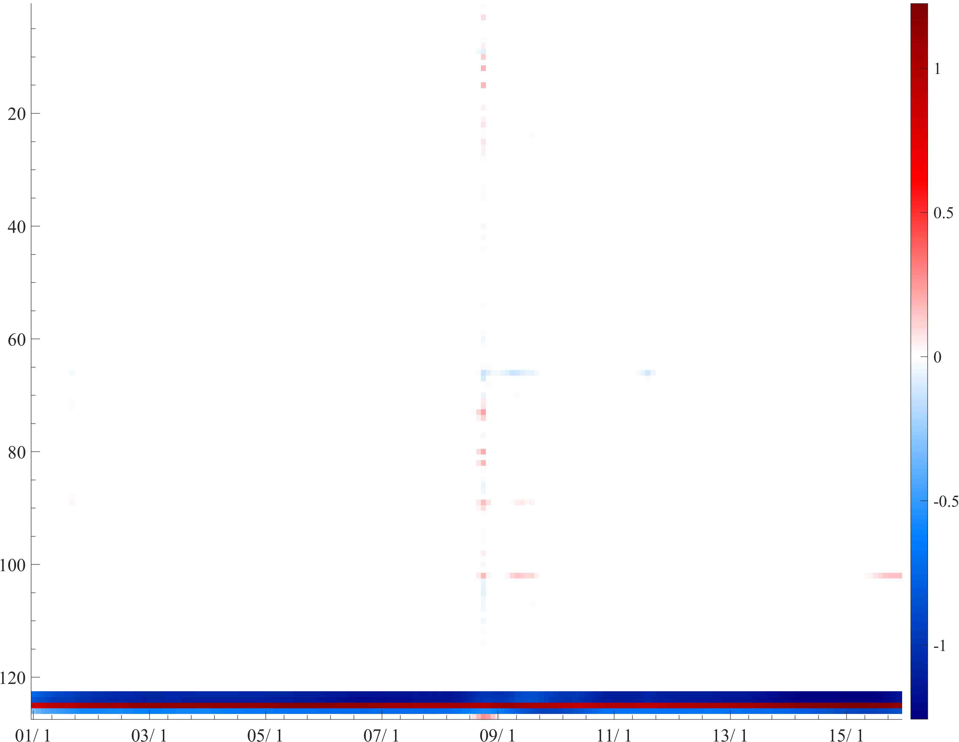
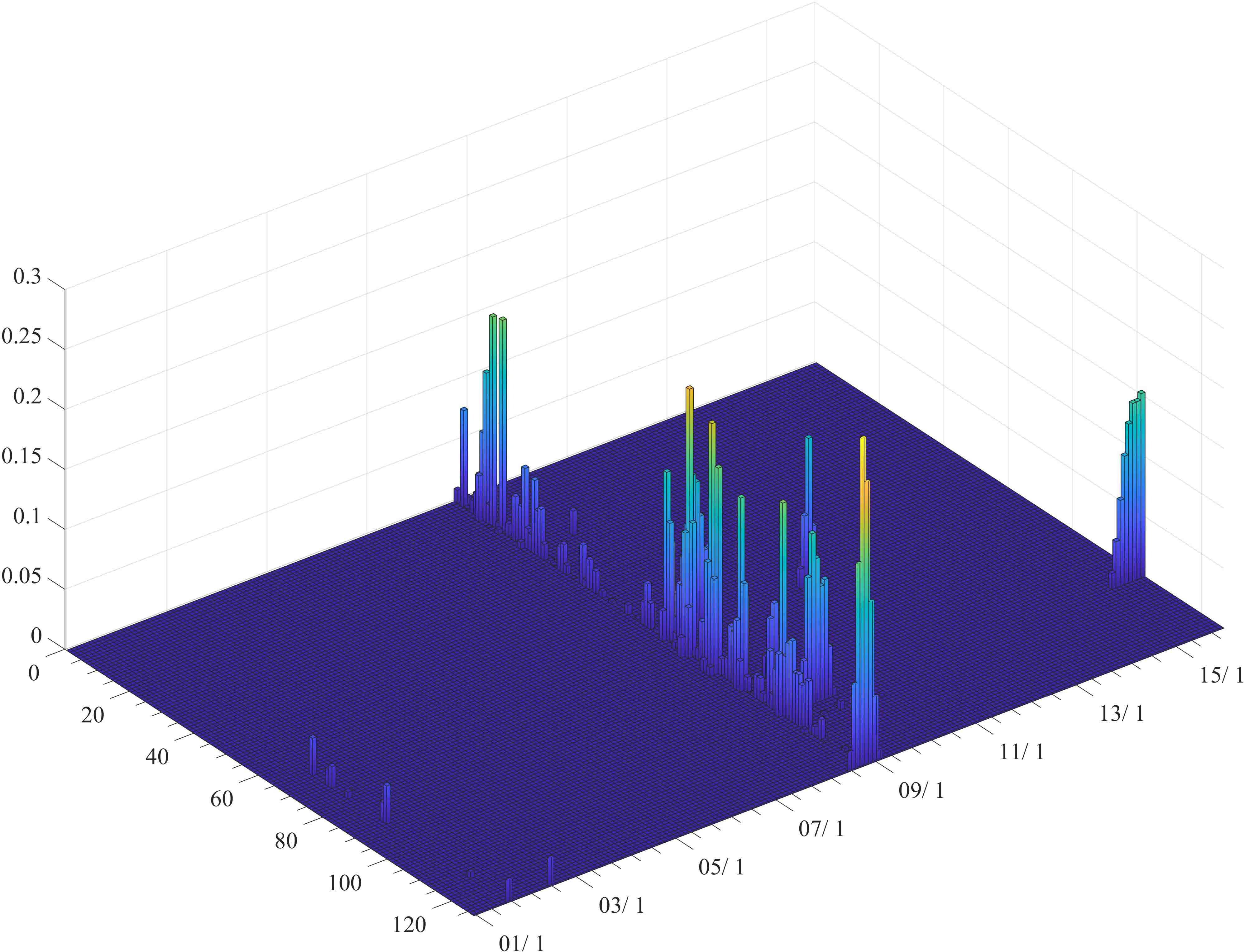
Figure 6: Macroeconomic Study: Estimated factor loadings for Factor 28 using dynamic spike-and-slab from $t=200/12{:}2015/12$, with a heatmap of the entire factor loadings (Left) and a 3-D plot of the factor loadings with the loadings on 123-126 (S&P related indices) set to zero to increase visibility.

We also obtain insights into the effects and duration of the crisis by looking at the evolution of the factor loadings for one of the “crisis” factors, Factor 28. Figure 6 shows a dynamic heatmap and a $3$-D plot of $\beta_{jk}^{t}$ for $1\leq j\leq 127$ (y-axis) and $1\leq t\leq 180$ (x-axis) with $k=28$. For the $3$-D plot, the loadings on the S&P indices are suppressed to zero in order to improve visibility. The figure reveals a spur of activity around the sharp financial crisis (late 2008 and early 2009), where the contagion battered multiple corners of the economy. The duration of the active loadings provide additional insights. For example, the loadings on VIX (series 127) emerges and disappears in a eight month span from 06/2008 to 02/2009, while the loadings on the exchange rate between U.S. and Canada lasts for $17$ months. However, most factor loadings seem to only emerge for about 4-6 months.

To understand the degree of connectivity/overlap between factors, we plot the average number of active factors per series over time (Figure 7). More overlap indicates a more intertwined economy. We observe an increase in late $2008$, reflecting the emergence pervasive crisis factor(s), as well as its build up from mid-2006. Another point to note is that the level pre-crisis is comparatively lower than post-crisis, indicating a structural shift is the economy brought on by the crisis.

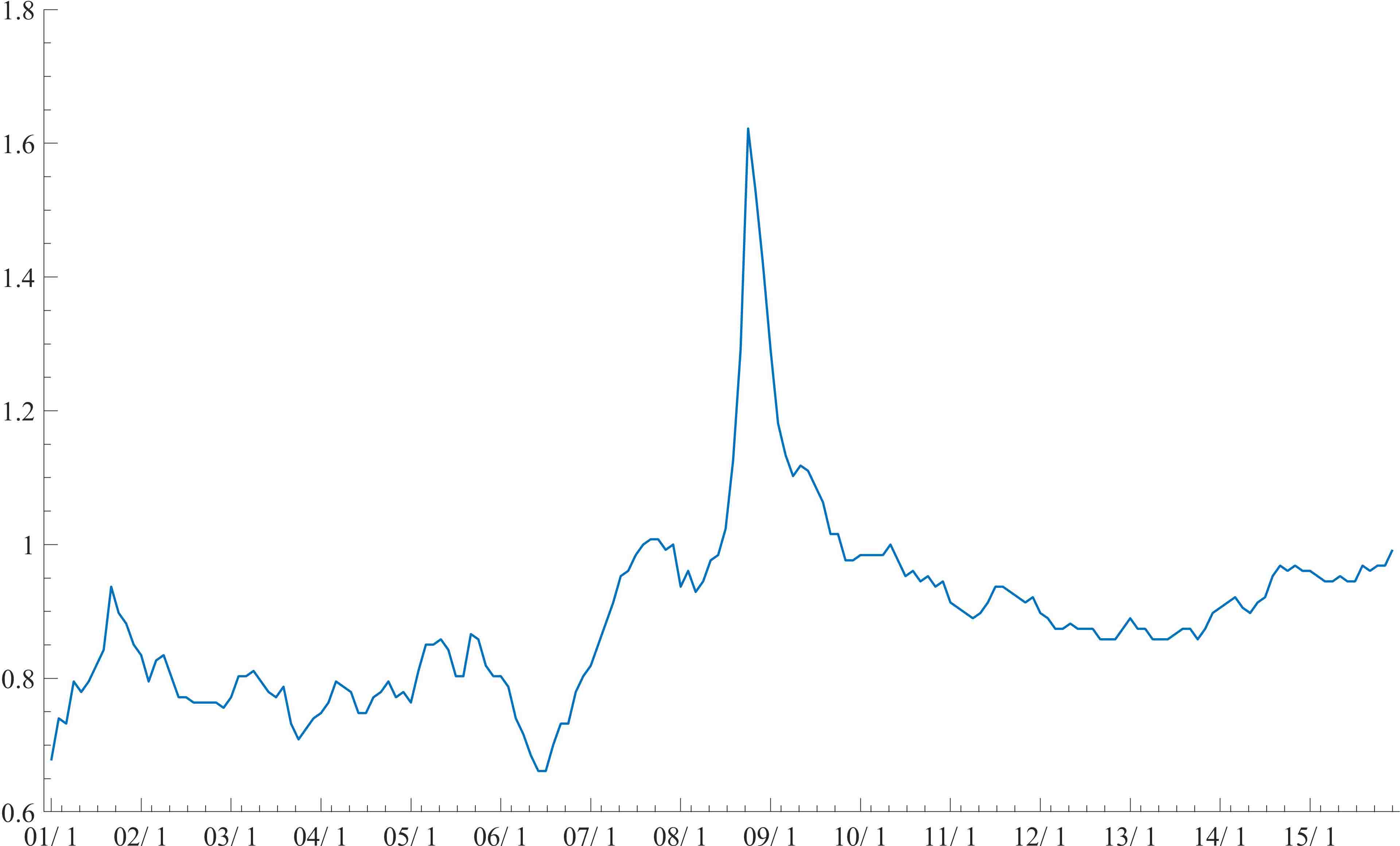
Figure 7: Macroeconomic Study: The average number of estimated active factors (with absolute loadings above $0.1$) per series over the period $2001/1{:}2015/12$.

We further our analysis with a few insights into the idiosyncratic variances for variables related to the housing market: HOUST (total housing starts) and its regional variants (North East, Mid-West, South, and West). Housing starts is the seasonally adjusted number of new residential construction projects that have begun during any particular month and, as such, is a key part of the U.S. economy, which relates to employment and many industry sectors including banking (the mortgage sector), raw materials production, construction, manufacturing, and real estate. In our earlier analysis (Figure 5) we found that, while regional indicators were not clustered pre-crisis, persistent clustering occurs post-crisis. Figure 8 portrays the series of residual uncertainties $\{\sigma^{2}_{jt}:1\leq t\leq T\}$ for each regional housing starts indicator. We find several interesting patterns. Figure 8 indicates that increased uncertainty in housing starts is a global phenomenon but that there is heterogeneity across regions as to the magnitude and timing. For example, we find that the West region to react the earliest, followed by Mid-West and South. North-East is somewhat of an exception, as the idiosyncratic variance starts out greater than the other series, falling off pre-crisis, increasing during the crisis, and tapering off to a level similar to the other regions. The speed of mounting uncertainty could be associated with the deflation of the housing bubble after 2006 (Commission, 2011). As the economy recovers from the Great Recession, we observe a gradual decrease in uncertainty, where different regions recover at different paces.

Figure 8: Macroeconomic Study: The idiosyncratic variance, $\mbox{\boldmath$\Sigma$}_{t}$, of U.S. housing starts, over the period $2001/1{:}2015/12$.

6 Further Comments

Motivated by a topical macroeconomic dataset, we developed a Bayesian method for dynamic sparse factor analysis for large-scale time series data. Our proposed methodology aims to tackle three challenges of dynamic factor analysis: time-varying patterns of sparsity, unknown number of factors, and identifiability constraints. By deploying dynamic sparsity, we successfully recover interpretable latent structures that automatically select the number of factors and that incorporate time-varying loadings/factors. We successfully applied our methodology on a nontrivial simulated example as well as a real dataset comprising of 127 U.S. macroeconomic indices tracked over the period of the Great Recession (and beyond) and obtained several interpretable findings.

Our methodology can be enriched/extended in many ways. One possible extension would be to develop a latent variable method that can capture within, as well as between, connectivity of several high-dimensional time series. This could be achieved with a dynamic extension of sparse canonical correlation analysis (Witten et al., 2009). Our method can also be embedded within FAVAR models (Bernanke et al., 2005) that include both observed and unobserved predictors. Additionally, throughout our analysis we have assumed the covariance of the latent factors to be fixed over time and equal to an identity matrix, one could in principle incorporate dynamic variances with stochastic volatility modeling.

One possible shortcoming of our proposed methodology, which is shared by all EM based estimation strategies, is the lack of uncertainty assessment, which is essential for forecasting. The EM algorithm, however, was the key to obtaining interpretable latent structures. To achieve both, one could impose identification constraints, such as Nakajima and West (2013b, a), and perform MCMC for DSS priors along the lines of Rockova and McAlinn (2017). Another approach would be to apply our method simply as a means of obtaining identifiability constraints (i.e. the sparsity pattern) and then reestimate the nonzero loadings with an MCMC strategy. While this would not quantify any sparsity-selection uncertainty, it would be an effective way to balance interpretability and forecasting/decision making. Another unavoidable feature of our method is its sensitivity to starting values. We strongly recommend using the output from the rolling window spike-and-slab factor model.

Appendix A Appendix

A.1 Derivation of the E-step

We now outline the steps of the parameter expanded EM algorithm. In the E-step, we compute the conditional expectation of the augmented and expanded log-posterior with respect to the missing data $\boldsymbol{\Omega}$ and $\boldsymbol{\Gamma}$, given observed data $\boldsymbol{Y}$ and the parameter values $\boldsymbol{\Delta}^{(m)}$ obtained at the previous M-step setting $\mbox{\boldmath$A$}_{t}=\sigma^{2}_{\omega}\boldsymbol{I}_{K}$. We can write

$$\mathbb{E}_{\boldsymbol{\Gamma},\boldsymbol{\Omega}\,|\>\boldsymbol{Y},\Delta^{(m)}}[\log\pi(\boldsymbol{B}^{\star}_{0:T},\mbox{\boldmath$\Sigma$}_{1:T},\mbox{\boldmath$A$}_{1:T},\boldsymbol{\Gamma},\boldsymbol{\Omega}\,|\>\boldsymbol{Y})]= Q_{1}(\boldsymbol{B}_{0:T}^{\star}\,|\>\mbox{\boldmath$\Sigma$}_{1:T})+Q_{2}(\mbox{\boldmath$\Sigma$}_{1:T})+Q_{3}(\mbox{\boldmath$A$}_{1:T})+C.$$ (10)

Define $\boldsymbol{\omega}_{t|T}=\mathbb{E}_{\boldsymbol{\Omega}}[\boldsymbol{\omega}_{t}\,|\>\boldsymbol{Y},\boldsymbol{\Delta}^{(m)}]$, $\mbox{\boldmath$V$}_{t|T}=\mathrm{cov}[\boldsymbol{\omega}_{t}\,|\>\boldsymbol{Y},\boldsymbol{\Delta}^{(m)}]$. The terms $\boldsymbol{\omega}_{t|T}$ and $\mbox{\boldmath$V$}_{t|T}$ represent the best linear estimator for $\boldsymbol{\omega}_{t}$ using all observations and the corresponding covariance matrix, respectively. With $\mbox{\boldmath$V$}_{t,t-1|T}=\mathrm{cov}[\boldsymbol{\omega}_{t},\boldsymbol{\omega}_{t-1}\,|\>\boldsymbol{Y},\boldsymbol{\Delta}^{(m)}]$ we denote the covariance matrix of $\boldsymbol{\omega}_{t}$ and $\boldsymbol{\omega}_{t-1}$ given the data $\boldsymbol{Y}$ and $\boldsymbol{\Delta}^{(m)}$. These quantities can be obtained from the Kalman Filter and Smoother Algorithm (Table 3).

The functions $Q_{1}(\cdot)$, $Q_{2}(\cdot)$ and $Q_{3}(\cdot)$ in (10) can be written as follows:

$$-Q_{1}(\boldsymbol{B}_{0:T}^{\star}\,|\>\mbox{\boldmath$\Sigma$}_{1:T})= C+\frac{1}{2}\sum_{t=1}^{T}\sum_{j=1}^{P}\log\sigma_{jt}^{2}$$

$$+tr\left\{\frac{1}{2}\sum_{t=1}^{T}\boldsymbol{\Sigma}_{t}^{-1}\left[(\boldsymbol{Y}_{t}-\boldsymbol{B}_{t}^{\star}\boldsymbol{\omega}_{t|T})(\boldsymbol{Y}_{t}-\boldsymbol{B}_{t}^{\star}\boldsymbol{\omega}_{t|T})^{\prime}+\boldsymbol{B}_{t}^{\star}\mbox{\boldmath$V$}_{t|T}\boldsymbol{B}^{\star^{\prime}}_{t}\right]\right\}$$

$$+\sum_{j=1}^{P}\sum_{k=1}^{K}\left[\frac{\langle\gamma_{jk}^{0}\rangle(\beta_{jk}^{0*})^{2}}{2\lambda_{1}/(1-\phi^{2})}+(1-\langle\gamma_{jk}^{0}\rangle)|\beta_{jk}^{0*}|\lambda_{0}\right]$$

$$+\sum_{t=1}^{T}\sum_{j=1}^{P}\sum_{k=1}^{K}\left[\frac{\langle\gamma_{jk}^{t}\rangle(\beta_{jk}^{t*}-\phi\beta_{jk}^{t-1*})^{2}}{2\lambda_{1}}+(1-\langle\gamma_{jk}^{t}\rangle)|\beta_{jk}^{t*}|\lambda_{0}\right],$$

where

$$\langle\gamma_{jk}^{0}\rangle =\frac{\Theta\psi_{1}(\beta_{jk}^{0}|0,\frac{\lambda_{1}}{1-\phi^{2}})}{\Theta\psi_{1}(\beta_{jk}^{0}|0,\frac{\lambda_{1}}{1-\phi^{2}})+(1-\Theta)\psi_{0}(\beta_{jk}^{0}|0,\lambda_{0})},$$

$$\langle\gamma_{jk}^{t}\rangle =\frac{\theta_{jk}^{t}\psi_{1}(\beta_{jk}^{t}|\phi\beta_{jk}^{t-1},\lambda_{1})}{\theta_{jk}^{t}\psi_{1}(\beta_{jk}^{t}|\phi\beta_{jk}^{t-1},\lambda_{1})+(1-\theta_{jk}^{t})\psi_{0}(\beta_{jk}^{t}|0,\lambda_{0})},$$

$$-Q_{2}(\mbox{\boldmath$\Sigma$}_{1:T}) =\sum_{t=1}^{T-1}\sum_{j=1}^{P}\left[pen(\sigma_{jt}^{2}\,|\>\sigma_{j(t-1)}^{2})+pen(\sigma_{jt}^{2}\,|\>\sigma_{j(t+1)}^{2})\right]+\sum_{j=1}^{P}pen(\sigma_{jT}^{2}\,|\>\sigma_{j(T-1)}^{2})$$

where

$$pen(\sigma_{jt}^{2}\,|\>\sigma_{j(t-1)}^{2}) =\left(\frac{\delta n_{t-1}}{2}-1\right)\log{\sigma_{jt}^{2}}-\left(\frac{(1-\delta)n_{t-1}}{2}-1\right)\log{\left(1-\frac{\delta\sigma_{j(t-1)}^{2}}{\sigma_{jt}^{2}}\right)},$$

$$pen(\sigma_{jt}^{2}\,|\>\sigma_{j(t+1)}^{2}) =-\left(\frac{\delta n_{t}}{2}-1\right)\log{\sigma_{jt}^{2}}+\left(\frac{(1-\delta)n_{t}}{2}-1\right)\log{\left(1-\frac{\delta\sigma_{jt}^{2}}{\sigma_{j(t+1)}^{2}}\right)},$$

and

Algorithm: Kalman Filter and Smoother
Initialize $\boldsymbol{\omega}_{0\,|\>0}=\boldsymbol{0}$ and $\mbox{\boldmath$V$}_{0\,|\>0}=\sigma^{2}_{\omega}/(1-\widetilde{\phi}^{2})\boldsymbol{I}_{K}$
Repeat the Prediction Step and Correction Step for $t=1,\dots,T$
Prediction Step	$\boldsymbol{\omega}_{t\,|\>t-1}=\boldsymbol{\omega}_{t-1\,|\>t-1}$
	$\mbox{\boldmath$V$}_{t\,|\>t-1}=\mbox{\boldmath$V$}_{t-1\,|\>t-1}+\sigma^{2}_{\omega}\boldsymbol{I}_{K}$
Correction Step	$\boldsymbol{K}_{t}=\mbox{\boldmath$V$}_{t\,|\>t-1}\boldsymbol{B}_{t}^{\prime}(\boldsymbol{B}_{t}\mbox{\boldmath$V$}_{t\,|\>t-1}\boldsymbol{B}_{t}^{\prime}+\mbox{\boldmath$\Sigma$}_{t})^{-1}$
	$\boldsymbol{\omega}_{t\,|\>t}=\boldsymbol{\omega}_{t\,|\>t-1}+\boldsymbol{K}_{t}(\boldsymbol{Y}_{t}-\boldsymbol{B}_{t}\boldsymbol{\omega}_{t\,|\>t-1})$
	$\mbox{\boldmath$V$}_{t\,|\>t}=\mbox{\boldmath$V$}_{t\,|\>t-1}-\boldsymbol{K}_{t}\boldsymbol{B}_{t}\mbox{\boldmath$V$}_{t\,|\>t-1}$
Initialize $\mbox{\boldmath$V$}_{T,T-1\,|\>T}=(I-\boldsymbol{K}_{T}\boldsymbol{B}_{T})\mbox{\boldmath$V$}_{T-1\,|\>T-1}$
Repeat the smoothing step for $t=T,\dots,1$
Smoothing Step	$\boldsymbol{\omega}_{t-1\,|\>T}=\boldsymbol{\omega}_{t-1\,|\>t-1}+\boldsymbol{Z}_{t-1}(\boldsymbol{\omega}_{t\,|\>T}-\boldsymbol{\omega}_{t\,|\>t-1})$
	$\mbox{\boldmath$V$}_{t-1\,|\>T}=\mbox{\boldmath$V$}_{t-1\,|\>t-1}+\boldsymbol{Z}_{t-1}(\mbox{\boldmath$V$}_{t\,|\>T}-\mbox{\boldmath$V$}_{t\,|\>t-1})\boldsymbol{Z}_{t-1}^{\prime}$
	$\mbox{\boldmath$V$}_{t,t-1\,|\>T}=\mbox{\boldmath$V$}_{t-1\,|\>t-1}\boldsymbol{Z}_{t-2}^{\prime}+\boldsymbol{Z}_{t-1}(\mbox{\boldmath$V$}_{t,t-1\,|\>T}-\mbox{\boldmath$V$}_{t-1\,|\>t-1})\boldsymbol{Z}_{t-2}^{\prime}$
	where $\boldsymbol{Z}_{t-1}=\mbox{\boldmath$V$}_{t-1\,|\>t-1}\mbox{\boldmath$V$}_{t\,|\>t-1}^{-1}$

Table 3: Kalman Filter and Smoother Algorithm for Parameter Expanded EM using rotated loading matrices $\boldsymbol{B}_{1:T}$

$$-Q_{3}(\mbox{\boldmath$A$}_{1:T}) =\frac{1}{2}\sum_{t=1}^{T}\log|\mbox{\boldmath$A$}_{t}|+\frac{1}{2}tr\{\mbox{\boldmath$A$}_{t}^{-1}(\boldsymbol{M}_{1t}-\boldsymbol{M}_{12t}-\boldsymbol{M}_{12t}^{\prime}+\boldsymbol{M}_{2t})\},$$

where

$$\boldsymbol{M}_{1t} =(\boldsymbol{\omega}_{t-1\,|\>T}\boldsymbol{\omega}_{t-1\,|\>T}^{\prime}+\mbox{\boldmath$V$}_{t-1\,|\>T}),$$

$$\boldsymbol{M}_{12t} =(\boldsymbol{\omega}_{t-1\,|\>T}\boldsymbol{\omega}_{t\,|\>T}^{\prime}+\mbox{\boldmath$V$}_{t,t-1\,|\>T}),$$

$$\boldsymbol{M}_{2t} =(\boldsymbol{\omega}_{t\,|\>T}\boldsymbol{\omega}_{t\,|\>T}^{\prime}+\mbox{\boldmath$V$}_{t\,|\>T}).$$

A.2 Derivation of the M-step

In the M-step, we optimize the function $Q_{1}(\cdot)$ with respect to $\boldsymbol{B}_{0:T}^{\star}$, given values of $\mbox{\boldmath$\Sigma$}_{1:T}$ from the previous M-step. Given the new values $\boldsymbol{B}_{0:T}^{\star(m+1)}$ and the posterior moment estimates of the latent factors obtained from the Kalman filter, we optimize $Q_{1}(\cdot)+Q_{2}(\cdot)$, with respect to $\mbox{\boldmath$\Sigma$}_{1:T}$. Finally, we optimize the function $Q_{3}(\cdot)$ with respect to $\mbox{\boldmath$A$}_{1:T}$.

Optimizing $Q_{1}(\cdot)$ with respect to $\boldsymbol{B}^{\star}_{0:T}$ boils down to solving a series of independent dynamic spike and slab LASSO regressions (similarly as in(Rockova and McAlinn, 2017)). This is justified by the following lemma.

Lemma A.1.

Let $\boldsymbol{Y}^{t}=(Y^{t}_{1},\dots,Y^{t}_{P})^{\prime}\in\mathbb{R}^{P}$ denote the snapshot of the series at time $t$ and for $1\leq j\leq P$ define a zero-augmented response vector at time $t$ with $\widetilde{\boldsymbol{Y}}^{t}_{j}=(Y^{t}_{j},\underbrace{0,\dots,0}_{K})^{\prime}\in\mathbb{R}^{K+1}$. For the SVD decomposition $\mbox{\boldmath$V$}_{t\,|\>T}=\sum_{k=1}^{K}s_{k}\boldsymbol{U}_{k}^{t}(\boldsymbol{U}_{k}^{t})^{\prime}$, we denote with $\widetilde{\boldsymbol{U}}_{k}^{t}=\sqrt{s_{k}}\boldsymbol{U}_{k}^{t}$ and with $\boldsymbol{\Omega}^{t}=[\boldsymbol{\omega}_{t|T},\widetilde{\boldsymbol{U}}_{1}^{t},\dots,\widetilde{\boldsymbol{U}}_{K}^{t}]^{\prime}\in\mathbb{R}^{(1+K)\times K}$ and we let $\boldsymbol{\beta}^{t\star^{\prime}}_{j}\in\mathbb{R}^{K}$ be the $j^{th}$ row of $\boldsymbol{B}_{t}^{\star}$. Then we can decompose

$$Q_{1}(\boldsymbol{B}^{\star}_{0:T}\,|\>\mbox{\boldmath$\Sigma$}_{1:T})=C+\sum_{j=1}^{P}\left[Q_{j}(\boldsymbol{\beta}^{t\star}_{j})+Q^{0}(\boldsymbol{\beta}^{0\star}_{j})+\widetilde{Q}(\boldsymbol{\beta}^{1\star}_{j},\dots,\boldsymbol{\beta}^{T\star}_{j})\right],$$

where

$$Q^{0}(\boldsymbol{\beta}^{0\star}_{j}) =\sum_{k=1}^{K}\left[\frac{\langle\gamma_{jk}^{0}\rangle(\beta_{jk}^{0*})^{2}}{2\lambda_{1}/(1-\phi^{2})}+(1-\langle\gamma_{jk}^{0}\rangle)|\beta_{jk}^{0*}|\lambda_{0}\right]$$

$$Q_{j}(\boldsymbol{\beta}^{t\star}_{j}) =\sum_{t=1}^{T}\left[\frac{1}{2}\log\sigma_{jt}^{2}+\frac{1}{2\sigma_{jt}^{2}}||\widetilde{\boldsymbol{Y}}^{t}_{j}-{\boldsymbol{\Omega}}^{t}\boldsymbol{\beta}^{t\star}_{j}||^{2}_{2}\right]$$

$$\widetilde{Q}(\boldsymbol{\beta}^{1\star}_{j},\dots,\boldsymbol{\beta}^{T\star}_{j}) =\sum_{t=1}^{T}\sum_{k=1}^{K}\left[\frac{\langle\gamma_{jk}^{t}\rangle(\beta_{jk}^{t*}-\phi\beta_{jk}^{t-1*})^{2}}{2\lambda_{1}}+(1-\langle\gamma_{jk}^{t}\rangle)|\beta_{jk}^{t*}|\lambda_{0}\right].$$

Proof.

Denote with

$$L\equiv tr\left\{\frac{1}{2}\sum_{t=1}^{T}\boldsymbol{\Sigma}_{t}^{-1}\left[(\boldsymbol{Y}_{t}-\boldsymbol{B}_{t}^{\star}\boldsymbol{\omega}_{t|T})(\boldsymbol{Y}_{t}-\boldsymbol{B}_{t}^{\star}\boldsymbol{\omega}_{t|T})^{\prime}+\boldsymbol{B}_{t}^{\star}\mbox{\boldmath$V$}_{t|T}\boldsymbol{B}^{\star^{\prime}}_{t}\right]\right\}.$$

Because $\boldsymbol{B}_{t}^{\star}\mbox{\boldmath$V$}_{t\,|\>T}\boldsymbol{B}^{\star^{\prime}}_{t}=\boldsymbol{B}_{t}^{\star}\sum_{k=1}^{K}s_{k}\boldsymbol{U}_{k}^{t}\boldsymbol{U}_{k}^{t^{\prime}}(\boldsymbol{B}^{\star}_{t})^{\prime}=\sum_{k=1}^{K}(\boldsymbol{0}-\boldsymbol{B}^{\star}_{t}\widetilde{\boldsymbol{U}}_{k}^{t})(\boldsymbol{0}-\boldsymbol{B}^{\star}_{t}\widetilde{\boldsymbol{U}}_{k}^{t})^{\prime},$ we have

$$tr\left\{\boldsymbol{\Sigma}_{t}^{-1}\boldsymbol{B}_{t}^{\star}\mbox{\boldmath$V$}_{t\,|\>T}\boldsymbol{B}^{\star^{\prime}}_{t}\right\}=\sum_{k=1}^{K}(\boldsymbol{0}-\boldsymbol{B}^{\star}_{t}\widetilde{\boldsymbol{U}}_{k}^{t})^{\prime}\boldsymbol{\Sigma}_{t}^{-1}(\boldsymbol{0}-\boldsymbol{B}^{\star}_{t}\widetilde{\boldsymbol{U}}_{k}^{t}).$$

Since $\mbox{\boldmath$\Sigma$}_{t}=\mathrm{diag}(\sigma_{1t}^{2},\dots,\sigma_{Pt}^{2})$, we have

$$L =\frac{1}{2}\sum_{j=1}^{P}\sum_{t=1}^{T}\left[\frac{(Y^{t}_{j}-\boldsymbol{\omega}_{t\,|\>T}^{\prime}\boldsymbol{\beta}^{t\star}_{j})^{2}}{\sigma_{jt}^{2}}+\sum_{k=1}^{K}\frac{({0}-\widetilde{\boldsymbol{U}}_{k}^{t\prime}\boldsymbol{\beta}^{t\star}_{j})^{2}}{\sigma_{jt}^{2}}\right]$$

$$=\sum_{j=1}^{P}\sum_{t=1}^{T}\frac{1}{2\sigma_{jt}^{2}}||\widetilde{\boldsymbol{Y}}^{t}_{j}-{\boldsymbol{\Omega}}^{t}\boldsymbol{\beta}^{t\star}_{j}||^{2}_{2}.\qed$$

Each summand $Q_{j}(\boldsymbol{\beta}^{t\star}_{j})+Q^{0}(\boldsymbol{\beta}^{0\star}_{j})+\widetilde{Q}(\boldsymbol{\beta}^{1\star}_{j},\dots,\boldsymbol{\beta}^{T\star}_{j})$ corresponds to a penalized dynamic regression with $K+1$ observations at each time $t$. Given $\mbox{\boldmath$\Sigma$}_{t}$, finding $\boldsymbol{B}^{\star(m+1)}$ thereby reduces to solving these $J$ individual regressions. As shown in Rockova and McAlinn (2017), each regression can be decomposed into a sequence of univariate optimization problems. We use the one-step late EM variant in Rockova and McAlinn (2017) to obtain closed form one-site updates for each $\beta_{jk}^{\star t}$ for $(j,k,t)$. Note that this corresponds to a generalized EM, which is aimed at improving the objective relative to the last iteration (not necessarily maximizing it).

These univariate updates are slightly different from Rockova and McAlinn (2017), because we now have $K+1$ observations at time $t$, not just one. Denote with $\widehat{\beta}_{jl}^{*t}$ the most recent update of the coefficient $\beta_{jl}^{\star t}$. Let

$$z_{jk}^{t}=\frac{1}{\sigma_{jt}^{2}}\sum_{r=1}^{K+1}(\widetilde{Y}_{jr}^{t}-\sum_{l\neq k}\widetilde{\omega}_{rl}^{t}\widehat{\beta}_{jl}^{t*})\widetilde{\omega}_{rk}^{t}$$

and denote

$$Z_{jk}^{t}=z_{jk}^{t}+\frac{\langle\gamma_{jk}^{t}\rangle\phi_{1}}{\lambda_{1}}\widehat{\beta}_{jk}^{t-1}+\frac{\langle\gamma_{jk}^{t+1}\rangle\phi_{1}}{\lambda_{1}}\widehat{\beta}_{jk}^{t+1}$$

and

$$W_{jk}^{t}=\frac{1}{\sigma_{jt}^{2}}\sum_{r=1}^{K+1}(\widetilde{\omega}^{t}_{rk})^{2}+\frac{\langle\gamma_{jk}^{t}\rangle}{\lambda_{1}}+\frac{\langle\gamma_{jk}^{t+1}\rangle\phi_{1}^{2}}{\lambda_{1}}.$$

Then from the calculations in Section 6 of Rockova and McAlinn (2017) (equations (30)-(33)) we obtain the following update for $\widehat{\beta}_{jk}^{*t}$:

$${\beta}_{jk}^{t\star(m+1)}=\begin{cases}\frac{1}{W_{jk}^{t}+(1-\phi_{1}^{2})/\lambda_{1}M_{jk}^{t}}[Z_{jk}^{t}-\Lambda_{jk}^{t}]_{+}\mathrm{sign}(Z_{jk}^{t})&\quad\text{for}\quad 1<t<T\\ \frac{1}{\langle\gamma_{jk}^{1}\rangle\phi_{1}^{2}+\langle\gamma_{jk}^{0}\rangle(1-\phi_{1}^{2})}[\langle\gamma_{jk}^{0}\rangle\smash{\widehat{\beta}}_{jk}^{1}\phi_{1}-(1-\langle\gamma_{jk}^{0}\rangle)\lambda_{0}\lambda_{1}]_{+}\mathrm{sign}(\smash{\widehat{\beta}}_{jk}^{1})&\quad\text{for}\quad t=0\end{cases}$$ (11)

where $M_{jk}^{t}=\langle\gamma_{jk}^{t+1}\rangle(1-\theta_{jk}^{t+1})-(1-\langle\gamma_{jk}^{t+1}\rangle)\theta_{jk}^{t+1}$ and $\Lambda_{jk}^{t}=\lambda_{0}[(1-\langle\gamma_{jk}^{t}\rangle)-M_{jk}^{t}]$.

Given $\boldsymbol{B}^{\star(m+1)}$, optimizing $Q_{1}(\cdot)+Q_{2}(\cdot)$ with respect to $\mbox{\boldmath$\Sigma$}_{1:T}$ is done using the Forward Filtering Backward Smoothing algorithm (Ch. 4.3.7 Prado and West, 2010). In order to maximize the posterior log likelihood with respect to $\mbox{\boldmath$\Sigma$}_{1:T}$, we first estimate the parameters of the posterior distribution $\pi(\mbox{\boldmath$\Sigma$}_{1:T}\,|\>\Omega,\boldsymbol{Y})$, given the updated factor loading matrices $B_{1:T}$, and then calculate the mode of the posterior. Although the exact analytical posterior is unattainable, a fast Gamma approximation exists (Ch. 10.8 West and Harrison, 1997). Appropriate Gamma approximations to the posterior have the form

$$\pi(1/\sigma_{j,T-k}^{2}\,|\>\Omega,\boldsymbol{Y})=\boldsymbol{G}[\eta_{jT}(-k)/2,d_{jT}(-k)/2],$$

where $d_{jT}(-k)=\eta_{jT}(-k)s_{jT}(-k)$, with

$$s_{jT}(-k)^{-1}=(1-\delta)s_{j,T-k}^{-1}+\delta s_{jT}(-k+1)^{-1}$$

, and filtered degrees of freedom defined by

$$\eta_{jT}(-k)=(1-\delta)\eta_{j,T-k}+\delta\eta_{j,T-k+1},$$

initialized at $\eta_{jT}(0)=\eta_{jT}$. Here $s_{j,T-k}$ denotes $\mathbb{E}(\sigma_{j,T-k}^{2}\mid\Omega_{T-k},\boldsymbol{Y}_{T-k})$. The details of the algorithm is given in Algorithm 4. In the algorithm we denote the diagonal matrices with diagonal entries $\eta_{j,T-k}$ by $\boldsymbol{\eta}_{T-k}$ and analogously define matrices $\boldsymbol{D}_{T}(-k)$, $\boldsymbol{S}_{T-k}$ and $S_{T}(-k)$ for $k=0,1,\dots,T-1$ so that we can update the parameters of the posterior distribution simultaneously for all $j$ and fixed $t$. In our study, we set the prior degrees of freedom $\eta_{0}$ to its limit $\eta_{0}=(1-\delta)^{-1}$ in order to achieve stability and efficiency. Given the parameters of the posterior distribution (the expectation and degrees of freedom), computing the posterior mode is straight forward.

Finally, the updates for the covariance matrices $\mbox{\boldmath$A$}_{1:T}$, obtained by maximizing $Q_{3}(\cdot)$, have the following closed form

$${\mbox{\boldmath$A$}_{t}^{(m+1)}} =\boldsymbol{M}_{1t}-\boldsymbol{M}_{12t}-\boldsymbol{M}_{12t}^{\prime}+\boldsymbol{M}_{2t}\quad for\quad t=1,\dots,T.$$

After completing the expanded M-step in the $(m+1)^{st}$ iteration, we perform a rotation step towards the reduced parameter space to obtain

$${\boldsymbol{B}_{t}}^{(m+1)}={\boldsymbol{B}_{t}^{\star(m+1)}}{\mbox{\boldmath$A$}_{tL}}^{(m+1)},$$

where ${\mbox{\boldmath$A$}_{t}}^{(m+1)}={\mbox{\boldmath$A$}_{tL}^{(m+1)}}{\mbox{\boldmath$A$}_{tL}}^{(m+1)^{\prime}}$ is the Cholesky decomposition. These rotated factor loading matrices are carried forward to the next E-step, where we again use the reduced parameter form by keeping $\mbox{\boldmath$A$}_{t}=\sigma^{2}_{\omega}\boldsymbol{I}$.

Algorithm: Forward Filtering Backward Smoothing
Input: $\boldsymbol{B}_{1:T}$ and $\mbox{\boldmath$\Sigma$}_{1:T}$ from previous iteration
Initialize $\boldsymbol{\eta}_{0}$, $\boldsymbol{D}_{0}$, $\boldsymbol{S}_{0}=\boldsymbol{D}_{0}\boldsymbol{\eta}_{0}^{-1}$
Repeat the Forward Step for $t=1,\dots,T$
Forward Step	$\boldsymbol{\eta}_{t}=\delta\boldsymbol{\eta}_{t-1}+\mathrm{I}$
	$\boldsymbol{D}_{t}=\delta\boldsymbol{D}_{t-1}+\boldsymbol{S}_{t-1}\boldsymbol{E}_{t}\boldsymbol{E}_{t}^{\prime}\boldsymbol{Q}_{t}^{-1}$
	$\boldsymbol{S}_{t}=\boldsymbol{D}_{t}\boldsymbol{\eta}_{t}^{-1}$
where	$\boldsymbol{E}_{t}=\boldsymbol{Y}_{t}-\boldsymbol{B}_{t}\boldsymbol{\omega}_{t\,|\>t-1}$
	$\boldsymbol{Q}_{t}=\boldsymbol{B}_{t}^{\prime}\mbox{\boldmath$V$}_{t\,|\>t-1}\boldsymbol{B}_{t}+\mbox{\boldmath$\Sigma$}_{t}$
Initialize $\boldsymbol{S}_{T}(0)=S_{T}$
Repeat the Backward Step for $k=1,\dots,T-1$
Backward Step	$\boldsymbol{\eta}_{T}(-k)=(1-\delta)\boldsymbol{\eta}_{T-k}+\delta\boldsymbol{\eta}_{T-k+1}$
	$\boldsymbol{S}_{T}(-k)^{-1}=(1-\delta)\boldsymbol{S}_{T-k}^{-1}+\delta\boldsymbol{S}_{T}(-k+1)^{-1}$
	$\boldsymbol{D}_{T}(-k)=\boldsymbol{\eta}_{T}(-k)\boldsymbol{S}_{T}(-k)$
	$\mbox{\boldmath$\Upsilon$}_{T-k}=(\boldsymbol{\eta}_{T}(-k)-\mathrm{I})\boldsymbol{D}_{T}(-k)^{-1}$
Compute Mode	$\mbox{\boldmath$\Sigma$}_{T-k}=\mbox{\boldmath$\Upsilon$}_{T-k}^{-1}$

Table 4: Forward Filtering Backward Smoothing algorithm for estimating idiosyncratic variances.

Appendix B Appendix: B

B.1 Additional Tables and Graphs

	Output and Income		Labor Market		Consumption and Orders		Orders and Inventories		Money and Credit		Interest rate and Exchange Rates		Prices		Stock Market
1	RPI	17	HWI	48	HOUST	58	DPCERA3M086SBEA	67	M1SL	81	FEDFUNDS	103	WPSFD49207	123	S&P 500
2	W875RX1	18	HWIURATIO	49	HOUSTNE	59	CMRMTSPLx	68	M2SL	82	CP3Mx	104	WPSFD49502	124	S&P: indust
3	INDPRO	19	CLF16OV	50	HOUSTMW	60	RETAILx	69	M2REAL	83	TB3MS	105	WPSID61	125	S&P div yield
4	IPFPNSS	20	CE16OV	51	HOUSTS	61	AMDMNOx	70	AMBSL	84	TB6MS	106	WPSID62	126	S&P PE ratio
5	IPFINAL	21	UNRATE	52	HOUSTW	62	ANDENOx	71	TOTRESNS	85	GS1	107	OILPRICEx	127	VXOCLSx
6	IPCONGD	22	UEMPMEAN	53	PERMIT	63	AMDMUOx	72	NONBORRES	86	GS5	108	PPICMM
7	IPDCONGD	23	UEMPLT5	54	PERMITNE	64	BUSINVx	73	BUSLOANS	87	GS10	109	CPIAUCSL
8	IPNCONGD	24	UEMP5TO14	55	PERMITMW	65	ISRATIOx	74	REALLN	88	AAA	110	CPIAPPSL
9	IPBUSEQ	25	UEMP15OV	56	PERMITS	66	UMCSENTx	75	NONREVSL	89	BAA	111	CPITRNSL
10	IPMAT	26	UEMP15T26	57	PERMITW			76	CONSPI	90	COMPAPFFx	112	CPIMEDSL
11	IPDMAT	27	UEMP27OV					77	MZMSL	91	TB3SMFFM	113	CUSR0000SAC
12	IPNMAT	28	CLAIMSx					78	DTCOLNVHFNM	92	TB6SMFFM	114	CUSR0000SAD
13	IPMANSICS	29	PAYEMS					79	DTCTHFNM	93	T1YFFM	115	CUSR0000SAS
14	IPB51222S	30	USGOOD					80	INVEST	94	T5YFFM	116	CPIULFSL
15	IPFUELS	31	CES1021000001							95	T10YFFM	117	CUSR0000SA0L2
16	CUMFNS	32	USCONS							96	AAAFFM	118	CUSR0000SA0L5
		33	MANEMP							97	BAAFFM	119	PCEPI
		34	DMANEMP							98	TWEXMMTH	120	DDURRG3M086SBEA
		35	NDMANEMP							99	EXSZUSx	121	DNDGRG3M086SBEA
		36	SRVPRD							100	EXJPUSx	122	DSERRG3M086SBEA
		37	USTPU							101	EXUSUKx
		38	USWTRADE							102	EXCAUSx
		39	USTRADE
		40	USFIRE
		41	USGOVT
		42	CES0600000007
		43	AWOTMAN
		44	AWHMAN
		45	CES0600000008
		46	CES2000000008
		47	CES3000000008

Table B1: Macroeconomic Study: The list of economic variables used in the study.

References

- Aguilar et al. (1998) Aguilar, O., G. Huerta, R. Prado, and M. West (1998). Bayesian inference on latent structure in time series. Bayesian Statistics 6(1), 1–16.
- Aguilar and West (2000) Aguilar, O. and M. West (2000). Bayesian dynamic factor models and portfolio allocation. Journal of Business & Economic Statistics 18(3), 338–357.
- Bai and Ng (2002) Bai, J. and S. Ng (2002). Determining the number of factors in approximate factor models. Econometrica 70(1), 191–221.
- Bai and Ng (2013) Bai, J. and S. Ng (2013). Principal components estimation and identification of static factors. Journal of Econometrics 176(1), 18–29.
- (5) Baumeister, C., P. Liu, and H. Mumtaz. Changes in the transmission of monetary policy: Evidence from a time-varying factor-augmented VAR. Working Paper No. 401, Bank of England.
- Benmelech et al. (2017) Benmelech, E., R. R. Meisenzahl, and R. Ramcharan (2017). The real effects of liquidity during the financial crisis: Evidence from automobiles. The Quarterly Journal of Economics 132(1), 317–365.
- Bernanke et al. (2005) Bernanke, B. S., J. Boivin, and P. Eliasz (2005). Measuring the effects of monetary policy: a factor-augmented vector autoregressive (FAVAR) approach. The Quarterly journal of Economics 120(1), 387–422.
- Beyeler and Kaufmann (2016) Beyeler, S. and S. Kaufmann (2016). Factor augmented VAR revisited: A sparse dynamic factor model approach. Technical report, Working Paper, Study Center Gerzensee.
- Bhattacharya and Dunson (2011) Bhattacharya, A. and D. B. Dunson (2011). Sparse Bayesian infinite factor models. Biometrika, 291–306.
- Burns and Mitchell (1947) Burns, A. F. and W. C. Mitchell (1947). Measuring Business Cycles. The National Bureau of Economic Research.
- Carvalho et al. (2008) Carvalho, C. M., J. Chang, J. E. Lucas, J. R. Nevins, Q. Wang, and M. West (2008). High-dimensional sparse factor modeling: applications in gene expression genomics. Journal of the American Statistical Association 103(484), 1438–1456.
- Carvalho et al. (2011) Carvalho, C. M., H. F. Lopes, and O. Aguilar (2011). Dynamic stock selection strategies: A structured factor model framework. Bayesian Statistics 9, 1–21.
- Cheng et al. (2016) Cheng, X., Z. Liao, and F. Schorfheide (2016). Shrinkage estimation of high-dimensional factor models with structural instabilities. The Review of Economic Studies 83(4), 1511–1543.
- Chodorow-Reich (2014) Chodorow-Reich, G. (2014). Effects of unconventional monetary policy on financial institutions. Technical report, National Bureau of Economic Research.
- Commission (2011) Commission, F. C. I. (2011). The financial crisis inquiry report, authorized edition: Final report of the National Commission on the Causes of the Financial and Economic Crisis in the United States. Public Affairs.
- Del Negro and Otrok (2008) Del Negro, M. and C. Otrok (2008). Dynamic factor models with time-varying parameters: measuring changes in international business cycles. FRB of New York Staff Report No.326.
- Dempster et al. (1977) Dempster, A. P., N. M. Laird, and D. B. Rubin (1977). Maximum likelihood from incomplete data via the EM algorithm. Journal of the Royal Statistical Society. Series B (methodological), 1–38.
- Diebold and Nerlove (1989) Diebold, F. X. and M. Nerlove (1989). The dynamics of exchange rate volatility: a multivariate latent factor ARCH model. Journal of Applied Econometrics 4(1), 1–21.
- Farmer et al. (2018) Farmer, L., L. Schmidt, and A. Timmermann (2018). Pockets of predictability. CEPR Discussion Paper No.DP12885.
- Fruehwirth-Schnatter and Lopes (2018) Fruehwirth-Schnatter, S. and H. F. Lopes (2018). Sparse Bayesian Factor Analysis when the number of factors is unknown. arXiv:1804.04231.
- Fruhwirth-Schnatter and Lopes (2009) Fruhwirth-Schnatter, S. and H. Lopes (2009). Parsimonious Bayesian factor analysis when the number of factors is unknown. Technical report, University of Chicago Booth School of Business.
- Frühwirth-Schnatter and Wagner (2010) Frühwirth-Schnatter, S. and H. Wagner (2010). Stochastic model specification search for Gaussian and partial non-Gaussian state space models. Journal of Econometrics 154(1), 85–100.
- George (1986a) George, E. I. (1986a). Combining minimax shrinkage estimators. Journal of the American Statistical Association 81(394), 437–445.
- George (1986b) George, E. I. (1986b). Minimax multiple shrinkage estimation. The Annals of Statistics, 188–205.
- George and McCulloch (1993) George, E. I. and R. E. McCulloch (1993). Variable selection via Gibbs sampling. Journal of the American Statistical Association 88(423), 881–889.
- Geweke (1977) Geweke, J. (1977). The Dynamic Factor Analysis of Economic Time Series. In: Aigner, D.J. and Goldberger, A.S., Eds., Latent Variables in Socio-Economic Models 1, North-Holland, Amsterdam..
- Hallin and Liska (2007) Hallin, M. and R. Liska (2007). Determining the number of factors in the general dynamic factor model. Journal of the American Statistical Association 102(478), 603–617.
- Hamilton (1989) Hamilton, J. D. (1989). A new approach to the economic analysis of nonstationary time series and the business cycle. Econometrica: Journal of the Econometric Society, 357–384.
- Ishwaran et al. (2005) Ishwaran, H., J. S. Rao, et al. (2005). Spike and slab variable selection: frequentist and Bayesian strategies. The Annals of Statistics 33(2), 730–773.
- Kaufmann and Schumacher (2017) Kaufmann, S. and C. Schumacher (2017). Identifying relevant and irrelevant variables in sparse factor models. Journal of Applied Econometrics 32(6), 1123–1144.
- Koop et al. (2010) Koop, G., D. Korobilis, et al. (2010). Bayesian multivariate time series methods for empirical Macroeconomics. Foundations and Trends® in Econometrics 3(4), 267–358.
- Liu et al. (1998) Liu, C., D. B. Rubin, and Y. N. Wu (1998). Parameter expansion to accelerate EM: The PX-EM algorithm. Biometrika 85(4), 755–770.
- Liu and Wu (1999) Liu, J. S. and Y. N. Wu (1999). Parameter expansion for data augmentation. Journal of the American Statistical Association 94(448), 1264–1274.
- Lopes and Carvalho (2007) Lopes, H. F. and C. M. Carvalho (2007). Factor stochastic volatility with time varying loadings and Markov switching regimes. Journal of Statistical Planning and Inference 137(10), 3082–3091.
- Lopes et al. (2010) Lopes, H. F., R. McCulloch, and R. Tsay (2010). Cholesky stochastic volatility. Unpublished Technical Report, University of Chicago, Booth Business School 2.
- Lopes and West (2004) Lopes, H. F. and M. West (2004). Bayesian model assessment in factor analysis. Statistica Sinica, 41–67.
- McCracken and Ng (2016) McCracken, M. W. and S. Ng (2016). FRED-MD: a monthly database for Macroeconomic research. Journal of Business & Economic Statistics 34(4), 574–589.
- Mian et al. (2013) Mian, A., K. Rao, and A. Sufi (2013). Household balance sheets, consumption, and the economic slump. The Quarterly Journal of Economics 128(4), 1687–1726.
- Mian and Sufi (2009) Mian, A. and A. Sufi (2009). The consequences of mortgage credit expansion: Evidence from the US mortgage default crisis. The Quarterly Journal of Economics 124(4), 1449–1496.
- Mian and Sufi (2011) Mian, A. and A. Sufi (2011). House prices, home equity-based borrowing, and the US household leverage crisis. American Economic Review 101(5), 2132–56.
- Nakajima and West (2013a) Nakajima, J. and M. West (2013a). Bayesian analysis of latent threshold dynamic models. Journal of Business & Economic Statistics 31(2), 151–164.
- Nakajima and West (2013b) Nakajima, J. and M. West (2013b). Dynamic factor volatility modeling: A Bayesian latent threshold approach. Journal of Financial Econometrics 11(1), 116–153.
- Nakajima et al. (2017) Nakajima, J., M. West, et al. (2017). Dynamics & sparsity in latent threshold factor models: A study in multivariate EEG signal processing. Brazilian Journal of Probability and Statistics 31(4), 701–731.
- Onatski (2009) Onatski, A. (2009). Testing hypotheses about the number of factors in large factor models. Econometrica 77(5), 1447–1479.
- Pitt and Shephard (1999) Pitt, M. and N. Shephard (1999). Time varying covariances: a factor stochastic volatility approach. Bayesian Statistics 6, 547–570.
- Prado and West (2010) Prado, R. and M. West (2010). Time Series: Modelling, Computation & Inference. Chapman & Hall/CRC Press.
- Reinhart and Rogoff (2008) Reinhart, C. M. and K. S. Rogoff (2008). Is the 2007 US sub-prime financial crisis so different? An international historical comparison. American Economic Review 98(2), 339–44.
- Rockova (2018) Rockova, V. (2018). Bayesian estimation of sparse signals with a continuous spike-and-slab prior. The Annals of Statistics 46(1), 401–437.
- Rockova and George (2016) Rockova, V. and E. I. George (2016). Fast Bayesian factor analysis via automatic rotations to sparsity. Journal of the American Statistical Association 111(516), 1608–1622.
- Rockova and George (2018) Rockova, V. and E. I. George (2018). The Spike-and-Slab LASSO. Journal of the American Statistical Association 113, 431–444.
- Rockova and McAlinn (2017) Rockova, V. and K. McAlinn (2017). Dynamic variable selection with spike-and-slab process priors. Booth School of Business Technical Report.
- Rubin and Thayer (1982) Rubin, D. B. and D. T. Thayer (1982). EM algorithms for ML factor analysis. Psychometrika 47(1), 69–76.
- Sargent et al. (1977) Sargent, T. J., C. A. Sims, et al. (1977). Business cycle modeling without pretending to have too much a priori economic theory. New methods in Business cycle research 1, 145–168.
- Stock and Watson (2002) Stock, J. H. and M. W. Watson (2002). Forecasting using principal components from a large number of predictors. Journal of the American Statistical Association 97(460), 1167–1179.
- Stock and Watson (2010) Stock, J. H. and M. W. Watson (2010). Modeling inflation after the crisis. Technical report, National Bureau of Economic Research.
- Stock and Watson (2016) Stock, J. H. and M. W. Watson (2016). Dynamic factor models, factor-augmented vector autoregressions, and structural vector autoregressions in Macroeconomics. In Handbook of Macroeconomics, Volume 2, pp. 415–525. Elsevier.
- Watson and Engle (1983) Watson, M. W. and R. F. Engle (1983). Alternative algorithms for the estimation of dynamic factor, mimic and varying coefficient regression models. Journal of Econometrics 23(3), 385–400.
- West (2003) West, M. (2003). Bayesian factor regression models in the ”large p, small n” paradigm. In Bayesian Statistics 7, pp. 723–732. Oxford University Press.
- West and Harrison (1997) West, M. and P. J. Harrison (1997). Bayesian Forecasting & Dynamic Models (2nd ed.). Springer Verlag.
- Witten et al. (2009) Witten, D. M., R. Tibshirani, and T. Hastie (2009). A penalized matrix decomposition, with applications to sparse principal components and canonical correlation analysis. Biostatistics 10(3), 515–534.
- Yoshida and West (2010) Yoshida, R. and M. West (2010). Bayesian learning in sparse graphical factor models via variational mean-field annealing. Journal of Machine Learning Research 11(May), 1771–1798.
- Zuur et al. (2003) Zuur, A. F., R. Fryer, I. Jolliffe, R. Dekker, and J. Beukema (2003). Estimating common trends in multivariate time series using dynamic factor analysis. Environmetrics 14(7), 665–685.