Fast Falsification of Hybrid Systems using
Probabilistically Adaptive Input

Abstract.

We present an algorithm that quickly finds falsifying inputs for hybrid systems, i.e., inputs that steer the system towards violation of a given temporal logic requirement. Our method is based on a probabilistically directed search of an increasingly fine grained spatial and temporal discretization of the input space. A key feature is that it adapts to the difficulty of a problem at hand, specifically to the local complexity of each input segment, as needed for falsification. In experiments with standard benchmarks, our approach consistently outperforms existing techniques by a significant margin. In recognition of the way it works and to distinguish it from previous work, we describe our method as a “Las Vegas tree search”.

1. Introduction

The falsification problem we consider seeks a (time-bounded) input signal that causes a hybrid system model to violate a given temporal logic specification. A popular way to address this is to first construct a “score function” (Jegourel et al., 2013) that quantifies how much of the specification has been satisfied during the course of an execution. The falsification can then be treated as an optimization problem, which can be solved using standard algorithms. This approach, especially using “robustness” (Fainekos and Pappas, 2009) as the score function, has been successfully applied, resulting in a number of now mature tools (Donzé, 2010; Annpureddy et al., 2011).

Despite its apparent success, the commonly used robustness semantics (Fainekos and Pappas, 2009) is in general not a perfect optimization function. Greedy hill climbing may lead to local optima, hence robustness is only an heuristic score function (Jegourel et al., 2014) with respect to the falsification problem. In practice, standard optimization algorithms overcome this limitation by including stochastic exploration. The most sophisticated of these can also model the dynamics of the system (e.g., (Akazaki, 2016)), in order to estimate the most productive direction of input signal space to explore. There is, however, “no free lunch” (Wolpert and Macready, 1997), and high performance general purpose optimization algorithms are not necessarily the best choice. For example, such algorithms often optimize with respect to the entire input trace, without exploiting the time causality of the problem, i.e., the fact that a good trace (one that eventually falsifies the property) may be dependent on a good trace prefix.

The contribution of this paper is a fast randomized falsification algorithm (section 3.1) that exploits the time-causal structure of the problem and that adapts to local complexity. In common with alternative approaches, our algorithm searches a discretized space of input signals, but in our case the search space also includes multiple levels of spatial and temporal granularity (section 3.2). The additional complexity is mitigated by an efficient tree search that probabilistically balances exploration and exploitation (section 3.3).

The performance of our algorithm benefits from the heuristic idea to explore simple (coarse granularity) inputs first, then gradually switch to more complex inputs that include finer granularity. Importantly, the finer granularity tends only to be added where it is needed, thus avoiding the exponential penalty of searching the entire input space at the finer granularity. While it is always possible to construct pathological problem instances, we find that our approach is very effective on benchmarks from the literature, including the Powertrain benchmark (Jin et al., 2014), which is considered a difficult challenge for falsification. Our experimental results (section 4) demonstrate that our algorithm can consistently beat the best existing methods, in terms of speed and reliability of finding a falsifying input.

2. Preliminaries

In this work we represent a deterministic black-box system model as an input/output function $\mathcal{M}\colon([0,T]\to\mathbb{R}^{n})\to([0,T]\to\mathbb{R}^{m})$. In general, $\mathcal{M}$ comprises continuous dynamics with discontinuities. $\mathcal{M}$ takes a time-bounded, real-valued input signal $\bm{u}\colon[0,T]\to\mathbb{R}^{n}$ of length $|\bm{u}|=T$ and transforms it to a time bounded output signal $\bm{y}\colon[0,T]\to\mathbb{R}^{m}$ of the same length, but potentially different dimensionality. The dimension $n$ of the input indicates that at each moment $t\leq T$ within the time horizon $T$, the value $\bm{u}(t)\in\mathbb{R}^{n}$ of the input is an $n$-dimensional real vector (analogously for the output).

We denote by $\bm{u}_{1}\bm{u}_{2}$ the concatenation of signals $\bm{u}_{1}$ and $\bm{u}_{2}$ that have the same dimensions, such that $\bm{u}_{1}{}\bm{u}_{2}\colon[0,T_{1}+T_{2}]\to\mathbb{R}^{n}$. Concatenation of more than two signals follows naturally and is denoted $\bm{u}_{1}\bm{u}_{2}\bm{u}_{3}\cdots$. A constant input signal segment is written $(t,v)$, where $t$ is a time duration and $v\in\mathbb{R}^{n}$ is a vector of input values. A piecewise constant input signal is the concatenation of such segments.

In this work we adopt the syntax and robustness semantics of STL defined in (Donzé and Maler, 2010). The syntax of an STL formula is thus given by

(1) $$\varphi=\neg\varphi\mid\varphi\lor\varphi\mid\varphi\land\varphi\mid\varphi\mathrel{\text{U}}_{I}\varphi\mid\square_{I}\varphi\mid\Diamond_{I}\varphi\mid\mu,$$

where the logical connectives and temporal operators have their usual Boolean interpretations and equivalences, $I$ is the interval of time over which the temporal operators range, and atomic formulas $\mu\equiv f(x_{1},\dots,x_{m})\geq 0$ are predicates over the spatial dimensions of a trace. The robustness of trace $\bm{y}$ with respect to formula $\varphi$, denoted $\rho(\varphi,\bm{y})$, is calculated inductively according to the following robustness semantics, using the equivalence $\rho(\varphi,\bm{y})\equiv\rho(\varphi,\bm{y},0)$.

$$\rho(\mu,\bm{y},t)\!\! {=} \!\!f(x_{1}[t],\dots,x_{m}[t]),\text{for}\,\mu\equiv f(x_{1},\dots,x_{m})\geq 0$$

$$\rho(\neg\varphi,\bm{y},t)\!\! {=} \!\!-\rho(\varphi,\bm{y},t)$$

$$\rho(\varphi_{1}{\lor}\varphi_{2},\bm{y},t)\!\! {=} \!\!\max(\rho(\varphi_{1},\bm{y},t),\rho(\varphi_{2},\bm{y},t))$$

$$\rho(\varphi_{1}{\land}\varphi_{2},\bm{y},t)\!\! {=} \!\!\min(\rho(\varphi_{1},\bm{y},t),\rho(\varphi_{2},\bm{y},t))$$

$$\rho(\varphi_{1}{\mathrel{\text{U}}_{I}}\,\varphi_{2},\bm{y},t)\!\! {=} \!\!\!\!\max_{t^{\prime}\in t+I}\big{(}\min_{t^{\prime\prime}\in[t,t^{\prime})}(\rho(\varphi_{1},\bm{y},t^{\prime\prime})),\min(\rho(\varphi_{2},\bm{y},t^{\prime}))\big{)}$$

$$\rho(\Diamond_{I}\varphi,\bm{y},t)\!\! {=} \!\!\!\!\max_{t^{\prime}\in t+I}(\rho(\varphi,\bm{y},t^{\prime}))$$

$$\rho(\Box_{I}\varphi,\bm{y},t)\!\! {=} \!\!\!\!\min_{t^{\prime}\in t+I}(\rho(\varphi,\bm{y},t^{\prime}))$$

An important characteristic of the robustness semantics is that it is faithful to standard boolean satisfaction, such that

(2) $$\rho(\varphi,\bm{y})>0\implies\bm{y}\models\varphi\quad\text{ and }\quad\rho(\varphi,\bm{y})<0\implies\bm{y}\not\models\varphi.$$

Together, these equations justify using the robustness semantics $\rho(\varphi,\mathcal{M}(\bm{u}))$ to detect whether an input $\bm{u}$ corresponds to the violation of a requirement $\varphi$. This correspondence is exploited to find such falsifying inputs through global hill-climbing optimization:

(3) $$\text{Find }\bm{u}^{*}=\mathop{\mathrm{arg~{}min}}\limits_{\bm{u}\in([0,T]\to\mathbb{R}^{n})}\rho(\varphi,\mathcal{M}(\bm{u}))\text{ such that }\rho(\varphi,\mathcal{M}(\bm{u}^{*}))<0.$$

Of course, finding an adequate falsifying input $\bm{u}^{*}$ is generally hard and subject to the limitations of the specific optimization algorithm used.

Sound approximations of the lower and upper bounds of the robustness of a prefix $\bm{y}$ can sometimes be used to short-cut the search. We thus define lower and upper bounds in the following way.

(4) $$\text{Lower:}\;\underline{\rho}(\varphi,\bm{y})=\min_{\bm{y}^{\prime}}\rho(\varphi,\bm{y}{}\bm{y}^{\prime})\quad\quad\text{Upper:}\;\overline{\rho}(\varphi,\bm{y})=\max_{\bm{y}^{\prime}}\rho(\varphi,\bm{y}{}\bm{y}^{\prime})$$

A lower bound $\underline{\rho}(\varphi,\mathcal{M}(\bm{u})))>0$ can be used to detect that a prefix cannot be extended to a falsifying trace (e.g., after the deadline for a harmful event has passed). An upper bound $\overline{\rho}(\varphi,\mathcal{M}(\bm{u}))<0$ similarly implies $\mathcal{M}(\bm{u}{}\bm{u}^{\prime})\not\models\varphi$ for all $\bm{u}^{\prime}$, concluding that input $\bm{u}$ is already a witness for falsification (e.g., a limit is already exceeded).

3. Approach

We wish to solve the following falsification problem efficiently:

(5) $$\text{Find }\bm{u}^{*}\text{ such that }\overline{\rho}(\varphi,\mathcal{M}(\bm{u}^{*}))<0.$$

Our approach is to repeatedly construct input signals $\bm{u}=\bm{u}_{1}{}\bm{u}_{2}{}\bm{u}_{3}{}\cdots$, where $\bm{u}_{i}$ is drawn from a predetermined search space of candidate input segments, $\mathcal{A}$. The choice is probabilistic, according to a distribution $\mathcal{D}$ that determines the search strategy, i.e., which inputs are likely to be tried next given a partially explored search space. The construction of each input is done incrementally, to take advantage of the potential short cuts described at the end of section 2.

Algorithm 1 “adaptive Las Vegas Tree Search” (aLVTS) codifies the high level functionality of this probabilistic approach, described in detail in section 3.1.

The effectiveness of our algorithm in practice comes from the particular choices of $\mathcal{A}$ and $\mathcal{D}$, which let the search gradually adapt to the difficulty of the problem. The set $\mathcal{A}$ (defined in section 3.2) contains input segments of diverse granularity, which intuitively corresponds to how precise the input must be in order to find a falsifying trace. The distribution $\mathcal{D}$ (defined in section 3.3) initially assigns high probabilities to the “coarsest” input segments in $\mathcal{A}$. Coarse here means that the segments tend to be long in relation to the time horizon $T$ and large in relation to the extrema of the input space. The algorithm probabilistically balances exploration and exploitation of segments, but as the coarser segments become fully explored, and the property has not been falsified, the algorithm gradually switches to finer-grained segments.

3.1. Algorithm

Input:

system model $\mathcal{M}:\bm{u}\rightarrow\bm{y}$,

  with $\bm{u}:[0,t]\rightarrow\mathbb{R}^{n}$ and $\bm{y}:[0,t]\rightarrow\mathbb{R}^{m}$

time-bounded specification $\phi$

set of all possible input trace segments $\mathcal{A}$

Output:

$\bm{u}$ such that $\mathcal{M}(\bm{u}{}\bm{u}^{\prime})\not\models\phi$ for all $\bm{u}^{\prime}$, or

$\bot$ after timeout or maximum number of iterations

1 $\mathit{unexplored}(\bm{u})\leftarrow\mathcal{A}$ for all $\bm{u}$

2$\mathit{explored}(\bm{u})\leftarrow\varnothing$ for all $\bm{u}$

3repeat

4       $\bm{u}\leftarrow\langle\rangle$

5      while $\mathit{unexplored}(\bm{u})\neq\varnothing\vee\mathit{explored}(\bm{u})\neq\varnothing$ do

6            

7            sample $\bm{u}^{\prime}\sim\mathcal{D}(\bm{u})$

8            if $\bm{u}^{\prime}\in\mathit{unexplored}(\bm{u})$ then

9                  

10                  $\mathit{unexplored}(\bm{u})\leftarrow\mathit{unexplored}(\bm{u})\setminus\{\bm{u}^{\prime}\}$

11                  $\bm{y}\leftarrow\mathcal{M}(\bm{u}{}\bm{u}^{\prime})$

12                  if $\overline{\rho}(\phi,\bm{y})<0$ then

13                         return $\bm{u}{}\bm{u}^{\prime}$

14                  if $\underline{\rho}(\phi,\bm{y})>0$ then

15                         continue algorithm 1

16                  

17                  $\mathit{explored}(\bm{u})\leftarrow\mathit{explored}(\bm{u})\cup\{\bm{u}^{\prime}\}$

18            $\bm{u}\leftarrow\bm{u}{}\bm{u}^{\prime}$

19      

20until timeout or maximum number of iterations;

21 return $\bot$

Algorithm 1 Adaptive Las Vegas Tree Search (aLVTS)

Algorithm 1 searches the space of input signals constructed from piecewise constant (over time) segments, which are chosen at random according to the distribution defined by $\mathcal{D}$ in algorithm 1. This distribution is a function of the numbers of unexplored and explored edges at different levels of granularity, and thus defines the probabilities of exploration, exploitation and adaptation. The precise calculation made by $\mathcal{D}$ is described in section 3.3.

As the search proceeds, the algorithm constructs a tree whose nodes each correspond to a unique input signal prefix. The edges of the tree correspond to the constant segments that make up the input signal. The root node corresponds to time 0 and the empty input signal (algorithm 1).

To each node identified by an input signal prefix $\bm{u}$ is associated a set of unexplored edges, $\mathit{unexplored}(\bm{u})\subseteq\mathcal{A}$, that correspond to unexplored input signal segments, and a set of explored edges, $\mathit{explored}(\bm{u})\subseteq\mathcal{A}$, that remain inconclusive with respect to falsification. Initially, all edges are unexplored (algorithm 1 and algorithm 1). Once an edge has been chosen (algorithm 1), the unique signal segment associated to the edge may be appended to the signal prefix associated to the node, to form an extended input signal. If the chosen edge is unexplored, it is removed from the set of unexplored edges (algorithm 1) and the extended input signal $\bm{u}{}\bm{u}^{\prime}$ is transformed by the system into an extended output signal (algorithm 1). If the requirement is falsified by the output signal ($\bm{y}$ in algorithm 1), the algorithm immediately quits and returns the falsifying input signal (algorithm 1). If the requirement is satisfied, with no possibility of it being falsified by further extensions of the signal (algorithm 1), the algorithm quits the current signal (algorithm 1) and starts a new signal from the root node (algorithm 1). This is the case, in particular, when the length of the signal exceeds the time horizon of the formula as a consequence of the definition of $\underline{\rho}$ in eq. 4. If the requirement is neither falsified nor satisfied, the edge is added to the node’s set of explored edges (algorithm 1). Regardless of whether the chosen edge was previously explored or unexplored, if the signal remains inconclusive, the extended input signal becomes the focus of the next iterative step (algorithm 1).

3.2. Definition of $\mathcal{A}$

Given an input signal segment $\bm{u}^{\prime}$ of length $t$ time units and value $(v_{1},\dots,v_{n})\in\mathbb{R}^{n}$, let $\underline{v}_{i}$ and $\overline{v}_{i}$ denote the minimum and maximum possible values, respectively, of dimension $i\in\{1,\dots,n\}$. For each integer level $l\in\{0,\dots,l_{\mathrm{max}}\}$, we define the set of possible proportions of the interval $[\underline{v}_{i},\overline{v}_{i}]$ as

$$\mathbf{p}_{l}=\{(2j+1)/2^{l}\mid j\in\mathbb{N}_{0}\leq(2^{l}-1)/2\}.$$

The numerators of all elements are coprime with the denominator, $2^{l}$, hence $\mathbf{p}_{i}\cap\mathbf{p}_{j}=\varnothing$ for all $i\neq j$. By definition, $\mathbf{p}_{0}$ also includes $0$. Hence, $\mathbf{p}_{0}=\{0,1\}$, $\mathbf{p}_{1}=\left\{{\footnotesize\frac{1}{2}}\right\}$ and $\mathbf{p}_{2}=\left\{{\footnotesize\frac{1}{4}},{\footnotesize\frac{3}{4}}\right\}$, etc. The set of possible values of dimension $i$ at level $l$ is thus given by

$$\mathbf{v}_{i,l}=\underline{v}_{i}+\mathbf{p}_{l}\times(\overline{v}_{i}-\underline{v}_{i}).$$

Rather than making the granularity of each dimension independent, we interpret the value of $l$ as a granularity “budget” that must be distributed among the (non-temporal) dimensions of the input signal. The set of possible per-dimension budget allocations for level $l$ is given by

$$\mathbf{b}_{l}=\{(b_{1},...,b_{n})\in\mathbb{N}^{n}_{0}\mid b_{1}+\cdots+b_{n}=l\}.$$

For example, with $n=2$, $\mathbf{b}_{3}=\left\{(0,3),(1,2),(2,1),(3,0)\right\}$. If we denote the set of possible time durations at level $l$ by $\mathbf{t}_{l}$, then the set of possible input segments at level $l$ is given by

$$\mathcal{A}_{l}=\bigcup_{(b_{1},\dots,b_{n})\in\mathbf{b}_{l}}\mathbf{t}_{l}\times\mathbf{v}_{1,b_{1}}\times\cdots\times\mathbf{v}_{n,b_{n}}.$$

Note that while $\mathbf{t}_{l}$ is not required here to share the granularity budget, this remains a possibility. Our implementation (section 4.1) actually specifies $\mathbf{t}_{l}$ by defining a fixed number of control points per level, $(k_{0},\ldots,k_{l_{\mathrm{max}}})$, such that the $\mathbf{t}_{l}=\{T/k_{l}\}$ are singleton sets. The sizes of various $\mathcal{A}_{l}$ for different choices of $n$ and $l$, assuming $|\mathbf{t}_{l}|=1$, are given in table 1.

Table 1. Size of $\mathcal{A}_{l}$ for input dimensionality $n$ and level $l$ given that the size of $\mathbf{t}_{l}$ is one.

$n$	$l=0$	$1$	$2$	$3$	$4$	$5$	$6$	$7$	$8$	$9$	$10$
$2$	4	4	9	20	44	96	208	448	960	2048	4352
$3$	8	12	30	73	174	408	944	2160	4896	11008	24576

In summary, an input segment $\bm{u}^{\prime}=(t,v_{1},\ldots,v_{n})\in\mathcal{A}_{l}$ has $t\in\mathbf{t}_{l}$ and corresponding budget allocation $b_{1}+\cdots+b_{n}=l$, with the value $v_{i}$ for each dimension given by $v_{i}=\underline{v}_{i}+p_{i}(\overline{v}_{i}-\underline{v}_{i})$, where $p_{i}=(2j_{i}+1)/2^{b_{i}}$, for some $j_{i}$, defines the proportion between minimum $\underline{v}_{i}$ and maximum $\overline{v}_{i}$.

By construction, $\mathcal{A}_{i}\cap\mathcal{A}_{j}=\varnothing$, for all $i\neq j$. Hence, we define

$$\mathit{unexplored}_{l}(\bm{u}) = \mathit{unexplored}(\bm{u})\cap\mathcal{A}_{l}~{}\text{and}$$

$$\mathit{explored}_{l}(\bm{u}) = \mathit{explored}(\bm{u})\cap\mathcal{A}_{l}.$$

The set of all possible input signal segments is given by $\mathcal{A}=\mathcal{A}_{0}\cup\mathcal{A}_{1}\cup\cdots\cup\mathcal{A}_{l_{\mathrm{max}}}$.

Figure 1 depicts the construction of $\mathcal{A}$ for two dimensions. The majority of candidate input points is concentrated on the outer contour, corresponding to an extreme choice for one dimension and a fine-grained choice for the other dimension. While this bias appears extreme, as layers are exhausted, finer-grained choices become more likely. For example, after two points from $\mathcal{A}_{0}$ have been tried, all remaining points from both levels in the second panel would be equally probable.

Figure 1. Construction of $\mathcal{A}$ for $n=2$ and $l_{\mathrm{max}}=4$, with $\mathcal{A}_{0}$ representing the extremes of the two spatial dimensions. Showing $\mathcal{A}_{0},\mathcal{A}_{0}\cup\mathcal{A}_{1},\dots,\mathcal{A}_{0}\cup\mathcal{A}_{1}\cup\mathcal{A}_{2}\cup\mathcal{A}_{3}\cup\mathcal{A}_{4}$. Larger points correspond to more likely values.

3.3. Definition of $\mathcal{D}$

The distribution $\mathcal{D}(\bm{u})$ is constructed implicitly. First, a granularity level $l\in\{0,\dots,l_{\mathrm{max}}\}$ is chosen at random, with probability in proportion to the fraction of edges remaining at the level, multiplied by an exponentially decreasing scaling factor. Defining the overall weight of level $l$ as

$$w_{l}=\frac{|\mathit{unexplored}_{l}(\bm{u})|+|\mathit{explored}_{l}(\bm{u})|}{2^{l}\cdot|\mathcal{A}_{l}|},$$

level $l$ is chosen with probability $w_{l}/\sum^{l_{\mathrm{max}}}_{i=0}w_{i}$.

Having chosen $l$, one of the following strategies is chosen uniformly at random:

1. select $\bm{u}^{\prime}\in\mathit{unexplored}_{l}(\bm{u})$, uniformly at random;

2. select $\bm{u}^{\prime}\in\mathit{explored}_{l}(\bm{u})$, uniformly at random;

3. select $\bm{u}^{\prime}\in\mathit{explored}_{l}(\bm{u})$, uniformly at random from those that minimise $\rho(\varphi,\mathcal{M}(\bm{u}\bm{u}^{\prime}))$;

4. select $\bm{u}^{\prime}\in\mathit{explored}_{l}(\bm{u})$, uniformly at random from those that minimise $\rho(\varphi,\mathcal{M}(\bm{u}\bm{u}^{\prime}\bm{u}^{*}))$, where $\bm{u}^{*}$ denotes any, arbitrary length input signal suffix that has already been explored from $\bm{u}\bm{u}^{\prime}$.

Strategy 1 can be considered pure exploration, while strategies 3–4 are three different sorts of exploitation. In the case that $\mathit{unexplored}_{l}(\bm{u})$ or $\mathit{explored}_{l}(\bm{u})$ are empty, their corresponding strategies are infeasible and a strategy is chosen uniformly at random from the feasible strategies. If for all $\bm{u}^{\prime}\in\mathit{explored}(\bm{u})$, $\mathit{explored}(\bm{u}\bm{u}^{\prime})=\varnothing$, then strategy 4 is equivalent to strategy 3, but it is not infeasible.

3.4. Design Choices

In contrast to Monte Carlo tree search (MCTS), which typically makes a good decision by reaching a goal state multiple times during playout, our algorithm expects to reach a goal state only once. In place of a statistic about reaching goal states, we therefore adopt a heuristic, namely the lowest robustness. Using this heuristic is typically much more effective than choosing entirely at random, but simply substituting the heuristic value for the statistic in the UCT formula (upper confidence bound applied to trees (Kocsis and Szepesvári, 2006), successfully used with MCTS) is plausible, but nevertheless questionable in our application. Moreover, the deterministic way that UCT balances exploration and exploitation is often not optimal in the context of falsification.

Our design choices are guided by the observation that simple, coarse-grained input signals either immediately solve typical falsification problems, or need only small modifications to do so. Since such signals may be quickly explored exhaustively, our level scaling factors are designed to make this happen with high probability.

Unexplored edges have unknown potential, while every explored edge does not yet lead to falsification, but does not exclude it. The only exception to this occurs when all the edges of a node have been explored and discarded. In this unlikely case the edge leading to such a node exists and can be traversed, but the node and its trace are immediately rejected (algorithm 1).

While not explicit in the presentation of algorithm 1, our approach is deliberately incremental in the evaluation of the system model. In particular, we can re-use partial simulations to take advantage of the fact that traces share common prefixes. Hence, for example, one can associate to every visited $\bm{u}$ the terminal state of the simulation that reached it, using this state to initialize a new simulation when subsequently exploring $\bm{u}\bm{u}^{\prime}$. This idea also works for the calculation of robustness. We note, however, that incremental simulations may be impractical. For example, suspending and re-starting Simulink can be more expensive than performing an entire simulation from the start. Under such circumstances, the inner loop of our algorithm can be replaced by a recursion that executes the model on the complete input, returning the trace from the innermost recursion. The checks in algorithms 1 and 1 can be done on the appropriate prefix of the output returned from the recursive call (which takes place in algorithm 1).

4. Evaluation

We briefly describe our implementation and the benchmarks, then present the results of an experimental comparison with random sampling and Breach.

4.1. Implementation

We have implemented algorithm 1 in the prototype tool FalStar, using the Scala programming language and interfacing to MATLAB/Simulink through a Java API. The code is publicly available on github, including all files and instructions required to re-run our experiments.

The main data structure is an explicit representation of the search tree. Its nodes are labelled by inputs and the scores relevant for strategies 3 and 4 of section 3.3. Similarly, we keep track of the sets $\mathit{unexplored}_{l}$ and $\mathit{explored}_{l}$ for each level $l$.

We do not re-run the simulation for every new input segment, as implied by algorithm 1 of algorithm 1. Instead, we cache the output traces within the tree data structure, alongside their inputs. As mentioned in section 3.4, the cost of pausing and resuming a simulation in Simulink incurs a prohibitively large overhead, hence we have implemented a recursive algorithm that executes exactly one simulation up to the full time horizon $T$ per trial/iteration of the outer loop.

The implementation supports initial parameters with respect to the input signals, such as engine speed $\omega$ that should remain constant, by augmenting the first level of the search tree with an additional dimension for each of the parameters.

Currently, the possible time durations $\mathbf{t}_{l}$ for each level $l$ can be specified statically as singleton sets, using a sequence of numbers of control points $(k_{0},\ldots,k_{l_{\mathrm{max}}})$, such that $\mathbf{t}_{l}=\{T/k_{l}\}$. The particular choices depend on the requirements of the case study, as noted below. We make use of both progressive subdivisions (increasing $k_{l}$ with $l$) and constant subdivision (keeping $k_{l}$ the same for all $l$).

We use the algorithm from (Donzé et al., 2013) to compute the robustness of STL formulas efficiently, and the approach from (Dreossi et al., 2015) to compute the respective upper and lower bounds.

FalStar exposes its functionality through a simple specification and scripting language. In the spirit of the SMT-LIB file format (Barrett et al., 2017), the language is S-expression-based, to facilitate integration with other tools. Using this interface one can declare models, input signal specifications, as well as STL requirements. In addition to solving falsification problems and generating reports, FalStar can be used to simulate systems for a given input or to compute robustness values of given STL requirements for specified output traces. To aid comparisons, FalStar can also call Breach as an alternative solver, or generate a standalone MATLAB script to run Breach.

4.2. Benchmarks

The benchmarks here are based on automotive Simulink models that are commonly used in the falsification literature. We focus on those benchmarks that have at least one time-varying input, in contrast to just searching for an initial configuration.

Automatic Transmission

This benchmark was proposed in (Hoxha et al., 2014) and consists of a Simulink model and its related requirements. The model has two inputs: throttle and brake. Depending on the speed and engine load, an appropriate gear is automatically selected. Besides the current gear $g$, the model outputs the speed $v$ and engine $\omega$. We consider the following requirements:

AT1 $$=\Box_{[0,30]}\ v<120$$

$$\text{AT2}~{}(i) =\Box_{[0,30]}\ \big{(}g=i\implies v>10\cdot i\big{)}\qquad\text{ for }i\in\{3,4\}$$

AT3 $$=\lnot\big{(}\Box_{[10,30]}v\in[50,60]\big{)}$$

$$\text{AT4}~{}(\overline{v},\underline{\omega}) =\big{(}\Box_{[0,10]}\ v<\overline{v}\big{)}\lor\big{(}\Diamond_{[0,30]}\ \underline{\omega}<\omega\big{)}$$

There are a few noteworthy details. The robustness score of AT2 remains $\infty$ until $g=i$ is found by unguided search, and will jump abruptly to a finite value at that time. To falsify AT3, a fairly precise speed between 50 and 60 has to be reached and maintained, which requires a fine grained control of the input, which could be a challenge for aLVTS. To falsify AT4 one must balance keeping the engine RPM $\omega\leq\underline{\omega}$ while accelerating sufficiently to reach speed $v>\overline{v}$ before the deadline at time $10$.

The input signal for the benchmarks is piecewise constant with 4 control points for random sampling/Breach, which is sufficient to falsify all requirements. We choose 6 levels, with 2,2,3,3,3,4 control points, respectively, corresponding to a time granularity of input segment durations between 15 (= $\frac{30}{2}$, coarsest) to 7.5 (= $\frac{30}{4}$, finest).

Powertrain Control

The benchmark was proposed for hybrid systems verification and falsification in (Jin et al., 2014). It comprises a detailed model of a fuel control system that maintains the air-to-fuel $\mathit{AF}$ ratio close to a reference value $\mathit{AF}_{\text{ref}}$. The model has two control algorithms: During startup and when high power is requested, it operates in feed-forward mode, whereas otherwise measurements of the actual air-to-fuel are fed back into the controller.Falsification tries to detect amplitude and duration of spikes in the air-to-fuel ratio that occur as a response either to mode switches or to changes in the throttle $\theta$ at a given engine speed $\omega$. The relation between the three quantities is nontrivial and in part determined by time delays. The input $\theta\in[0,62.1)$ (normal mode) and $\theta\in[61.2,81.2)$ (power mode) varies throughout the trace, whereas $\omega\in[900,1100]$ is initially chosen and kept constant. Requirements are expressed with respect to the normalized error $\mu=|\mathit{AF}-\mathit{AF}_{\text{ref}}|/\mathit{AF}_{\text{ref}}$, where $\mathit{AF}_{\text{ref}}$ depends dynamically on the current mode.

We consider requirement 27 from (Jin et al., 2014), denoted AFC27 in the following, which states that after a falling or rising edge of the throttle, $\mu$ should return to the reference value within $1$ time unit and stay close to it for some time. We represent this as

AFC27 $$=\Box_{[11,50]}\ (\mathit{rise}\lor\mathit{fall})\implies\Box_{[1,5]}\ |\mu|<0.008,$$

where rising and falling edges of $\theta$ are detected by $\mathit{rise}=\theta<8.8\land\Diamond_{[0,\epsilon]}\ 40.0<\theta$ and $\mathit{fall}=40.0<\theta\land\Diamond_{[0,\epsilon]}\ \theta<8.8$ for $\epsilon=0.1$. The concrete bound of 0.008 in AFC27 and the edge detection parameters are taken from the report of the ARCH friendly competition on falsification (which featured this problem in 2017 (Dokhanchi et al., 2017) and 2018 (Dokhanchi et al., 2019)) as a balance between difficulty of the problem and ability to find falsifying traces. The interval $[11,50]$ over which the requirement is checked begins $1$ time unit after the transition from startup to normal mode at time $10$. Without this short delay, falsification would trivially discover the large spike following the mode switch.

The input signal is piecewise constant with 10 control points, again following (Dokhanchi et al., 2017, 2019), and 5 levels with 10 control points each for aLVTS.

4.3. Experimental Results

We compare the performance of aLVTS with uniform random sampling (both implemented in FalStar) and with with the state-of-the-art stochastic global optimization algorithm CMA-ES (Igel et al., 2007) implemented in the falsification tool Breach. We do not make a comparison with Breach’s Nelder-Mead algorithm, since it has significantly poorer performance than CMA-ES on almost all of the benchmarks. The machine and software configuration was: CPU Intel i7-3770, 3.40GHz, 8 cores, 8Gb RAM, 64-bit Ubuntu 16.04 kernel 4.4.0, MATLAB R2018a, Scala 2.12.6, Java 1.8.

We compare two performance metrics: success rate (how many falsification trials were successful in finding a falsifying input) and the number of iterations made, which corresponds to the number of simulations required and thus indicates time. To account for the stochastic nature of the algorithms, the experiments were repeated for $50$ trials. For a meaningful comparison of the number of iterations until falsification, we tried to maximize the falsification rate for a limit of $300$ iterations per trial.

The number of iterations of the top-level loop in algorithm 1 in our implementation corresponds exactly to one complete Simulink simulation up to the time horizon (cf. section 4.1). For random sampling and CMA-ES, the number of iterations likewise corresponds to samples taken by running exactly one simulations each. Hence the comparison is fair and, as the overhead is dominated by simulation time, the numbers are roughly proportional to wall-clock times.

Table 2. Experimental Results comparing the success rate out of of 50 trials (“succ.” , higher is better) and number of iterations averaged over successful trials (“iter.”, lower is better, where M=arithmetic mean, SD=standard deviation) of uniform random sampling, Breach/CMA-ES, and FalStar/algorithm 1 for a maximum of 300 iterations per trial. The best results for each requirement are highlighted.

				Breach:			FalStar:
	Random			CMA-ES			aLVTS
	succ.	iter.		succ.	iter.		succ.	iter.
Formula	/50	M	SD	/50	M	SD	/50	M	SD
AT1	43	106.6	83.9	50	39.7	23.6	50	8.5	6.7
AT2 $(i=3)$	50	41.0	36.7	50	13.2	9.1	50	33.4	27.5
AT2 $(i=4)$	49	67.0	60.8	6	17.8	15.9	50	23.4	22.5
AT3	19	151.1	98.1	50	145.2	63.0	50	86.3	52.1
AT4 $(a)$	36	117.3	71.8	50	97.0	47.7	50	22.8	10.6
AT4 $(b)$	2	117.7	9.2	49	46.7	58.0	50	47.6	23.5
Summary AT	199	95.3	47.9	255	42.8	29.0	300	29.2	19.4
AFC27	15	129.1	90.8	41	121.0	49.3	50	3.9	4.3

Parameters AT4 $(a)$: $\overline{v}=80,\underline{\omega}=4500$, AT4 $(b)$: $\overline{v}=50,\underline{\omega}=2700$. Summary AT for succ.: sum, for iter.: geometric mean (see (Fleming and Wallace, 1986)).

Table 2 summarizes our results in terms of success rate, and average number of iterations (M) and standard deviation (SD) of successful trials. The unambiguously (possibly equal) best results are highlighted in blue. Where the lowest average number of iterations was achieved without finding a falsifying input for every trial, we highlight in grey the lowest average number of iterations for $100\%$ success. We thus observe that aLVTS achieves the best performance in all but one case, AT2 $(i=3)$. Importantly, within the budget of 300 iterations per trial, aLVTS achieves a perfect success rate. CMA-ES is successful in 296 trials out of the total 350, with sub maximal success for AT2 $(i=4)$ and AFC27. In comparison, random sampling succeeds in only 214 trials, with sub maximal success in all but AT2.

The number of iterations required for falsification varies significantly between the algorithms and between the benchmarks. For the automatic transmission benchmarks, as an approximate indication of relative performance, CMA-ES requires about 50% more iterations as aLVTS (geometric mean: 42.8 vs. 29.2), and random sampling requires again twice as many as CMA-ES. Except for AT2, variance of aLVTS is lower than that of CMA-ES.

Looking at the individual benchmarks, CMA-ES is only consistently faster than aLVTS on AT2 $(i=3)$. Despite having fewer average iterations on AT2 $(i=4)$, CMA-ES cannot be considered faster than aLVTS because most of its trials fail to find a falsifying input—the numbers of iterations are not comparable. For the powertrain model (AFC27), the performance of aLVTS is more than an order of magnitude better: 3.9 iterations on average, compared to 121 for CMA-ES.

Figure 2 compares all trial runs for AFC27, ordered by the number of iterations required for falsification. Similar plots for the automatic transmission benchmarks are shown in fig. 3. The shape of each curve gives an intuition of the performance and consistency of its corresponding algorithm. In general, fewer iterations and more successful results are better, so it is immediately clear that our aLVTS performs significantly better than both random sampling and CMA-ES.

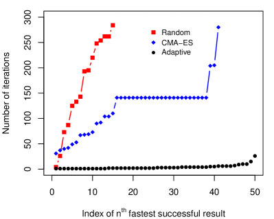
Figure 2. Relative performance of falsification algorithms with AFC27 powertrain requirement: fewer iterations and more successful results are better.

4.4. Discussion

For AT1, aLVTS quickly finds the falsifying input signal, as the required throttle of $100$ and brake of $0$ are contained in level 0 and are very likely to be tried early on. In contrast, even though this is a problem that is well-suited to hill-climbing, CMA-ES has some overhead to sample its initial population, as clearly visible in fig. 3(a).

While CMA-ES deals very well with AT2 for $i=3$, it struggles to find falsifying inputs for $i=4$ (cf. figs. 3(b) and 3(c)). We attribute this to the fact that reaching gear 4 by chance occurs rarely in the exploration of CMA-ES when the robustness score is uninformative. aLVTS not only explores the spatial dimensions, but takes opportunistic jumps to later time points, which increases the probability of discovering a trace (prefix) where the gear is reached.

A priori, one would expect CMA-ES to perform well with AT3 and AT4, exploiting its continuous optimization to fine tune inputs between conflicting requirements. E.g., AT3 requires that $v$ is both above $50$ and below $60$; AT4 requires that $v$ is high while maintaining low $\omega$, which is proportional to $v$. One would similarly expect the limited discrete choices made by aLVTS to hinder its ability to find falsifying inputs. Despite these expectations, our results demonstrate that in most situations aLVTS converges to a falsifying input more consistently and with fewer iterations than CMA-ES. We speculate that this is because CMA-ES is too slow to reach the “sweet spots” in the input space, where its optimization is efficient.

For AT3, there are a few instances where where aLVTS does not quickly find a good prefix towards the corridor $v\in[50,60]$ at time 10 (the rightmost points in fig. 3(d)), which can be explained by the probabilistic nature of the search.

Regarding two instances of AT4 in figs. 3(e) and 3(f), , the graph for aLVTS is generally smoother and shallower, whereas CMA-ES shows consistent performance for only some of the trials but takes significantly more time on the worst 10 trials. We remark that the two parameter settings seem to pose opposite difficulty for the two algorithms, as CMA-ES is significantly quicker for two thirds of the trials for the second instance. It is unclear what causes this variation in performance of CMA-ES.

The plateaux apparent in some of the results using CMA-ES are difficult to explain, but suggest some kind of procedural logic or counter to decide termination. In contrast, the curves for random sampling and aLVTS are relatively smooth, reflecting their purely probabilistic natures.

5. Related Work

The idea to find falsifying inputs using robustness as an optimization function for global optimization originates from (Fainekos and Pappas, 2009) and has since been extended to the parameter synthesis problem (e.g., (Jin et al., 2015)). Two mature implementations in MATLAB are S-Taliro (Annpureddy et al., 2011) and Breach (Donzé, 2010), which have come to define the benchmark in this field. We describe their optimization algorithms below. Approaches to make the robustness semantics more informative are (Eddeland et al., 2017; Akazaki and Hasuo, 2015). These use integrals instead of min/max in the semantics of temporal operators.

Underminer (Balkan et al., 2017) is a recent falsification tool that learns the (non-) convergence of a system to direct falsification and parameter mining. It supports STL formulas, SVMs, neural nets, and Lyapunov-like functions as classifiers. Other global approaches include (Adimoolam et al., 2017), which partitions the input space into sub-regions from which falsification trials are run selectively. This method uses coverage metrics to balance exploration and exploitation. Comprehensive surveys of simulation based methods for the analysis of hybrid systems are given in (Kapinski et al., 2016; Bartocci et al., 2018).

Users of S-Taliro and Breach can select from a range of optimization algorithms (Uniform Random, Nelder-Mead, Simulated Annealing, Cross-Entropy, CMA-ES). These cover a variety of trade-offs between exploration of the search space and exploitation of known good intermediate results. As such, their performance varies with the structure of the problem at hand.

In general, global optimization needs to find a solution in an unstructured combinatorial search space, where the different parameters are assumed, a priori, to be independent. Good combinations of parameter choices have to be discovered first, before the optimization can work effectively (cf. AT2 and AT3). This incurs an exponential cost of exhausting the different combinations, which is mitigated in different ways by the various algorithms. Nelder-Mead is seeded by a constant number of samples and tries to obtain better points in the search space by making linear combinations of the previous ones, according to a fixed scheme. The price paid is not just lack of exploration, but also the danger of selecting mid points between good and bad values in some dimensions, as a consequence of the weighted average of linear combinations. To this end, Cross-Entropy methods and CMA-ES discover relations between parameters and exploit these by decorrelating the choices across independent dimensions (i.e., not trying all possible combinations), as explained nicely in the context of falsification in (Sankaranarayanan and Fainekos, 2012). Simulated Annealing, on the other hand, relies on fairly unguided random exploration, and thus requires many iterations to converge, which can be prohibitively expensive for complex models.

In comparison, our approach explicitly takes into account the temporal structure of the falsification problem. The exponential search space is pruned by focusing on the early part of the input signal, by investigating a small number of coarse choices first, and by ignoring those prefixes which are unpromising according to the robustness heuristic. As demonstrated by our experiments, the strength of optimization algorithms to discover precise solutions in the continuous input space does not seem efficient when the mass of falsifying traces is large and exploration is the key factor.

The characteristic of our approach to explore the search space incrementally is shared with rapidly-exploring random trees (RRTs). The so-called star discrepancy metric guides the search towards unexplored regions and a local planner extends the tree at an existing node with a trajectory segment that closely reaches the target point. RRTs have been used successfully in robotics (LaValle and Kuffner Jr, 2001) and also in falsification (Dreossi et al., 2015). On the other hand, the characteristic of taking opportunistic coarse jumps in time is reminiscent of stochastic local search (Deshmukhand et al., [n. d.]) and multiple-shooting (Zutshi et al., 2014).

Monte Carlo tree search (MCTS) has been applied to a model of aircraft collisions in (Lee et al., 2015); and in a falsification context more recently (Zhang et al., 2018b) to guide global optimization, building on the previous idea of time-staging (Zhang et al., 2018a). That work noted the strong similarities between falsification using MCTS and statistical model checking (SMC) using importance splitting (Jegourel et al., 2013). The robustness semantics of STL, used in (Zhang et al., 2018a; Zhang et al., 2018b) and the present approach to guide exploration, can be seen as a “heuristic score function” (Jegourel et al., 2014) in the context of importance splitting. All these approaches construct trees from traces that share common prefixes deemed good according to some heuristic. The principal difference is that importance splitting aims to construct a diverse set of randomly-generated traces that all satisfy a property (equivalently, falsify a negated property), while falsification seeks a single falsifying input. The current work can be distinguished from standard MCTS and reinforcement learning (Sutton and Barto, 2018) for similar reasons. These techniques tend to seek optimal policies that make good decisions in all situations, unnecessarily covering the entire search space.

6. Conclusion

We have presented a probabilistic algorithm that finds inputs to a hybrid system that falsify a given temporal logic requirement. On standard benchmarks our algorithm significantly and consistently outperforms existing methods. While the falsification problem is inherently hard (no theoretically best solution can exist), we believe that we have found an approach that gives good results in practice, with probabilistic certainty. We believe the reason it works well stems from a property shared by many falsification problems, namely, that there tends to be a significant mass of falsifying inputs. By design it scales with the difficulty of the problem, finding trivial solutions (extreme inputs) immediately and has a small constant overhead for “almost easy” problems. This pays off, in particular, for system models that are expensive to simulate, such as the powertrain benchmark. The approach admits incremental computation of simulations and can easily be parallelized.

As future work, we wish to extend the method with some form of optimization, e.g., by interpolation of previously seen traces, reminiscent of the linear combinations computed by Nelder-Mead. We expect that this would help to “fine-tune” results with small positive robustness into full solutions, mitigating the limitation inherent in the discretization of the input space. Likewise, extrapolation of results could be used to propagate the robustness from one level to the next, reducing the need to look at different branches with similar inputs. Finally, we plan to apply the approach to more benchmarks, specifically those that combine discrete and continuous input domains.

Figure 3. Performance comparison for the automatic transmission benchmark

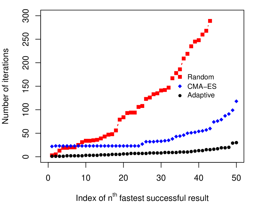
(a) Performance plot for AT1

(b) Performance plot for AT2 $(i=3)$

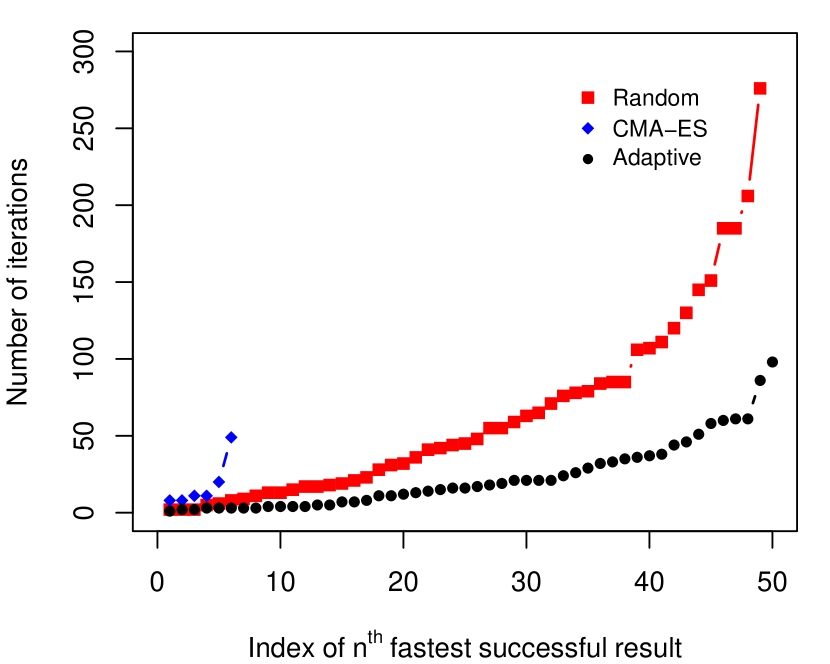
(c) Performance plot for AT2 $(i=4)$

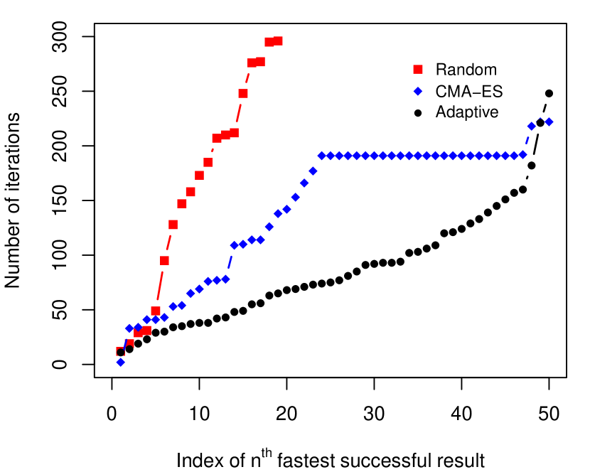
(d) Performance plot for AT3

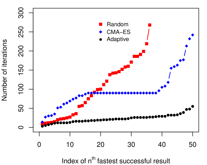
(e) Performance plot for AT4 $(\overline{v}=80,\underline{\omega}=4500)$

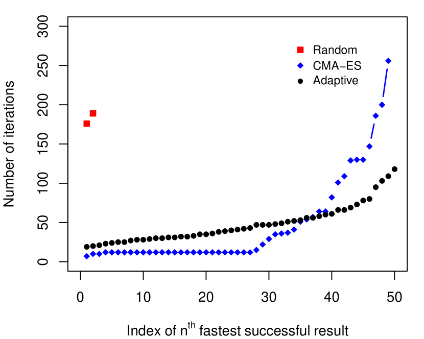
(f) Performance plot for AT4 $(\overline{v}=50,\underline{\omega}=2700)$

- (1)
- Adimoolam et al. (2017) Arvind Adimoolam, Thao Dang, Alexandre Donzé, James Kapinski, and Xiaoqing Jin. 2017. Classification and Coverage-Based Falsification for Embedded Control Systems. In Computer Aided Verification, Rupak Majumdar and Viktor Kunčak (Eds.). Springer, Cham, 483–503.
- Akazaki (2016) Takumi Akazaki. 2016. Falsification of Conditional Safety Properties for Cyber-Physical Systems with Gaussian Process Regression. In Runtime Verification (RV), Yliès Falcone and César Sánchez (Eds.). LNCS, Vol. 10012. Springer, 439–446.
- Akazaki and Hasuo (2015) Takumi Akazaki and Ichiro Hasuo. 2015. Time robustness in MTL and expressivity in hybrid system falsification. In Computer Aided Verification (CAV) (LNCS), Vol. 9207. Springer, 356–374.
- Annpureddy et al. (2011) Yashwanth Annpureddy, Che Liu, Georgios Fainekos, and Sriram Sankaranarayanan. 2011. S-TaLiRo: A Tool for Temporal Logic Falsification for Hybrid Systems. In Tools and Algorithms for the Construction and Analysis of Systems (TACAS) (LNCS), Parosh Aziz Abdulla and K. Rustan M. Leino (Eds.). Springer, 254–257.
- Balkan et al. (2017) Ayca Balkan, Paulo Tabuada, Jyotirmoy V. Deshmukh, Xiaoqing Jin, and James Kapinski. 2017. Underminer: A Framework for Automatically Identifying Nonconverging Behaviors in Black-Box System Models. ACM Trans. Embed. Comput. Syst. 17, 1, Article 20 (2017), 28 pages.
- Barrett et al. (2017) Clark Barrett, Pascal Fontaine, and Cesare Tinelli. 2017. The SMT-LIB Standard: Version 2.6. Technical Report. Department of Computer Science, The University of Iowa. Available at www.SMT-LIB.org.
- Bartocci et al. (2018) Ezio Bartocci, Jyotirmoy Deshmukh, Alexandre Donzé, Georgios Fainekos, Oded Maler, Dejan Ničković, and Sriram Sankaranarayanan. 2018. Specification-based monitoring of cyber-physical systems: a survey on theory, tools and applications. In Lectures on Runtime Verification. Springer, 135–175.
- Deshmukhand et al. ([n. d.]) Jyotirmoy Deshmukhand, Xiaoqing Jin, James Kapinski, and Oded Maler. [n. d.]. Stochastic Local Search for Falsification of Hybrid Systems. Automated Technology for Verification and Analysis (ATVA) 9364 ([n. d.]), 500–517.
- Dokhanchi et al. (2017) Adel Dokhanchi, Shakiba Yaghoubi, Bardh Hoxha, and Georgios E. Fainekos. 2017. ARCH-COMP17 Category Report: Preliminary Results on the Falsification Benchmarks. In Applied Verification of Continuous and Hybrid Systems (ARCH) (EPiC Series in Computing), Goran Frehse and Matthias Althoff (Eds.), Vol. 48. EasyChair, 170–174.
- Dokhanchi et al. (2019) Adel Dokhanchi, Shakiba Yaghoubi, Bardh Hoxha, Georgios E. Fainekos, Gidon Ernst, Zhenya Zhang, Paolo Arcaini, Ichiro Hasuo, and Sean Sedwards. 2019. ARCH-COMP18 Category Report: Results on the Falsification Benchmarks. In Applied Verification of Continuous and Hybrid Systems (ARCH) (EPiC Series in Computing), Goran Frehse (Ed.), Vol. 54. EasyChair, 104–109.
- Donzé (2010) Alexandre Donzé. 2010. Breach, A toolbox for verification and parameter synthesis of hybrid systems. In International Conference on Computer Aided Verification (CAV 2010) (LNCS). Springer, 167–170.
- Donzé et al. (2013) Alexandre Donzé, Thomas Ferrère, and Oded Maler. 2013. Efficient Robust Monitoring for STL. In Computer Aided Verification (CAV) (LNCS), Natasha Sharygina and Helmut Veith (Eds.), Vol. 8044. Springer, 264–279.
- Donzé and Maler (2010) Alexandre Donzé and Oded Maler. 2010. Robust Satisfaction of Temporal Logic over Real-Valued Signals. In Formal Modeling and Analysis of Timed Systems (FORMATS 2010) (LNCS), Krishnendu Chatterjee and Thomas A. Henzinger (Eds.). Springer, 92–106.
- Dreossi et al. (2015) Tommaso Dreossi, Thao Dang, Alexandre Donzé, James Kapinski, Xiaoqing Jin, and Jyotirmoy V. Deshmukh. 2015. Efficient Guiding Strategies for Testing of Temporal Properties of Hybrid Systems. In NASA Formal Methods (NFM) (LNCS), Klaus Havelund, Gerard Holzmann, and Rajeev Joshi (Eds.), Vol. 9058. Springer, 127–142.
- Eddeland et al. (2017) Johan Eddeland, Sajed Miremadi, Martin Fabian, and Knut Åkesson. 2017. Objective functions for falsification of signal temporal logic properties in cyber-physical systems. In Conference on Automation Science and Engineering (CASE). IEEE, 1326–1331.
- Fainekos and Pappas (2009) Georgios E. Fainekos and George J. Pappas. 2009. Robustness of temporal logic specifications for continuous-time signals. Theor. Comp. Sci. 410, 42 (2009), 4262–4291.
- Fleming and Wallace (1986) Philip J Fleming and John J Wallace. 1986. How not to lie with statistics: the correct way to summarize benchmark results. Commun. ACM 29, 3 (1986), 218–221.
- Hoxha et al. (2014) Bardh Hoxha, Houssam Abbas, and Georgios E. Fainekos. 2014. Benchmarks for Temporal Logic Requirements for Automotive Systems. In Applied veRification for Continuous and Hybrid Systems (ARCH) (EPiC Series in Computing), Goran Frehse and Matthias Althoff (Eds.), Vol. 34. EasyChair, 25–30.
- Igel et al. (2007) Christian Igel, Nikolaus Hansen, and Stefan Roth. 2007. Covariance matrix adaptation for multi-objective optimization. Evolutionary computation 15, 1 (2007), 1–28.
- Jegourel et al. (2013) Cyrille Jegourel, Axel Legay, and Sean Sedwards. 2013. Importance Splitting for Statistical Model Checking Rare Properties. In Computer Aided Verification (CAV). LNCS, Vol. 8044. Springer, 576–591.
- Jegourel et al. (2014) Cyrille Jegourel, Axel Legay, and Sean Sedwards. 2014. An Effective Heuristic for Adaptive Importance Splitting in Statistical Model Checking. In Leveraging Applications of Formal Methods, Verification and Validation. Specialized Techniques and Applications (ISoLA), Tiziana Margaria and Bernhard Steffen (Eds.). LNCS, Vol. 8803. Springer, 143–159.
- Jin et al. (2014) Xiaoqing Jin, Jyotirmoy V. Deshmukh, James Kapinski, Koichi Ueda, and Kenneth R. Butts. 2014. Powertrain control verification benchmark. In Hybrid Systems: Computation and Control (HSCC), Martin Fränzle and John Lygeros (Eds.). ACM, 253–262.
- Jin et al. (2015) Xiaoqing Jin, Alexandre Donzé, Jyotirmoy V Deshmukh, and Sanjit A Seshia. 2015. Mining requirements from closed-loop control models. IEEE Transactions on Computer-Aided Design of Integrated Circuits and Systems 34, 11 (2015), 1704–1717.
- Kapinski et al. (2016) James Kapinski, Jyotirmoy V. Deshmukh, Xiaoqing Jin, Hisahiro Ito, and Ken Butts. 2016. Simulation-Based Approaches for Verification of Embedded Control Systems: An Overview of Traditional and Advanced Modeling, Testing, and Verification Techniques. IEEE Control Systems Magazine 36, 6 (Dec 2016), 45–64.
- Kocsis and Szepesvári (2006) Levente Kocsis and Csaba Szepesvári. 2006. Bandit Based Monte-Carlo Planning. In Machine Learning (ECML 2006) (LNCS), Johannes Fürnkranz, Tobias Scheffer, and Myra Spiliopoulou (Eds.), Vol. 4212. Springer, 282–293.
- LaValle and Kuffner Jr (2001) Steven M LaValle and James J Kuffner Jr. 2001. Randomized kinodynamic planning. The International Journal of Robotics Research (IJRR) 20, 5 (2001), 378–400.
- Lee et al. (2015) Ritchie Lee, Mykel J. Kochenderfer, Ole J. Mengshoel, Guillaume P. Brat, and Michael P. Owen. 2015. Adaptive stress testing of airborne collision avoidance systems. In IEEE/AIAA 34th Digital Avionics Systems Conference (DASC 2015). 6C2:1–6C2:13.
- Sankaranarayanan and Fainekos (2012) Sriram Sankaranarayanan and Georgios Fainekos. 2012. Falsification of temporal properties of hybrid systems using the cross-entropy method. In Hybrid Systems: Computation and Control (HSCC). ACM, 125–134.
- Sutton and Barto (2018) Richard S. Sutton and Andrew G. Barto. 2018. Reinforcement Learning: An Introduction (second ed.). MIT press.
- Wolpert and Macready (1997) David Wolpert and William G. Macready. 1997. No free lunch theorems for optimization. IEEE Trans. Evolutionary Computation 1, 1 (1997), 67–82.
- Zhang et al. (2018a) Zhenya Zhang, Gidon Ernst, Ichiro Hasuo, and Sean Sedwards. 2018a. Time-Staging Enhancement of Hybrid System Falsification. In 2018 IEEE Workshop on Monitoring and Testing of Cyber-Physical Systems (MT-CPS 2018). IEEE, 3–4.
- Zhang et al. (2018b) Zhenya Zhang, Gidon Ernst, Sean Sedwards, Paolo Arcaini, and Ichiro Hasuo. 2018b. Two-Layered Falsification of Hybrid Systems Guided by Monte Carlo Tree Search. IEEE Transactions on Computer-Aided Design of Integrated Circuits and Systems (TCAD 2018) (2018).
- Zutshi et al. (2014) Aditya Zutshi, Jyotirmoy V. Deshmukh, Sriram Sankaranarayanan, and James Kapinski. 2014. Multiple shooting, CEGAR-based falsification for hybrid systems. In Embedded Software (EMSOFT). 5:1–5:10.