University of Copenhagen

Master’s Thesis

  Duelling Bandits with Weak Regret in Adversarial Environments  
             Author:              Supervisor:              Lennard Hilgendorf              Yevgeny Seldin              fwc817@alumni.ku.dk              seldin@di.ku.dk
August 6, 2018

Abstract

Research on the multi-armed bandit problem has studied the trade-off of exploration and exploitation in depth. However, there are numerous applications where the cardinal absolute-valued feedback model (e.g. ratings from one to five) is not suitable. This has motivated the formulation of the duelling bandits problem, where the learner picks a pair of actions and observes a noisy binary feedback, indicating a relative preference between the two. There exist a multitude of different settings and interpretations of the problem for two reasons. First, due to the absence of a total order of actions, there is no natural definition of the best action. Existing work either explicitly assumes the existence of a linear order, or uses a custom definition for the winner. Second, there are multiple reasonable notions of regret to measure the learner’s performance. Most prior work has been focussing on the strong regret, which averages the quality of the two actions picked. This work focusses on the weak regret, which is based on the quality of the better of the two actions selected. Weak regret is the more appropriate performance measure when the pair’s inferior action has no significant detrimental effect on the pair’s quality.

We study the duelling bandits problem in the adversarial setting. We provide an algorithm which has theoretical guarantees in both the utility-based setting, which implies a total order, and the unrestricted setting. For the latter, we work with the Borda winner, finding the action maximising the probability of winning against an action sampled uniformly at random. The thesis concludes with experimental results based on both real-world data and synthetic data, showing the algorithm’s performance and limitations.

Notation

Symbol	Definition
$\mathbb{E}\left[\cdot\right]$	Expectation of random variable
$\mathbbm{1}\left(\cdot\right)$	Indicator function
$\Delta^{K}$	$K$-simplex
$[K]$	Set $\left\{1,\ldots,K\right\}$
$K$	Number of arms
$T$	Time horizon
$\mathbf{M}^{t}$	Outcome matrix in round $t$
$\mathcal{M}$	Sequence of outcome matrices
$\bm{\ell}_{t}$	Loss vector in round $t$
$\mathcal{L}$	Sequence of loss vectors
$A_{t},B_{t}$	Pair of actions played in round $t$
$Y_{t}$	Outcome observed in round $t$
$\psi(\cdot,\cdot)$	Loss-combining function
$R(T)$	Cumulative regret until round $T$
$\phi(\cdot,\cdot)$	Link function
$\mathbf{x}$	Reward / utility vector
$a_{U}^{*}$	Utility-based winner
$a_{B}^{*}$	Borda winner
$a_{C}^{*}$	Copeland winner
$\mathbf{u}$	Von-Neumann winner
$R_{S}(T)$	Cumulative strong regret
$R_{W}(T)$	Cumulative weak regret
$R_{W}^{U}(T)$	Utility-based cumulative weak regret
$R_{W}^{N}(T)$	Non-utility-based cumulative weak regret
$\eta$	Learning rate
$\widetilde{\ell}^{a}$	Loss estimator
$\widetilde{L}_{t}(a)$	Cumulative loss estimator
$\mathcal{H}_{t}$	Set $(A_{1},B_{1},Y_{1}),\ldots,(A_{t},B_{t},Y_{t})$
$\bar{\bm{\ell}}_{t}$	Utility-based loss vector in round $t$

Chapter 1 Introduction

The trade-off between exploration and exploitation, which arises in various sequential decision problems and online learning problems such as reinforcement learning, has been studied in-depth by research on the multi-armed bandit problem. Given a set of actions, which are also termed arms, the environment assigns a bounded real-valued utility to each of them. Following a sequential game protocol, the learner picks an arm and observes its noisy real-valued feedback, which is based on the arm’s utility. The learner’s goal is to maximise the cumulative reward. This theoretical framework can be applied to various practical settings where cardinal feedback is readily available.

However, often other feedback models are required. In the context of online ranker evaluation, Radlinski et al. (2008) examined the relation between various absolute usage metrics and the quality of retrieval functions. They concluded that none of the measures covered were a reliable predictor for the retrieval quality. Instead, their results suggested that relative feedback obtained through pairwise comparisons, such as “option A is preferred over option B”, can be used for consistent and more accurate estimates. Often this form of feedback is easier to obtain, making it desirable to have algorithms which are capable of handling this learning task.

Research addressing the duelling bandits problem deals with formalisation of online learning problems involving pairwise comparisons and studies algorithms selecting a sequence of pairs of actions, assuming a binary feedback mechanism. The term has been coined by Yue and Joachims (2009), who were motivated by the results of the experimental studies by Radlinski et al. (2008).

Unlike the classical multi-armed bandit problem, the existence of a linear order is not guaranteed, as violations of transitivity ($A\succ B\succ C\succ A$) cannot be ruled out. This makes the definition of a winner ambiguous. The first papers either explicitly assumed a linear order, or used a convex utility-function, which in turn induces a total order. Yue and Joachims (2009) modelled the space of actions $\mathcal{W}$ as a convex subset of the $d$-dimensional Euclidean space, allowing the embedding of the parameterisation of complex retrieval functions. Assuming a convex function mapping actions to real-valued utilities, outcomes of comparisons between two actions are modelled as independent Bernoulli random variables with bias given by an odd link function mapping the signed difference of two utilities to the zero-one interval. In order to measure the performance of an algorithm, they introduced a notion of regret, which corresponds to what subsequent literature terms as strong regret (Yue et al., 2012). Given a finite time horizon $T$, strong regret relates to the cumulative difference between the average quality of the pair of actions chosen at time $t$ and the quality of the best action in hindsight $a^{*}$, which has maximum utility. This measure reflects the relative number of users who would have chosen the best action over an action picked uniformly at random from the pair of actions (Yue et al., 2012), and is zero in this setting if and only if both actions selected are the best action.

Instead of considering an infinite space of parameterisations, it is often more sensible to consider a more limited set of actions. Presuming that this set of actions is finite, i.e. $\left\lvert\mathcal{W}\right\rvert=K$, Yue et al. (2012) examine the $K$-armed duelling bandits problem. Instead of relying on a utility function, they assumed the existence of a total order of the set of actions. Complementing the previously defined strong regret, they introduced the notion of weak regret, which reflects the relative number of users preferring the overall best arm over the better action of the pair of actions presented. To be zero, it suffices that the better action is identical to the best action.

In practice, the assumption of a total order is often violated, limiting the works’ applicability (Dudík et al., 2015). Some works assume the existence of a Condorcet winner, which is an action winning against all other actions with probability $>\frac{1}{2}$. Urvoy et al. (2013) dropped the assumption of utilities and linear orders altogether, giving rise to the stochastic non-utility-based duelling bandits problem. Recognising that this relaxation might impede the existence of a Condorcet winner, they resort to the corpus of social choice theory and voting theory, basing the definition of the winner and the mechanism inducing regret on the Borda score, which relates to the probability of a particular action winning against an action sampled uniformly at random, as well as on the Copeland score, which takes into account the number of other actions an action is preferred to. The latter has been covered in greater extent by Zoghi et al. (2015) as a natural generalisation of the Condorcet winner. A game-theoretic interpretation of the duelling bandits problem was initially suggested by Dudík et al. (2015). In an attempt to address certain shortcomings of the Borda winner and the Copeland winner, they introduced the notion of the von-Neumann winner, which is a distribution over actions which beats every other policy with probability $\geq\frac{1}{2}$. In addition, they discussed the case where outcomes are no longer sampled from a stationary distribution, but instead are generated from a distribution which is selected by an adversary in an arbitrary way on a per-round basis.

The adversarial duelling bandits problem was further studied by Gajane et al. (2015), who assumed a binary utility vector, effectively splitting the set of actions into a set of “good” actions and a set of “bad” actions, the former winning all duels against the latter with probability one.

Finally, Chen and Frazier (2017) revisited the notion of weak regret by Yue et al. (2012), proving bounds on the expected regret constant in $T$, assuming a Condorcet winner.

	Stochastic Setting	Adversarial Setting
Utility-based setting	Yue and Joachims (2009) Yue et al. (2012) Ailon et al. (2014) Chen and Frazier (2016) Chen and Frazier (2017)	Gajane et al. (2015) This work
Condorcet winner	Yue and Joachims (2011) Urvoy et al. (2013) Zoghi et al. (2014) Komiyama et al. (2015) Chen and Frazier (2017)
Borda winner	Urvoy et al. (2013) Jamieson et al. (2015)	This work
Copeland winner	Urvoy et al. (2013) Zoghi et al. (2015) Wu and Liu (2016)
Von-Neumann winner	Balsubramani et al. (2016)	Dudík et al. (2015)

Table 1.1: Overview of existing work

As shown in the summary in Table 1.1, most prior work has been focussing on the strong regret to evaluate the quality of pairs of actions. The suitability of the strong regret depends on the application and assumption made: if the presence of undesired actions has a negative impact on the perceived quality or if the user’s experience can be enhanced by showing two good options, e.g. when considering search results (Chen and Frazier, 2017), strong regret is a reasonable modelling assumption. However, if the quality of pairs consisting of a good and a bad action is dominated by the quality of the former, it might be more appropriate to consider the weak regret. At the same time, the requirement that outcomes are sampled from a stationary distribution might not always be adequate in practice. To our knowledge, algorithms for weak regret have only been devised in the stochastic setting requiring a Condorcet winner. So far studies of the adversarial duelling bandits problem have been limited to the von-Neumann setting and, with with some limitations, the utility-based setting, limiting its practical applicability.

This work provides a framework consolidating the different problem formulations, facilitating discussion of results by relating the utility-based setting to the non-utility-based setting. Subsequently, we discuss the suitability of a range of algorithms assuming different winner models and support our claims experimentally. Finally, we propose an algorithm covering both the utility-based setting and the non-utility-based setting of the adversarial duelling bandits problem, the latter using the Borda winner to define the winner and quality of individual actions. We restrict ourselves to weak regret, proving an upper bound on the expected regret of $O\left(\sqrt{KT\log K}\right)$, extending the work on adversarial duelling bandits by Dudík et al. (2015) and Gajane et al. (2015), covering a different winner setting and regret measure. Our contribution advances the applicability of duelling bandits algorithms by providing a robust algorithm with explicit regret guarantees in adversarial settings.

The remainder of this thesis is structured as follows: Chapter 2 covers related literature in greater detail than the summary above. Chapter 3 formalises the problem setting and introduces the notation used in subsequent chapters. Chapter 4 presents existing algorithms referenced in later chapters as well as our algorithmic contribution, whose theoretical analysis is presented in Chapter 5. Our experimental evaluation of the algorithms under different performance measures is included in Chapter 6. Chapter 7 concludes this thesis with a discussion of our work.

Chapter 2 Prior Work

This chapter covers the most relevant algorithms for the classical multi-armed bandit problem, as well as the prior research on the duelling bandits problem.

2.1 Multi-Armed Bandit (MAB) Problem

This section summaries algorithms relevant for the remainder of this thesis which address the finite multi-armed bandit problem.

2.1.1 Exponential-weight Algorithm for Exploration and Exploitation (Exp3)

There are scenarios where the assumption of a stationary distribution is not viable. Proposed by Auer et al. (2003), the adversarial or non-stationary bandit problem makes no assumption about the process generating the sequence of rewards. Their simplest algorithm Exp3 is an exponential-weights algorithm. It maintains a vector of weights, which are mapped to a probability distribution $p_{t}$ using the softmax function. Every round an action is sampled from this distribution, its associated reward is observed, and the weight vector is updated. The original algorithm is controlled through a parameter $\gamma\in(0,1]$, which controls the weight of a uniform exploration component. Other variants (Bubeck and Cesa-Bianchi, 2012) use a learning rate $\eta$ instead, which allows for a more elegant analysis. This work adopts the latter approach, as seen in Algorithm 1 and Algorithm 2. Both $\gamma$ and $\eta$ depend on the time horizon $T$. To make Exp3 suitable for the anytime setting, a variable learning rate $\eta_{t}$ can be used. Assuming that the time horizon $T$ is known and that the rewards are bounded by the zero-one interval, the expected regret of Exp3 using $\eta=\sqrt{\frac{2\log K}{TK}}$ is bounded by $O(\sqrt{2KT\log K})$ (Bubeck and Cesa-Bianchi, 2012).

2.1.2 Exp3.P

Exp3 multiplies the outcome observed after playing action $i$ with $\frac{1}{p_{t}^{i}}$, compensating for the sampling process to obtain an unbiased estimate. The lack of a lower bound of $p_{t}^{i}$ introduces a potentially large variance to the estimates, rendering it impossible to derive any interesting high-probability bounds on the algorithm’s regret. Exp3.P (Auer et al., 2003) resolves this issue by effectively adding a bias term to the aforementioned estimates. The variation presented by Bubeck and Cesa-Bianchi (2012) comes along with different high-probability bounds, depending on the parameterisation used. The simplest bound guarantees that with probability greater than $1-\delta$, the algorithm’s regret is bounded by $5.15\sqrt{KT\log{\frac{K}{\delta}}}$ when using the parameters required by (Bubeck and Cesa-Bianchi, 2012, Theorem 3.2). This variant of Exp3.P was used in Algorithm 3.

2.2 Duelling Bandits Problem

As discussed in Chapter 1 and summarised in Table 1.1, the duelling bandits problem has been analysed in various settings under different assumptions. As these have a substantial impact on the nature of the problem, we structure this chapter accordingly.

2.2.1 Utility-based Setting

In the utility-based setting, every action is assigned a real-valued utility. Outcomes of duels are modelled as Bernoulli random variables, whose bias is determined by a known link function, which maps pairs of utilities to the zero-one interval. This link function is assumed to induce a total order.

Dueling Bandit Gradient Descent (DBGD)

The first formalisation of the duelling bandits problem was proposed by Yue and Joachims (2009), who modelled the space of actions $\mathcal{W}$ as a convex, bounded, and closed space contained in a ball with finite radius $R$ in $d$-dimensional Euclidean space. The outcome of any pairwise comparison between two actions $w_{1},w_{2}\in\mathcal{W}$ is modelled as an independent Bernoulli random variable with bias $\sigma(v(w_{1})-v(w_{2}))$, assuming a strictly concave utility function $v\colon\mathcal{W}\to\mathbb{R}$ and a rotation-symmetric, monotonic increasing link function $\sigma\colon\mathbb{R}\to[0,1]$ with $\sigma(-\infty)=0$, $\sigma(0)=\frac{1}{2}$, and $\sigma(\infty)=1$, both functions satisfying some mild smoothness assumptions. These assumptions give rise to a unique best action $w^{*}$, which is preferred to every other action with probability $>\frac{1}{2}$. This property makes $w^{*}$ a Condorcet winner. The bias of the Bernoulli random variables induces a gap function $\epsilon\colon\mathcal{W}\times\mathcal{W}\to[-\frac{1}{2},\frac{1}{2}]$:

$$\forall w_{i},w_{j}\in\mathcal{W}:\epsilon(w_{i},w_{j})=\sigma(v(w_{i})-v(w_{j}))-\frac{i}{j}=\Pr\left[w_{i}\succ w_{j}\right]-\frac{i}{j},$$

which they use to define the performance measure of an algorithm selecting pairs for comparison. The event $w_{i}\succ w_{j}$ is equivalent to “action $w_{i}$ beats action $w_{j}$ in a specific duel”. They use the notation of regret as performance measure of an algorithm, which accumulates the gaps between the best action in hindsight $w^{*}$ and the two actions picked. Given a finite time horizon $T$, they define the regret after $T$ rounds

$$R(T)=\sum_{t=1}^{T}\left[\epsilon(w^{*},A_{t})+\epsilon(w^{*},B_{t})\right],$$ (2.1)

where $A_{t},B_{t}\in\mathcal{W}$ denote the pair of actions picked in round $t$.

They propose the algorithm DBGD and prove an upper bound on the expected regret sublinear in $T$ with $O(T^{3/4}\sqrt{Rd})$. In the information retrieval setting, DBGD allows complex parameterised retrieval functions to be embedded in $\mathcal{W}$, with the algorithm exploring different parameterisations.

Interleaved Filter (IF)

Instead of considering a continuous space of actions, Yue et al. (2012) proposed the $K$-armed duelling bandits problem, a variant considering a finite space of $K$ actions. They coined the terms strong regret and weak regret. The former corresponds to the definition presented in (2.1), while they defined weak regret as

$$\widetilde{R}(T)=\sum_{t=1}^{T}\min\left\{\epsilon(w^{*},A_{t}),\epsilon(w^{*},B_{t})\right\}.$$

Adapting an explore-then-exploit approach, they proposed two tournament elimination-based algorithms named IF1 and IF2. Both algorithms start out with a random candidate action $\hat{b}$ and a pool of remaining actions $W=\mathcal{W}\setminus\{\hat{b}\}$. They maintain an estimate $\hat{P}_{\hat{b},b}$ of the candidate action’s superiority to every action $b\in W$, as well as a confidence interval $\hat{C}_{\hat{b},b}$, which encompasses the true value $\Pr[\hat{b}>b]$ with probability greater than $1-\delta$, using $\delta=\frac{1}{TK^{2}}$. Every round, the algorithms select an action $b$ from the pool of remaining actions in a round-robin manner, observe the outcome of the duel between $\hat{b}$ and $b$, and update the relevant estimate and confidence interval. Actions are removed from $W$ if their point estimate of inferiority becomes greater than $\frac{1}{2}$ and $\frac{1}{2}\notin\hat{C}_{\hat{b},b}$. On the other hand, if an action $b$’s estimate of inferiority falls below $\frac{1}{2}$ and $\frac{1}{2}\notin\hat{C}_{\hat{b},b}$, then $b$ is removed from $W$ and replaces the candidate action. All estimates and confidence intervals are reset, and the algorithms repeat until the pool $W$ is empty, transitioning to the exploitation phase by playing the pair $(\hat{b},\hat{b})$. IF2 adds a pruning step, which eliminates all actions $b$ with $\hat{P}_{\hat{b},b}\succ\frac{1}{2}$ just before updating the candidate action $\hat{b}$.

They proved that both the strong regret and the weak regret of IF1 and IF2 are bounded by $O\left(\frac{K\log K}{\epsilon_{1,2}}\log T\right)$ and $O\left(\frac{K}{\epsilon_{1,2}}\log T\right)$, respectively, $\epsilon_{1,2}=\Pr\left[w_{1}>w_{2}\right]-\frac{1}{2}$ denoting the distinguishability between the two best actions $w_{1}$ and $w_{2}$.

Doubler, MultiSBM, Sparring

Ailon et al. (2014) introduced the notion of the utility-based duelling bandit problem, assuming that every action induces a stationary distribution with support in $[0,1]$. A duel between two actions $A_{t},B_{t}$ leads to the unobserved reward $\frac{1}{2}\left(u_{t}+v_{t}\right)$, where $u_{t}$ and $v_{t}$ are sampled from the distributions induced by the respective actions. The observable outcome is modelled as Bernoulli random variable with bias by a linear link function

$$\phi_{\mathrm{lin}}(u_{t},v_{t})=\frac{1+v_{t}-u_{t}}{2}.$$ (2.2)

They employed a utility-based definition of regret, which is related to the strong regret (2.1). This assumption allowed the authors to provide different reductions to the classic MAB problem.

Their first algorithm, Doubler, is suitable for both finite sets of $K$ arms and infinite sets, assuming a convex utility function similarly to Yue and Joachims (2009) and a specific link function. We will focus only on the finite case here, as this thesis does not cover the infinite case. Doubler is based on exponentially growing epochs, obsoleting the need to know a time horizon $T$, making it parameter-less. At its core, it uses an instance of an algorithm $S$, which solves a classical MAB problem. The set of actions of $S$ is identical to the duelling bandits problem’s actions. Every round, $S$ is queried, yielding the first item of the pair of actions to be played. For each epoch, Doubler maintains a multi-set of actions selected by $S$. The second action is sampled uniformly at random from the multi-set from the previous epoch, effectively fixing the strategy $S$ plays against for every epoch. The outcome of the duel between the ordered pair is observed and fed back to $S$ as cardinal $\left\{0,1\right\}$ feedback, rewarding picks when they win the duel. Assuming that the MAB algorithm employed is UCB1, they showed that Doubler suffers at most $O\left(\sum_{i=2}^{K}\Delta_{i}^{-1}\log^{2}T\right)$ regret in expectation, where $\Delta_{i}$ denotes the positive difference between the $i$-th best action’s utility and the best action’s utility.

Their second contribution, MultiSBM (Multi Singleton Bandit Machine), improves this result by a logarithmic factor, sacrificing the ability to handle infinite sets of actions. Instead of using a single instance of an MAB algorithm, this approach uses $K$ independent instances $S_{1},\dots,S_{K}$, each featuring $K$ arms. $A_{0}\in\left\{1,\dots,K\right\}$ being in arbitrary action. MultiSBM chooses $A_{t}=B_{t-1}$, basing the first action on the second action played in the previous round. Simultaneously, it queries $S_{A_{t}}$, yielding $B_{t}$. Similar to Doubler, the outcome of the duel is fed back to $S_{A_{t}}$. Using a variant of UCB1, they provided an upper bound of $O(K\log T)$ on the expected strong regret for sufficiently large time horizons.

Lastly, the authors presented an approach using only two instances of MAB algorithms $S_{L}$ and $S_{R}$, which they named Sparring. Every round $t$, $S_{L}$ and $S_{R}$ are queried, yielding the actions $A_{t}$ and $B_{t}$, respectively. The resulting outcome is fed back to both MAB algorithms, inverted accordingly for one of the algorithms. While they did not provide any theoretical regret guarantees, they included it in their experiments and claimed that it outperformed both Doubler and MultiSBM. Due to its potential suitability for the adversarial setting, we have included it in our empirical evaluation.

Relative Exp3 (REX3)

The idea of using two instances of an MAB algorithm was revisited by Gajane et al. (2015), who exmained an adversarial instance of the utility-based duelling bandits problem with $K$ arms. Every round, an adversary fixes a binary utility vector $\mathbf{x}(t)\in\left\{0,1\right\}^{K}$, which, in combination with a link function $\phi(x_{i},x_{j})=x_{i}-x_{j}\in\left\{-1,0,1\right\}$, deterministically determines the outcome of the duel between actions $i$ and $j$. This ternary domain allows the occurrence of draws. Moreover, these are guaranteed to occur if $K>2$, as the assumption of the utilities being binary effectively splits the set of actions into a subset of “good” actions with utility 1, and a subset of “bad” actions with utility 0. Duels between actions from the same subset result in a draw due to the assumption of the link function. The performance measure employed is a utility-based version of strong regret, as used by Ailon et al. (2014).

The algorithm they suggested, REX3, is based on Sparring, using Exp3 as building block with some modifications. Only a single weight vector is used, meaning that a single instance of Exp3, which is queried twice, plays against itself. In case the outcome is non-zero, the weights associated with the winner action and the loser action are increased and decreased, respectively. If a draw is observed, no update to the weight vector is made. Under these assumptions, they prove an upper bound on the expected strong regret of $2\sqrt{eKT\log K}=O(\sqrt{KT\log K})$.

Winner Stays (WS)

Most recently, Chen and Frazier (2016, 2017) extended the study of the stochastic utility-based duelling bandit problem to the setting of weak regret. Chen and Frazier (2017) proposed two algorithms, Winner Stays with Weak Regret (WS-W) and Winner Stays with Strong Regret (WS-S). WS-W maintains a vector $\mathbf{C}\in\mathbb{Z}^{K}$, whose elements $C_{i}$ are counters which are incremented whenever action $i$ wins a duel, and decremented when $i$ loses a duel. Every round it picks $A_{t}=\arg\max_{i}C_{i}$, breaking ties by preferring $A_{t-1}$ and $B_{t-1}$. In case none of the previous actions played maximise $C_{i}$, $A_{t}$ is sampled uniformly from $\arg\max_{i}C_{i}$. $B_{t}$ is selected in a similar manner, excluding $A_{t}$ from the actions available. Upon observation of the outcome the relevant counters are updated.

WS-S builds on this algorithm and makes it applicable to the strong regret setting. Splitting the time axis in exponentially growing epochs, it uses WS-W for the first part of every epoch. This fraction is controlled by a parameter $\beta$ and depends on the epoch. The second part of the epoch is an exploitation phase, which uses the best action determined by the precedent exploration phase. While they did not reference utilities directly, their theoretical analysis of the expected regret proves tighter bounds when assuming a total order, namely $O(K\log K)$ for weak regret and $O(K\log(KT)$ for strong regret.

Comparing The Best (CTB)

Chen and Frazier (2016) made the assumption that each arm $i$ has an observable $d$-dimensional feature vector $\mathbf{A}_{i}$. Assuming an unknown vector $\bm{\theta}\in\mathbb{R}^{d}$, the known utility function $u(\bm{\theta},\mathbf{A}_{i})=\left<\bm{\theta},\mathbf{A}_{i}\right>$ assigns real-valued utilities to them. An exploitable dependence between the arms as well as a total order is induced by a link function. The authors suggest both the Bradley-Terry model

$$\Pr\left[i\succ j\right]=\frac{\exp(u(\bm{\theta},\mathbf{A}_{i}))}{\exp(u(\bm{\theta},\mathbf{A}_{i})+u(\bm{\theta},\mathbf{A}_{j}))}$$ (2.3)

and the probit model

$$\Pr\left[i\succ j\right]=\Phi(u(\bm{\theta},\mathbf{A}_{i})-u(\bm{\theta},\mathbf{A}_{j})),$$ (2.4)

which uses the cumulative distribution function of the normal distribution.

Their algorithm Comparing The Best assigns a score to all $K!$ possible orders, which relates to the posterior distribution of an order being the relevant order based on all previous observations. Every round CTB picks the respective best action of the two orders with maximal score, observes the outcome of the duel, and updates all scores. The authors provided an upper bound of $O(K^{2})$ on the expected weak regret, ignoring any instance-dependent multiplicative constants. Using synthetic datasets, CTB outperformed WS-W as well as and other algorithms which were not explicitly designed for the weak regret setting.

2.2.2 Condorcet Winner

The Condorcet winner setting only makes the assumption that the best arm wins against all other arms, dropping the requirement of a total order. It is therefore a generalisation of the utility-based setting, increasing the model’s applicability.

Beat-The-Mean (BTM)

Yue and Joachims (2011) were the first to propose and examine this relaxed setting. They invented the algorithm Beat-The-Mean, which does not require any transitivity assumptions. A working set of arms $W$ contains initially all $K$ arms. Over $K-1$ epochs, the action in $W$ which has been involved in the least number of comparisons is picked to be $A_{t}$. $B_{t}$ is sampled uniformly at random from the working set. Keeping track of the fraction of duels won and duels played, the action with the lowest empirical performance is removed from the working set when it is ruled out as the Condorcet winner with sufficient confidence. After adjusting the counters keeping track of the individual arms’ performance, the next epoch begins. In case just a single action is left, BTM transitions to its exploitation phase. Ignoring any instance-dependent multiplicative constants, its strong regret in expectation is bounded by $O(K\log T)$. This hides a multiplicative factor of $\frac{\gamma^{7}}{\epsilon_{*}}$, with $\gamma\geq 1$ increasing when transitivity of the actions’ preferences is violated, and $\epsilon_{*}=\min_{i}\epsilon(w^{*},i)$.

Sensitivity Analysis of VAriables for Generic Exploration (SAVAGE)

Unlike all prior work covered so far in this chapter, Urvoy et al. (2013) examines the stochastic duelling bandits problem in a modified version of the PAC setting. Instead of bounding some notion of regret, they provide bounds on the number of rounds SAVAGE requires to terminate, yielding the $\varepsilon$-correct arm with probability greater than $1-\delta$.

Instead of making any explicit assumptions about the winner, SAVAGE uses a “sensitivity analysis subroutine”, which incorporates the definition of the winner, and is used to gradually reduce the working set until all other actions have been eliminated. In the Condorcet winner setting, the winner is found with probability greater than $1-\delta$ in $O\left(K^{2}\log\left(\frac{KT}{\delta}\right)\right)$ when loosening the bound to adjust for instance-dependent constants.

Relative Upper Confidence Bound (RUCB)

Similarly to UCB (Auer et al., 2002), RUCB uses a time-dependent upper confidence bound on the actions’ performance, yielding regret guarantees which hold for any time $t$. The algorithm maintains a matrix $\mathbf{W}\in\mathbb{Z}_{+}^{K\times K}$, whose elements $W_{ij}$ keep track of the number of rounds action $i$ won against action $j$. Given a fixed input parameter $\alpha>\frac{1}{2}$, it constructs a corresponding upper confidence matrix $\mathbf{U}\in\mathbb{R}_{+}^{K\times K}$ with

$$U_{ij}=\frac{W_{ij}}{W_{ij}+W_{ji}}+\sqrt{\frac{\alpha\log t}{W_{ij}+W_{ji}}}$$ (2.5)

if $i\neq j$ and $U_{ii}=\frac{1}{2}$. The first term of (2.5) rewards well-performing actions, while the second term boosts less-played actions, guaranteeing sufficient exploration. A set $\mathcal{C}=\left\{i\middle|\forall j:U_{ij}\geq\frac{1}{2}\right\}$ is updated every round. If it is empty, $A_{t}$ is picked uniformly at random from the set of actions $\left\{1,\dots,K\right\}$. If it contains just a single element, $A_{t}$ assumes this action. Otherwise it is sampled from $\mathcal{C}$ using a custom distribution. Using $B_{t}=\arg\max_{j}U_{jA_{t}}$, the outcome of the duel between $A_{t}$ and $B_{t}$ is observed and $\mathbf{W}$ is updated.

The authors provided an upper bound on the expected strong regret of $O(K\log t)$, which is consistent with the lower bound of the duelling bandits problem in this setting (Yue et al., 2012).

Relative Minimum Empirical Divergence (RMED)

Komiyama et al. (2015) provided a range of algorithms which explicitly make use of the binary Kullback-Leibler divergence. After an initial exploration of all pairs of actions, RMED proceeds to an exploration / exploitation phase. Due to its complexity, we refer to the original paper at this point. The simplest algorithm, RMED1, comes along with a proof of an upper bound on its expected strong regret of $O(K\log T)$. The more complicated algorithm RMED2FH comes along with a proof sketch, which promises a regret bound matching the lower bound provided in the same paper, improving the previously proved bound by a constant factor.

Winner Stays (WS)

When dropping the assumption of a total order, as described in Subsection 2.2.1, Chen and Frazier (2017) showed that the expected weak regret of WS-W is bounded by $O(K^{2})$, while the expected strong regret of WS-S has an upper bound of $O(K^{2}+K\log T)$.

2.2.3 Borda Winner

Unlike the Copeland winner and the von-Neumann winner, which pose a generalisation of the Condorcet winner, the Borda winner is the action maximising the probability of winning a duel sampled from all $K$ actions uniformly at random. This dependence on all other actions implies that the Borda winner is not guaranteed to be the Condorcet winner when the assumption of a total order is not fulfilled.

Sensitivity Analysis of VAriables for Generic Exploration (SAVAGE)

While the Urvoy et al. (2013) were the first to suggest the Borda winner and pointed out that SAVAGE was directly applicable in this setting, they included the Borda winner only in their experimental section. The authors argued that this setting was less complex than the Copeland setting, and could be readily solved by classical MAB algorithms.

Successive Elimination with Comparison Sparsity (SECS)

Jamieson et al. (2015) used the suggestion by Urvoy et al. (2013) to employ a classical MAB algorithm to solve the Borda duelling bandits problem as a baseline, which they termed Borda reduction. SECS exploits different structural assumptions of the constant preference matrix, allowing the identification of the Borda winner in fewer rounds than the Borda reduction, if fulfilled.

2.2.4 Copeland Winner

Instead of requiring an action winning against all other actions with probability greater than $\frac{1}{2}$, the Copeland winner is any action winning against the greatest number of other actions, not taking into account by how much it outperforms them.

Sensitivity Analysis of VAriables for Generic Exploration (SAVAGE)

When applying SAVAGE under the assumption of the existence of a Copeland winner, Urvoy et al. (2013) bound the number of rounds the algorithm requires to yield the winner with probability greater than $1-\delta$ by $O\left(K^{2}\log\left(\frac{KT}{\delta}\right)\right)$.

Copeland Confidence Bounds (CCB), Scalable Copeland Bandits (SCB)

Zoghi et al. (2015) improved on the result above using CCB, which is inspired by RUCB. In addition to the upper confidence bound matrix $\mathbf{U}$, it introduces a lower confidence bound matrix $\mathbf{L}$ and a counter $L_{C}\in\mathbb{N}$ estimating the number of arms the best arm loses against. Furthermore, it maintains a working set $\mathcal{B}_{1}$ of potential Copeland winners and, for every arm $i$, a set of arms $\mathcal{B}_{1}^{i}$ potentially beating $i$. Every round, CCB chooses $A_{t}$ to be an empirically well-performing arm, with arms in $\mathcal{B}_{1}$ more likely to be selected. $B_{t}$ is chosen from $\mathcal{B}_{1}^{A_{t}}$ with the intention of ultimately removing either $A_{t}$ from $\mathcal{B}_{1}$ (if $A_{t}\in\mathcal{B}_{1}$) or $B_{t}$ from $\mathcal{B}_{1}^{A_{t}}$. The algorithm has a multitude of mechanisms controlling the specific mechanism according to which these actions are sampled, which are out of the scope of this summary.

Assuming that there exists no pair of distinct actions $i,j$ for which $\Pr\left[i\succ j\right]=\frac{1}{2}$, the expected strong regret of CCB is bounded by $O(K^{2}+K\log T)$. To remove the quadratic dependence on $K$, which limits the applicability for problem instances with a large number of arms, SCB divides the time axis into epochs of iterated exponentially length. Every epoch, it launches an exploration phase using a variant of CCB. Upon termination of this subroutine, it proceeds with the exploitation phase for the remainder of the epoch, playing twice the approximated Copeland winner. SCB comes along with a upper bound on the expected strong regret of $O(K\log K\log T)$, suggesting better results for larger values of $K$.

Double Thompson Sampling (DT-S)

Motivated by previous applications of Thompson sampling to the MAB problem (Chapelle and Li, 2011), Wu and Liu (2016) presented DT-S, which uses Thompson sampling to select both actions. They proved an upper bound of $O(K^{2}\log T)$ on the expected strong regret in the Copeland setting.

2.2.5 Von-Neumann Winner

The von-Neumann winner stems from a game-theoretic interpretation of the duelling bandits problem. Instead of maximising a pre-defined quality measure such as the probability of winning against an action sampled uniformly at random or the number of actions an arm wins against with probability $>\frac{1}{2}$, the von-Neumann winner is the distribution over all arms winning against any other policy with probability $>\frac{1}{2}$ (Dudík et al., 2015). This definition has two convenient properties. First, it is compatible to the definition of the Condorcet winner. Secondly, unlike the Borda winner and the Copeland winner, it is not influenced by the existence of clones of actions (Dudík et al., 2015).

Sparring Exp4.P, SparringFPL, ProjectedGD

In addition to examining the duelling bandits problem in a novel winner scenario, Dudík et al. (2015) suggested a variant which incorporates context, similar to the classical MAB with expert advice (Auer et al., 2003). They proposed an algorithm of Sparring with two independent instances of Exp4.P, which is a variant of Exp3.P capable of incorporating context (Bubeck and Cesa-Bianchi, 2012). The authors argued that the strong regret of Sparring Exp4.P is bounded by $O\left(\sqrt{KT\frac{\lvert\Pi\rvert}{\delta}}\right)$ with probability greater than $1-\delta$, where $\lvert\Pi\rvert$ denotes the size of the policy space $\Pi$. This bound is holds also for the adversarial setting.

SparringFPL and ProjectedGD are designed for large policy spaces, offering better time and space requirements. We omit them for this summary as this work’s focus does not lie on the contextual problems.

Sparse Sparring (SPAR2)

Balsubramani et al. (2016) explored the stochastic duelling bandits problem in the context-less setting. Based on the assumption that the von-Neumann winner has only support by small number of actions $s\ll K$, they suggested SPAR2, which employs a Sparring algorithm using two instances of Exp3.P. Similar to CCB, it uses both an upper and a lower confidence bound on the frequentist estimates of the elements of the preference matrix. These are used to eliminate actions which are likely not to be included in the von-Neumann winner’s support, which are in turn removed from the Sparring instance. Ignoring any instance-dependent additive constants, Balsubramani et al. (2016) provide bounds on the strong regret of SPAR2 of $\tilde{O}(\sqrt{sT})$.

Chapter 3 Definitions

This chapter lays the foundation for the remaining chapters by providing a unified framework for classifying a range of variations of the duelling bandits problem. The learner is presented with a fixed set of $K>1$ actions and a time horizon $T\in\mathbb{N}\cup\left\{\infty\right\}$. The environment fixes a sequence of skew-symmetric outcome matrices $\mathcal{M}=\left(\mathbf{M}^{t}\right)_{t=1}^{T}$ with

$$\mathbf{M}^{t}=-\left(\mathbf{M}^{t}\right)^{T}\in\left\{-1,0,1\right\}^{K\times K}$$ (3.1)

such that

$$M_{ij}^{t}=\begin{cases}-1&\text{if action $i$ loses against action $j$}\\ 0&\text{if $i=j$}\\ 1&\text{if action $i$ wins against action $j$}\end{cases}.$$

Some problem formulations allow ties between non-equal actions, e.g. Gajane et al. (2015). We explicitly disallow this behaviour. In addition to the sequence of outcome matrices, the environment fixes a sequence of loss vectors:

$$\mathcal{L}=\left(\bm{\ell}_{t}\right)_{t=1}^{T}\text{ with }\bm{\ell}_{t}\in[0,1]^{K}.$$

We will index the loss vectors as $\ell_{t}^{a}$ with $a\in\left\{1,\ldots,K\right\}$. Neither of these sequences is revealed to the learner. Instead, the learner follows the following protocol for every round $t=1,\ldots,T$:

1. Pick $A_{t},B_{t}\in\left\{1,\ldots,K\right\}$, inducing a pair of losses $\ell_{t}^{A_{t}},\ell_{t}^{B_{t}}$.

2. Observe outcome $Y_{t}=M_{A_{t}B_{t}}^{t}$.

The learner’s objective is to minimise some notion of regret. Assuming a finite time horizon $T$, the finite-time regret can be formulated as

$$R(T)=\sum_{t=1}^{T}\psi\left(\ell_{t}^{A_{t}},\ell_{t}^{B_{t}}\right)-\min_{a}\sum_{t=1}^{T}\ell_{t}^{a}$$ (3.2)

with $\psi\colon[0,1]\times[0,1]\to[0,1]$. This general framework allows the classification of settings of the duelling bandits problem by three independent parameters:

1. The process underlying the generation of sequence of outcome matrices (Section 3.1).

2. The process underlying the generation of the sequence of loss vectors (Section 3.2).

3. The definition of regret, described by $\psi$ (Section 3.3).

3.1 Generation of Outcomes

The process generating the sequence of outcome matrices is characterised by the following two properties:

1. If the individual outcomes are sampled from a stationary distribution, the duelling bandits problem is said to take place in the stochastic setting. If the distribution is non-stationary, which covers the case of the outcomes being selected in an arbitrary manner, the setting is referred to as adversarial or non-stochastic.

2. Most settings discussed in the literature base the outcome matrix generation process on a utility vector $\mathbf{x}_{t}\in\mathbb{R}^{K}$, which, in combination with a link function $\phi\colon\mathbb{R}\times\mathbb{R}\to[0,1]$, models the individual outcomes as a Bernoulli random variable with bias induced by the link function known to the learner:

   $$M_{ij}^{t}=-M_{ji}^{t}=2\widetilde{M}_{ij}^{t}-1\text{ with }\widetilde{M}_{ij}^{t}\sim B\left(1,\phi\left(x_{t}^{i},x_{t}^{j}\right)\right).$$

   This assumption gives rise to the setting known as the utility-based duelling bandits problem, which induces a total order of the arms for a given round. On the other hand, if no such limitations are present, we denote the setting as non-utility-based.

When designing algorithms for the utility-based setting, the link function is assumed to be known. This setup is compatible to the Bradley-Terry model (2.3), the probit model (2.4), and the linear model (2.2). We will restrict ourselves to the latter. Like Ailon et al. (2014), we will bound the utilities by the zero-one interval and use the linear link function

$$\phi(x_{i},x_{j})=\frac{1+x_{i}-x_{j}}{2}.$$ (3.3)

This causes the outcome $Y_{t}$ to be an unbiased estimator of the difference of utilities with respect to the randomness of the sampling process of the Bernoulli random variable $\widetilde{M}_{ij}^{t}$:

$$\mathbb{E}\left[Y_{t}\middle|A_{t},B_{t}\right]=\frac{1+x_{t}^{A_{t}}-x_{t}^{B_{t}}}{2}-\frac{1+x_{t}^{B_{t}}-x_{t}^{A_{t}}}{2}=x_{t}^{A_{t}}-x_{t}^{B_{t}}.$$

3.2 Generation of Loss Vectors

Similar to the classical multi-armed bandit problem (Bubeck and Cesa-Bianchi, 2012), we will use the following relation between rewards and losses for the utility-based setting, treating rewards and utilities synonymously:

$$\bm{\ell}=\mathbf{1}-\mathbf{x}.$$

This allows the interpretation that in the utility-based setting the environment selects the loss vectors, which in turn are used to generate the outcome matrix using a known stochastic process.

The best action in hindsight is the one minimising the cumulative utility-based loss:

$$a_{U}^{*}=\arg\min_{a}\sum_{t=1}^{T}\ell_{t}^{a}.$$ (3.4)

For the non-utility-based setting the definition of loss is less straight-forward, as there are multiple, conflicting winner criteria. The remainder of this section covers multiple ways of translating a sequence of outcome matrices $\left\{-1,0,1\right\}^{K\times K\times T}$ and a round index $t$ to a loss vector $\bm{\ell}\in[0,1]^{K}$.

3.2.1 Borda Winner

The Borda setting is a natural generalisation of both the stochastic duelling bandit problem and the non-stochastic utility-based duelling bandit problem. We will focus on the loss induced by the normalised Borda count, which is the probability of arm $i$ beating a second arm sampled uniformly at random (Urvoy et al., 2013):

$$U_{Bor}(i)=\frac{1}{K}\sum_{j=1}^{K}p_{ij}^{t},$$

with $p_{ij}^{t}$ denoting the probability of arm $i$ beating arm $j$ in a specific round $t$. In the non-stochastic setting, this leads to the following definition of loss vectors $\bm{\ell}_{t}$:

$$\ell_{t}^{i}=\frac{1}{K}\sum_{j=1}^{K}\frac{M_{ji}^{t}+1}{2}=\frac{1}{2}+\frac{1}{2K}\sum_{j=1}^{K}M_{ji}^{t}.$$ (3.5)

The Borda loss depends at any round $t$ depends only on the outcome matrix $\mathbf{M}^{t}$. The Borda winner is an action minimising the cumulative Borda loss:

$$a_{B}^{*}=\arg\min_{a}\sum_{t=1}^{T}\ell_{t}^{a}.$$

3.2.2 Copeland Winner

The Copeland winner is the action winning against the largest number of other actions. Zoghi et al. (2015) assumed that the outcomes are sampled from a stationary distribution for every pair of actions and defined the Copeland score for an arm $i$ as the number of other arms it wins against with probability $>0.5$:

$$U_{Cpld}(i)=\sum_{j\in[K]\setminus\left\{i\right\}}\mathbbm{1}(p_{ij}>0.5)$$

with $p_{ij}$ denoting the probability of arm $i$ winning against arm $j$. They also introduce the normalised Copeland score $U_{cpld}(i)\in[0,1]$:

$$U_{cpld}(i)=\frac{U_{Cpld}}{K-1}=\frac{1}{K-1}\sum_{j\in[K]\setminus\left\{i\right\}}\mathbbm{1}(p_{ij}>0.5).$$

The following adaptations are based on the normalised Copeland score. Unlike the Borda loss, which was based on the instantaneous outcome matrix, we base the Copeland score on the cumulative outcome matrix $\mathbf{M}(T)=\sum_{t=1}^{T}\mathbf{M}^{t}$. This renders the loss vector $\ell_{t}$ constant for all $t$ with

$$\ell_{t}^{i}=\frac{1}{K-1}\sum_{j=1}^{K}\mathbbm{1}\left(\left[\mathbf{M}(T)\right]_{ij}<0\right).$$ (3.6)

A Copeland winner is an action minimising the cumulative loss:

$$a_{C}^{*}=\arg\min_{a}\sum_{t=1}^{T}\ell_{t}^{a}.$$

The independence of $t$ means that the loss vector depends only on the cumulative outcome matrix. If one were to base the Copeland loss on the individual outcome matrices instead, i.e.

$$\ell_{t}^{i}=\frac{1}{K-1}\sum_{j=1}^{K}\mathbbm{1}\left(M_{ij}^{t}<0\right),$$

due to skew-symmetry of the outcome matrices (3.1), the loss definition can be rewritten as a linear transformation of the Borda loss (3.5):

$$\ell_{t}^{i} =\frac{1}{K-1}\sum_{j=1}^{K}\mathbbm{1}\left(M_{ij}^{t}<0\right)$$

$$=\frac{1}{2(K-1)}\left(K-1-\sum_{j=1}^{K}M_{ij}\right)$$

$$=\frac{1}{2}-\frac{1}{2(K-1)}\sum_{j=1}^{K}M_{ij}$$

$$=\frac{1}{2}+\frac{1}{2(K-1)}\sum_{j=1}^{K}M_{ji},$$

with the second equality following from

$$K-1 =\sum_{j=1}^{K}\mathbbm{1}\left(M_{ij}^{t}>0\right)+\sum_{j=1}^{K}\mathbbm{1}\left(M_{ij}^{t}<0\right)$$

$$\sum_{j=1}^{K}M_{ij}^{t} =\sum_{j=1}^{K}\mathbbm{1}\left(M_{ij}^{t}>0\right)-\sum_{j=1}^{K}\mathbbm{1}\left(M_{ij}^{t}<0\right)$$

$$=K-1-2\sum_{j=1}^{K}\mathbbm{1}\left(M_{ij}^{t}<0\right)$$

$$\implies\sum_{j=1}^{K}\mathbbm{1}\left(M_{ij}^{t}<0\right) =\frac{1}{2}\left(K-1-\sum_{j=1}^{K}M_{ij}^{t}\right).$$

This implies that the winner induced by this definition of the Copeland loss is identical to the Borda winner, and the losses can be converted by a linear transformation. Definition (3.6) does not cause any of these problem, justifying our choice to base the Copeland loss only on the cumulative outcome matrix. On the other hand, basing the Copeland loss on the cumulative outcome matrix makes it sensitive to small changes in case the accumulated outcome $\sum_{t=1}^{T}M_{ij}$ is close to zero, as demonstrated by the following sketch. Given a sequence of outcome matrices $\left(\mathbf{M}^{t}\right)_{t=1}^{T-1}$ with actions 1 and 2 making up the set of Copeland winners and $\sum_{t=1}^{T-1}M_{1,2}^{t}=0$, a sequence $\left(\mathbf{M}^{t}\right)_{t=1}^{T}$ which chooses $M_{1,2}^{T}\sim B(1,0.5)$ can induce expected regret linear in $T$, as playing the non-Copeland winner induces instantaneous regret $>\frac{1}{K-1}$. As any algorithm $\mathcal{A}$ picks the right action with probability $\leq 0.5$, $\mathcal{A}$ suffers at least $O\left(\frac{T}{2(K-1)}\right)=O(T)$ regret for some sequences. This renders the duelling bandits problem using our definition of Copeland regret infeasible.

These considerations are superfluous when considering the Borda loss, as the resulting definition is identical to our definition (3.5) due to associativity and commutativity of additivity.

3.2.3 Von-Neumann Winner

Dudík et al. (2015) have introduced the notion of the von-Neumann winner to overcome the aforementioned limitations of the Borda winner and the Copeland winner. We define the von-Neumann winner as the stationary distribution over actions $\mathbf{u}\in\Delta^{K}$, minimising the opponent’s payoff in hindsight:

$$\min_{\mathbf{u}}\max_{\mathbf{v}\in\Delta^{K}}\mathbf{u}^{T}\mathbf{M}(T)\mathbf{v}=\min_{\mathbf{u}}\max_{i}\left[\mathbf{u}^{T}\mathbf{M}(T)\right]_{i}$$

The reward in this setting can be modelled as the sum of expected rewards obtained when playing against the von Neumann winner. Playing against the von Neumann winner leads to the following loss in expectation:

$$\ell_{t}^{i}=\left[\mathbf{u}^{T}\mathbf{M}^{t}\right]_{i}$$

The loss sequence of a sequence of actions reflects the number of duels won against the von-Neumann $\mathbf{u}$ winner in expectation. This loss sequence depends on the von-Neumann winner, and as the problem can be modelled as a zero-sum game, we have $\mathbb{E}\left[\sum_{t=1}^{T}\ell_{t}^{I_{t}\sim\mathbf{u}}\right]=0$. This simplifies the definition of regret (3.2) in the von-Neumann setting: the definitions for both the strong and the weak regret:

$$R(T)=\sum_{t=1}^{T}\psi\left(\ell_{t}^{A_{t}},\ell_{t}^{B_{t}}\right).$$ (3.7)

3.3 Notions of Regret

As described in (3.2), the notion of regret relates the sequence of pairs of losses to the minimal cumulative loss induced by a equation action. Throughout the literature, two measures of regrets have been discussed:

1. Based on the definition of regret initially suggested by Yue and Joachims (2009), the most common notion of strong regret is based on the mean of the pairwise losses

   $$\psi_{S}(x,y)=\frac{1}{2}\left(x+y\right),$$

   yielding the following definition of finite-time strong regret:

   $$R_{S}(T)=\frac{1}{2}\sum_{t=1}^{T}\left(\ell_{t}^{A_{t}}+\ell_{t}^{B_{t}}\right)-\min_{a}\sum_{t=1}^{T}\ell_{t}^{a}.$$

2. Further work by Yue et al. (2012) suggested a novel definition of regret, denoted as weak regret. Using

   $$\psi_{W}(x,y)=\min\left\{x,y\right\},$$ (3.8)

   the accompanying definition of regret becomes

   $$R_{W}(T)=\sum_{t=1}^{T}\min\left\{\ell_{t}^{A_{t}},\ell_{t}^{B_{t}}\right\}-\min_{a}\sum_{t=1}^{T}\ell_{t}^{a}.$$ (3.9)

Chapter 4 Algorithms

This chapter describes our algorithm as well as adaptions of other implementations we used in experiments in Chapter 6.

4.1 Exp3+UnifKminus1 (Main Contribution)

The duelling bandits problem with strong regret forces the learner to approximate the winner using both arms to get a meaningful bound. The weak regret relaxes this requirement, which can be leveraged in different ways. As only a single element of the pair of actions played is required to imitate the winner, the other action can be used for exploration. A similar problem has been suggested by Thune and Seldin (2018), who examined a variation of the classical multi-armed bandit problem. Every round, after observing and suffering the loss of an action $A_{t}$, the modified game protocol allows the learner to observe the loss of a second action without suffering its loss. This problem statement differs from the duelling bandits problem in two aspects. On the one hand, the weak regret in our setting is agnostic to the order, making it slightly more tolerant. On the other hand, we observe only binary feedback, while Thune and Seldin (2018) assumed a pair of real values. This is a significant difference, as the authors’ primary motivation was to leverage the boundedness of the effective range of losses, allowing for a better instance-dependent bound on the regret. While this prohibits the practicability of any of their work’s details, we use a similar approach to their Second Order Difference Adjustments (SODA) algorithm. Using an Exp3-based algorithm to determine the first action $A_{t}$, Exp3+UnifKminus1 samples the second action $B_{t}$ uniformly from the remaining actions. Algorithm 1 describes the implementation in detail.

Exp3+UnifK-1 Algorithm:  Exp3+UnifK-1

Input: Learning rate $\eta$

$\forall a:\widetilde{L}_{0}(a)=0$

for $t=1,2,\ldots$ do

       $\forall a:p_{t}(a)=\frac{\exp\left(-\eta\widetilde{L}_{t-1}(a)\right)}{\sum_{i=1}^{K}\exp\left(-\eta\widetilde{L}_{t-1}(i)\right)}$

       Sample $A_{t}\sim p_{t}$

       Sample $B_{t}$ uniformly from remaining elements $[K]\setminus\left\{A_{t}\right\}$

       Play $(A_{t},B_{t})$ and observe $Y_{t}$

       $\forall a:\widetilde{L}_{t}(a)=\frac{\mathbbm{1}(a=A_{t})}{2p_{t}^{A_{t}}}(1-Y_{t})$

end for

Algorithm 1 Exp3+UnifKminus1

4.2 Exp3-Sparring (Ailon et al., 2014)

Sparring was suggested as a heuristic generic algorithm (Ailon et al., 2014). We include Algorithm 2 in our experimental section using two instances of Exp3 based on the implementation and parameterisation by Bubeck and Cesa-Bianchi (2012). We conjecture that Exp3-Sparring approximates the von-Neumann winner, as argued for Sparring Exp4.P (Dudík et al., 2015).

Exp3-Sparring Algorithm:  Exp3-Sparring

Input: Learning rate $\eta_{t}$

$\forall a:\widetilde{L}_{0}^{A}(a)=L_{0}^{B}(a)=0$

for $t=1,2,\ldots$ do

       $\forall a:p_{t}^{A}(a)=\frac{\exp\left(-\eta_{t}\widetilde{L}_{t-1}^{A}(a)\right)}{\sum_{i=1}^{K}\exp\left(-\eta_{t}\widetilde{L}_{t-1}^{A}(i)\right)},p_{t}^{B}(a)=\frac{\exp\left(-\eta_{t}\widetilde{L}_{t-1}^{B}(a)\right)}{\sum_{i=1}^{K}\exp\left(-\eta_{t}\widetilde{L}_{t-1}^{B}(i)\right)}$

       Sample $A_{t}\sim p_{t}^{A},B_{t}\sim p_{t}^{B}$

       Play $(A_{t},B_{t})$ and observe $Y_{t}$

       $\forall a:\widetilde{L}_{t}^{A}(a)=\frac{\mathbbm{1}(a=A_{t})}{2p_{t}^{A_{t}}}(1-Y_{t}),\widetilde{L}_{t}^{B}(a)=\frac{\mathbbm{1}(a=B_{t})}{2p_{t}^{B_{t}}}(1+Y_{t})$

end for

Algorithm 2 Exp3-Sparring, as suggested by Ailon et al. (2014) using Exp3 implementation and parameterisation by Bubeck and Cesa-Bianchi (2012)

4.3 Exp3.P-Sparring

We are unaware of any work which has derived any explicit guarantees for Exp3-Sparring. However, Dudík et al. (2015) presented asymptotic bounds their context-incorporating algorithm Sparring Exp4.P. Assuming $K$ experts with unequal stationary distributions, each having support of only a single actions, we effectively remove the expert advice, yielding Algorithm 3 as a special case.

Exp3.P-Sparring Algorithm:  Exp3.P-Sparring

Input: Time horizon $T$, Learning rate $\eta$, Error probability $\delta\in(0,1)$

$\beta=\sqrt{\frac{\log{\frac{K}{\delta}}}{TK}},\eta=0.95\sqrt{\frac{\log K}{TK}},\gamma=1.05\sqrt{\frac{K\log K}{T}}$

$\forall a:\widetilde{G}_{0}^{A}(a)=\widetilde{G}_{0}^{B}(a)=0$

for $t=1,2,\ldots$ do

       $\forall a:w_{t}^{A}(a)=\exp\left(\eta\widetilde{G}_{t-1}^{A}\right),w_{t}^{B}(a)=\exp\left(\eta\widetilde{G}_{t-1}^{B}\right)$

       $\forall a:\widetilde{p}_{t}^{A}(a)=(1-\gamma)\frac{w_{t}^{A}(a)}{\sum_{i=1}^{K}w_{t}^{A}(i)}+\frac{\gamma}{K},\widetilde{p}_{t}^{B}(a)=(1-\gamma)\frac{w_{t}^{B}(a)}{\sum_{i=1}^{K}w_{t}^{B}(i)}+\frac{\gamma}{K}$

       $\forall a:p_{t}^{A}(a)=\frac{\widetilde{p}_{t}^{A}(a)}{\sum_{i=1}^{K}\widetilde{p}_{t}^{A}(i)},p_{t}^{B}(a)=\frac{\widetilde{p}_{t}^{B}(a)}{\sum_{i=1}^{K}\widetilde{p}_{t}^{B}(i)}$

       Sample $A_{t}\sim p_{t}^{A},B_{t}\sim p_{t}^{B}$

       Play $(A_{t},B_{t})$ and observe $Y_{t}$

       $g_{t}=\frac{Y_{t}+1}{2}$

       $\forall a:\widetilde{G}_{t}^{A}=\widetilde{G}_{t}^{A}+\frac{g_{t}\mathbbm{1}(a=A_{t})+\beta}{p_{t}^{A}(a)},\widetilde{G}_{t}^{B}=\widetilde{G}_{t}^{B}+\frac{(1-g_{t})\mathbbm{1}(a=B_{t})+\beta}{p_{t}^{B}(a)}$

end for

Algorithm 3 Exp3.P-Sparring, based on Sparring-Exp4.P (Dudík et al., 2015) using Exp3.P implementation and parameterisation by Bubeck and Cesa-Bianchi (2012)

4.4 VN+UnifK-1

We include Algorithm 4 as a heuristic used in experiments around the von-Neumann winner in the stochastic setting. The first action $A_{t}$ is sampled from the von-Neumann winner of the estimate $\widetilde{\mathbf{P}}^{t}$ of the cumulative outcome matrix $\sum_{s=1}^{t}\mathbf{M}^{t}$, which can be obtained by solving the associated convex optimisation problem. Similarly to Exp3+UnifKminus1, the second action $B_{t}$ is sampled uniformly from the remaining actions. After observing the outcome of the duel between $A_{t}$ and $B_{t}$, $\widetilde{\mathbf{P}}^{t+1}$ is computed.

VN+UnifK-1 Algorithm:  VN+UnifK-1

$\widetilde{\mathbf{P}}^{0}=\mathbf{0}^{K\times K}$

for $t=1,2,\dots$ do

       Determine $\mathbf{u}_{t}=\arg\max_{\mathbf{u}\in\Delta^{K}}\min_{j}\left[\mathbf{u}^{T}\widetilde{\mathbf{P}}^{t-1}\right]_{j}$

       Sample $A_{t}\sim\mathbf{u}_{t}$

       Sample $B_{t}$ uniformly from remaining elements $[K]\setminus\left\{A_{t}\right\}$

       Play $(A_{t},B_{t})$ and observe $Y_{t}$

       $\forall i,j\in[K]\times[K]:\widetilde{P}_{ij}^{t}=\begin{cases}\widetilde{P}_{ij}^{t-1}+\frac{Y_{t}}{(K-1)p_{t}^{A_{t}}}\text{ if }A_{t}=i\land B_{t}=j\\ \widetilde{P}_{ij}^{t-1}-\frac{Y_{t}}{(K-1)p_{t}^{A_{t}}}\text{ if }A_{t}=j\land B_{t}=i\\ \widetilde{P}_{ij}^{t-1}\text{ otherwise}\end{cases}$

end for

Algorithm 4 VN+UnifK-1, a deterministic approximation of the von-Neumann winner of the approximated cumulative outcome matrix

Chapter 5 Theoretical Results

This chapter describes our theoretical results for Exp3+UnifKminus1 in both the utility-based setting and the Borda setting. Furthermore we examine the relation between the utility-based setting and the non-utility-based setting using different definitions of the winner.

5.1 Non-Stochastic Utility-Based Setting

This section covers the theoretical analysis of the expected weak regret of Algorithm 1 in the non-stochastic utility-based setting.

Theorem 5.1.

Given a finite time-horizon $T$, for $\eta=\frac{4}{K}\sqrt{\frac{(K-1)\log K}{3T}}$, Algorithm 1 satisfies:

$$\mathbb{E}\left[R_{W}^{U}(T)\right]\leq\sqrt{3(K-1)T\log K}.$$

Proof.

Let $\mathcal{H}_{t}$ denote the set of random variables $\left\{(A_{1},B_{1},Y_{1}),\ldots,(A_{t},B_{t},Y_{t})\right\}$. Every round $t=1,\ldots T$, an Exp3-based algorithm picks an action $A_{t}$, while the second action is sampled uniformly at random from the remaining $K-1$ actions. After sampling and observing the outcome $Y_{t}$, the algorithm receives loss

$$\frac{1-Y_{t}}{2}\in\left\{0,1\right\}.$$

This yields the following loss estimator:

$$\widetilde{\ell}_{t}^{a}=\frac{\mathbbm{1}\left(a=A_{t}\right)}{2p_{t}^{A_{t}}}(1-Y_{t})\in\left\{0,\frac{1}{p_{t}^{A_{t}}}\right\},$$

leading to the following cumulative loss estimator:

$$\widetilde{L}_{t}(a)=\sum_{s=1}^{t}\widetilde{\ell}_{s}^{a}$$

with the following first and second moments:

$$\mathbb{E}\left[\widetilde{\ell}_{t}^{a}\middle|\mathcal{H}_{t-1}\right] =\mathbb{E}\left[\sum_{i=1}^{K}p_{t}^{i}\sum_{j=1,i\neq j}^{K}\frac{1}{K-1}\frac{\mathbbm{1}\left(a=i\right)}{2p_{t}^{i}}\left(1-\mathbb{E}\left[Y_{t}\middle|A_{t}=i,B_{t}=j\right]\right)\middle|\mathcal{H}_{t-1}\right]$$

$$=\frac{1}{2(K-1)}\sum_{j=1,j\neq a}^{K}\left(1-\mathbb{E}\left[Y_{t}\middle|A_{t}=a,B_{t}=j\right]\right)$$

$$=\frac{1}{2}+\frac{1}{2(K-1)}\sum_{j=1}^{K}\left(\ell_{t}^{a}-\ell_{t}^{j}\right)$$

$$=\frac{1}{2}+\frac{K}{2(K-1)}\ell_{t}^{a}-\frac{1}{2(K-1)}\sum_{j=1}^{K}\ell_{t}^{j}.$$

$$\mathbb{E}\left[(\widetilde{\ell}_{t}^{a})^{2}\middle|\mathcal{H}_{t-1}\right] =\mathbb{E}\left[\sum_{i=1}^{K}p_{t}^{i}\sum_{j=1,i\neq j}^{K}\frac{1}{K-1}\frac{\mathbbm{1}\left(a=i\right)}{4(p_{t}^{i})^{2}}(\ell_{t}^{i}-\ell_{t}^{j}+1)^{2}\middle|\mathcal{H}_{t-1}\right]$$

$$=\frac{1}{4(K-1)}\mathbb{E}\left[\frac{1}{p_{t}^{a}}\middle|\mathcal{H}_{t-1}\right]\left(\sum_{j=1}^{K}\left(\ell_{t}^{a}-\ell_{t}^{j}+1\right)^{2}-1\right).$$

As we are using the loss-based variant of Exp3, the first action is sampled from the following distribution:

$$p_{t}^{a}=\frac{\exp\left(-\eta\widetilde{L}_{t-1}(a)\right)}{\sum_{j=1}^{K}\exp\left(-\eta\widetilde{L}_{t-1}(j)\right)}.$$

As the learning rate $\eta$ is positive and the instantaneous loss estimator is non-negative, the following holds for all actions $a\in[K]$ (Seldin and Slivkins, 2014, Lemma 7):

$$\sum_{t=1}^{T}\sum_{i=1}^{K}\widetilde{\ell}_{t}^{i}p_{t}^{i}-\widetilde{L}_{T}(a)\leq\frac{\log K}{\eta}+\frac{\eta}{2}\sum_{t=1}^{T}\sum_{i=1}^{K}\left(\widetilde{\ell}_{t}^{i}\right)^{2}p_{t}^{i}.$$ (5.1)

Taking the expectation with regards to the randomisation of the algorithm and the sampling of the outcomes:

$$\mathbb{E}\left[\sum_{t=1}^{T}\sum_{i=1}^{K}p_{t}^{i}\widetilde{\ell}_{t}^{i}\right]=\frac{T}{2}+\frac{K}{2(K-1)}\mathbb{E}\left[\sum_{t=1}^{T}\ell_{t}^{A_{t}}\right]-\frac{1}{2(K-1)}\sum_{t=1}^{T}\sum_{j=1}^{K}\ell_{t}^{j}.$$

$$\mathbb{E}\left[\sum_{t=1}^{T}\widetilde{\ell}_{t}^{a}\right]=\frac{T}{2}+\frac{K}{2(K-1)}\sum_{t=1}^{T}\ell_{t}^{a}-\frac{1}{2(K-1)}\sum_{t=1}^{T}\sum_{j=1}^{K}\ell_{t}^{j}.$$

For the last part we will use the following technical lemma, whose proof is provided in Appendix A.

Lemma 5.1.

Let $\mathbf{x}\in[0,1]^{n}$ with $n\in\mathbb{N}$. Then

$$\sum_{i=1}^{n}\sum_{j=1}^{n}(x_{i}-x_{j}+1)^{2}\leq\frac{3n^{2}}{2}.$$

Bounding the expectation of the last term of (5.1):

$$\mathbb{E}\left[\frac{\eta}{2}\sum_{t=1}^{T}\sum_{i=1}^{K}p_{t}^{i}\left(\widetilde{\ell}_{t}^{i}\right)^{2}\right] =\frac{\eta}{8(K-1)}\sum_{t=1}^{T}\mathbb{E}\left[\sum_{t=1}^{K}\sum_{i=1}^{K}p_{t}^{i}\mathbb{E}\left[\frac{1}{p_{t}^{i}}\middle|\mathcal{H}_{t-1}\right]\left(\sum_{j=1}^{K}\left(\ell_{t}^{i}-\ell_{t}^{j}+1\right)^{2}-1\right)\right]$$

$$=\frac{\eta}{8(K-1)}\sum_{t=1}^{T}\sum_{i=1}^{K}\left(\sum_{j=1}^{K}\left(\ell_{t}^{i}-\ell_{t}^{j}+1\right)^{2}-1\right)$$

$$\leq\frac{\eta T}{8(K-1)}\left(\frac{3K^{2}}{2}-K\right)$$ (by Lemma 5.1)

$$=\frac{\eta KT}{8(K-1)}\left(\frac{3}{2}K-1\right).$$

Putting everything together:

$$\frac{K}{2(K-1)}\left(\mathbb{E}\left[\sum_{t=1}^{T}\ell_{t}^{A_{t}}\right]-\sum_{t=1}^{T}\ell_{t}^{a}\right)\leq\frac{\log K}{\eta}+\frac{\eta KT}{8(K-1)}\left(\frac{3}{2}K-1\right),$$

which is equivalent to

$$\mathbb{E}\left[\sum_{t=1}^{T}\ell_{t}^{A_{t}}\right]-\sum_{t=1}^{T}\ell_{t}^{a}\leq\frac{2(K-1)\log K}{K\eta}+\frac{\eta T}{4}\left(\frac{3}{2}K-1\right).$$ (5.2)

The right-hand side of (5.2) is minimised by

$$\eta^{*}=4\sqrt{\frac{(K-1)\log K}{(3K-2)KT}},$$

leading to the following bound:

$$\mathbb{E}\left[\sum_{t=1}^{T}\ell_{t}^{A_{t}}\right]-\sum_{t=1}^{T}\ell_{t}^{a} \leq\frac{1}{K}\sqrt{(3K-2)(K-1)KT\log K}$$

$$\leq\sqrt{3(K-1)T\log K}.$$

Alternatively, (5.2) can be loosened to

$$\mathbb{E}\left[\sum_{t=1}^{T}\ell_{t}^{A_{t}}\right]-\sum_{t=1}^{T}\ell_{t}^{a}\leq\frac{2(K-1)\log K}{K\eta}+\frac{3\eta KT}{8},$$

whose right-hand side is minimised by

$$\eta^{*}=\frac{4}{K}\sqrt{\frac{(K-1)\log K}{3T}}.$$

This leads to the same regret bound:

$$\mathbb{E}\left[\sum_{t=1}^{T}\ell_{t}^{A_{t}}\right]-\sum_{t=1}^{T}\ell_{t}^{a} \leq\sqrt{3(K-1)T\log K}.$$ (5.3)

∎

5.2 Non-Stochastic Non-Utility-Based Setting

This section covers the theoretical analysis of the expected weak regret of Algorithm 1 in the non-utility-based setting, with losses induced by the Borda winner.

Theorem 5.2.

Given a finite time-horizon $T$, for $\eta=2\sqrt{\frac{\log K}{KT}}$, Algorithm 1 satisfies:

$$\mathbb{E}\left[R_{W}^{N}(T)\right]\leq\frac{K-1}{K}\sqrt{TK\log K}.$$

Proof.

Every round $t=1,\ldots T$, an Exp3-based algorithm picks an action $A_{t}$, while the second action is sampled uniformly at random from the remaining $K-1$ actions. After observing the outcome $M_{A_{t}B_{t}}^{t}$, the Exp3-based algorithm receives loss

$$\frac{1-M_{A_{t}B_{t}}^{t}}{2}=\frac{M_{B_{t}A_{t}}^{t}+1}{2}\in\left\{0,1\right\}.$$

This yields the following loss estimator:

$$\widetilde{\ell}_{t}^{a}=\frac{\mathbbm{1}\left(a=A_{t}\right)}{2p_{t}^{A_{t}}}(M_{B_{t}A_{t}}^{t}+1)\in\left\{0,\frac{1}{p_{t}^{A_{t}}}\right\},$$

leading to the following cumulative loss estimator:

$$\widetilde{L}_{t}(a)=\sum_{s=1}^{t}\widetilde{\ell}_{s}^{a}$$

with the following first and second moments:

$$\mathbb{E}\left[\widetilde{\ell}_{t}^{a}\middle|\mathcal{H}_{t-1}\right] =\mathbb{E}\left[\sum_{i=1}^{K}p_{t}^{i}\sum_{j=1,i\neq j}^{K}\frac{1}{K-1}\frac{\mathbbm{1}\left(a=i\right)}{2p_{t}^{i}}(M_{ji}^{t}+1)\middle|\mathcal{H}_{t-1}\right]$$

$$=\frac{1}{K-1}\sum_{j=1,j\neq a}^{K}\frac{M_{ja}^{t}+1}{2}$$

$$=\frac{1}{K-1}\left(\sum_{j=1}^{K}\frac{M_{ja}^{t}+1}{2}-\frac{1}{2}\right)$$

$$=\frac{1}{K-1}\left(K\ell_{t}^{a}-\frac{1}{2}\right)$$ (by 3.5)

$$=\frac{K}{K-1}\ell_{t}^{a}-\frac{1}{2(K-1)}.$$

$$\mathbb{E}\left[(\widetilde{\ell}_{t}^{a})^{2}\middle|\mathcal{H}_{t-1}\right] =\mathbb{E}\left[\sum_{i=1}^{K}p_{t}^{i}\sum_{j=1,i\neq j}^{K}\frac{1}{K-1}\frac{\mathbbm{1}\left(a=i\right)}{4(p_{t}^{i})^{2}}(M_{ji}^{t}+1)^{2}\middle|\mathcal{H}_{t-1}\right]$$

$$=\frac{1}{4(K-1)}\mathbb{E}\left[\frac{1}{p_{t}^{a}}\middle|\mathcal{H}_{t-1}\right]\sum_{j=1,j\neq a}^{K}(M_{ja}^{t}+1)^{2}.$$

As we are using the loss-based variant of Exp3, the first action is sampled from the following distribution:

$$p_{t}^{a}=\frac{\exp\left(-\eta\widetilde{L}_{t-1}(a)\right)}{\sum_{j=1}^{K}\exp\left(-\eta\widetilde{L}_{t-1}(j)\right)}.$$

As before, (5.1) holds $\forall a\in[K]$, due to $\eta$ being positive and the instantaneous loss estimators being non-negative. Taking the expectation with regards to the randomisation of the algorithm component-wise:

$$\mathbb{E}\left[\sum_{t=1}^{T}\sum_{i=1}^{K}\widetilde{\ell}_{t}^{i}p_{t}^{i}\right] =\mathbb{E}\left[\sum_{t=1}^{T}\mathbb{E}_{i\sim p_{t}}\left[\frac{K}{K-1}\ell_{t}^{i}-\frac{1}{2(K-1)}\right]\right]$$

$$=\frac{K}{K-1}\mathbb{E}\left[\sum_{t=1}^{T}\mathbb{E}_{i\sim p_{t}}\left[\ell_{t}^{i}\right]\right]-\frac{T}{2(K-1)}.$$

The second term:

$$\mathbb{E}\left[\sum_{t=1}^{T}\widetilde{\ell}_{t}^{a}\right] =\mathbb{E}\left[\sum_{t=1}^{T}\mathbb{E}\left[\widetilde{\ell}_{t}^{a}\right]\right]$$

$$=\mathbb{E}\left[\sum_{t=1}^{T}\left(\frac{K}{K-1}\ell_{t}^{a}-\frac{1}{2(K-1)}\right)\right]$$

$$=\frac{K}{K-1}\sum_{t=1}^{T}\ell_{t}^{a}-\frac{T}{2(K-1)}.$$

The third term:

$$\mathbb{E}\left[\frac{\eta}{2}\sum_{t=1}^{T}\sum_{i=1}^{K}\left(\widetilde{\ell}_{t}^{i}\right)^{2}p_{t}^{i}\right] =\frac{\eta}{2}\mathbb{E}\left[\sum_{t=1}^{T}\sum_{i=1}^{K}\mathbb{E}\left[\left(\widetilde{\ell}_{t}^{i}\right)^{2}\middle|\mathcal{H}_{t-1}\right]p_{t}^{i}\right]$$

$$=\frac{\eta}{2}\mathbb{E}\left[\sum_{t=1}^{K}\sum_{i=1}^{K}\left(\frac{1}{4(K-1)}\sum_{j=1,j\neq i}^{K}\left(M_{ja}^{t}+1\right)^{2}\mathbb{E}\left[\frac{1}{p_{t}^{i}}\middle|\mathcal{H}_{t-1}\right]p_{t}^{i}\right)\right]$$

$$=\frac{\eta}{8(K-1)}\sum_{t=1}^{T}\sum_{i=1}^{K}\sum_{j=1,j\neq i}^{K}\left(M_{ja}^{t}+1\right)^{2}$$

$$\leq\frac{\eta}{8(K-1)}\sum_{t=1}^{T}\frac{4K(K-1)}{2}$$

$$=\frac{1}{4}\eta TK.$$

Putting everything together:

$$\frac{K}{K-1}\left(\mathbb{E}\left[\sum_{t=1}^{T}\ell_{t}^{A_{t}}\right]-\sum_{t=1}^{T}\ell_{t}^{a}\right)\leq\frac{\log K}{\eta}+\frac{1}{4}\eta TK,$$

which is equivalent to

$$\mathbb{E}\left[\sum_{t=1}^{T}\ell_{t}^{A_{t}}\right]-\sum_{t=1}^{T}\ell_{t}^{a}\leq\frac{(K-1)\log K}{K\eta}+\frac{1}{4}\eta T(K-1).$$

Assuming that $\eta>0$, the right-hand side of (5.2) is minimised by

$$\eta^{*}=2\sqrt{\frac{\log K}{KT}},$$

which leads to

$$\sum_{t=1}^{T}\mathbb{E}\left[\ell_{t}^{A_{t}}\right]-\sum_{t=1}^{T}\ell_{t}^{a}\leq\frac{K-1}{K}\sqrt{TK\log K}.$$ (5.4)

∎

5.3 Relation between Non-Utility-Based Regret and Utility-Based Regret

To distinguish between the utility-based loss and the non-utility-based loss, let $\bar{\ell}_{t}^{i}$ denote the utility-based loss, as defined in (3.2). We will show that in expectation with respect to the sampling process of the outcomes, the Borda winner, the Copeland winner, and the von-Neumann winner are identical to the utility-based winner, and relate their induced regret to the equivalent utility-based regret.

5.3.1 Borda Winner

Assuming a utility-based setting and a linear function, we can use (3.1), reflecting our updated notation:

$$\mathbb{E}\left[M_{ij}^{t}\right]=\bar{\ell}_{t}^{i}-\bar{\ell}_{t}^{j}.$$ (5.5)

Examining the Borda loss (3.5) in expectation yields

$$\mathbb{E}\left[\ell_{t}^{i}\right] =\mathbb{E}\left[\frac{1}{2}+\frac{1}{2K}\sum_{j=1}^{K}M_{ij}^{t}\right]$$

$$=\frac{1}{2}+\frac{1}{2K}\sum_{j=1}^{K}\left(\bar{\ell}_{t}^{i}-\bar{\ell}_{t}^{j}\right)$$

$$=\frac{1}{2}+\frac{1}{2}\bar{\ell}_{t}^{i}-\frac{1}{2K}\sum_{j=1}^{K}\bar{\ell}_{t}^{j}.$$

Given a pair of sequences of actions $\left(A_{t}\right)_{t=1}^{T},\left(B_{t}\right)_{t=1}^{T}$, this translates into the following non-utility-based expected weak regret, with respect to the randomness of the sampling process:

$$\mathbb{E}\left[R_{W}^{N}(T)\right] =\sum_{t=1}^{T}\mathbb{E}\left[\min\left\{\ell_{t}^{A_{t}},\ell_{t}^{B_{t}}\right\}\right]-\sum_{t=1}^{T}\mathbb{E}\left[\ell_{t}^{a^{*}}\right]$$

$$\leq\sum_{t=1}^{T}\min\left\{\mathbb{E}\left[\ell_{t}^{A_{t}}\right],\mathbb{E}\left[\ell_{t}^{B_{t}}\right]\right\}-\sum_{t=1}^{T}\mathbb{E}\left[\ell_{t}^{a^{*}}\right]$$

$$=\frac{T}{2}+\frac{1}{2}\sum_{t=1}^{T}\min\left\{\bar{\ell}_{t}^{A_{t}},\bar{\ell}_{t}^{B_{t}}\right\}-\frac{1}{2K}\sum_{t=1}^{T}\sum_{j=1}^{K}\bar{\ell}_{t}^{j}-\frac{T}{2}-\frac{1}{2}\sum_{t=1}^{T}\bar{\ell}_{t}^{a^{*}}+\frac{1}{2K}\sum_{t=1}^{T}\sum_{j=1}^{K}\bar{\ell}_{t}^{j}$$

$$=\frac{1}{2}\sum_{t=1}^{T}\min\left\{\bar{\ell}_{t}^{A_{t}},\bar{\ell}_{t}^{B_{t}}\right\}-\frac{1}{2}\sum_{t=1}^{T}\bar{\ell}_{t}^{a^{*}}$$

$$=\frac{1}{2}R_{W}^{U}(T).$$

This is identical to the result in Gajane et al. (2015), who showed that utility-based regret is twice the Condorcet regret assumed by Yue et al. (2012).

Using (5.3), and assuming $K>4$, we obtain a tighter bound on the expected non-utility-based weak regret, with respect to both the randomisation of the algorithm and the randomness induced by the sampling process of the observations:

$$\mathbb{E}\left[R_{W}^{N}(T)\right] \leq\frac{1}{2}\mathbb{E}\left[R_{W}^{U}\right]$$

$$=\frac{1}{2}\sqrt{3(K-1)T\log K},$$

improving the result from (5.4) by a factor of $\frac{2}{\sqrt{3}}\sqrt{\frac{K-1}{K}}$.

5.3.2 Copeland Winner

We examine the Copeland loss (3.6) in expectation, using (5.5):

$$\mathbb{E}\left[\ell_{a}\right] =\frac{1}{K-1}\sum_{j=1}^{K}\mathbbm{1}\left(\mathbb{E}\left[\sum_{t=1}^{T}M_{aj}^{t}\right]<0\right)$$

$$=\frac{1}{K-1}\mathbbm{1}\left(\left(\sum_{t=1}^{T}\left(\bar{\ell}_{t}^{j}-\bar{\ell}_{t}^{a}\right)\right)<0\right)$$

$$=\frac{1}{K-1}\mathbbm{1}\left(\sum_{t=1}^{T}\bar{\ell}_{t}^{j}<\sum_{t=1}^{T}\bar{\ell}_{t}^{a}\right)$$

Due to to the use of the indicator function, the Copeland loss is not directly relatable to the utility-based loss. We will further more show in Section 6.2 that all the algorithms considered in Chapter 4 can suffer linear regret even when considering the stochastic setting.

5.3.3 Von-Neumann Winner

Examining the weak von-Neumann regret (3.7), (3.8) in expectation using (5.5):

$$\mathbb{E}\left[R_{W}^{N}(T)\right] =\sum_{t=1}^{T}\mathbb{E}\left[\min\left\{\ell_{t}^{A_{t}},\ell_{t}^{B_{t}}\right\}\right]$$

$$\leq\sum_{t=1}^{T}\mathbb{\min}\left\{\mathbb{E}\left[\ell_{t}^{A_{t}}\right],\mathbb{E}\left[\ell_{t}^{B_{t}}\right]\right\}$$

$$=\sum_{t=1}^{T}\mathbb{\min}\left\{\mathbb{E}\left[M_{a_{V}^{*}A_{t}}^{t}\right],\mathbb{E}\left[M_{a_{V}^{*}B_{t}}^{t}\right]\right\}$$

$$=\sum_{t=1}^{T}\mathbb{\min}\left\{\bar{\ell}_{t}^{A_{t}}-\bar{\ell}_{t}^{a_{V}^{*}},\bar{\ell}_{t}^{B_{t}}-\bar{\ell}_{t}^{a_{V}^{*}}\right\}$$

$$=\sum_{t=1}^{T}\mathbb{\min}\left\{\bar{\ell}_{t}^{A_{t}},\bar{\ell}_{t}^{B_{t}}\right\}-\sum_{t=1}^{T}\bar{\ell}_{t}^{a_{V}^{*}}$$

$$\leq\sum_{t=1}^{T}\mathbb{\min}\left\{\bar{\ell}_{t}^{A_{t}},\bar{\ell}_{t}^{B_{t}}\right\}-\sum_{t=1}^{T}\bar{\ell}_{t}^{a_{U}^{*}}$$

$$=R_{W}^{U}(T).$$

The last inequality holds because of (3.4). This shows that the expected weak regret induced by the von-Neumann setting is upper-bounded by the utility-based weak regret. The same holds for the strong regret, which can be proved analogously.

Chapter 6 Experimental Results

This section evaluates the performance of Exp3+UnifKminus1 in the stochastic setting experimentally, complementing our theoretical results in the adversarial setting.

6.1 Borda Regret

To the best of our knowledge, there exist no other algorithms covering the adversarial duelling bandits problem in the Borda setting. Due to the absence of algorithms for comparison and the limited informational value of standalone experiments examining how an algorithm behaves when the distribution underlying the outcome generation process changes, we show only that the other algorithms covered in Chapter 4 are not suitable for the Borda setting and focus on the stochastic setting instead.

6.1.1 Exp3+UnifKminus1 in the Stochastic Setting

We modified the simulation framework provided by Komiyama et al. (2015) to account for both the Borda loss (3.5) and the weak regret (3.9). We extended the collection of algorithms with an implementation of WS-W, as presented in (Chen and Frazier, 2017, Algorithm 1), as well as a generic Borda reduction UCB+UnifK-1, which replaces the Exp3 algorithm of Exp3+UnifKminus1 with an UCB-based algorithm.

Experiment Setup

As all the other algorithms were designed for the Condorcet winner setting, we consider only preference matrices which induce a Condorcet winner which is identical to their unique Borda winner. We excluded any algorithms which assume the existence of a total order of the actions’ preferences.

arXiv

This preference matrix over $K=6$ actions was derived by Yue and Joachims (2011) from the data by Radlinski et al. (2008), who conducted interleaving experiments by providing a customised search engine on the arXiv preprint repository. An inconsistency in the original preference matrix was solved by decreasing $P_{24}$ and $P_{42}$ by $0.01$, yielding

$$\mathbf{P}=\begin{bmatrix}0.5&0.55&0.55&0.54&0.61&0.61\\ 0.45&0.5&0.55&0.55&0.58&0.6\\ 0.45&0.45&0.5&0.54&0.51&0.56\\ 0.46&0.45&0.46&0.5&0.46&0.5\\ 0.39&0.42&0.49&0.46&0.5&0.51\\ 0.39&0.40&0.44&0.5&0.49&0.5\end{bmatrix}.$$

cyclic

This small synthetic preference matrix with $K=4$ actions has no total order, as the preference between the actions which are unequal to the Condorcet winner is not transitive (Komiyama et al., 2015).

$$\mathbf{P}=\begin{bmatrix}0.5&0.6&0.6&0.6\\ 0.4&0.5&0.9&0.1\\ 0.4&0.1&0.5&0.9\\ 0.4&0.9&0.1&0.5\end{bmatrix}$$

sushi

Based on the SUSHI preference datasets obtained through surveys involving assigning scores and ranking different types of sushi (Kamishima, 2003), this preference matrix was derived by considering only the $K=16$ most popular types of sushi, and can be found in (Komiyama et al., 2016, Table 3(a)).

Using time horizons $T=10^{4},10^{5}$, the weak regret was averaged over 100 iterations. This experiment can be reproduced by following the steps described in Appendix B.1. The RMED-based algorithms use the original parameterisation (Komiyama et al., 2015, Section 4.1). RUCB and UCB+UnifK-1 use $\alpha=0.51$.

Results

Figure 6.1 shows the cumulative weak regret for a range of algorithms. It becomes obvious that Exp3+UnifKminus1 is greatly outperformed by the specialised, more recent algorithms RMED and WS-W, the latter harnessing the knowledge that it is run in a weak regret setting, yielding regret constant in $T$. RUCB performs well on the cyclic dataset, but performs worse than Exp3+UnifKminus1 on the datasets arXiv and sushi for the shorter time horizon $T=10^{4}$. UCB+UnifK-1 performs noticeably better than Exp3+UnifKminus1, but is unable to keep up with the best-performing specialised algorithms.

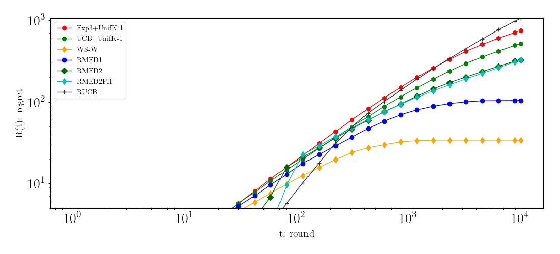
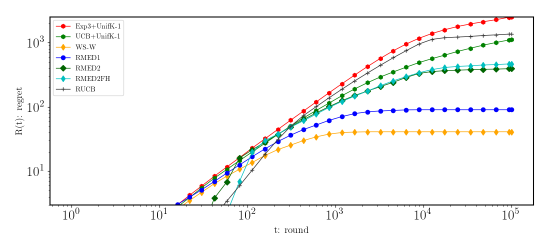
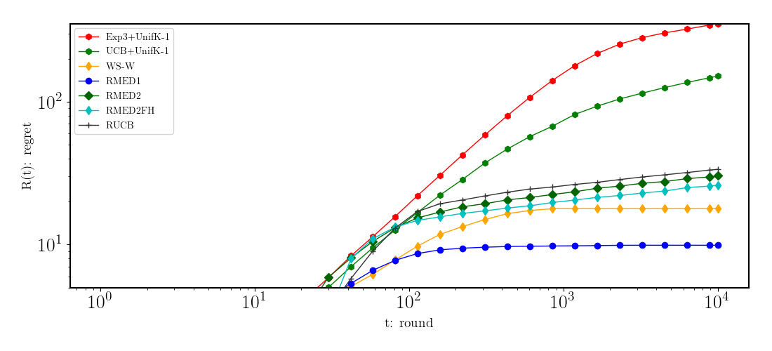
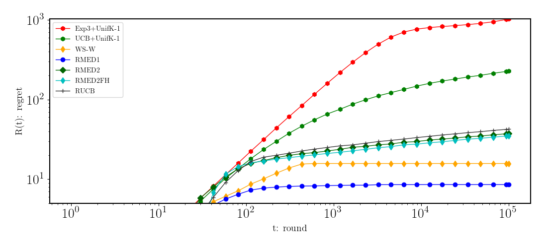
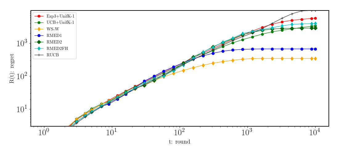
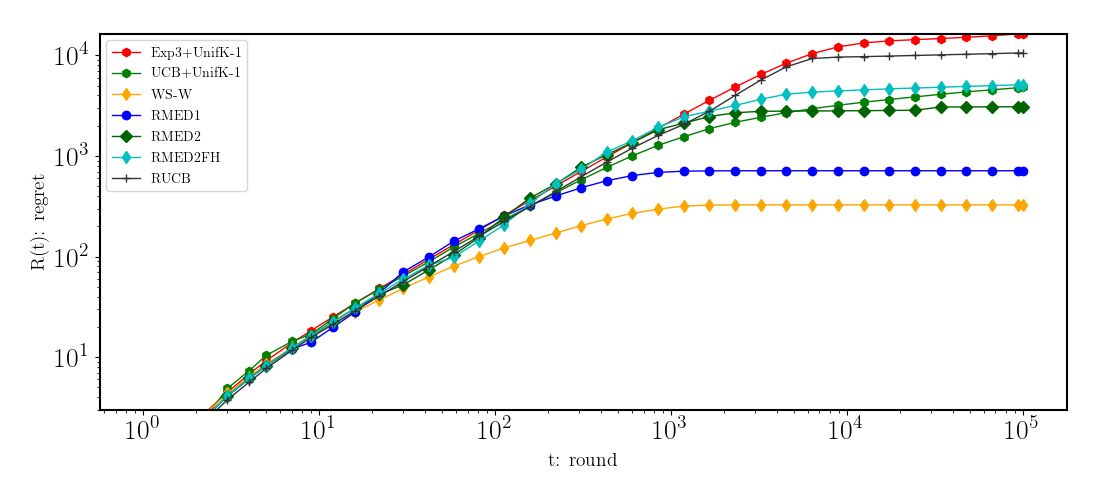
Figure 6.1: Weak regret of Exp3+UnifKminus1 and other algorithms in the stochastic Borda setting with $T=10^{4}$ (left) and $T=10^{5}$ (right) for arXiv (top), cyclic (middle), and sushi (bottom)

6.1.2 Exp3-Sparring, Exp3.P-Sparring, VN+UnifK-1

We would like to show the insufficiency of Exp3-Sparring, Exp3.P-Sparring, and VN+UnifK-1 in the Borda setting. To do so, we generate a sequence of outcomes based on the preference matrix

$$\mathbf{P}=\begin{bmatrix}0.5&1.0&0.55&0.55&0.55\\ 0.0&0.5&1.0&1.0&1.0\\ 0.45&0.0&0.5&0.5&0.5\\ 0.45&0.0&0.5&0.5&0.5\\ 0.45&0.0&0.5&0.5&0.5\end{bmatrix},$$

whose Borda winner is the second action, while its von-Neumann winner has only support by the first action. Let this sequence be denoted by

$$\left(\mathbf{M}^{t}\right)_{t=1}^{T}\text{ with }\mathbf{M}^{t}\sim\mathbf{P}\text{ such that }\frac{1}{T}\sum_{t=1}^{T}\mathbf{M}^{t}=\mathbf{P}.$$ (6.1)

Experiment Setup

Due to $20$ being the smallest positive number guaranteeing integer multiplicity, we construct a sequence of $\tau=20$ outcome matrices matrices $\left(\mathbf{M}^{t}\right)_{t=1}^{\tau}$ the following way: for every sorted pair of actions $(i,j)\subseteq[K]\times[K]$ with $i<j$, we construct a sequence of binary outcomes by considering a random permutation of the multiset with support in $\left\{1,-1\right\}$, with multiplicities $\tau\cdot P_{ij}$ and $\tau\cdot P_{ji}$, respectively. Assuming that $T\equiv 0\pmod{\tau}$, repeating the resulting sequence $\frac{T}{\tau}$ times yields a sequence fulfilling (6.1) by construction. Sequences were generated for $T=10^{3},10^{4},10^{5}$, and the execution of all three algorithms was repeated 100 times, allowing to approximate the mean and standard deviation with respect to the algorithm’s internal randomisation. This experiment can be reproduced by following the steps described in Appendix B.2.

Results

Figure 6.2 depicts the mean cumulative weak regret for all four algorithms. In contrast to Exp3+UnifKminus1, whose weak regret behaves sublinearly in $t$, the weak regret of the other three algorithms grows linearly in $t$, suggesting that they are not suitable for the Borda setting.

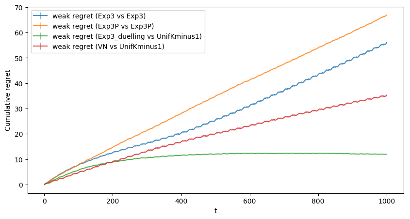
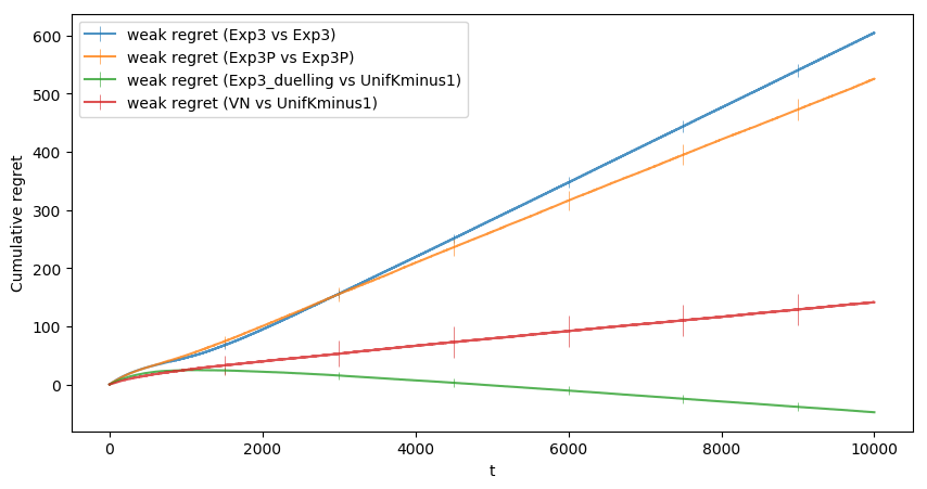
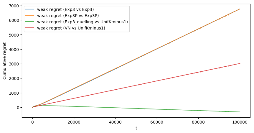
Figure 6.2: Weak Regret of Exp3+UnifKminus1, Exp3-Sparring, Exp3.P-Sparring, and VN+UnifK-1 with $T=10^{3}$ (top-left), $T=10^{4}$ (top-right), and $T=10^{5}$ (bottom) in Borda Setting

6.2 Copeland Regret

The analysis of Exp3+UnifKminus1 in the non-utility-based setting in Section 5.2 was restricted to the loss setting induced by the Borda winner. At the same time, Dudík et al. (2015) claimed that Algorithm 3 suffers sublinear strong regret in the von-Neumann setting. This suggests that these algorithms can suffer linear Copeland regret even in non-adversarial instances, which we show experimentally.

6.2.1 Exp3+UnifKminus1

As Exp3+UnifKminus1 spends on expectation at most $O\left(\sqrt{KT\log K}\right)$ on exploration, the cumulative difference between the Copeland loss incurred by the first action, which is chosen by an instance of the Exp3 algorithm, and the equivalent loss incurred by the Copeland winner can be linear in $t$ if the Borda winner is not identical to the Copeland winner. We will assume the following preference matrix:

$$\mathbf{P}=\begin{bmatrix}0.5&1.0&1.0&0.4&0.4\\ 0.0&0.5&0.6&0.6&0.6\\ 0.0&0.4&0.5&0.4&0.6\\ 0.6&0.4&0.6&0.5&0.4\\ 0.6&0.4&0.4&0.6&0.5\end{bmatrix}.$$

Given a sequence

$$\left(\mathbf{M}^{t}\right)_{t=1}^{T}\text{ with }\mathbf{M}^{t}\sim\mathbf{P}\text{ such that }\frac{1}{T}\sum_{t=1}^{T}\mathbf{M}^{t}=\mathbf{P},$$

the latter assumption implying that, almost surely, the first action is constitutes the unique Borda winner, while the Copeland winner has only support by the second action. The cumulative Borda loss and Copeland loss vectors, in expectation, are given by

$$\mathbb{E}\left[\mathbf{L}_{B}\right] =\frac{T}{K}\begin{bmatrix}1.7&2.7&3.1&2.5&2.5\end{bmatrix}^{T}$$

$$\mathbb{E}\left[\mathbf{L}_{C}\right] =\frac{T}{K-1}\begin{bmatrix}2&1&3&2&2\end{bmatrix}^{T}.$$

This implies that, on expectation, the Borda winner suffers Copeland loss $\frac{2}{K-1}$ every round, while sampling an action from the remaining arms uniformly at random suffers Copeland loss $\frac{2}{K-1}$ as well. This implies that Exp3+UnifKminus1 suffers at most $\frac{1}{K-1}\left(\frac{1}{4}\cdot 1+\frac{3}{4}\cdot 2-1\right)=\frac{3}{16}$ instantaneous weak regret in expectation whenever it selects the Borda winner as first action. As we are not interested in upper bounding the expected regret, we will resort to experimental verification.

Experiment Setup

The experiment setup is similar to the one described in 6.1.2, with $\tau=10$, and $T=10^{3},10^{4}$. The execution of Exp3+UnifKminus1 was repeated 100 times, to obtain a better estimate of the expected regret with respect to the algorithm’s internal randomisation. This experiment can be reproduced by following the steps described in Appendix B.3.

Results

Figure 6.3 depicts the mean weak regret accumulated over time for the two experiments, which grows linearly in $t$ with very little variance. This supports our claim that Exp3+UnifKminus1 is not suitable in scenarios requiring the minimisation of the Copeland loss, and can be forced to suffer weak regret linear in $t$ if the Copeland winner is not identical to the Borda winner.

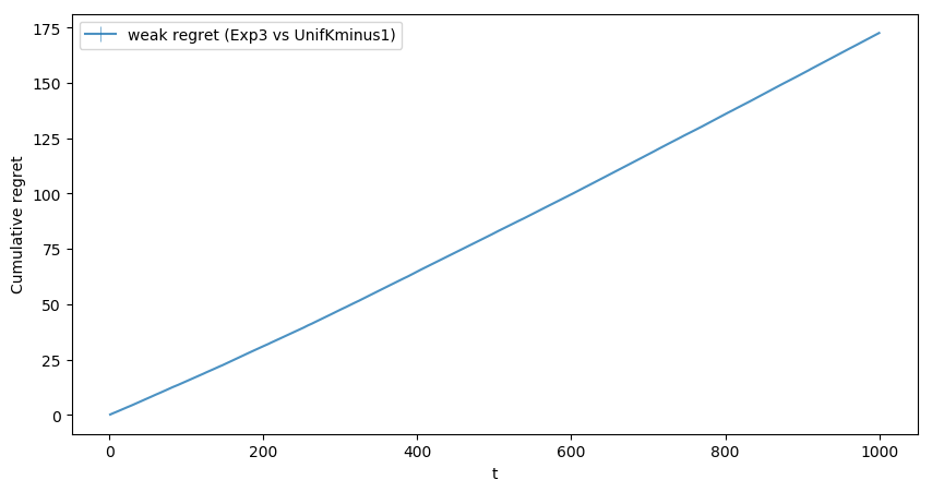
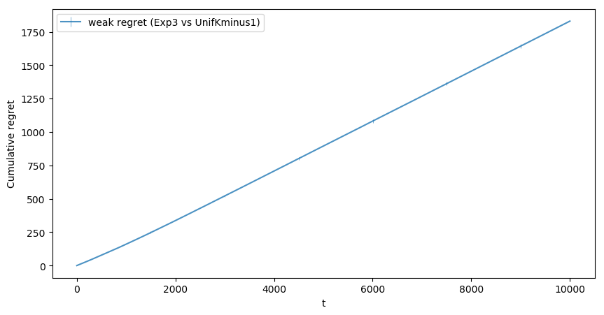
Figure 6.3: Weak Regret of Exp3+UnifKminus1 with $T=1000$ (left) and $T=10000$ (right) in Copeland Setting

6.2.2 Exp3-Sparring, Exp3.P-Sparring, VN+UnifK-1

Unlike VN+UnifK-1, which was specifically designed to approximate the von-Neumann winner, we include Exp3.P-Sparring in this section due to Dudík et al. (2015) claiming the very same. We add Exp3-Sparring for completeness. Assuming that all these focus on finding the von-Neumann winner, we conjecture that they can suffer linear weak regret in the Copeland setting, given that the von-Neumann winner has support by actions which do not constitute the Copeland winner. (Dudík et al., 2015, p.17) used the following preference matrix for illustrating a stochastic non-utility-based case inducing a von-Neumann with no support of the Copeland winner :

$$\mathbf{P}=\begin{bmatrix}0.5&0.75&0.25&0.75&0.025\\ 0.25&0.5&0.75&0.4&0.75\\ 0.75&0.25&0.5&0.4&0.75\\ 0.25&0.6&0.6&0.5&0.75\\ 0.975&0.25&0.25&0.25&0.5\end{bmatrix},$$ (6.2)

which induces a von-Neumann winner which is a uniform distribution over the first three actions $\begin{bmatrix}1/3&1/3&1/3&0&0\end{bmatrix}$, and a Copeland winner focussing on the fourth action (Dudík et al., 2015).

Experiment Setup

The experiment setup is similar to the one described in 6.2.2 with $\tau=40$, and $T=10^{3},10^{4}$. Again, all algorithms were run 100 times. This experiment can be reproduced by following the steps described in Appendix B.4.

Results

Figure 6.4 depicts the mean weak regret of the three algorithms taken into consideration in this experiment. The mean weak regret increases linearly in $t$, confirming our previous claim. In conclusion, none of the algorithms suggested in Chapter 4 are sufficient for the non-utility-based duelling bandit problem in the Copeland setting.

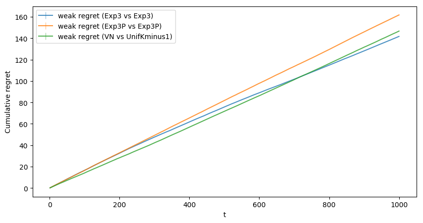
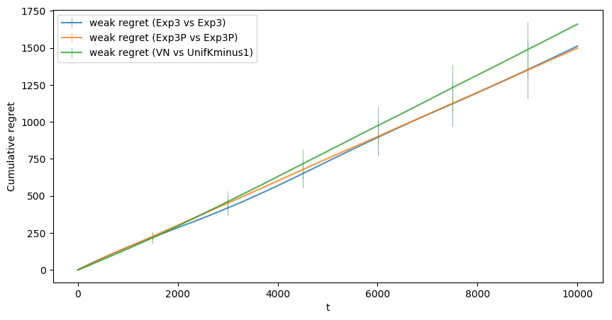
Figure 6.4: Weak Regret of Exp3-Sparring, Exp3.P-Sparring, and VN+UnifK-1 with $T=10^{3}$ (left) and $T=10^{4}$ (right) in Copeland Setting

6.3 Von-Neumann Regret

This section shows that Exp3+UnifKminus1 is not suitable for the von-Neumann setting. The preference matrix (6.1.2) induces a von-Neumann winner which has no support by the Borda winner. However, the uniform exploration behaviour guarantees that in any round, Exp3+UnifKminus1 suffers on expectation at most

$$1-\left(\frac{3}{4}\cdot 0.45+\frac{1}{4}0.5\right)=0.5375$$

instantaneous loss, which is close to the von-Neumann winner’s loss of $0.5$ when considering weak regret. This makes it more difficult to observe high regret in experiments with reasonably small time horizons. For this reason we introduce a larger preference matrix with $K=16$ arms. Based on the preference matrix (6.2), we created a larger matrix with $K=16$ arms, which increases the loss of a uniformly sampled action without modifying the Borda winner or the von-Neumann winner.

$$\mathbf{P}=\begin{bmatrix}0.5&0.75&0.25&1.0&0.025&0.8&\ldots&0.8\\ 0.25&0.5&0.75&1.0&0.75&0.8&\ldots&0.8\\ 0.75&0.25&0.5&1.0&0.75&0.8&\ldots&0.8\\ 0.0&0.0&0.0&0.5&0.75&1.0&\ldots&1.0\\ 0.975&0.25&0.25&0.25&0.5&0.8&\ldots&0.8\\ 0.2&0.2&0.2&0.0&0.2&0.5&\ldots&0.5\\ \vdots&\vdots&\vdots&\vdots&\vdots&\vdots&\ddots&\vdots\\ 0.2&0.2&0.2&0.0&0.2&0.5&\ldots&0.5\\ \end{bmatrix}$$

Similar to the original setting, the von-Neumann winner is $\begin{bmatrix}1/3&1/3&1/3&0&\ldots&0\end{bmatrix}$, while the unique Borda winner is the fourth action.

6.3.1 Experiment Setup

This experiment setup is similar to the one described in Subsection 6.2.2, using $\tau=40$, $T=10^{3},10^{4},10^{5}$, and 10 iterations. This experiment can be reproduced by following the steps described in Appendix B.5.

6.3.2 Results

Figure 6.5 depicts the mean weak regret of the four algorithms taken into consideration in this experiment. The regret of the Exp3-Sparring and VN+UnifK-1 quickly becomes negative. Exp3.P-Sparring has noticeably more exploration, suggesting that the $O\left(\sqrt{KT\log{\frac{K}{\delta}}}\right)$ bound on the expected strong regret, as argued for by Dudík et al. (2015), hides a large constant. The algorithm of interest, Exp3+UnifKminus1, suffers linear regret in this experiment, as its first arm approximates the wrong winner without its second arm compensating for it. This shows that it is not suitable for the von-Neumann setting.

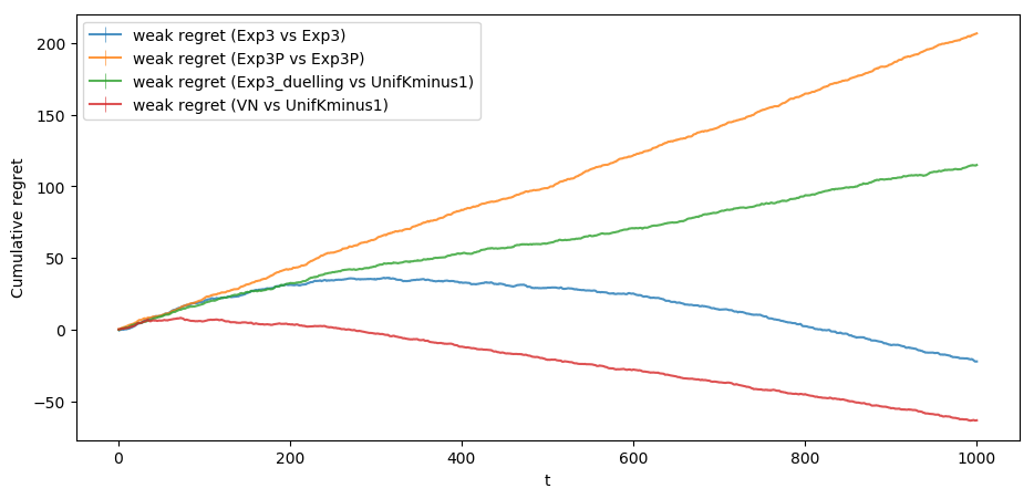
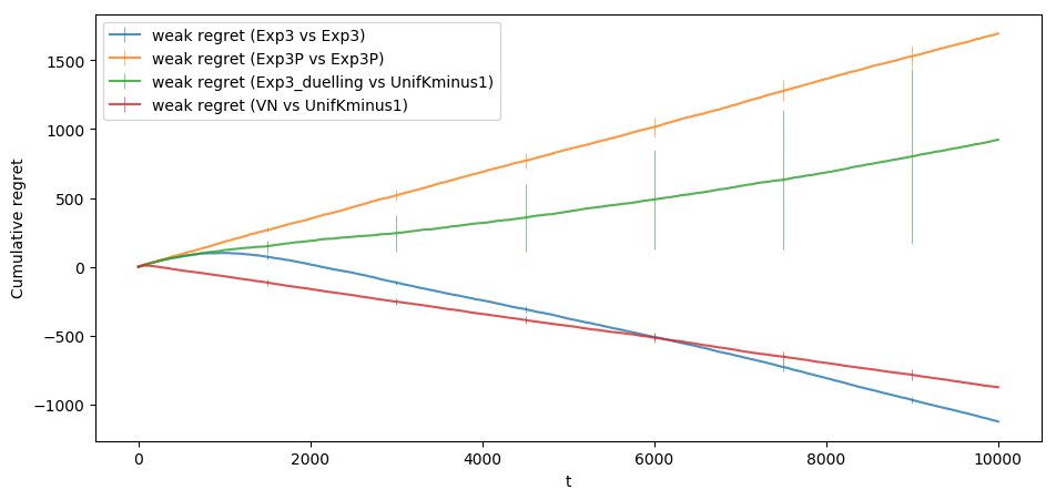
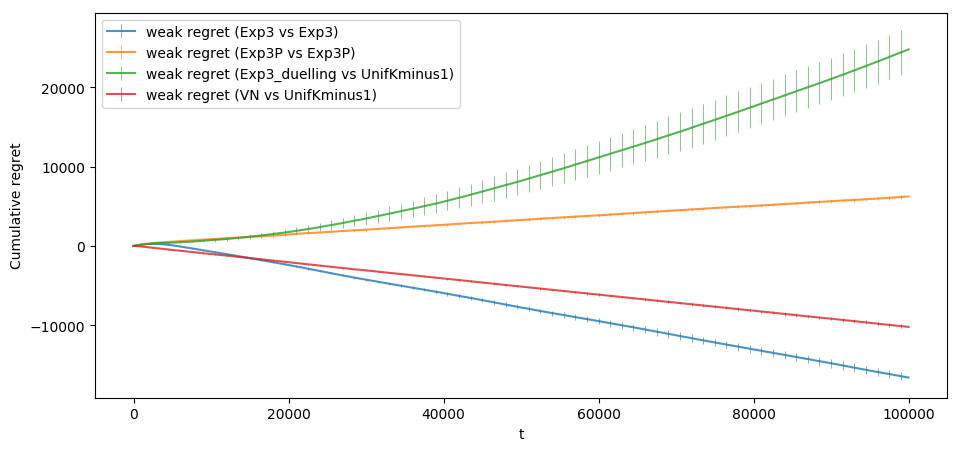
Figure 6.5: Weak Regret of Exp3-Sparring, Exp3.P-Sparring, Exp3+UnifKminus1, and VN+UnifK-1 with $T=10^{3}$ (top-left), $T=10^{5}$ (top-right), and $T=10000$ (bottom-left) in von-Neumann Setting

6.4 Utility-Based Regret

This section compares the empirical performance of Exp3+UnifKminus1 to other algorithms in the stochastic setting. Due to the absence of readily available datasets inducing a linear order, we resort to a small synthetic preference matrix. Again, we restrict ourselves to weak regret, as the expected strong regret of Exp3+UnifKminus1 scales linearly in $T$, while the strong regret is an upper bound on the weak regret.

In addition to our modifications presented in Section 6.1, we implemented REX3 according to (Gajane et al., 2015, Algorithm 1), using $\gamma=\min\left\{\frac{1}{2},\sqrt{\frac{K\log K}{0.5T}}\right\}$.

6.4.1 Experiment Setup

We consider the following preference matrix, which induces a total order:

Arithmetic

As suggested by Komiyama et al. (2015), this preference matrix assumes values $P_{ij}=\frac{1}{2}+\frac{j-i}{20}$ for all $K=8$ actions. This corresponds to a utility vector $\mathbf{x}\in\left[0,1\right]^{K}$ with $x_{i}=1-\frac{i}{10}$ and the linear link function (3.3).

All the simulation parameters are identical to the ones described in Subsection 6.1.1, i.e. $T=10^{4},10^{5}$, we use 100 iterations, and all UCB-based algorithms use $\alpha=0.51$.

6.4.2 Results

Figure 6.6 shows the cumulative weak regret for a range of algorithms. Exp3+UnifKminus1 behaves similarly as in the Borda setting, suffering high regret in comparison to the more specialised algorithms. IF suffers relatively high regret, which is probably because of the small gap in preference between the two best actions. As SAVAGE, REX, and Exp3+UnifKminus1 are generic algorithms, they suffer higher regret than their specialised counterparts RMED and WS-W. UCB+UnifK-1 performs slightly better than REX3 and MultiSBM in our experiments.

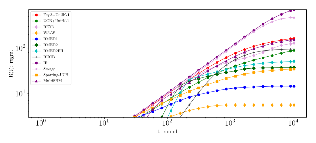
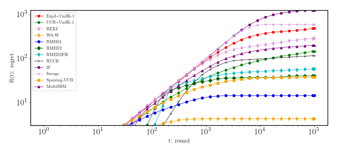
Figure 6.6: Weak regret of Exp3+UnifKminus1 and other algorithms in the stochastic Utility-based setting with $T=10^{4}$ (left) and $T=10^{5}$ (right) for arithmetic

Chapter 7 Discussion

We have presented a duelling bandits algorithm designed for the adversarial setting with the weak regret, effectively reducing the problem to a classical bandit problem as suggested by previous literature (Urvoy et al., 2013; Zoghi et al., 2014; Jamieson et al., 2015). In the course of proving upper bounds on the expected weak regret, we modified the parameterisation, yielding a tighter upper bound in comparison with the standard reduction. These bounds, which are comparable to those of Exp3, hold for both the utility-based setting and the Borda winner setting. The Condorcet setting, the Copeland setting, and the von-Neumann setting can induce a winner which is different from the Borda winner. As demonstrated experimentally, Exp3+UnifKminus1 converges to the wrong action in these scenarios, accumulating regret linear in $T$. While the Condorcet winner is indeed more appropriate than the Borda winner in settings where the set of actions as a whole is less does not directly influence an individual action’s quality (Zoghi et al., 2014), there are scenarios where the Borda winner has the properties of the desired winner. As the concept of the Borda winner is rooted in voting theory, the Borda winner can be used to resolve voting paradoxes when Condorcet-consistency is not required (Chevaleyre et al., 2007). Jamieson et al. (2015) highlights the robustness of the Borda winner to estimation errors in the preference matrix in contrast to the Condorcet winner. The argument of low robustness is also applicable to the more general Copeland winner. In conclusion, the answer to whether the Borda winner is the appropriate modelling criterion depends solely on the application’s problem formulation.

When used in the stochastic setting, Exp3+UnifKminus1 and Exp3 share the same drawback of relatively high regret, as their parameterisations effectively differ only by a multiplicative constant. In case the environment is known to be stochastic, our experiments suggested that replacing the Exp3 algorithm with a UCB-based algorithm can reduce the regret. In the utility-based setting and the more general Condorcet winner setting this modification is not enough to keep up with more specialised algorithms such as WS-W and RMED1, whose expected regret is upper bounded by $O(\log T)$ or even $O(1)$ in the utility-based setting. The Borda setting has only been covered by Jamieson et al. (2015) so far, who make some structural assumptions on the preference matrix, allowing faster convergence to the winner than the standard reduction scheme allows for. Applying algorithms with specific performance guarantees in both the stochastic and the adversarial environment, as presented by Bubeck and Slivkins (2012); Seldin and Slivkins (2014), is left for future work.

For the sake of simplicity, we have assumed that the time horizon $T$ is known to the algorithm, allowing to optimise the choice of parameters. By modifying the analysis, as performed by Bubeck and Cesa-Bianchi (2012), Exp3+UnifKminus1 can be generalised to an anytime algorithm, worsening the bound on the expected regret by a factor of $\sqrt{2}$.

Our theoretical analysis of Exp3+UnifKminus1 relies on the linear link function. Generalisation to other link functions, e.g. the Bradley-Terry model or the probit model, is left for future work.

Overall, Exp3+UnifKminus1 should be not be seen as an algorithm optimised for weak regret, but a generic reduction to the cardinal bandit problem with slightly tuned parameters. Due to its persistent uniform exploration it is not suitable when considering strong regret. It is most suitable for adversarial settings, where it is applicable to both the utility-based setting and the Borda setting.

Appendix A Proof of Lemma 5.1

Proof.

Let $n\in\mathbb{N},f:\mathbb{R}^{n}\to\mathbb{R}$ and

$$f(\mathbf{x}):=-\sum_{i=1}^{n}\sum_{j=1}^{n}(x_{i}-x_{j}+1)^{2}=2\sum_{i=1}^{n}\sum_{j=1}^{n}x_{i}x_{j}-2n\sum_{i=1}^{n}x_{i}^{2}-n^{2}$$

The above problem can be reformulated as constrained convex optimisation problem:

$$\underset{\mathbf{x}\in\mathbb{R}^{n}}{\mathrm{minimise}}\,f(\mathbf{x})\text{ such that }0\leq x_{i}\leq 1\text{ for }i=1,\ldots,n.$$

Using the set of functions

$$g_{i}(\mathbf{x}) =x_{i}-1$$

$$g_{n+i}(\mathbf{x}) =-x_{i},$$

the two-sided inequality constraints can be expressed as

$$g_{i}\leq 0\text{ for }i=1,\ldots,2n,$$

yielding the following Lagrangian:

$$L(\mathbf{x},\mathbf{\lambda}) =f(\mathbf{x})+\sum_{i=1}^{2n}\lambda_{i}g_{i}(\mathbf{x})$$

$$=f(\mathbf{x})+\sum_{i=1}^{n}\mathbf{\lambda}_{i}(x_{i}-1)-\sum_{i=1}^{n}\lambda_{n+i}x_{i}.$$

By complementary slackness, the solution $\mathbf{x}^{*},\mathbf{\lambda}^{*}$ satisfies

$$\lambda_{i}^{*}(x_{i}^{*}-1)=\lambda_{n+i}^{*}x_{i}^{*}=0$$ (A.1)

for all $i=1,\ldots,n$. Let $S_{0}=\left\{i\middle|x_{i}=0\right\},S_{1}=\left\{i\middle|x_{i}=1\right\},S_{\lambda}=\left\{i\middle|0<x_{i}<1\right\}$ and $n_{0}=\left\lvert S_{0}\right\rvert,n_{1}=\left\lvert S_{1}\right\rvert,n_{\lambda}=\left\lvert S_{\lambda}\right\rvert$. By (A.1),

$$\forall i\in S_{\lambda}:\lambda_{i}^{*}=\lambda_{n+i}^{i}=0.$$

This simplifies the Lagrangian condition for all $i\in S_{\lambda}$ to

$$\frac{\partial L(\mathbf{x}^{*},\mathbf{\lambda}^{*})}{\partial x_{i}}=\frac{\partial f(\mathbf{x}^{*})}{\partial x_{i}}=0,$$

which is equivalent to

$$\frac{\partial f(\mathbf{x}^{*})}{\partial x_{i}}=4\sum_{j=1,j\neq i}^{n}x_{j}+4x_{i}-4nx_{i}=0.$$

Its solution is given by

$$x_{i}=\frac{1}{n-1}\sum_{j=1,j\neq i}^{n}x_{j}.$$

As

$$\sum_{j=1,j\neq i}^{n}x_{j} =0n_{0}+1n_{1}+(n_{\lambda}-1)x_{i}$$

$$=n_{1}+(n_{\lambda}-1)x_{i},$$

it follows that

$$x_{i} =\frac{n_{1}}{(n-1)\left(1-\frac{n_{\lambda}-1}{n-1}\right)}$$

$$=\frac{n_{1}}{n-n_{\lambda}}$$

$$=\frac{n_{1}}{n_{0}+n_{1}}.$$

As $x_{i}\in[0,1]$, $n_{0}+n_{1}>0$. We can rewrite the original optimisation problem as integer linear programme

$$\underset{n_{0},n_{1},n_{\lambda}}{\mathrm{maximise}}\, n^{2}+2n_{0}n_{1}+2n_{0}n_{\lambda}\left(\frac{n_{1}}{n_{0}+n_{1}}\right)^{2}+2n_{1}n_{\lambda}\left(\frac{n_{0}}{n_{0}+n_{1}}\right)^{2}$$

$$=n^{2}+2n_{0}n_{1}\left(1+\frac{(n-(n_{0}+n_{1}))(n_{0}+n_{1})}{(n_{0}+n_{1})^{2}}\right)$$

$$=n^{2}+\frac{2n_{0}n_{1}n}{n_{0}+n_{1}},$$

such that $n_{0},n_{1},n_{\lambda}\in\mathbb{N}_{0},n_{0}+n_{1}+n_{\lambda}=n,n_{0}+n_{1}>0$. By relaxing the last constraint with $n_{0}+n_{1}\leq n$, the initial problem can be relaxed to the corresponding real-valued version

$$n^{2}+\frac{2n_{0}n_{1}n}{n_{0}+n_{1}}\leq\frac{3n^{2}}{2},$$

which is equivalent to

$$\frac{4n_{0}n_{1}}{n_{0}+n_{1}}\leq n.$$ (A.2)

We will now show that

$$\frac{4n_{0}n_{1}}{n_{0}+n_{1}}\leq n_{0}+n_{1}.$$ (A.3)

As $n_{0}+n_{1}>0$, this inequality can be rearranged to

$$4n_{0}n_{1}\leq(n_{0}+n_{1})^{2},$$

which is equivalent to

$$0\leq(n_{0}-n_{1})^{2},$$

proving (A.3), which in turn proves (A.2), as $n_{0}+n_{1}\leq n$. ∎

Appendix B Experiments

This appendix contains the scripts used to automate the experiments, facilitating the reproduction of our results.

B.1 Exp3+UnifKminus1 in the Stochastic Borda Setting

Listing 1: Experiment Setup for 1 Exp3+UnifKminus1 in the Stochastic Borda Setting

⬇

#!/usr/bin/bash

set -e

base_filename="borda_stochastic_%s_%d"

git checkout borda

./compile

mkdir -p out plots

for pref in cyclic arxiv sushi; do

for T in 10000 100000; do

result_file="$(printf $base_filename.txt $pref $T)"

plot_file="$(printf plots/$base_filename.png $pref $T)"

build/main -r 100 -t "$T" -i prefmats/pref_${pref}.txt \

-o "$result_file"

python2 simpleplot.py "out/$result_file" "$plot_file"

done

done

B.2 Exp3+UnifKminus1, Exp3-Sparring, Exp3.P-Sparring, VN+UnifK-1 in the Borda Setting

Listing 2: Experiment Setup for 1 Exp3+UnifKminus1, 2 Exp3-Sparring, 3 Exp3.P-Sparring, 4 VN+UnifK-1 in the Borda Setting

⬇

#!/usr/bin/bash

base_filename="borda_vn_%d"

for rep in 50 500 5000; do

T=$((rep * 20))

seq_file="$(printf seq/$base_filename.xz $T)"

result_file="$(printf results/$base_filename.xz $T)"

plot_dir="$(printf plots/$base_filename $T)"

./gen_seq.py -o "$seq_file" -T 20 --rep "$rep" \

--type gen_from_preference_matrix_rep -P prefs/borda_vonneumann

./run_simulation.py -i "$seq_file" --niter 100 -o "$result_file" \

--algos Exp3+Exp3 Exp3P+Exp3P Exp3_duelling+UnifKminus1 VN+UnifKminus1

./plot_results.py -W Borda -i "$result_file" -o "$plot_dir"

done

B.3 Exp3+UnifKminus1 in Copeland Setting

Listing 3: Experiment Setup for 1 Exp3+UnifKminus1 in Copeland Setting

⬇

#!/usr/bin/bash

base_filename="copeland_exp3_unifkminus1_%d"

for rep in 100 1000; do

T=$((rep * 10))

seq_file="$(printf seq/$base_filename.xz $T)"

result_file="$(printf results/$base_filename.xz $T)"

plot_dir="$(printf plots/$base_filename $T)"

./gen_seq.py -o "$seq_file" -T 10 --rep "$rep" \

--type gen_from_preference_matrix_rep -P prefs/copeland_borda

./run_simulation.py -i "$seq_file" --niter 100 -o "$result_file" \

--algos Exp3+UnifKminus1

./plot_results.py -W Copeland -i "$result_file" -o "$plot_dir"

done

B.4 Exp3-Sparring, Exp3.P-Sparring, VN+UnifK-1 in Copeland Setting

Listing 4: Experiment Setup for 2 Exp3-Sparring, 3 Exp3.P-Sparring, 4 VN+UnifK-1 in Copeland Setting

⬇

#!/usr/bin/bash

base_filename="copeland_vn_%d"

for rep in 25 250; do

T=$((rep * 40))

seq_file="$(printf seq/$base_filename.xz $T)"

result_file="$(printf results/$base_filename.xz $T)"

plot_dir="$(printf plots/$base_filename $T)"

./gen_seq.py -o "$seq_file" -T 40 --rep "$rep" \

--type gen_from_preference_matrix_rep -P prefs/copeland_vonneumann

./run_simulation.py -i "$seq_file" --niter 100 -o "$result_file" \

--algos Exp3+Exp3 Exp3P+Exp3P VN+UnifKminus1

./plot_results.py -W Copeland -i "$result_file" -o "$plot_dir"

done

B.5 Exp3+UnifKminus1 in Von-Neumann Setting

Listing 5: Experiment Setup for 1 Exp3+UnifKminus1 in Von-Neumann Setting

⬇

#!/usr/bin/bash

base_filename="vn_%d"

for rep in 25 250 2500; do

T=$((rep * 40))

seq_file="$(printf seq/$base_filename.xz $T)"

result_file="$(printf results/$base_filename.xz $T)"

plot_dir="$(printf plots/$base_filename $T)"

./gen_seq.py -o "$seq_file" -T 40 --rep "$rep" \

--type gen_from_preference_matrix_rep -P prefs/different_winners

./run_simulation.py -i "$seq_file" --niter 100 -o "$result_file" \

--algos Exp3+Exp3 Exp3P+Exp3P Exp3_duelling+UnifKminus1 VN+UnifKminus1

./plot_results.py -W von-Neumann -i "$result_file" -o "$plot_dir"

done

B.6 Exp3+UnifKminus1 in Stochastic Utility-based Setting

Listing 6: Experiment Setup for 1 Exp3+UnifKminus1 in Stochastic Utility-based Setting

⬇

#!/usr/bin/bash

set -e

base_filename="utility_stochastic_%s_%d"

git checkout utility

./compile

mkdir -p out plots

for pref in arithmetic; do

for T in 10000 100000; do

result_file="$(printf $base_filename.txt $pref $T)"

plot_file="$(printf plots/$base_filename.png $pref $T)"

build/main -r 100 -t "$T" -i prefmats/pref_${pref}.txt \

-o "$result_file"

python2 simpleplot.py "out/$result_file" "$plot_file"

done

done

References

- Ailon et al. (2014) Nir Ailon, Zohar Karnin, and Thorsten Joachims. Reducing dueling bandits to cardinal bandits. In Proceedings of the 31st International Conference on International Conference on Machine Learning - Volume 32, ICML’14, pages II–856–II–864. JMLR.org, 2014. URL http://dl.acm.org/citation.cfm?id=3044805.3044988.
- Auer et al. (2002) Peter Auer, Nicolò Cesa-Bianchi, and Paul Fischer. Finite-time analysis of the multiarmed bandit problem. Mach. Learn., 47(2-3):235–256, May 2002. ISSN 0885-6125. doi: 10.1023/A:1013689704352. URL https://doi.org/10.1023/A:1013689704352.
- Auer et al. (2003) Peter Auer, Nicolò Cesa-Bianchi, Yoav Freund, and Robert E. Schapire. The nonstochastic multiarmed bandit problem. SIAM J. Comput., 32(1):48–77, January 2003. ISSN 0097-5397. doi: 10.1137/S0097539701398375. URL https://doi.org/10.1137/S0097539701398375.