Non-local U-Nets for Biomedical Image Segmentation

Abstract

Deep learning has shown its great promise in various biomedical image segmentation tasks. Existing models are typically based on U-Net and rely on an encoder-decoder architecture with stacked local operators to aggregate long-range information gradually. However, only using the local operators limits the efficiency and effectiveness. In this work, we propose the non-local U-Nets, which are equipped with flexible global aggregation blocks, for biomedical image segmentation. These blocks can be inserted into U-Net as size-preserving processes, as well as down-sampling and up-sampling layers. We perform thorough experiments on the 3D multimodality isointense infant brain MR image segmentation task to evaluate the non-local U-Nets. Results show that our proposed models achieve top performances with fewer parameters and faster computation.

Introduction

In recent years, deep learning methods, such as fully convolutional networks (FCN) (?), U-Net (?), Deeplab (?; ?), and RefineNet (?), have continuously set performance records on image segmentation tasks. In particular, U-Net has served as the backbone network for biomedical image segmentation. Basically, U-Net is composed of a down-sampling encoder and an up-sampling decoder, along with skip connections between them. It incorporates both local and global contextual information through the encoding-decoding process.

Many variants of U-Net have been developed and they achieved improved performance on biomedical image segmentation tasks. For example, residual deconvolutional network (?) and residual symmetric U-Net (?) addressed the 2D electron microscopy image segmentation task by building a U-Net based network with additional short-range residual connections (?). In addition, U-Net was extended from 2D to 3D cases for volumetric biomedical images, leading to models like 3D U-Net (?), V-Net (?), and convolution-concatenate 3D-FCN (CC-3D-FCN) (?).

Despite the success of these studies, we conduct an in-depth study of U-Net based models and observe two limitations shared by them. First, the encoder usually stacks size-preserving convolutional layers, interlaced with down-sampling operators, to gradually reduce the spatial sizes of feature maps. Both convolutions and down-sampling operators are typically local operators, which apply small kernels to scan inputs and extract local information. Stacking them in a cascade way results in large effective kernels and is able to aggregate long-range information. As the biomedical image segmentation usually benefits from a wide range of contextual information, most prior models have a deep encoder, i.e., an encoder with many stacked local operators. It hurts the efficiency of these models by introducing a considerably large amount of training parameters, especially when more down-sampling operators are employed, since the number of feature maps usually gets doubled after each down-sampling operation. In addition, more down-sampling operators cause the loss of more spatial information during encoding, which is crucial for biomedical image segmentation. Second, the decoder is built in a similar way to the encoder, by replacing down-sampling operators with up-sampling operators. Popular up-sampling operators, like deconvolutions and unpooling layers, are local operators as well (?). However, the up-sampling process involves the recovery of spatial information, which is hard without taking global information into consideration. To conclude, it will improve both the effectiveness and efficiency of U-Net based models to develop a new operator capable of performing non-local information aggregation. As U-Net has size-preserving processes, as well as down-sampling and up-sampling layers, the new operator is supposed to be flexible to fit these cases.

In this work, we address the two limitations and propose the non-local U-Nets for biomedical image segmentation. To address the first limitation above, we propose a global aggregation block based on the self-attention operator (?; ?; ?), which is able to aggregate global information without a deep encoder. This block is further extended to an up-sampling global aggregation block, which can alleviate the second problem. To the best of our knowledge, we are the first to make this extension. We explore the applications of these flexible global aggregation blocks in U-Net on the 3D multimodality isointense infant brain magnetic resonance (MR) image segmentation task. Experimental results show that our proposed non-local U-Nets are able to achieve the top performance with fewer parameters and faster computation.

Non-local U-Net

In this section, we introduce our proposed non-local U-Nets. We first illustrate the specific U-Net framework used by our models. Based on the framework, our models are composed of different size-preserving, down-sampling and up-sampling blocks. We describe each block and propose our global aggregation blocks to build the non-local U-Nets.

U-Net Framework

We describe the non-local U-Nets in 3D cases. Lower or higher dimensional cases can be easily derived. An illustration of the basic U-Net framework is given in Fig. 1. The input first goes through an encoding input block, which extracts low-level features. Two down-sampling blocks are used to reduce the spatial sizes and obtain high-level features. Note that the number of channels is doubled after each down-sampling block. A bottom block then aggregates global information and produces the output of the encoder. Correspondingly, the decoder uses two up-sampling blocks to recover the spatial sizes for the segmentation output. The number of feature maps is halved after an up-sampling operation.

To assist the decoding process, skip connections copy feature maps from the encoder to the decoder. Differently, in the non-local U-Nets, the copied feature maps are combined with decoding feature maps through summation, instead of concatenation used in U-Net (?; ?). The intuitive way to combine features from the encoder and the decoder is concatenation, providing two sources of inputs to the up-sampling operation. Using summation instead has two advantages (?). First, summation does not increase the number of feature maps, thus reducing the number of trainable parameters in the following layer. Second, skip connections with summation can be considered as long-range residual connections, which are known to be capable of facilitating the training of models.

Given the output of the decoder, the output block produces the segmentation probability map. Specifically, for each voxel, the probabilities that it belongs to each segmentation class are provided, respectively. The final segmentation map can be obtained through a single argmax operation on this probability map. The details of each block are introduced in following sections.

Figure 1: An illustration of the U-Net framework employed by our proposed non-local U-Nets. In this example, the inputs have 2 channels and the segmentation task has 4 classes.

Figure 2: An illustration of the residual blocks employed by our proposed non-local U-Nets. Details are provided in Section “Residual Block”.

Residual Blocks

Residual connections have been shown to facilitate the training of deep learning models and achieve better performance (?). Note that skip connections with summation in our U-Net framework are equivalent to long-range residual connections. To further improve U-Net, the studies in (?; ?; ?) proposed to add short-range residual connections as well. However, those studies did not apply residual connections for down-sampling and up-sampling blocks. Down-sampling block with residual connections has been explored in ResNet (?). We explore the idea for up-sampling blocks based on our proposed up-sampling global aggregation block, as discussed in next section.

In our proposed model, four different residual blocks are used to form a fully residual network, as shown in Fig. 2. Notably, all of them apply the pre-activation pattern (?). Fig. 2(a) shows a regular residual block with two consecutive convolutional layers. Here, batch normalization (?) with the ReLU6 activation function is used before each convolutional layer. This block is used as the input block in our framework. The output block is constructed by this block followed by a $1\times 1\times 1$ convolution with a stride of 1. Moreover, after the summation of skip connections, we insert one such block. Fig. 2(b) is a down-sampling residual block. A $1\times 1\times 1$ convolution with a stride of 2 is used to replace the identity residual connection, in order to adjust the spatial sizes of feature maps accordingly. We employ this block as the down-sampling blocks. Fig. 2(c) illustrates our bottom block. Basically, a residual connection is applied on the proposed global aggregation block. The up-sampling residual block is provided in Fig. 2(d). Similar to the down-sampling block in Fig. 2(b), the identity residual connection is replaced by a $3\times 3\times 3$ deconvolution with a stride of 2 and the other branch is the up-sampling global aggregation block. Our model uses this block as the up-sampling blocks.

Global Aggregation Block

To achieve global information fusion through a block, each position of the output feature maps should depend on all positions of the input feature maps. Such an operation is opposite to local operations like convolutions and deconvolutions, where each output location has a local receptive field on the input. In fact, a fully-connected layer has this global property. However, it is prone to over-fitting and does not work well in practice. We note that the self-attention block used in the Transformer (?) computes outputs at one position by attending to every position of the input. Later, the study in (?) proposed non-local neural networks for video classification, which employed a similar block. While both studies applied self-attention blocks with the aim of capturing long-term dependencies in sequences, we point out that global information of image feature maps can be aggregated through self-attention blocks.

Based on this insight, we propose the global aggregation block, which is able to fuse global information from feature maps of any size. We further generalize it to handle down-sampling and up-sampling, making it a block that can be used anywhere in deep learning models.

Let $X$ represent the input to the global aggregation block and $Y$ represent the output. For simplicity, we use $Conv\_1_{N}$ to denote a $1\times 1\times 1$ convolution with a stride of 1 and $N$ output channels. Note that $Conv\_1_{N}$ does not change the spatial size. The first step of the proposed block is to generate the query ($Q$), key ($K$) and value ($V$) matrices (?), given by

$$Q = Unfold(QueryTransform_{C_{K}}(X)),$$

$$K = Unfold(Conv\_1_{C_{K}}(X)),$$

$$V = Unfold(Conv\_1_{C_{V}}(X)),$$ (1)

where $Unfold(\cdot)$ unfolds a $D\times H\times W\times C$ tensor into a $(D\times H\times W)\times C$ matrix, $QueryTransform_{C_{K}}(\cdot)$ can be any operation that produces $C_{K}$ feature maps, and $C_{K},C_{V}$ are hyper-parameters representing the dimensions of the keys and values. Suppose the size of $X$ is $D\times H\times W\times C$. Then the dimensions of $K$ and $V$ are $(D\times H\times W)\times C_{K}$ and $(D\times H\times W)\times C_{V}$, respectively. The dimension of $Q$, however, is $(D_{Q}\times H_{Q}\times W_{Q})\times C_{K}$, where $D_{Q},H_{Q},W_{Q}$ depend on $QueryTransform(\cdot)$. The left part of Fig. 3 illustrates this step. Here, a $D\times H\times W\times C$ tensor is represented by a $D\times H\times W$ cube, whose voxels correspond to $C$-dimensional vectors.

Figure 3: An illustration of our proposed global aggregation block. Note that the spatial size of the output is determined by that of the query (Q) matrix.

Each row of the $Q$, $K$ and $V$ matrices denotes a query vector, a key vector and a value vector, respectively. Note that the query vector has the same dimension as the key vector. Meanwhile, the number of key vectors is the same as that of value vectors, which indicates a one-to-one correspondence. In the second step, the attention mechanism is applied on $Q$, $K$ and $V$ (?), defined as

$$A = Softmax(\frac{QK^{T}}{\sqrt{C_{K}}}),$$

$$O = AV,$$ (2)

where the dimension of the attention weight matrix $A$ is $(D_{Q}\times H_{Q}\times W_{Q})\times(D\times H\times W)$ and the dimension of the output matrix $O$ is $(D_{Q}\times H_{Q}\times W_{Q})\times C_{V}$. To see how it works, we take one query vector from $Q$ as an example. In the attention mechanism, the query vector interacts with all key vectors, where the dot-product between the query vector and one key vector produces a scalar weight for the corresponding value vector. The output of the query vector is a weighted sum of all value vectors, where the weights are normalized through $Softmax$. This process is repeated for all query vectors and generates $(D_{Q}\times H_{Q}\times W_{Q})$ $C_{V}$-dimensional vectors. This step is illustrated in the box of Fig. 3. Note that Dropout (?) can be applied on $A$ to avoid over-fitting. As shown in Fig. 3, the final step of the block computes $Y$ by

$$Y=Conv\_1_{C_{O}}(Fold(O)),$$ (3)

where $Fold(\cdot)$ is the reverse operation of $Unfold(\cdot)$ and $C_{O}$ is a hyper-parameter representing the dimension of the outputs. As a result, the size of $Y$ is $D_{Q}\times H_{Q}\times W_{Q}\times C_{O}$.

In particular, it is worth noting that the spatial size of $Y$ is determined by that of the Q matrix, i.e., by the $QueryTransform_{C_{K}}(\cdot)$ function in (Global Aggregation Block). Therefore, with appropriate $QueryTransform_{C_{K}}(\cdot)$ functions, the global aggregation block can be flexibly used for size-preserving, down-sampling and up-sampling processes. In our proposed non-local U-Nets, we set $C_{K}=C_{V}=C_{O}$ and explore two different $QueryTransform_{C_{K}}(\cdot)$ functions. For the global aggregation block in Fig. 2(c), $QueryTransform_{C_{K}}(\cdot)$ is $Conv\_1_{C_{K}}$. For the up-sampling global aggregation block in Fig. 2(d), $QueryTransform_{C_{K}}(\cdot)$ is a $3\times 3\times 3$ deconvolution with a stride of 2. The use of this block alleviates the problem that the up-sampling through a single deconvolution loses information. By taking global information into consideration, the up-sampling block is able to recover more accurate details.

Results and Discussion

We perform experiments on the 3D multimodality isointense infant brain MR image segmentation task to evaluate our non-local U-Nets. The task is to perform automatic segmentation of MR images into cerebrospinal fluid (CSF), gray matter (GM) and white matter (WM) regions. We first introduce the baseline model and the evaluation methods used in our experiments. Then the training and inference processes are described. We provide comparison results in terms of both effectiveness and efficiency, and conduct ablation studies to demonstrate that how each global aggregation block in our non-local U-Nets improves the performance. In addition, we explore the trade-off between the inference speed and accuracy based on different overlapping step sizes, and analyze the impact of patch size. The experimental code and dataset information have been made publicly available .

Experimental Setup

We use CC-3D-FCN (?) as our baseline. CC-3D-FCN is a 3D fully convolutional network (3D-FCN) with convolution and concatenate (CC) skip connections, which is designed for 3D multimodality isointense infant brain image segmentation. It has been shown to outperform traditional machine learning methods, such as FMRIB’s automated segmentation tool (FAST) (?), majority voting (MV), random forest (RF) (?) and random forest with auto-context model (LINKS) (?). Moreover, studies in (?) has showed the superiority of CC-3D-FCN to previous deep learning models, like 2D, 3D CNNs (?), DeepMedic (?), and the original 3D U-Net (?). Therefore, it is appropriate to use CC-3D-FCN as the baseline of our experiments. Note that our dataset is different from that in (?).

In our experiments, we employ the Dice ratio (DR) and propose the 3D modified Hausdorff distance (3D-MHD) as the evaluation metrics. These two methods evaluate the accuracy only for binary segmentation tasks, so it is required to transform the 4-class segmentation map predicted by our model into 4 binary segmentation maps for evaluation. That is, a 3D binary segmentation map should be constructed for each class, where 1 denotes the voxel in the position belongs to the class and 0 means the opposite. In our experiments, we derive binary segmentation maps directly from 4-class segmentation maps. The evaluation is performed on binary segmentation maps for CSF, GM and WM.

Specifically, let $P$ and $L$ represent the predicted binary segmentation map for one class and the corresponding ground truth label, respectively. The DR is given by $DR=2|P\cap L|/(|P|+|L|)$, where $|\cdot|$ denotes the number of 1’s in a segmentation map and $|P\cap L|$ means the number of 1’s shared by $P$ and $L$. Apparently, DR is a value in $[0,1]$ and a larger DR indicates a more accurate segmentation.

Table 1: Comparison of segmentation performance between our proposed model and the baseline model in terms of DR. The leave-one-subject-out cross-validation is used. Larger values indicate better performance.

Model	CSF	GM	WM	Average
Baseline	0.9250$\pm$0.0118	0.9084$\pm$0.0056	0.8926$\pm$0.0119	0.9087$\pm$0.0066
Non-local U-Net	0.9530$\pm$0.0074	0.9245$\pm$0.0049	0.9102$\pm$0.0101	0.9292$\pm$0.0050

Table 2: Comparison of segmentation performance between our proposed model and the baseline model in terms of 3D-MHD. The leave-one-subject-out cross-validation is used. Smaller values indicate better performance. Note that 3D-MHD gives different results from MHD.

Model	CSF	GM	WM	Average
Baseline	0.3417$\pm$0.0245	0.6537$\pm$0.0483	0.4817$\pm$0.0454	0.4924$\pm$0.0345
Non-local U-Net	0.2554$\pm$0.0207	0.5950$\pm$0.0428	0.4454$\pm$0.0040	0.4319$\pm$0.0313

Table 3: Comparison of segmentation performance on the 13 testing subjects of iSeg-2017 between our proposed model and the baseline model in terms of DR. Larger values indicate better performance.

Model	CSF	GM	WM
Baseline	0.9324$\pm$0.0067	0.9146$\pm$0.0074	0.8974$\pm$0.0123
Non-local U-Net	0.9557$\pm$0.0060	0.9219$\pm$0.0089	0.9044$\pm$0.0153

The modified Hausdorff distance (MHD) (?) is designed to compute the similarity between two objects. Here, an object is a set of points where a point is represented by a vector. Specifically, given two sets of vectors $A$ and $B$, MHD is computed by $MHD=\max(d(A,B),d(B,A))$, where the distance between two sets is defined as $d(A,B)=1/|A|\sum_{a\in A}{d(a,B)}$, and the distance between a vector and a set is defined as $d(a,B)=\min_{b\in B}||a-b||$. Previous studies (?; ?; ?) applied MHD for evaluation by treating a 3D $D\times H\times W$ map as $H\times W$ $D$-dimensional vectors. However, there are two more different ways to vectorize the 3D map, depending on the direction of forming vectors, i.e., $D\times H$ $W$-dimensional vectors and $D\times W$ $H$-dimensional vectors. Each vectorization leads to different evaluation results by MHD. To make it a direction-independent evaluation metric as DR, we define 3D-MHD, which computes the averaged MHD based on the three different vectorizations. A smaller 3D-MHD indicates a higher segmentation accuracy.

Training and Inference Strategies

Our proposed non-local U-Nets apply Dropout (?) with a rate of 0.5 in each global aggregation block and the output block before the final $1\times 1\times 1$ convolution. A weight decay (?) with a rate of $2e-6$ is also employed. To train the model, we use randomly cropped small patches. In this way, we obtain sufficient training data and the requirement on memory is reduced. No extra data augmentation is needed. The experimental results below suggest that patches with a size of $32^{3}$ leads to the best performance. The batch size is set to 5. The Adam optimizer (?) with a learning rate of 0.001 is employed to perform the gradient descent algorithm.

In the inference process, following (?), we extract patches with the same size as that used in training. For example, to generate $32^{3}$ patches for inference, we slide a window of size $32^{3}$ through the original image with a constant overlapping step size. The overlapping step size must be smaller than or equal to the patch size, in order to guarantee that extracted patches cover the whole image. Consequently, prediction for all these patches provides segmentation probability results for every voxel in the original image. For voxels that receive multiple results due to overlapping, we average them to produce the final prediction. The overlapping step size is an important hyper-parameter affecting the inference speed and the segmentation accuracy. A smaller overlapping step size results in better accuracy, but increases the inference time as more patches are generated. We explore the trade-off in our experiments.

Comparison with the Baseline

We compare our non-local U-Nets with the baseline on our dataset. Following (?), the patch size is set to $32^{3}$ and the overlapping step size for inference is set to $8$. To remove the bias of different subjects, the leave-one-subject-out cross-validation is used for evaluating segmentation performance. That is, for 10 subjects in our dataset, we train and evaluate models 10 times correspondingly. Each time one of the 10 subjects is left out for validation and the other 9 subjects are used for training. The mean and standard deviation of segmentation performance of the 10 runs are reported.

Tables 1 and 2 provide the experimental results. In terms of both evaluation metrics, our non-local U-Nets achieve significant improvements over the baseline model. Due to the small variances of the results, we focus on one of the 10 runs for visualization and ablation studies, where the models are trained on the first 9 subjects and evaluated on the $10^{th}$ subject. A visualization of the segmentation results in this run is given by Fig. 4. By comparing the areas in red circles, we can see that our model is capable of catching more details than the baseline model. We also visualize the training processes to illustrate the superiority of our model. Fig. 5 shows the training and validation curves in this run of our model and the baseline model, respectively. Clearly, our model converges faster to a lower training loss. In addition, according to the better validation results, our model does not suffer from over-fitting.

To further show the efficiency of our proposed model, we compare the number of parameters as reported in Table 4. Our model reduces $28\%$ parameters compared to CC-3D-FCN and achieves better performance. A comparison of inference time is also provided in Table 5. The settings of our device are - GPU: Nvidia Titan Xp 12GB; CPU: Intel Xeon E5-2620v4 2.10GHz; OS: Ubuntu 16.04.3 LTS.

Since our data has been used as the training data in the iSeg-2017 challenge, we also compare the results evaluated on the 13 testing subjects in Table 3. According to the leader board, our model achieves one of the top performances. Results in terms of DR are reported since it is the only shared evaluation metric.

Table 4: Comparison of the number of parameters between our proposed model and the baseline model.

Model	Number of Parameters
Baseline	2,534,276
Non-local U-Net	1,821,124

Table 5: Comparison of inference time between our proposed model and the baseline model. The leave-one-subject-out cross-validation is used. The patch size is set to $32^{3}$ and the overlapping step size for inference is set to $8$.

Model	Inference Time (min)
Baseline	3.85$\pm$0.15
Non-local U-Net	3.06$\pm$0.12

Figure 4: Visualization of the segmentation results on the $10^{th}$ subject by our proposed model and the baseline model. Both models are trained on the first 9 subjects. The first column shows the original segmentation maps. The second, third and fourth columns show the binary segmentation maps for CSF, GM and WM, respectively.

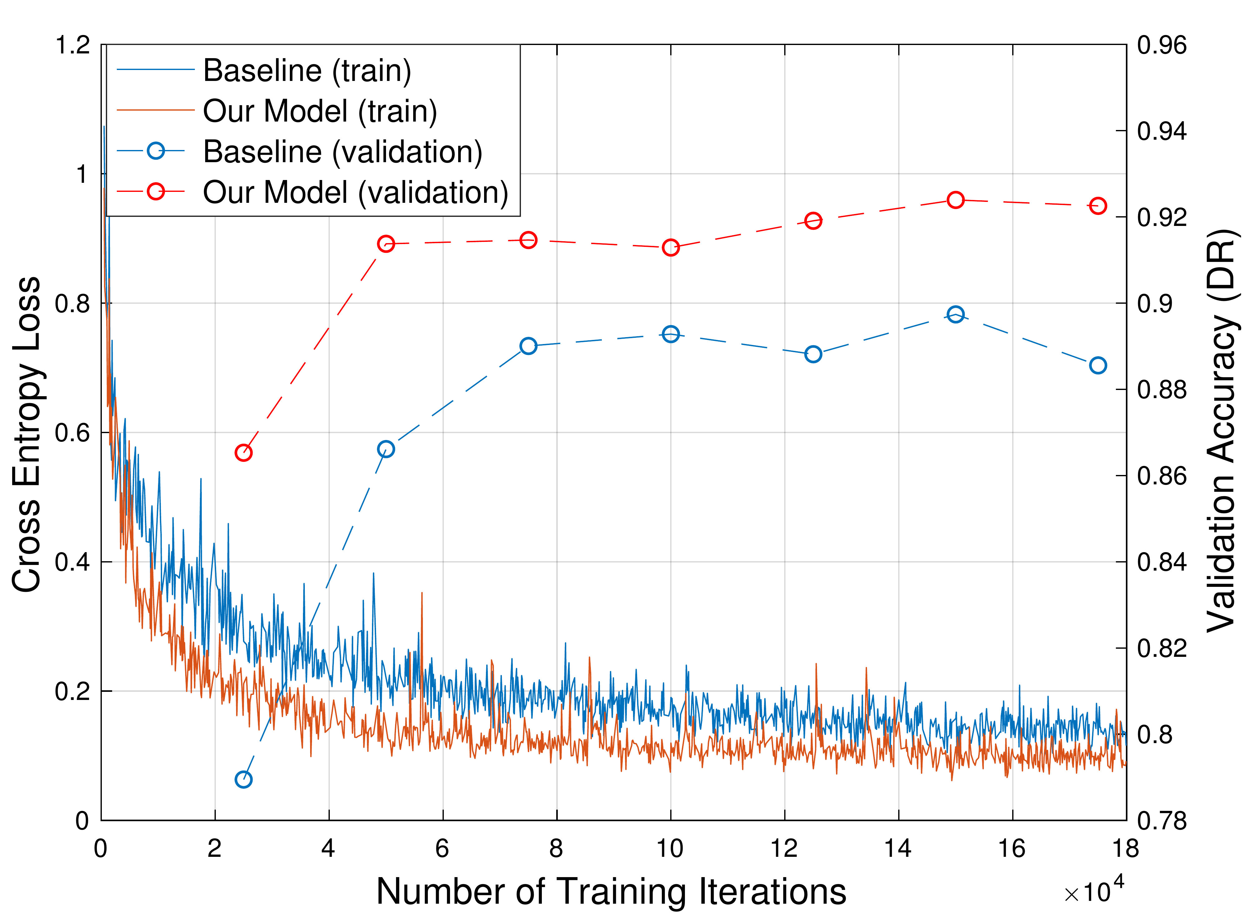
Figure 5: Comparison of training processes and validation results between our proposed model and the baseline model when training on the first 9 subjects and using the $10^{th}$ subject for validation.

Table 6: Ablation study by comparing segmentation performance between different models in terms of DR. All models are trained on the first 9 subjects and evaluated on the $10^{th}$ subject. Larger values indicate better performance. Details of models are provided in the text.

Model	CSF	GM	WM	Average
Model1	0.9585	0.9099	0.8625	0.9103
Model2	0.9568	0.9172	0.8728	0.9156
Model3	0.9576	0.9198	0.8749	0.9174
Model4	0.9578	0.9210	0.8769	0.9186
Model5	0.9554	0.9225	0.8804	0.9194
Non-local U-Net	0.9572	0.9278	0.8867	0.9239

Table 7: Ablation study by comparing segmentation performance between different models in terms of 3D-MHD. All models are trained on the first 9 subjects and evaluated on the $10^{th}$ subject. Smaller values indicate better performance. Note that 3D-MHD gives different results from MHD. Details of models are provided in the text.

Model	CSF	GM	WM	Average
Model1	0.2363	0.6277	0.4705	0.4448
Model2	0.2404	0.6052	0.4480	0.4312
Model3	0.2392	0.5993	0.4429	0.4271
Model4	0.2397	0.5926	0.4336	0.4220
Model5	0.2444	0.5901	0.4288	0.4211
Non-local U-Net	0.2477	0.5692	0.4062	0.4077

Ablation Studies of Different Modules

We perform ablation studies to show the effectiveness of each part of our non-local U-Nets. Specifically, we compare the following models:

Model1 is a 3D U-Net without short-range residual connections. Down-sampling and up-sampling are implemented by convolutions and deconvolutions with a stride of 2, respectively. The bottom block is simply a convolutional layer. Note that the baseline model, CC-3D-FCN, has showed improved performance over 3D U-Net (?). However, the original 3D U-Net was not designed for this task (?). In our experiments, we appropriately set the hyperparameters of 3D U-Net and achieve better performance.

Model2 is Model1 with short-range residual connections, i.e., the blocks in Fig. 2(a) and (b) are applied. The bottom block and up-sampling blocks are the same as those in Model1.

Model3 replaces the first up-sampling block in Model2 with the block in Fig. 2(d).

Model4 replaces both up-sampling blocks in Model2 with the block in Fig. 2(d).

Model5 replaces the bottom block in Model2 with the block in Fig. 2(c).

All models are trained on the first 9 subjects. We report the segmentation performance on the $10^{th}$ subject in Table 6 and Table 7. The results demonstrate how different global aggregation blocks in our non-local U-Nets improve the performance.

Impact of the Overlapping Step Size

As discussed above, a small overlapping step size usually results in better segmentation, due to the ensemble effect. However, with a small overlapping step size, the model has to perform inference for more validation patches and thus decreases the inference speed. We explore the trade-off in our non-local U-Nets by setting the overlapping step sizes to 4, 8, 16, 32, respectively. Again, we train our model on the first 9 subjects and perform evaluation on the $10^{th}$ subject. The patch size is set to $32^{3}$. According to the overlapping step sizes, 11880, 1920, 387, 80 patches need to be processed during inference, as shown in Fig. 7. In addition, Fig. 6 plots the changes of segmentation performance in terms of DR. Obviously, 8 and 16 are good choices that achieve accurate and fast segmentation results.

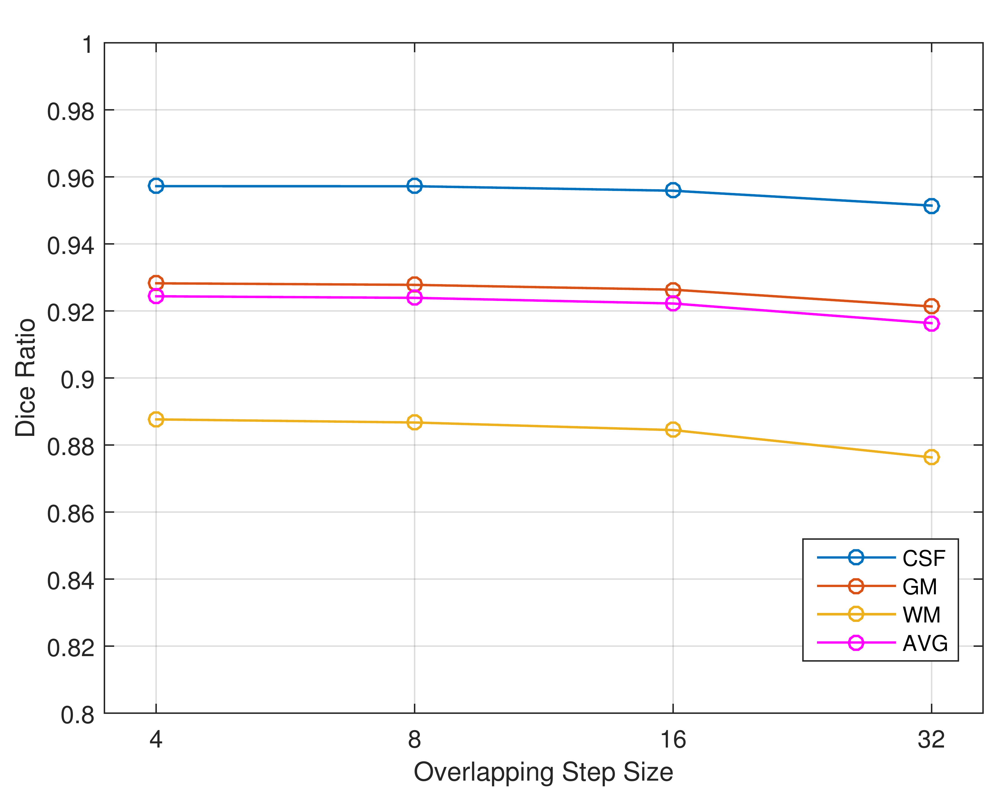
Figure 6: Changes of segmentation performance in terms of DR, with respect to different overlapping step sizes during inference. The model is trained on the first 9 subjects and evaluated on the $10^{th}$ subject.

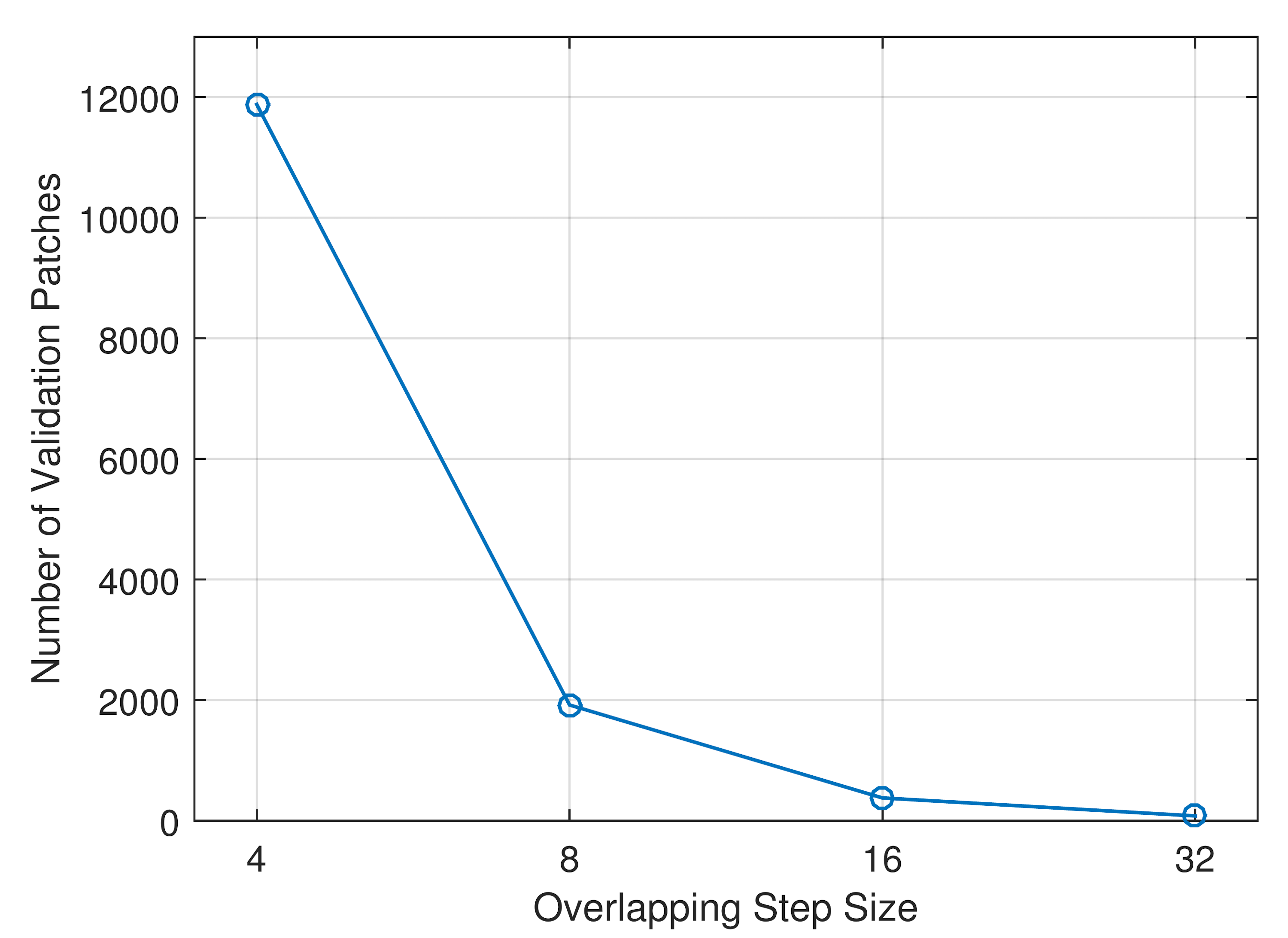
Figure 7: Changes of the number of validation patches for the $10^{th}$ subject, with respect to different overlapping step sizes during inference.

Impact of the Patch Size

The patch size affects the total number of distinct training samples. Meanwhile, it controls the range of available global information when performing segmentation for a patch. To choose the appropriate patch size for the non-local U-Nets, we perform a grid search by training on the first 9 subjects and evaluating on the $10^{th}$ subject with the overlapping step size of 8. Experiments are conducted with five different patch sizes: $16^{3}$, $24^{3}$, $32^{3}$, $40^{3}$, $48^{3}$. The results are provided in Fig. 8, where $32^{3}$ obtains the best performance and is selected as the default setting of our model.

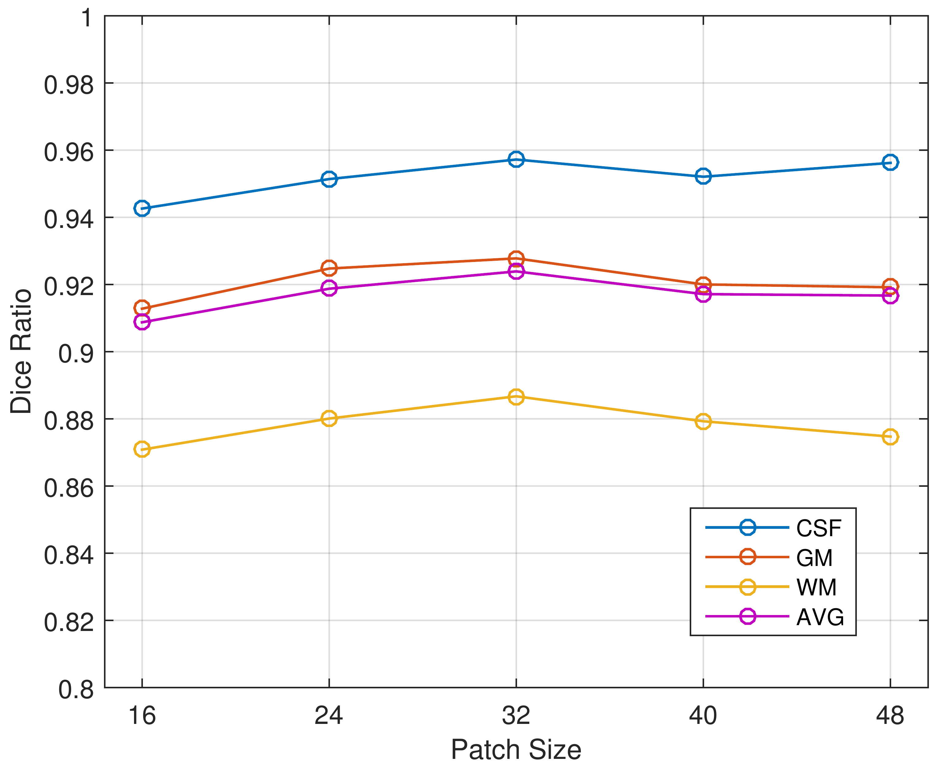
Figure 8: Changes of segmentation performance in terms of DR, with respect to different patch sizes. The model is trained on the first 9 subjects and evaluated on the $10^{th}$ subject.

Conclusion

In this work, we propose the non-local U-Nets for biomedical image segmentation. As pointed out, prior U-Net based models do not have an efficient and effective way to aggregate global information by using stacked local operators only, which limits their performance. To address these problems, we propose a global aggregation block which can be flexibly used in U-Net for size-preserving, down-sampling and up-sampling processes. Experiments on the 3D multimodality isointense infant brain MR image segmentation task show that, with global aggregation blocks, our non-local U-Nets outperform previous models significantly with fewer parameters and faster computation.

References

- [Chen et al. 2018] Chen, L.-C.; Papandreou, G.; Kokkinos, I.; Murphy, K.; and Yuille, A. L. 2018. Deeplab: Semantic image segmentation with deep convolutional nets, atrous convolution, and fully connected crfs. IEEE transactions on pattern analysis and machine intelligence 40(4):834–848.
- [Çiçek et al. 2016] Çiçek, Ö.; Abdulkadir, A.; Lienkamp, S. S.; Brox, T.; and Ronneberger, O. 2016. 3d u-net: learning dense volumetric segmentation from sparse annotation. In Proceedings of the international conference on medical image computing and computer-assisted intervention, 424–432. Springer.
- [Criminisi and Shotton 2013] Criminisi, A., and Shotton, J. 2013. Decision forests for computer vision and medical image analysis. Springer Science & Business Media.
- [Dubuisson and Jain 1994] Dubuisson, M.-P., and Jain, A. K. 1994. A modified hausdorff distance for object matching. In Proceedings of the 12th international conference on pattern recognition, volume 1, 566–568. IEEE.
- [Fakhry, Zeng, and Ji 2017] Fakhry, A.; Zeng, T.; and Ji, S. 2017. Residual deconvolutional networks for brain electron microscopy image segmentation. IEEE transactions on medical imaging 36(2):447–456.
- [Gao et al. 2019] Gao, H.; Yuan, H.; Wang, Z.; and Ji, S. 2019. Pixel transposed convolutional networks. IEEE transactions on pattern analysis and machine intelligence.
- [He et al. 2016a] He, K.; Zhang, X.; Ren, S.; and Sun, J. 2016a. Deep residual learning for image recognition. In Proceedings of the IEEE conference on computer vision and pattern recognition, 770–778.
- [He et al. 2016b] He, K.; Zhang, X.; Ren, S.; and Sun, J. 2016b. Identity mappings in deep residual networks. In Proceedings of the European conference on computer vision, 630–645. Springer.
- [Ioffe and Szegedy 2015] Ioffe, S., and Szegedy, C. 2015. Batch normalization: Accelerating deep network training by reducing internal covariate shift. In Proceedings of the international conference on machine learning, 448–456.
- [Kamnitsas et al. 2017] Kamnitsas, K.; Ledig, C.; Newcombe, V. F.; Simpson, J. P.; Kane, A. D.; Menon, D. K.; Rueckert, D.; and Glocker, B. 2017. Efficient multi-scale 3d cnn with fully connected crf for accurate brain lesion segmentation. Medical image analysis 36:61–78.
- [Kingma and Ba 2014] Kingma, D. P., and Ba, J. 2014. Adam: A method for stochastic optimization. arXiv preprint arXiv:1412.6980.
- [Krogh and Hertz 1992] Krogh, A., and Hertz, J. A. 1992. A simple weight decay can improve generalization. In Advances in neural information processing systems, 950–957.
- [Lee et al. 2017] Lee, K.; Zung, J.; Li, P.; Jain, V.; and Seung, H. S. 2017. Superhuman accuracy on the snemi3d connectomics challenge. arXiv preprint arXiv:1706.00120.
- [Lin et al. 2017a] Lin, G.; Milan, A.; Shen, C.; and Reid, I. 2017a. Refinenet: Multi-path refinement networks for high-resolution semantic segmentation. In Proceedings of the IEEE conference on computer vision and pattern recognition.
- [Lin et al. 2017b] Lin, T.-Y.; Dollár, P.; Girshick, R.; He, K.; Hariharan, B.; and Belongie, S. 2017b. Feature pyramid networks for object detection. In Proceedings of the IEEE conference on computer vision and pattern recognition, 2117–2125.
- [Long, Shelhamer, and Darrell 2015] Long, J.; Shelhamer, E.; and Darrell, T. 2015. Fully convolutional networks for semantic segmentation. In Proceedings of the IEEE conference on computer vision and pattern recognition, 3431–3440.
- [Milletari, Navab, and Ahmadi 2016] Milletari, F.; Navab, N.; and Ahmadi, S.-A. 2016. V-net: Fully convolutional neural networks for volumetric medical image segmentation. In Proceedings of the 4th international conference on 3D vision, 565–571. IEEE.
- [Nie et al. 2018] Nie, D.; Wang, L.; Adeli, E.; Lao, C.; Lin, W.; and Shen, D. 2018. 3-d fully convolutional networks for multimodal isointense infant brain image segmentation. IEEE transactions on cybernetics.
- [Ronneberger, Fischer, and Brox 2015] Ronneberger, O.; Fischer, P.; and Brox, T. 2015. U-net: Convolutional networks for biomedical image segmentation. In Proceedings of the international conference on medical image computing and computer-assisted intervention, 234–241. Springer.
- [Srivastava et al. 2014] Srivastava, N.; Hinton, G.; Krizhevsky, A.; Sutskever, I.; and Salakhutdinov, R. 2014. Dropout: A simple way to prevent neural networks from overfitting. Journal of machine learning research 15(1):1929–1958.
- [Vaswani et al. 2017] Vaswani, A.; Shazeer, N.; Parmar, N.; Uszkoreit, J.; Jones, L.; Gomez, A. N.; Kaiser, Ł.; and Polosukhin, I. 2017. Attention is all you need. In Advances in neural information processing systems, 6000–6010.
- [Wang and Ji 2018] Wang, Z., and Ji, S. 2018. Smoothed dilated convolutions for improved dense prediction. In Proceedings of the 24th ACM SIGKDD international conference on knowledge discovery and data mining, 2486–2495. ACM.
- [Wang et al. 2015] Wang, L.; Gao, Y.; Shi, F.; Li, G.; Gilmore, J. H.; Lin, W.; and Shen, D. 2015. Links: Learning-based multi-source integration framework for segmentation of infant brain images. Neuroimage 108:160–172.
- [Wang et al. 2018] Wang, X.; Girshick, R.; Gupta, A.; and He, K. 2018. Non-local neural networks. In Proceedings of the IEEE conference on computer vision and pattern recognition, 7794–7803.
- [Yuan et al. 2018] Yuan, H.; Cai, L.; Wang, Z.; Hu, X.; Zhang, S.; and Ji, S. 2018. Computational modeling of cellular structures using conditional deep generative networks. Bioinformatics 35(12):2141–2149.
- [Yuan et al. 2019] Yuan, H.; Zou, N.; Zhang, S.; Peng, H.; and Ji, S. 2019. Learning hierarchical and shared features for improving 3d neuron reconstruction. In Proceedings of the 2019 IEEE international conference on data mining. IEEE.
- [Zhang et al. 2015] Zhang, W.; Li, R.; Deng, H.; Wang, L.; Lin, W.; Ji, S.; and Shen, D. 2015. Deep convolutional neural networks for multi-modality isointense infant brain image segmentation. Neuroimage 108:214–224.
- [Zhang, Brady, and Smith 2001] Zhang, Y.; Brady, M.; and Smith, S. 2001. Segmentation of brain mr images through a hidden markov random field model and the expectation-maximization algorithm. IEEE transactions on medical imaging 20(1):45–57.