Superluminous Supernovae from the Dark Energy Survey

Abstract

We present a sample of 21 hydrogen-free superluminous supernovae (SLSNe-I), and one hydrogen-rich SLSN (SLSN-II) detected during the five-year Dark Energy Survey (DES). These SNe, located in the redshift range $0.220<z<1.998$, represent the largest homogeneously-selected sample of SLSN events at high redshift. We present the observed $g,r,i,z$ light curves for these SNe, which we interpolate using Gaussian Processes. The resulting light curves are analysed to determine the luminosity function of SLSN-I, and their evolutionary timescales. The DES SLSN-I sample significantly broadens the distribution of SLSN-I light curve properties when combined with existing samples from the literature. We fit a magnetar model to our SLSNe, and find that this model alone is unable to replicate the behaviour of many of the bolometric light curves. We search the DES SLSN-I light curves for the presence of initial peaks prior to the main light-curve peak. Using a shock breakout model, our Monte Carlo search finds that 3 of our 14 events with pre-max data display such initial peaks. However, 10 events show no evidence for such peaks, in some cases down to an absolute magnitude of $<-16$, suggesting that such features are not ubiquitous to all SLSN-I events. We also identify a red pre-peak feature within the light curve of one SLSN, which is comparable to that observed within SN2018bsz.

1 Introduction

The emergence of deeper, higher cadence transient surveys in recent years has overturned the astrophysical community’s view of the variable universe, uncovering previously unidentified classes of transient events. Superluminous supernovae (SLSNe) represent one such group of objects. These events are capable of reaching luminosities more than 10 times brighter than classical type Ia supernovae (SNe Ia), with long-lived optical light curves (e.g., Smith et al., 2007; Pastorello et al., 2010; Quimby et al., 2011; Gal-Yam, 2012, see Howell 2017 for a recent review). Originally recognised as objects peaking with an absolute magnitude of less than $-21$ (Gal-Yam, 2012), it is now apparent that SLSNe occupy a wider range of luminosities, with peak luminosities reportedly as faint as $M\sim-20$ and evolutionary timescales spanning more than a factor of five (e.g. Nicholl et al., 2015a; Inserra et al., 2017; Lunnan et al., 2018; De Cia et al., 2018).

SLSNe exhibit spectral diversity, with hydrogen-rich (SLSN-II) and hydrogen-poor (SLSN-I) varieties (and some with hydrogen only at later times, e.g., Yan et al., 2015, 2017). The luminosity and hydrogen signature of SLSNe-II can be explained by interaction between the SN ejecta and surrounding circumstellar material (CSM; Ofek et al., 2014; Inserra et al., 2018a). However, the mechanism behind SLSNe-I remains unclear: SLSNe-I can produce luminosities in excess of $\simeq$10⁴⁴ erg s^-1, and radiate total energies of $\simeq$10⁵¹ erg, exceeding the energies produced by classical core-collapse SNe by a factor of 100. Such luminosities would require several solar masses of ⁵⁶Ni to be synthesised during the explosion. Whilst the production of high ⁵⁶Ni masses is physically possible under exotic explosions paradigms such as Pair Instability SNe (Kasen et al., 2011), these models fail to replicate many observable properties of SLSN (e.g. light curve evolution), thus an additional energy input is required to boost their luminosities. Such an engine may take the form of accretion onto a central compact object (Dexter & Kasen, 2013), or the spin down of a newly-formed magnetar (Woosley, 2010; Kasen & Bildsten, 2010). The ability of this latter engine to replicate a large fraction of SLSN-I light curves is encouraging (e.g. Inserra et al., 2013; Nicholl et al., 2013; Nicholl et al., 2017b), while spectroscopic models of magnetar driven SLSNe-I ejecta are consistent with the observed spectra of SLSNe-I at early times (Dessart et al., 2012; Mazzali et al., 2016; Dessart, 2019), although the mechanism through which energy is transferred from magnetar to the ejecta is still poorly understood.

The optical pre-maximum spectra of SLSNe-I are blue and rather featureless, with characteristic broad O ii absorption lines (Quimby et al., 2011) as the defining feature, but in the ultraviolet (UV) there are several strong absorption features. The strongest lines have been identified as Fe iii, C iii, C ii, Mn ii, Si iii and Mg ii (Quimby et al., 2011; Dessart et al., 2012; Howell et al., 2013; Mazzali et al., 2016; Quimby et al., 2018), with possible variation from event to event (see detailed discussion in Quimby et al., 2018). By 30 rest-frame days after maximum light, SLSNe-I then have a tendency to resemble both normal and broad-lined type Ic SNe at peak (Pastorello et al., 2010; Liu et al., 2017). There remains discussion over the presence of various possible sub-groups within this spectral class (e.g., Gal-Yam, 2012; Inserra et al., 2018c; Quimby et al., 2018; Nicholl et al., 2019).

Significant diversity can be observed within samples of published SLSNe-I, both in light curve evolution (Lunnan et al., 2018; De Cia et al., 2018) and spectroscopic behaviour (Nicholl et al., 2015a; Inserra et al., 2017; Quimby et al., 2018). A large number of single-object studies have also been published, often highlighting ‘unusual’ features about a particular event. This makes it difficult to identify the properties of a ‘typical’ SLSN-I. For instance, the presence of a precursor bump that precedes the rise of the main light curve peak, observed in the optical light curves of some SLSNe-I (Leloudas et al., 2012; Nicholl et al., 2015a; Smith et al., 2016), has been suggested to be common to all SLSN-I events (Nicholl & Smartt, 2016), and may have been previously missed (or fallen below the detection limit) in discovery surveys. At present we can only make tentative estimates of a rate (Nicholl & Smartt, 2016) based upon limited heterogeneous samples, and as such the influence of bumps upon the physical mechanisms of SLSNe-I can only be considered on a transient-by-transient basis.

The presence of slowly-evolving SLSNe-I also complicates the issue. While samples are currently small in number, a significant fraction of these events appear to show complex fluctuations in their late-time light curves. These may be a consequence of changes in opacity as more highly ionized layers of ejecta from hard magnetar radiation reach the edge of the photosphere (Metzger et al., 2014), or could involve a less uniform ejecta structure (Inserra et al., 2017), although more detailed radiative transfer modelling is required to disentangle the two scenarios. Additional instances of slowly-evolving SLSNe-I whose declines appear to be consistent with the decay rate of ⁵⁶Ni have emerged (Lunnan et al., 2016). At present it is unclear whether such events represent a different class of transient with a different mechanism for explosion, or whether they are simply the extremes of a more continuous distribution of luminous transients.

Despite being intrinsically rare (Quimby et al., 2013; McCrum et al., 2015; Prajs et al., 2016), their extreme optical luminosities means that surveys can detect examples across large search volumes, and there are now many discoveries of SLSNe-I. Larger samples ($\sim 20$) of SLSNe-I identified within single surveys such as PanSTARRS (Lunnan et al., 2018) and the Palomar Transient Factory (PTF, De Cia et al., 2018) have provided a base for a collective analysis of homogeneously-selected SLSNe-I. However, due to the respective depths of these surveys, these samples are limited to either the local Universe (PTF, De Cia et al., 2018) or to redshifts of $z\sim 1.6$ (PanSTARRS, Lunnan et al., 2018). The Dark Energy Survey (DES), whose SN program provides high cadence, deep optical imaging for identifying transients, presents an unrivalled dataset for identifying and studying SLSNe at higher redshift. Here we present the sample of SLSNe-I identified over the five-year duration of DES. We describe our observations and outline our handling of the data in Section 2, and we overview the various analytical techniques in Section 3. We present the derived characteristics of our sample SNe in Sections 4 and 5. The host galaxies of the sample are presented within Section 6. We discuss our findings and their implications in Section 7, and finally present our conclusions in Section 8.

Throughout this paper we assume a flat $\Lambda$CDM cosmology and adopt values of $H_{0}=70.0$ km s^-1 Mpc^-1, and $\Omega_{\textrm{M}}=0.3$.

2 Observations

2.1 The Dark Energy Survey

The Dark Energy Survey (DES; The Dark Energy Survey Collaboration, 2005; Dark Energy Survey Collaboration et al., 2016) is an optical imaging survey covering 5000 deg² of the southern sky for the purpose of measuring the dark energy equation of state. Observations are carried out using the Dark Energy Camera (DECam; Flaugher et al., 2015) on the 4-m Blanco Telescope at the Cerro Tololo InterAmerican Observatory (CTIO) in Chile. The DES-SN program (DES-SN; Bernstein et al., 2012), which uses $\approx$ 10 per cent of the total survey time, surveys 10 DECam pointings, imaging 27 deg² in $g$, $r$, $i$ and $z$ filters with an approximate 7-day cadence. For a detailed discussion of the DES-SN observing strategy see Kessler et al. (2015); Diehl et al. (2018).

Although the depth of DES provides multi-colour light curves of SLSNe out to high redshift, the 5-month observing season (mid-August to early-February each year) can result in some SLSNe subject to temporal edge effects, particularly at high redshift where time dilation stretches the time-span of the transient’s visibility in the observer frame. An additional programme, the ‘Search Using DECam for Superluminous Supernovae’ (SUDSS; PI: Sullivan), was used to supplement the standard DES season with additional epochs. These observations have an approximate 14 day cadence, which extends the total coverage on selected fields to approximately eight months.

All DES survey images are processed within the DES Data Management system (DESDM; Sevilla et al., 2011; Mohr et al., 2012; Desai et al., 2012; Morganson et al., 2018). The outputs from this are then subject to difference imaging using the DiffImg pipeline (Kessler et al., 2015; Goldstein et al., 2015), a standard pipeline for transient detection in the DES-SN fields which uses deep templates from stacked epochs from previous seasons. The exception are Year 1 (Y1) transients, for which templates are drawn from observations taken within Y2. Transients are then identified using Source Extractor (SExtractor Bertin & Arnouts, 1996); see Papadopoulos et al. (2015) for further details.

2.2 The DES SLSN sample

The DES-SN programme has successfully identified several SLSN candidates (e.g., see Papadopoulos et al., 2015; Smith et al., 2016; Pan et al., 2017; Smith et al., 2018). SLSNe are not explicitly selected for follow up by their luminosity, but were identified and prioritized for spectroscopic follow up based upon combinations of the following criteria:

1. Where the SN rise is visible within the data, the light curve must display a slow ($>25$ day) rise time in the observer frame.

2. Where only the SN decline is visible within the data, the light curve must be visible for $>25$ days and must exhibit a slow ($<0.1$ mag day^-1) rate.

3. The transient is predominantly blue in colour ($g-r$ <1.0 or $r-i$ <1.0 mag).

4. The transient must exhibit colour evolution during the decline (to avoid AGN contamination).

5. The transient resides within a faint ($\Delta m_{\mathrm{host-sn}}>0.7$) or undetected host galaxy within the template DES images .

These criteria are soft cuts designed designed such that they should encapsulate the photometric properties of the vast majority of literature SLSNe as observed within any given DES season, whilst excluding obvious contaminants such as SNe-Ia and AGN flares. They also employed for the selection of the photometric SLSN sample from DES (Thomas et al. in prep.). Potential biases in the selection of this sample are discussed within Section 7.3.

2.2.1 Spectra

We triggered spectroscopic observations for a total of 30 SN candidates whose properties met the above criteria across a variety of telescopes under the follow-up programmes designed to catch any SN whose properties did not fall into classical paradigms (i.e. not typical SNe Ia, SNe Ibc or SNe II). In addition, two other SNe were initially identified as potential SN Ia candidates by the Photometric SN IDentification software (psnid; Sako et al., 2011) used to prioritize spectroscopic follow-up (D’Andrea et al. in prep.) and were observed under various SN-Ia programmes prior to classification as SLSNe (see also Pan et al., 2017).

Object classifications were performed using superfit (Howell et al., 2005), implementing the comprehensive spectral template library of Quimby et al. (2018). We assign the classification of SLSN-I based upon their spectral similarity to other known SLSNe-I within the literature: well described by a hot black body continuum at early times, with broad absorption lines produced by C, O, Si, Mg, and Fe with high velocities ($\sim 10000$ km s⁻¹). High redshift events can also be identified by the presence of absorption below rest-frame 3000Å due to heavy elements (Fe, Co, Ti) and highly ionised CNO-group elements (Mazzali et al., 2016). Unlike SNe Ia, the observed spectral features of a SLSN cannot necessarily be used to determine its exact phase. The spectral features observed are a function of the photospheric temperature of the SLSNe, and as SLSNe have been shown to evolve on a variety of different timescales (Nicholl et al., 2017b), this results in a much broader range of epochs over which a given spectral feature may be observed. As such, we do not require the epoch of the classification spectrum and that of the best matching spectral template to exactly coincide, allowing them to agree within $\sim\pm 10$ days.

We assign the spectroscopic classification of SLSN-I for objects based upon spectroscopic behaviour similar to other literature SLSNe-I near peak, and where we can confidently rule out the presence of hydrogen (H$\beta$ or H$\alpha$ depending upon the redshift) at the time of observation. We do not place any luminosity restrictions in our spectroscopic classification. For one of the SNe, DES17E1fgl we identify the presence of H$\beta$ at an observed wavelength of 7388Å, although the spectrum does not extend to redder wavelengths to confirm this classification with the addition of H$\alpha$ emission, so we thus classify this object to be ‘hydrogen-rich SLSN-like’ (‘SLSNe-II’).

Where the signal-to-noise ratio of the classification spectra is low ($\lesssim 10$), or the match to spectral templates is visually poor, or the spectrum does not have adequate wavelength coverage to highlight these features which occur prominently in the rest-frame UV, we also consider the rankings of the best fitting spectral templates, as determined by superfit. We use the average rank of the templates of each spectroscopic class, whereby spectroscopic classes whose templates typically rank higher are used as a provisional classification. In such scenarios, we qualify the classification as ‘Silver’ (as opposed to ‘Gold’ where the match is more certain). This happened in only two cases.

Where possible, we estimate spectroscopic redshifts using either host galaxy emission lines (H$\beta$, [O ii] $\lambda$3727 Å, [O iii] $\lambda\lambda$ 4959, 5007 Å) or narrow host absorption features such as Mg ii $\lambda\lambda$ 2796, 2803 Å and/or Fe ii $\lambda$2344Å identified within the reduced spectra. In cases where the underlying host galaxy features could not be detected (6/22 events), we estimate the redshift from the best fitting spectral templates within superfit.

Table 1: SLSNe spectroscopically identified over the duration of the Dark Energy Survey. Redshifts are estimated from the host galaxy spectrum are marked ‘H’ and those found using the features in SN spectrum are marked ‘S’. The precision of the measured redshifts varies depending upon the method through which they were derived (redshifts found from host spectra are typically better constrained). We also assign a classification ‘standard’ of either Gold or Silver, depending upon our confidence in their classification.

DES ID	$\alpha$	$\delta$	$z$	$z$	Class	Standard	Rest-frame $\lambda$
				Source			Coverage Å
DES13S2cmm	02:42:32.83	-01:21:30.1	0.663	H	SLSN-I	Gold	2787 $\rightarrow$ 5541
DES14C1fi	03:33:49.80	-27:03:31.6	1.302	H	SLSN-I	Silver	1931 $\rightarrow$ 3840
DES14C1rhg	03:38:07.27	-27:42:45.7	0.481	S	SLSN-I	Gold	3130 $\rightarrow$ 6222
DES14E2slp	00:33:04.08	-44:11:42.8	0.57	S	SLSN-I	Silver	2952 $\rightarrow$ 5870
DES14S2qri	02:43:32.14	-01:07:34.2	1.50	S	SLSN-I	Gold	1854 $\rightarrow$ 3686
DES14X2byo	02:23:46.93	-06:08:12.3	0.868	H	SLSN-I	Gold	2492 $\rightarrow$ 4955
DES14X3taz	02:28:04.46	-04:05:12.7	0.608	H	SLSN-I	Gold	2883 $\rightarrow$ 5731
DES15C3hav	03:31:52.17	-28:15:09.5	0.392	H	SLSN-I	Gold	3335 $\rightarrow$ 6630
DES15E2mlf	00:41:33.40	-43:27:17.2	1.861	H	SLSN-I	Gold	1621 $\rightarrow$ 3222
DES15S1nog	02:52:14.98	-00:44:36.3	0.565	H	SLSN-I	Silver	2962 $\rightarrow$ 5889
DES15S2nr	02:40:44.62	-00:53:26.4	0.220	H	SLSN-I	Gold	3799 $\rightarrow$ 7554
DES15X1noe	02:14:41.93	-04:52:54.5	1.188	H	SLSN-I	Gold	2118 $\rightarrow$ 4212
DES15X3hm	02:26:54.96	-05:03:38.0	0.860	H	SLSN-I	Gold	2492 $\rightarrow$ 4955
DES16C2aix	03:40:41.17	-29:22:48.4	1.068	H	SLSN-I	Gold	2249 $\rightarrow$ 4472
DES16C2nm	03:40:14.83	-29:05:53.5	1.998	H	SLSN-I	Gold	1546 $\rightarrow$ 3074
DES16C3cv	03:27:16.71	-28:42:45.9	0.727	H	SLSN-I	Silver	2684 $\rightarrow$ 5336
DES16C3dmp	03:31:28.35	-28:32:28.3	0.562	H	SLSN-I	Gold	2961 $\rightarrow$ 5888
DES16C3ggu	03:31:12.00	-28:34:38.7	0.949	H	SLSN-I	Gold	2377 $\rightarrow$ 4726
DES17E1fgl	00:32:09.62	-42:38:49.3	0.52	H	SLSN-II	Gold	2967 $\rightarrow$ 5899
DES17X1amf	02:17:46.70	-05:36:01.0	0.92	S	SLSN-I	Gold	2414 $\rightarrow$ 4799
DES17C3gyp	03:27:51.87	-28:23:44.3	0.47	S	SLSN-I	Silver	3152 $\rightarrow$ 6268
DES17X1blv	02:20:59.64	-04:29:00.8	0.69	S	SLSN-I	Gold	2742 $\rightarrow$ 5452

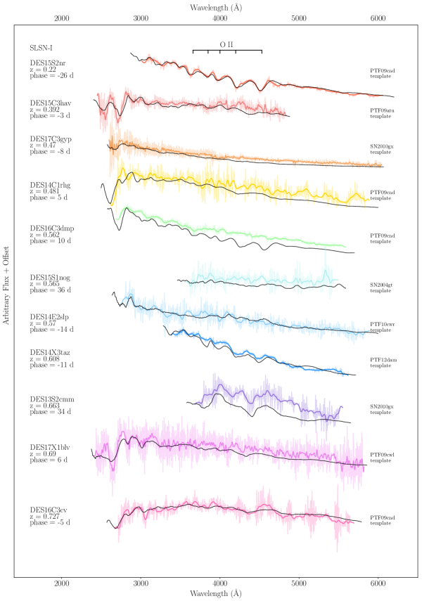
Figure 1: Spectra used for the spectroscopic confirmation of DES SLSN-I candidates, with observational details given in Table LABEL:tab:spec_obs. The DES spectra are shown unbinned and binned by 5 Å bins to increase the clarity of the features. The phase provided corresponds to the phase at which the classification spectrum was taken in the SN rest frame, not that of the spectral template. The black lines show the smoothed best fitting spectral template used to classify the spectrum for each SN (see Quimby et al. 2018 for more template details). We determine spectroscopic redshifts from either the presence of host galaxy absorption lines, or from fitting the observed SN features to those of established SLSNe within the literature. Table 1 contains details of the reshift source and classification quality for each event. Here we highlight the O ii absorption lines seen in the optical spectra around 4000Å.

Figure 1 Cont: Figure 1 continued. We highlight some of the typical spectroscopic features observed within SLSN-I at higher redshift – namely blended absorption from C, Mg, Ti and Si lines below 3000Å. We also show the spectra used to confirm our SLSN-II candidate (lower panel), with the H$\beta$ line used to classify this event highlighted in the lower right panel. Table 1 contains details of the reshift source and classification quality for each event.

From these data, we have spectroscopically identified a sample of 22 SLSNe. We present our classification spectra in Fig. 1, alongside the best fitting spectral template for each object, and details of all spectroscopic observations can be found in in Table LABEL:tab:spec_obs. Basic information on each event (including the classification quality) can be found in Table 1. Our final sample spans a broad redshift range of $0.220\leq~{}z~{}\leq 1.998$ (Fig. 2). The deep imaging capability of DES enables the detection of both local ‘fainter’ SLSNe, as well as their higher redshift counterparts, including some of the most distant spectroscopically confirmed SNe to date (Pan et al., 2017; Smith et al., 2018). This broad redshift range consequently results in a wide range of rest-frame wavelengths being probed from object to object. We list the rest-frame wavelengths of the DECam filters for each object in Table 1.

Figure 2: The redshift distribution of the DES SLSNe, grouped into bins of $z=0.2$. The median redshift of the sample is $z=0.86$.

2.2.2 Light Curves

Photometric measurements of all DES SLSNe were made using the pipeline discussed by Smith et al. (2016), which has also been extensively used in the literature (e.g., Firth et al., 2015, and references therein). This pipeline performs classical difference imaging by subtracting a deep template image (typically 4-6 times deeper than a single photometric epoch alone) from each individual SN image to remove the host-galaxy light using a point-spread-function (PSF) matching routine. SN photometry is then measured on the difference images using a PSF fitting technique. The $g,r,i$ and $z$ light curves for every confirmed DES SLSNe are presented within Fig. 3, and the photometry is given in Appendix B. All reported magnitudes are corrected for Milky Way extinction following Schlafly & Finkbeiner (2011).

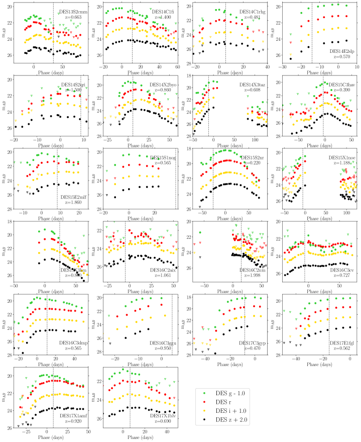
Figure 3: The DES $g,r,i,z$ light curves of our sample of SLSNe. All magnitudes are in the AB system and are corrected for Milky Way extinction. All light curves show the phase of the SNe with respect to the peak in the observer-frame $g$-band (or $r$-band for objects with no $g$-band flux). Unfilled triangles are non-detections reported as 3-$\sigma$ upper limits. For clarity the $g,i$ and $z$ bands are offset by $-1$, 1 and 2 magnitudes respectively. Dashed grey lines indicate the phases at which classification spectra were obtained.

3 Light curve interpolation

Our next task is to develop the framework to calculate SN brightnesses at any epoch by interpolating the DES observations. This is required to estimate the peak brightnesses of the SNe, as well as to estimate bolometric luminosities. In this paper we use Gaussian Process techniques to perform the light curve interpolation.

Gaussian Processes (GP) are a generalised class of functions, which may be used to model the correlated noise within time-series data. They represent a distribution over the infinite number of possible outputs of a function, such that the distribution over any finite number of them is a multivariate Gaussian. GP functions consist of a mean function ($\mu(x)$) and a ‘kernel’ ($k(x,x^{\prime})$), which is a simple function used to describe the covariance between data points $x$ and $x^{\prime}$.

$$f(x)=GP\big{(}\mu(x),k(x,x^{\prime})\big{)}$$ (1)

GPs may be considered a generalisation of a Gaussian distribution; at each point $x$, the reconstructed function $f(x)$ may be described by a normal distribution. Neighbouring points are not independent, but are related by some predetermined covariance function, given by the kernel. The use of GP techniques allows the user to marginalise over systematic sources of noise within a data, which might otherwise not be captured in an astrophysical model.

At each point in the reconstructed function, the precise value of the resultant value of the function is unknown, but does lie within a normal distribution (Rasmussen & Williams, 2006). The mean function $\mu(x)$ describes the mean value drawn from this distribution of possible answers, while the covariance function used within the GP determines the form of the relationship between surrounding data points. The covariance function used here depends upon two hyper-parameters; the variance of the signal within the function, and the characteristic scale length over which any significant signal variations occur. For time-series data, these two hyper-parameters respectively become the uncertainties in measured flux and the timescale over which significant changes occur within the data. The functional form of the covariance function or ‘kernel’ used may be selected/constructed such that it reflects any periodic tendencies within the data.

The final likelihood function of a GP is a multivariate Gaussian with $N$ dimensions, but in which the measurements are dependent as dictated by a covariance matrix, which absorbs any systematics that are unknown to the user. In order to produce the best interpolation between data points, the hyper-parameters of the kernel may be optimally fit for.

Here we interpolate the multi-colour light curves of the DES SLSNe using GP fitting. To do this we utilise the python package george (Ambikasaran et al., 2014) and optimally fit the hyper-parameters of a Matern 3/2 kernel independently for each of the $g,r,i,z$ light curves. A Matern 3/2 kernel is mathematically similar to the more familiar squared exponential function (but with a narrower peak) and has the form

$$k(r)=\sigma^{2}\bigg{(}1+\frac{{\sqrt{3}r}}{l}\bigg{)}\exp{\Bigg{(}\frac{-{\sqrt{3}r}}{l}\Bigg{)},}$$ (2)

where $\sigma$ is the uncertainty of an observation, $r$ is the separation between observations and $l$ is the characteristic scale length over which variations in the data occur.

We chose this kernel form as we find the sharper peak results in greater flexibility within the final function over short timescales, which acts to best capture the visual form of the SLSN light curves. Prior to interpolation, we perform a gradient based optimization to determine the best fitting hyper-parameters for the kernel in each photometric band. We interpolate the observations using GPs over regions where we have SN detections in multiple bands. For SN detected over multiple seasons, the interpolation is carried out over the entire duration of the transient, although we note that between observing epochs the interpolation is highly unconstrained.

The independent fitting of the $g,r,i,z$ light curves fails to take into account any wavelength overlap between the DECam photometric filters. Given the fairly even sampling of the survey across all 4 filters, it is possible to improve constraints upon the light curve behaviour through the use of a 2-dimensional kernel in which the wavelength scale is also accounted for. However, a 2-dimensional kernel is beyond the aims of this study.

For each GP fit, we present the mean and 1$\sigma$ uncertainties in Fig. 4, with the DES photometry. With each optimised kernel, the interpolated light curves have less flexibility in areas with a greater data density (where the data points are well constrained), as the underlying trend can be specified at a higher confidence. Conversely, interpolations during large gaps in the data are more uncertain.

Visual inspection of the final interpolations in Fig. 4 shows that they capture the evolution of the SLSN well. We do observe some ‘ballooning’ of the uncertainties between well constrained data points where the gap between observations is large (for example, the light curve of DES16C3dmp shows such a feature between observations at $+18$ and $+28$ days). This is a natural consequence of the GP interpolation, as the optimised kernel determines the coherence between observations. High cadence, well-constrained observations result in fewer degrees of freedom for the fit between observations. More sparsely spaced, but well constrained observations in the light curve will generate more uncertainty in the final fit.

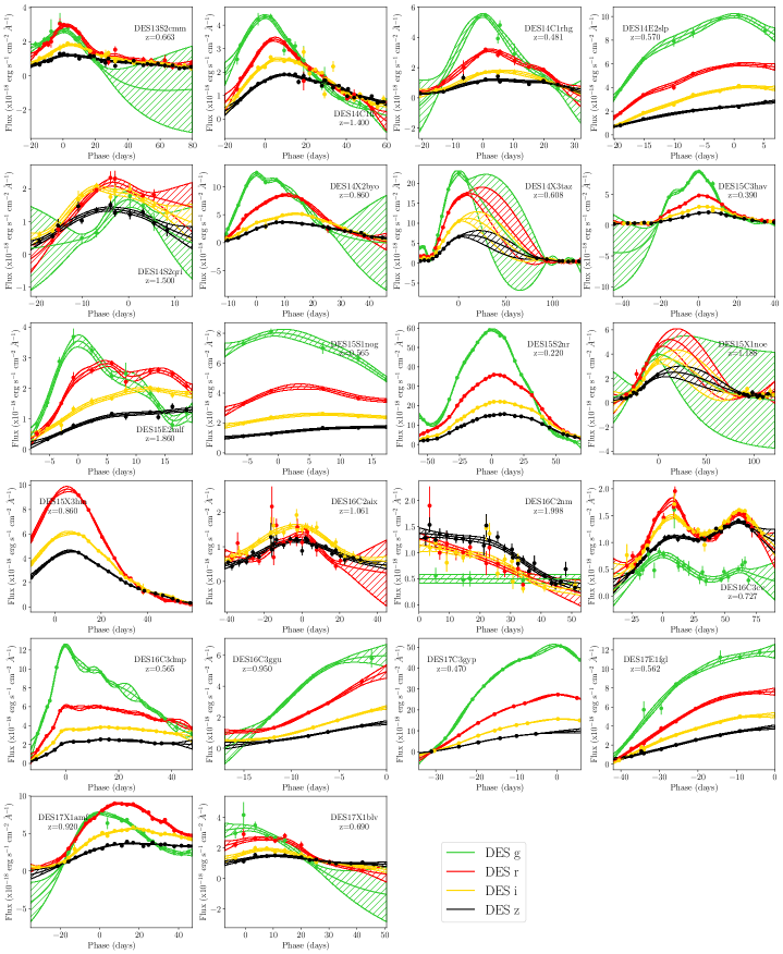
Figure 4: The $g,r,i$ and $z$ Gaussian Process interpolated light curves of DES SLSNe using an optimised Matern 3/2 kernel. Limits are not shown here. All light curves show the phase of the SNe with respect to the peak in the observer-frame $g$-band (or $r$-band for objects with no $g$-band flux). These interpolated light curves are used in Sections 3, and 4 to determine the light curve parameters and to fit physical models to the data.

The interpolated fits provided by the GP provide photometry estimates at any epoch, regardless of the spacing in the observations. This allows an estimation of the peak epoch of the SN, as well as its evolutionary timescales. We define these light curve properties for each in SN in its bluest observed band (either DES $g$ or $r$, depending on the redshift), using the GP interpolated fits to determine the peak MJD, rise and decline times. These properties are presented in Table LABEL:tab:slsnphot.

4 Modelling the Light curves

In order to investigate the emerging diversity of physical characteristics attributed to SLSNe within the literature, it is necessary to apply models to the observed light curves such that their the rest frame properties can be determined. We fit the following physical models to the interpolated DES SLSN light curves; a modified black body and a magnetar model.

4.1 A modified black body model

For simplicity in determining luminosities and k-corrections for our light curves, we use an approximate spectral energy distribution (SED) to generate synthetic photometry and fit this to the data. While SLSNe-I present largely featureless spectra in relation to other SN classes, fairly well represented by a black body at optical to NIR wavelengths (e.g. Nicholl et al., 2017b), they deviate from a black body SED at ultraviolet (UV) wavelengths, with significant absorption below $\sim$<3000 Å. These features, largely attributed to absorption by heavy elements (see Mazzali et al., 2016, for example line identification), will dominate the observable optical light curves of the higher redshift SLSNe found within DES. We therefore adopt a modified black body model for our SLSN SEDs.

We construct our modified SEDs in the following manner. We use empirical templates of UV absorption based upon 110 rest-frame spectra of SLSNe-I (as per Inserra et al., 2018d), from which we estimate the variation of UV absorption at temperatures of 15000 K, 12000 K, 10000 K, 8000 K and 6000 K (corresponding to the following approximate phases respectively; $<10$ days, $10<$phase$<15$ days, $15<$phase$<22$ days, $22<$phase$<35$ days and $>35$ days from peak) . These spectroscopic templates are presented within Fig. 5. Due to a lack of spectroscopic information bluewards of $\sim 2000-2500$ Å depending upon the temperature/phase of the SN, we model our SEDs shortwards of these wavelengths as that of a black body. This assumption may lead to an overestimation of flux in bolometric calculations (if a blueward bolometric correction were included), particularly around maxiumum light (i.e. the 15,000K template), when the SED peaks around this region. However, it should not impact our k-correction for blue photometric bands with wavelengths greater than $\sim$3000Å, and as only 2 objects within our sample are probed by the DES photometry at wavelengths bluer than the template boundaries (DES16C2nm and DES15E2mlf), this should not significantly impact the results presented here.

We then follow the methodology of Prajs et al. (2016), fitting the featureless regions of the continuum within the templates in 50 Å wide bins with Planck’s law. From this we determine the ratio between the template and the black body continuum that we use as measure of the strength of the absorption features as a function of wavelength. The strength of the UV absorption is highest around the peak of the SN (i.e., when the photosphere is hottest), and generally decreases in strength as the SN cools. At longer wavelengths, we assume no additional absorption and therefore adopt a standard Planck black body for the SED.

Finally, for any k-corrections to other photometric filters we use the ‘mangling’  technique of Hsiao et al. (2007) to colour correct our synthetic SEDs. We do this by fitting a spline function to our photometry and then applying this function to the SED, thus ensuring that the SED replicates the colours of our $g,r,i,z$ photometry.

Figure 5: The spectroscopic templates of SLSNe at temperatures of (bottom panel)  6000, 8000, 10000, and (top panel)  12000 and 15000 K, (corresponding phase$>35$ days, $22<$phase$<35$ days, $15<$phase$<22$ days, $10<$phase$<15$ days and $<10$ days respectively) derived from the averaged spectra of literature SLSNe with rest-frame UV coverage (as per Inserra et al., 2018b). Grey dashed lines indicate the SED of an unabsorpbed black body at the same temperature. We fit the featureless continuum regions of these spectra in 50Å wide bins with Planck’s law, and thus determine the ratio between the template and the black body SED. These final templates are applied to the DES SLSN black body SEDs to approximate the strength of UV absorption as a function of wavelength and temperature.

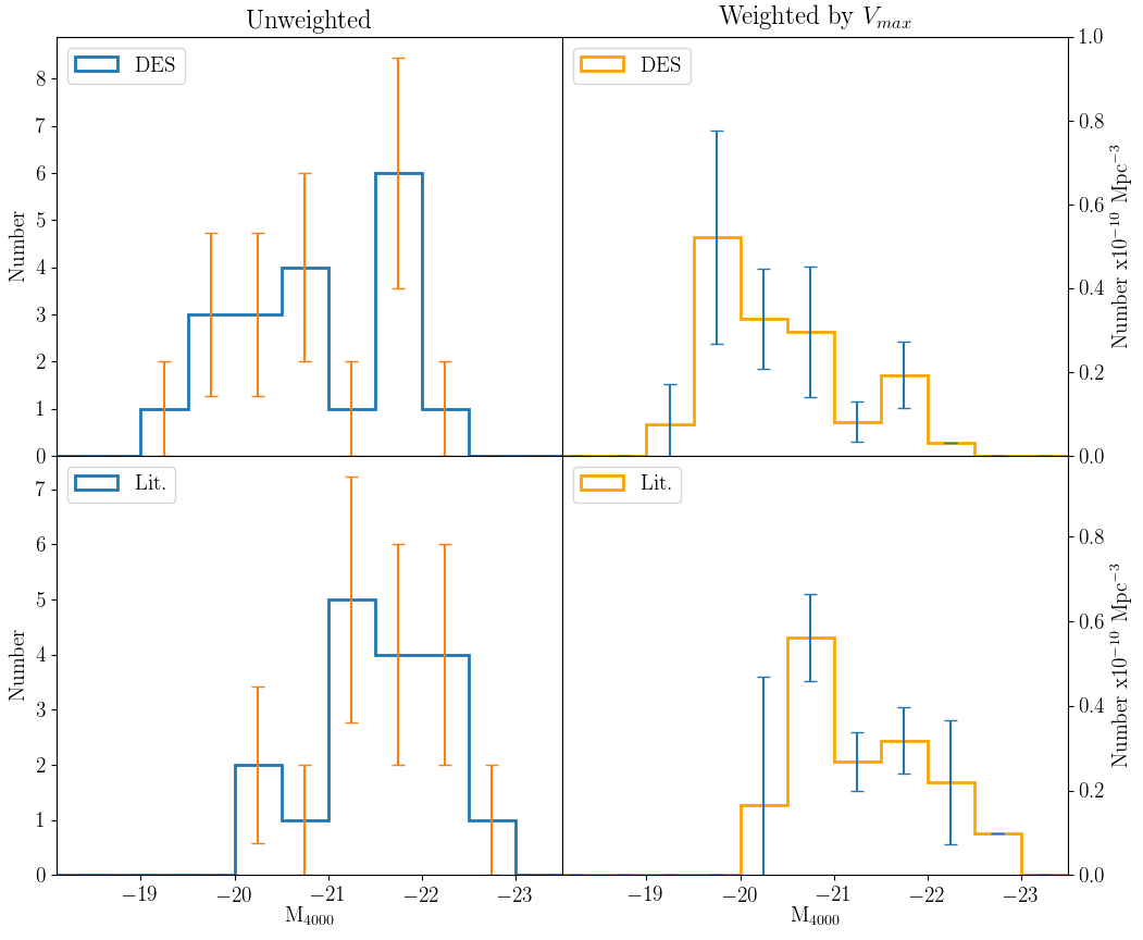
Figure 6: SLSN-I luminosity functions in the synthetic 4000 Å band (Inserra & Smartt, 2014). The panels on the left show the unweighted distributions of peak luminosities for DES SLSNe-I (top panels), and for spectroscopically-confirmed SLSNe-I from the literature (lower panels). The panels on the right show the same distributions but weighted by $1/V_{\mathrm{max}}$, the maximum volume out to which each event could have been classified. Here the sensitivity of DES highlights the presence of an increased population of events peaking at fainter luminosities.

4.1.1 The SLSN-I luminosity function

We fit our modified black body model to the GP interpolated $g,r,i,z$ light curves, with the peak temperatures and radii from these fits within Table LABEL:tab:slsnproperties. We then use these SEDs to determine the absolute peak luminosities of the SLSN light curves within the artificial 4000 Å band first defined in Inserra & Smartt (2014). This band was selected for the purposes of standardization as it encompasses a region of a typical SLSN spectrum which is usually dominated by featureless continuum for up to $\sim 30$ days after peak. We thus determine these magnitudes using the best fitting modified black body spectrum to the observed photometry of at the SN peak within the SN rest-frame. These peak luminosities are presented within Table LABEL:tab:slsnphot, and the distribution of peak magnitudes in Fig. 6.

Table 2: The derived photometric properties of the DES SLSN sample. Rise times ($\tau_{\mathrm{rise}}$) are measured using the GP interpolations, from the epoch of the last non-detection to peak brightness, and vice-versa for decline times ($\tau_{\mathrm{decline}}$).

DES ID	MJDpeak	Peak LBol	$\tau_{\mathrm{rise}}$	$\tau_{\mathrm{fall}}$	Peak M4000	Peak M5200
	(J2000)	erg s-1	(days)	(days)
DES13S2cmm	56562.4	2.043e+43	20.0	64.1	-19.63 $\pm$ 0.46	-19.96 $\pm$ 0.42
DES14C1fi	56920.8	1.481e+44	22.0	59.9	-21.96 $\pm$ 0.30	-22.36 $\pm$ 0.27
DES14C1rhg	57010.9	9.015e+42	20.9	30.0	-19.58 $\pm$ 1.01	-19.71 $\pm$ 0.68
DES14E2slp	57040.6	3.067e+43	19.9	8.02	-20.51 $\pm$ 0.07	-20.48 $\pm$ 0.06
DES14S2qri	57050.4	9.196e+43	7.6	22.4	-21.57 $\pm$ 0.19	-21.59 $\pm$ 0.18
DES14X2byo	56944.7	8.991e+43	10.0	32.2	-21.67 $\pm$ 0.13	-21.64 $\pm$ 0.12
DES14X3taz	57077.5	1.069e+44	29.1	10.9	-21.72 $\pm$ 0.20	-21.80 $\pm$ 0.18
DES15C3hav	57339.1	1.057e+43	19.9	40.0	-19.57 $\pm$ 0.60	-19.69 $\pm$ 0.47
DES15E2mlf	57348.8	2.137e+44	8.0	19.9	-21.99 $\pm$ 0.43	-21.79 $\pm$ 0.40
DES15S2nr	57318.9	1.760e+43	48.9	68.2	-20.28 $\pm$ 0.16	-20.36 $\pm$ 0.14
DES15X1noe	57423.7	1.106e+44	48.8	125.0	-23.37 $\pm$ 3.17	-24.16 $\pm$ 2.74
DES15X3hm	57229.4	1.410e+44	-	66.9	-22.00 $\pm$ 0.15	-21.86 $\pm$ 0.14
DES16C2aix	57715.1	1.257e+43	26.0	43.1	-20.81 $\pm$ 0.60	-20.99 $\pm$ 0.54
DES16C2nm	57620.0	1.062e+44	-	52.0	-22.82 $\pm$ 0.67	-23.18 $\pm$ 0.61
DES15S1nog	57365.2	1.947e+43	11.7	16.3	-20.32 $\pm$ 0.50	-20.27 $\pm$ 0.46
DES16C3cv	57665.5	1.348e+43	42.0	64.9	-19.18 $\pm$ 0.40	-19.86 $\pm$ 0.35
DES16C3dmp	57725.2	2.769e+43	10.9	42.0	-20.66 $\pm$ 0.34	-20.54 $\pm$ 0.32
DES16C3ggu	57794.2	6.531e+43	15.0	-	-21.09 $\pm$ 0.37	-20.92 $\pm$ 0.56
DES17E1fgl	58136.1	3.195e+43	42.0	-	-20.58 $\pm$ 0.18	-20.66 $\pm$ 0.16
DES17X1amf	58049.6	1.037e+44	24.2	41.9	-21.61 $\pm$ 0.42	-21.79 $\pm$ 0.38
DES17C3gyp	58049.6	7.787e+43	24.2	41.9	-21.69 $\pm$ 0.14	-21.63 $\pm$ 0.13
DES17X1blv	58049.6	1.724e+43	24.2	41.9	-20.04 $\pm$ 0.02	-20.16 $\pm$ 0.02

For comparison we also determine the 4000 Å luminosity function of other spectroscopically classified SLSNe-I from the literature. To do this we take the previously published photometry and perform GP interpolation in the same way as for the DES objects. We select the literature sample based upon the following criteria:

• Each SN must have been spectroscopically classified as a SLSN-I or ‘SLSN-I like’,

• Each SN must have been observed in a minimum of three different photometric bands for better parameterization when fitting the SEDs,

• Each observed band must have a minimum of five epochs of data.

We process the interpolated literature light curves in an analogous manner to the DES SLSNe, using the modified black body function described previously. We perform a volumetric correction to both our samples of SLSNe-I using the maximum volume over which the SNe could have been detected ($V_{\mathrm{max}}$). We use a limiting magnitude for spectroscopic confirmation of $m_{R}\sim 23.5$ mag to determine the maximum volume out to which the particular SLSN could have been spectroscopically identified. In Fig. 6, we observe a clear difference in the distributions of transient luminosities between the two samples, with the depth of DES more frequently identifying fainter SLSNe, with four SLSNe events peaking at $M>-20$, while the observational bias for spectroscopic follow up of brighter objects within literature SLSN samples skews this distribution to higher luminosities. This trend persists in the volume-corrected distributions, where we see the majority of DES objects lie fainter than the arbitrary $M<-21$ limit originally used to classify SLSNe.

This broad distribution in peak luminosities exhibited within the DES SLSN-I sample brings the congruence amongst other SLSNe into question. We therefore compare their luminosity and colour evolution using the ‘4OPS’ parameter space defined in Inserra et al. (2018c), which compares the colour and evolution in the artificial 4000 Å and 5200 Å bands which have shown to be significantly correlated for other SLSNe in the literature. We determine the 5200 Å light curves of the DES SLSNe in the same manner as their 4000 Å light curves, and using the luminosities in these bands at both peak and $+30$ day phases (where possible), place them in the 4OPS parameter space in Fig. 7.

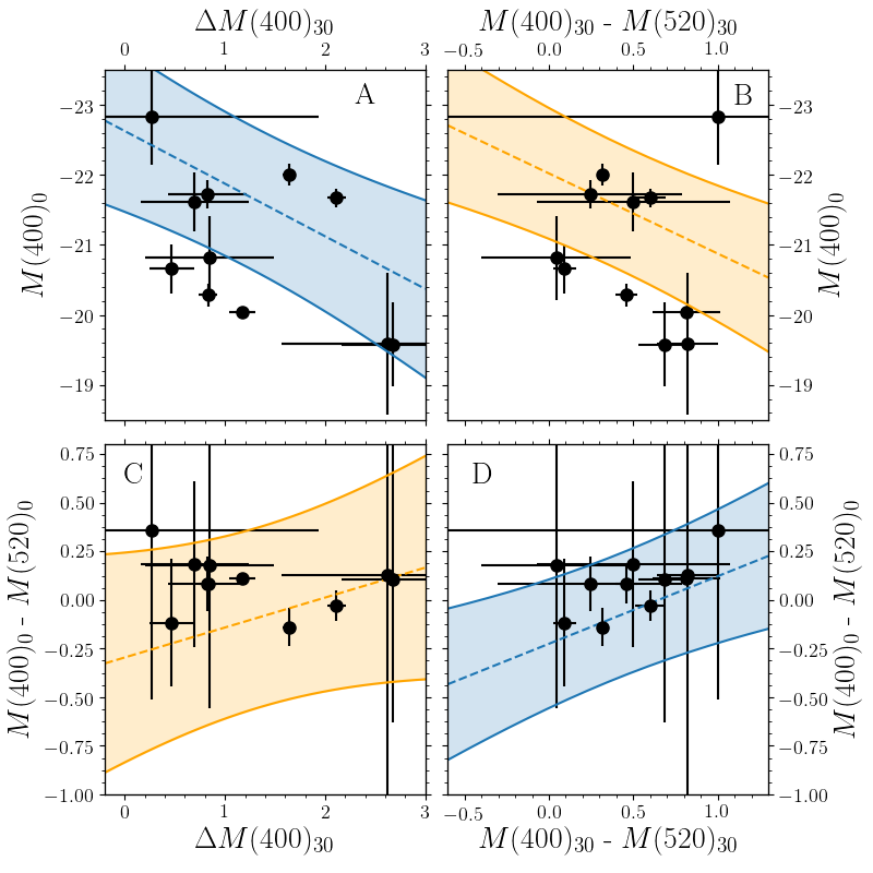
Figure 7: The ‘4OPS’ SLSN parameter space introduced by Inserra et al. (2018c), showing the statistical relations in the luminosity and colour evolution of SLSNe. Panel A (top left) shows the relationship between peak luminosity and luminosity at $+30$ days in the 4000 Å band; Panel B (top right) the relationship between the $4000-5200$ Å colour and peak 4000 Å luminosity; Panel C (bottom left) the relationship between the luminosity at 30 days and the colour at peak and finally; Panel D (bottom right), the relationship between colour at peak and colour at 30 days. The orange and blue shaded regions highlight the 3$\sigma$ confidence bands within which this parameter space has been defined for previous samples of SLSNe. Only 11 of the 22 DES SLSNe possess information at $+30$ days from maximum light, such that they can be included in the 4OPS plot. Due to the lack of data and extensive extrapolation around peak for DES15X1noe, we do not include this object within the 4OPS plot.

The 4OPS parameter space gives some insight into the physical properties of the SN ejecta, for instance a correlation between colour at two different phases suggests a link in temperature or radius of the ejecta during these epochs (Inserra et al., 2018c). Within the paradigm of the magnetar model of SLSN production, these relations have been interpreted as the energy from the magnetar being injected at the same epoch for all SLSNe (Inserra et al., 2018c), as this would naturally create a similar timescale for the rise of the SN and the diffusion timescale through the ejecta.

Whilst the DES SLSNe fall within the colour-evolutionary space defined by other SLSNe, they push the boundaries of some of these statistical relationships, with a significant fraction of the sample falling on average $\sim 1$ magnitude fainter at peak than the 3$\sigma$ space statistically occupied by other SLSN events of the same decline rate. Many events also evolve on more rapid timescales than the 3$\sigma$ parameter space originally defined with literature events too. This is likely a reflection of the softer selection criteria designed in selection of the DES SLSN sample. We do not find any significant correlation between the peak luminosities and peak colours of these events, which does not suggest a strong link between the peak luminosity and photospheric temperature for all events within the sample.

This broad spread of luminosities could be due to a range of injection times of the magnetar energy with respect to the SN. A delayed injection would result in typically fainter peak magnitudes, due to a combination of the lagging magnetar energy diffusing through the SN ejecta behind the main SN shockwave, and a reduced energy input from the magnetar due to a loss in its rotational energy in the period between core collapse and energy injection (Woosley, 2018). We explore the magnetar model in more detail within Section 4.2.

4.1.2 Bolometric Lightcurves

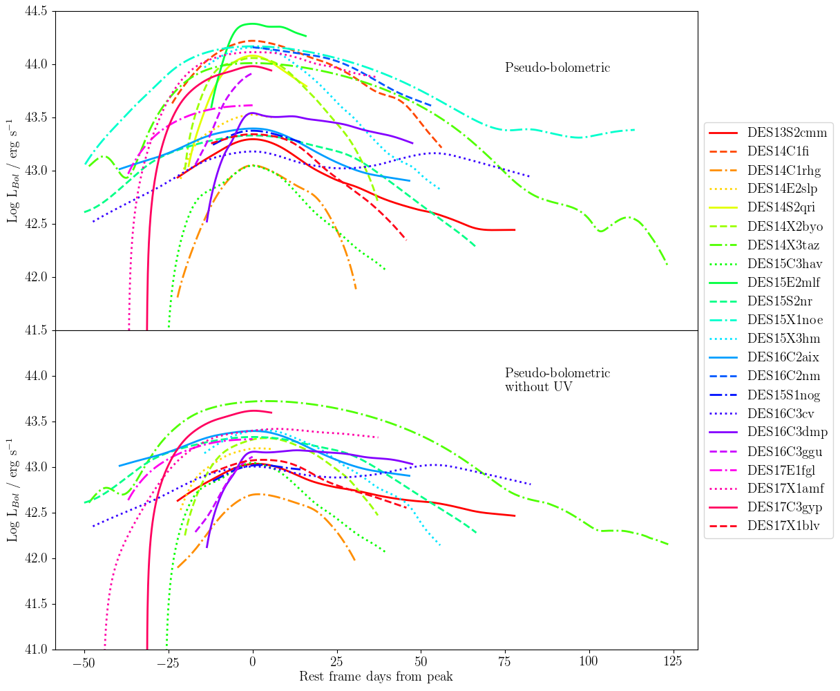
Figure 8: Top: The pseudo-bolometric light curves of DES SLSNe constructed through trapezoidal integration of the $g,r,i,z$ photometry and applying a bolometric correction redwards of the most red observed band to 25000Å. The large range in apparent peak energies, spanning almost 2 dex, could reflect a large spread in initial explosion energies, or imply an efficiency factor in the transferring the initial explosion energy to the SN. Bottom: Pseudo-bolometric light curves with a consistent blue cut-off above $\sim$3800Å. We still see a considerable dispersion in radiated energies when considering similar wavelength ranges in the pseudo-bolometric light curves.

We determine the pseudo-bolometric lightcurves of the SLSNe via trapezoidal integration of the flux in each band at every epoch to obtain a lower limit on the total emitted flux, applying a small red bolometric correction from integration of the best fitting modified black body curve redwards of the most red observed band to 25,000Å. Whilst this correction is typically small ($\sim 0.1$ per cent around peak for most objects), this contribution can become more significant ($\sim 1$ per cent) at late times when the photosphere is cooler. This approach does loose information in the UV, whose contribution to the SED is more significant at early times. However, the rest frame wavelength range probed by the DES photometry does probe the near-UV for the vast majority of objects in this SLSN sample, allowing us to better encapsulate the bolometric behaviour of these events at early times. We present the pseudo-bolometric light curves in the upper panel of Fig. 8.

The large observed spread in peak energies of the DES SLSNe is reinforced within Fig 8, where we observe an apparent $\sim 2$ dex spread in pseudo-bolometric peak flux. This range of peak pseudo-bolometric fluxes approaches much lower energies than has been observed within other SLSN samples (De Cia et al., 2018; Lunnan et al., 2018), with several events peaking at $\lesssim 10^{43}$ erg s^-1, comparable to the peak energies achieved by SNe Ia. This spread in peak luminosities between $\sim 10^{43}$ erg s^-1 and $\sim 10^{44}$ erg s^-1 could be a result of a very flexible progenitor set up (for instance, energy injection from magnetars with a range intrinsic properties), or a reflection of multiple energy sources producing these spectroscopically similar transients.

Given the high-redshift of many objects within our sample, it is possible that the observed spread we see in integrated luminosities is a result of the higher UV contributions from these more distant SLSNe, given the redshift-dependent wavelength range being probed. We therefore present pseudo-bolometric lightcurves with a consistent blue cut-off above $\sim$3800Å(the bluest wavelength probed by the DES observations for the lowest redshift SN in our sample) in the lower panel of Fig. 8, such that we are comparing a similar wavelength range over the entire sample. To avoid excessive extrapolation, we only include objects z$\textless\sim$1.2 in this comparison. As expected, as the UV dominates the SEDs of SLSNe (particularly at early times), we observe a more diminished range of energies here. However, we still observe a broad range in radiated luminosities of $\sim$1 dex, which still implies some range in explosion properties.

Both sets of pseudo-bolometric light curves also highlight the diversity in rise and decline time behaviours within the sample. Several objects at higher redshift ($z>0.4$) rise much more swiftly than the $\sim 20--30$ day rest-frame time identified as a ‘typical characteristic’ of other literature SLSNe.

It is possible that this broad range of physical characteristics could be encapsulated within the framework of a magnetar injection model. This model is capable of producing a broad range of light curve forms, given its dependency upon multiple parameters (including the mass and opacity of the ejected material, which naturally alter the diffusion time of photons through the ejecta). We explore the magnetar model in more detail in the following section.

4.2 The Magnetar Model

The spin-down of a magnetar has been popularly invoked as the underlying energy source of SLSNe within the literature (e.g. Kasen & Bildsten, 2010; Woosley, 2010; Dessart et al., 2012; Inserra et al., 2013; Nicholl et al., 2013; Nicholl et al., 2017b), which given its inherent flexibility, is capable of fitting a wide range of SLSN light curves. Indeed, it has previously been shown that the magnetar model provides a good fit to the main peaks of DES13S2cmm and DES14X3taz (Papadopoulos2015;Smith2016). Given the large diversity in light curve shapes present within the DES SLSNe, we next test the capabilities of the magnetar model against the whole sample.

We fit the magnetar model of Inserra et al. (2013) to our interpolated quasi-bolometric light curves, whose luminosity has the functional form (under the assumption of complete deposition of the magnetar energy into the expanding ejecta) of

$$L_{\mathrm{SN}}\left(t\right)=e^{-(t/\tau_{\mathrm{m}})^{2}}\\ 2\int_{0}^{t/\tau_{\mathrm{m}}}\left(\int 4.9\times 10^{46}\left(\frac{B}{10^{14}~{}\mathrm{G}}\right)^{2}\left(\frac{P}{\mathrm{ms}}\right)^{-4}\frac{1}{(1+t/\tau_{\mathrm{p}})^{2}}\right)\\ e^{(t^{\prime}/\tau_{\mathrm{m}})^{2}}\frac{dt^{\prime}}{\tau_{\mathrm{m}}}\mathrm{~{}erg~{}s^{-1}},$$ (3)

where $B$ and $P$ are the magnetic field strength and period of the magnetar respectively, $\tau_{\mathrm{p}}$ is the spin down timescale of the magnetar, and $\tau_{\mathrm{m}}$ is the diffusion timescale, which under the assumption of uniform ejecta density, can be expressed in terms of the mass, $M_{\mathrm{ej}}$, opacity, $\kappa$, and kinetic energy, $E_{\mathrm{k}}$ of the ejecta

$$\tau_{\mathrm{m}}=1.05(\beta c)^{-0.5}\kappa^{0.5}M_{\mathrm{ej}}^{0.75}E_{\mathrm{k}}^{-0.25}\mathrm{~{}s},$$

where $\beta$ represents a normalisation constant, commonly taken to be 13.7 (Arnett, 1982). Following Inserra et al. (2013), we assume an opacity of $\kappa=0.1~{}\mathrm{cm}^{2}\mathrm{g}^{-1}$ (consistent with hydrogen-free ejecta).

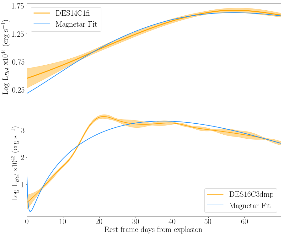
Figure 9: Example magnetar fits (blue lines) quasi-bolometric light curves of DES14C1fi and DES16C3dmp (orange lines). Both fits yield physical values to the magnetar fit parameters, and in some cases provide plausible replications of the bolometric light curves of the DES SLSNe (such as DES14C1fi). However others fair less well upon closer inspection, where the magnetar model is unable to encapsulate the unsmooth evolution of the quasi-bolometric light curve (e.g. DES16C3dmp).

Due to temporal edge effects, some of the DES objects lack the light curve coverage required for a fair assessment of the magnetar model against their bolometric light curves. We therefore introduce a small time step as an additional fit parameter in Equation 3, in which we allow the start date of the SN to vary between $-10$ and $+10$ days to the start of the bolometric light curve. The best fitting magnetar properties are given for each SLSN with Table LABEL:tab:slsnproperties. Whilst this model is able to fit a large fraction of the DES SLSN light curves, visual inspection of many of the fits reveals cases in which the smooth evolution of the magnetar model alone is unable to fully account for the wiggly evolution of the bolometric light curves (for e.g., see Figure 9). Such cases could be a result of artefacts introduced from the GP interpolation, or they could be the result of multiple energy sources powering the light curve (e.g., magnetar + CSM interaction). We discuss this further in Section 7.

Table 3: The derived physical properties from the modified black body and magnetar models applied to the light curves of DES SLSNe.

DES ID	Peak TBB	Peak $R_{\mathrm{BB}}$	$P_{\mathrm{spin}}$	$B$	$M_{\mathrm{ejecta}}$
	($K$)	($cm$)	($ms$)	($10^{14}G$)	($M_{\odot}$)
DES13S2cmm	6.21e+03	7.99e+15	…	…	…
DES14C1fi	1.34e+04	7.99e+15	3.64	3.12	17.32
DES14C1rhg	1.02e+04	2.34e+15	4.95	6.03	3.19
DES14E2slp	8.52e+03	5.75e+15	…	…	…
DES14S2qri	1.054e+04	7.99e+15	4.95	6.03	3.19
DES14X2byo	1.02e+04	7.99e+15	5.88	4.99	3.87
DES14X3taz	1.06e+04	7.99e+15	5.30	2.94	19.66
DES15C3hav	9.30e+03	2.78e+15	…	…	…
DES15E2mlf	1.81e+04	8.00e+15	5.60	2.68	1.10
DES15S2nr	8.85e+03	3.57e+15	10.52	12.47	6.17
DES15X1noe	1.13e+04	7.99e+15	7.45	2.36	1.15
DES15X3hm	1.25e+04	7.99e+15	5.63	3.49	4.18
DES16C2aix	8.25e+03	7.99e+15	…	…	…
DES16C2nm	4.03e+03	6.99e+16	…	…	…
DES15S1nog	1.36e+04	2.31e+15	…	…	…
DES16C3cv	4.53e+03	1.22e+16	…	…	…
DES16C3dmp	1.24e+04	3.36e+15	18.27	9.98	0.23
DES16C3ggu	8.82e+03	8.92e+15	4.80	1.05	16.24
DES17E1fgl	7.38e+03	7.34e+15	9.35	3.60	16.99
DES17X1amf	6.75e+03	1.61e+16	5.56	2.22	11.39
DES17C3gyp	1.07e+04	6.45e+15	6.29	2.94	11.57
DES17X1blv	5.87e+03	8.34e+15	…	…	…

5 Pre-peak Bumps

There now exists strong evidence within the literature that the light curves of some SLSNe are multipeaked. Some events have shown signatures of re-brightening at later times, on both significant scales (e.g. iPTF13ehe Yan et al., 2015), or on much more subtle small scales, manifesting as fluctuations within the decline of the main peak (Nicholl et al., 2016; Inserra et al., 2017). A large fraction of SLSNe have exhibited bumps prior to the main peak of the light curve (Leloudas et al., 2012; Nicholl et al., 2015b; Smith et al., 2016; Anderson et al., 2018). Such features are not highly common to the bulk of the SLSN population, but as they may easily fall below the detection limits of shallower surveys, it is unclear whether these signatures are present in all SLSNe. Understanding the nature of these features may provide the key to understanding the pre-explosion configurations of SLSN progenitors. Here we focus upon the presence of precursory peaks within the DES SLSN light curves.

Whilst the presence of bumps before the main peak of some SLSN light curves are well documented within the literature (Leloudas et al., 2015; Nicholl et al., 2015b), the precise nature of these bumps remains uncertain. Smith et al. (2016) highlighted the pre-peak bump observed within the light curve of DES14X3taz, being detected simultaneously in the DES $g,r,i,z$ bands 20 days prior to the rise of the main peak. Modelling of this bump favoured scenarios involving the shock cooling of an extended CSM located at $\sim 400R_{\odot}$ from the progenitor. To date, this remains the best physically constrained SLSN pre-max bump.

The shock cooling models of Piro (2015) are highly dependant upon three parameters; the mass and radius of the circumstellar envelope ($M_{\mathrm{e}}$ and $R_{\mathrm{e}}$), and the mass of the core prior to explosion $M_{\mathrm{c}}$ (c.f. Arcavi et al., 2017);

$$L(t)= 8.27\times 10^{42}\Big{(}\frac{\kappa}{0.1\mathrm{~{}g~{}cm^{-2}}}\Big{)}^{-1}\Big{(}\frac{v}{10^{9}\mathrm{~{}cm~{}s^{-1}}}\Big{)}^{2}\Big{(}\frac{R}{10^{13}\mathrm{~{}cm}}\Big{)}$$

$$\times\Big{(}\frac{M_{\mathrm{c}}}{M_{\odot}}\Big{)}^{0.01}\times\exp\left[-4.135\times 10^{-11}\right.$$

$$\left.\times t\bigg{(}t\Big{(}\frac{v}{10^{9}\mathrm{~{}cm~{}s^{-1}}}\Big{)}+2\times 10^{4}\Big{(}\frac{R}{10^{13}\mathrm{~{}cm}}\Big{)}\bigg{)}\right.$$

$$\left.\times\Big{(}\frac{\kappa}{0.1\mathrm{~{}g~{}cm^{-2}}}\Big{)}^{-1}\Big{(}\frac{M_{\mathrm{c}}}{M_{\odot}}\Big{)}^{0.01}\Big{(}\frac{M_{\mathrm{e}}}{0.01M_{\odot}}\Big{)}^{-1}\right]\mathrm{erg~{}s^{-1}.}$$ (4)

where $\kappa$ is the opacity of the CSM and $v$ is the expansion velocity of the shock breakout.

The degenerate nature of some of these parameters makes disentangling them for individual events complex, assuming that they all result from the same physical mechanisms. However, the bumps identified so far within the literature (with observations over the entire duration of the bump) appear to be of similar longevity, lasting around $\sim$10-20 days in the rest frame (Leloudas et al., 2012; Nicholl et al., 2015b; Smith et al., 2016), although with a spread in peak luminosities of $\sim$0.5 mag. If all SLSN bumps are the result of shock cooling from an extended circumstellar envelope then a similarity in bump duration may perhaps be indicative of very similar diffusion timescales, such that the combination of envelope mass and radius results in photons escaping the surrounding envelope over approximately the same time for all SLSN bumps.

However, the model of Piro (2015) used to model the bump of DES14X3taz is best constrained using multiband photometric observations, which few SLSNe within the literature possess. Fortunately the multiband photometry of the DES SLSNe presented here therefore offers the opportunity to test for the presence of similar ‘DES14X3taz-like’  bumps within the pre-peak data.

Given the pliability of the Piro (2015) model in its capacity to replicate bumps over a variety of peak luminosities and durations, we test for the presence of bumps under the assumption that all bumps can be described by the model of Piro (2015) and possess similar properties to those which have been documented within the literature.

We therefore take the values of $M_{\mathrm{e}}$ and $R_{\mathrm{e}}$ as determined in Smith et al. (2016) as constant, such that we can place constraints upon the likely range of $M_{\mathrm{c}}$ that may be observed. $M_{\mathrm{c}}$ determines the efficiency of energy transfer from the explosion to the surrounding envelope, such that the change in SN energy with core mass becomes $\frac{E_{\mathrm{SN}}^{\prime}}{E_{\mathrm{SN}}}=\left(\frac{M_{\mathrm{c}}^{\prime}}{M_{\mathrm{c}}}\right)^{0.7}$, and thus is capable of changing the luminosity of the event. We find a core mass of 10.7$\pm$0.4$M_{\odot}$ for DES14X3taz. In Fig. 10 we show the corresponding range of peak bump luminosities (and observed DES $g,r,i,z$ fluxes) which may be generated using this scenario to match the observed spread in peak-bump $g$-band luminosities observed within the literature (e.g. Figure 4 of Smith et al., 2016).

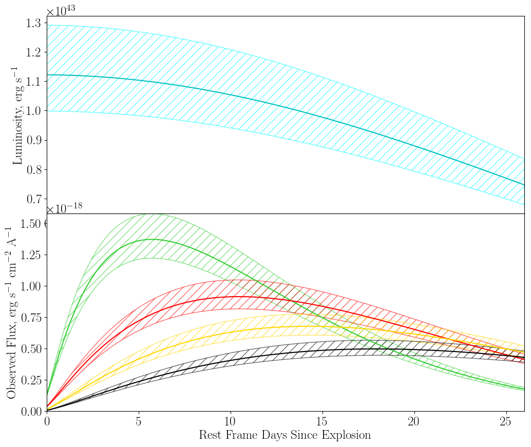
Figure 10: The shock outbreak into an extended CSM model of Piro 2015, for which the mass and radius of the extended material have been fixed to the values found by Smith et al. 2016. We visualise the observed range of peak luminosities and corresponding observable fluxes in the DES filters for this physical scenario over a 5$\sigma$ range for a bump at the redshift of DES14X3taz ($z=0.608$). This basic model is scaled to the redshift of each SLSN in the DES sample used within an iterative Monte Carlo search of the pre-peak data for detections.

We then use this model to search for ‘X3taz-like’ bumps within the DES SLSN data. To do this, we perform Monte Carlo simulations of SLSN bumps within the parameter space of DES14X3taz. Every realisation is then subtracted from the available pre-peak DECam photometry, moving the realised-model iteratively through the data out to $-60$ rest-frame days from the main SN peak. The resulting residuals are then analysed for any $\geq$ 3$\sigma$ detections in each band, with the requisite of that detections are found in a minimum of two or more bands at any epoch. For each event we are therefore able to determine a detection confidence from the ratio of detections to bump-realisations, which thus becomes the probability of having detected an ‘X3taz-like’ for each transient.

Of the DES SLSNe, 14 of the 22 events possess photometry prior to the main SN peak. Using this methodology, we identify significant bump-like signatures for 3 of these SNe, and firmly rule out the presence of bumps for 9/14 SLSNe with sufficient pre-peak data, with non-dectections down to limiting magnitudes of M${}_{g}\sim$-16 for the more local SLSNe within this group ($z\leq 0.5$). In the cases of DES15X1noe and DES15E2mlf, the identification of any bump-like features of DES14X3taz-like magnitude are precluded by the redshifts of these events ($z=1.18,1.86$ respectively). The peculiar case of DES15C3hav is discussed in Section 5.0.1, and we present the rest-frame $g$-band bumps in Figure 11, and the non-detections within Figure 12.

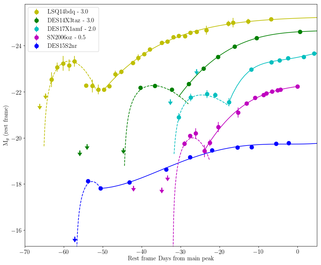
Figure 11: The rest-frame $g$-band lightcurves of DES SLSNe identified with pre-peak bumps (bar DES15C3hav), alongside the bumps of SN2006oz and LSQ14bdq (Leloudas et al., 2012; Nicholl et al., 2015b). Offsets in absolute magnitude have been applied for clarity and 3$\sigma$ limits are given where available. The bumps are fitted with the shock breakout within extended shell model of Piro 2015 (dashed lines), with the main SN peaks fitted with polynomials for clarity (solid lines). In the case of DES17X1amf, its high redshift ($z=0.92$) means the observed $z$-band bump displayed here is a better approximation of its near UV behaviour, rather than its behaviour at blue wavelengths.

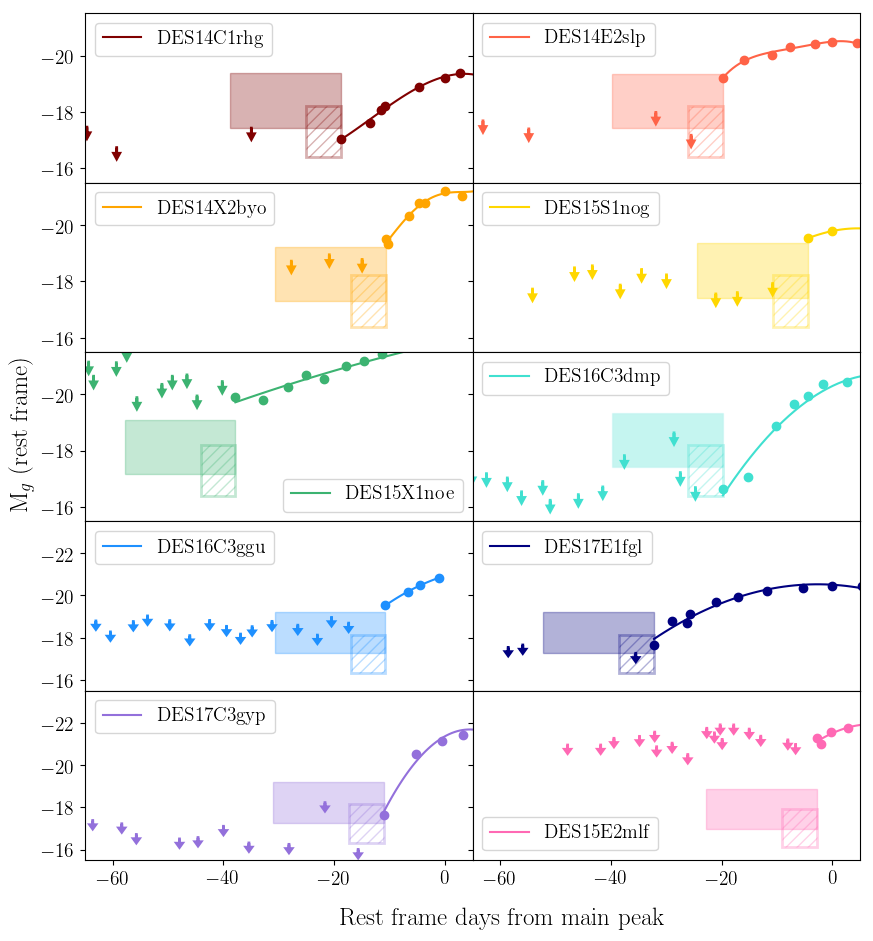
Figure 12: The rest-frame $g$-band light curves of DES SLSNe in which we do not identify a significant bump in the 60 days prior to the start of the main SN light curve. We show the 3$\sigma$ limits for each SN and mark the parameter space in which we would have expected to observe the peak of both a ‘X3taz-like’ and an ‘S2nr-like’ bump in the rest-frame $g$-band (the filled and hatched regions respectively). With the exception of DES15X1noe and DES15E2mlf (whose high redshift precludes the identification of bumps of this magnitude range), we can rule out the presence of an ‘X3taz-like’ bump down to limiting magnitudes of $M\sim-16$ for the more local SLSNe within this group ($z\sim~{}0.5$).

Although identified as having detections consistent with the bump of DES14X3taz, from a wide range of bump durations introduced with the additional DES bumps (in particular, the rapid bump of DES15S2nr), it is clear that the bumps presented within Figure 11 are not all best described by the parameters of DES14X3taz under the Piro (2015) model.

The identity of pre-peak bumps is still unclear. If still powered in a similar manner, the range in durations and luminosities could simply reflect a wider range in pre-explosion set-ups amongst SLSN progenitors, which may be captured within the flexibility of the shock outbreak model. However, other attempts to model bumps have provided equally plausible answers to the origin of SLSN bumps; for instance Margalit et al. (2018) have shown that within the constructs of models involving misalignment between a weak jet and the magnetic dipole of the magnetar powering it, the bump of LSQ14bdq can be explained by a mildly relativistic wind driven from the interface between a jet and the ejecta walls. The precise nature of SLSN bumps is unlikely to be solved without the addition of spectroscopic information. To date, only the potential candidate spectrum obtained during a bump epoch is that of SN2017egm (Xiang et al., 2017; Nicholl et al., 2017a), where an early UV excess is detected within Gaia data, though falling below detection limits in the optical (Bose et al., 2018). The similarity of this spectrum to SLSN spectra near peak may cast doubt upon its identification as a true bump spectrum.

On the other hand, the confirmation of bump-less SLSNe within the DES data is also significant. A combination of poor cadence and shallow photometric limits have not conclusively ruled out the possibility that bumps are ubiquitous in the light curves of SLSN-I (Nicholl & Smartt, 2016). Here the deep, cadenced photometry of DES has provided the limits necessary to rule out the presence of ‘X3taz-like’ bumps within the pre-peak data.

5.0.1 The unusual red ‘bump’of DES15C3hav

The Monte Carlo modelling to search for superluminous bumps also identified an early feature within the pre-peak data of DES15C3hav. Visual inspection of this feature proved it to be exceptionally red for an event at $z=0.376$ when compared to the colour of the main light curve and compared to other SLSN bumps. We observe clear detections within $i$ and $z$ bands, and some partial decline in the $r$ band at later times.

Although this red-feature, shown in Figure 13, rises and declines on approximately the same timescale as a SLSN bump, it is $\sim 2$ magnitudes fainter than the faintest bump identified within our sample, peaking at $M=-16.5$. When fit with a standard black body, it has an estimated black body temperature of $\sim$6000K. This red feature is strikingly different when compared to ‘typical’ SLSN bumps (both here and within the literature), which are blue and hot (Nicholl et al., 2015b; Smith et al., 2016). It is even more unusual when the blueness of the main peak is also considered.

It is possible that this feature is a normal SLSN bump, where the progenitor is surrounded by a shell of high opacity material which is subsequently destroyed during the shock breakout. Under this hypothesis, some properties of the DES15C3hav features could be explained, for instance, the late appearance of $r$-band flux could represent a change in opacity through which bluer light can begin to escape the surrounding shell. To test whether this feature could be described within the framework of the Piro (2015) model, we overlay the bump of DES15C3hav with the Piro (2015) fit to DES14X3taz. We attempt to account for the lack of bluer light during this bump phase by including A_V=3 magnitudes of additional extinction, passing this through the extinction laws of Cardelli et al. (1989) to determine the extinction in the DES bands, and plot the resulting bump within Figure 13. Visually, this provides a poor match to the observed $r,i,z$-band behaviour of the bump of DES15C3hav, although it is sufficient to place the $g$-band light below the detection limits reached with DECam. However, its failure to encapsulate the observed lightcurve in other optical bands makes it unlikely this red feature is a product of shock breakout.

The slow evolution and colour of this red feature are comparable to the ‘plateau’ observed within the pre-maximum data of the more local SLSN, SN2018bsz (Anderson et al., 2018). The slow rising plateau of SN2018bsz, which endures for $>$26 days before the commencement of a more rapid rise to peak, was also found to be extremely red in colour, with a black body temperature of 6700K (Anderson et al., 2018). There are some similarities in the early time behaviour of this SN and DES15C3hav. Although the bump of DES15C3hav is redder (approximate restframe $u-g$ $>$0.59) and so fits a slightly cooler black body, the overall slow evolution and red colour mark these two events as distinct from other pre-peak bump events.

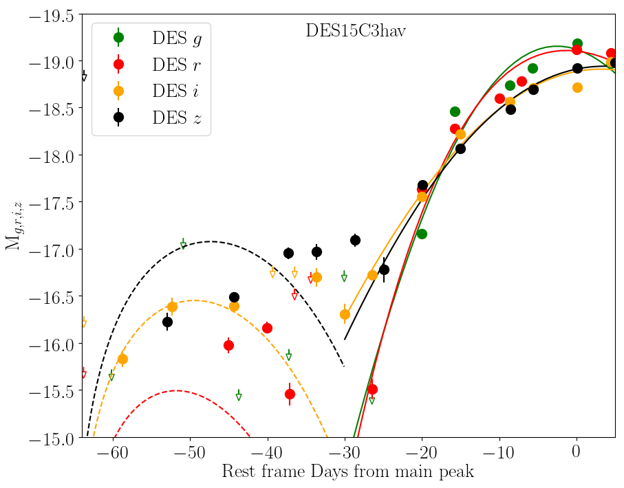
Figure 13: The unusual red bump of DES15C3hav identified at $\sim$50 days prior to the main peak of the transient as seen in the DES $g,r,i,z$ bands. The main peak of the SN in each band is fitted with a polynomial for clarity (solid lines), and 3$\sigma$ limits for each band are also shown. The dashed lines show the expected lightcurve of an ‘X3taz-like’  bump with $\sim$3 magnitudes of additional reddening introduced. This arbitrary inclusion of additional extinction fails to fully capture the behaviour of the bump of DES15C3hav, and requires more detailed modelling to describe its behaviour.

6 Host Galaxies

The host galaxy environments of SLSNe have played an important role in understanding their progenitor origins. Several collective studies have shown that SLSN-I in particular exhibit a strong preference for faint host galaxies with low stellar masses and little star formation (Neill et al., 2011; Lunnan et al., 2014, 2015; Angus et al., 2016; Perley et al., 2016) and generally sub-solar metallicities (Perley et al., 2016; Schulze et al., 2018; Chen et al., 2017a). These features common to the vast majority of SLSN host galaxies all heavily imply progenitors which are young and relatively massive (M$\geq$20M_⊙).

If SLSNe are preferentially produced in low-metallicity environments, as we observe at low redshift, then one may expect to see an evolution of host galaxy properties with redshift, as at higher redshift, galaxies are typically less metal enriched for a given stellar mass (as a result of a less chemically enriched early Universe, leading to an evolving mass-metallicity relationship, Zahid et al., 2014; Ma et al., 2016). The broad redshift range of the DES SLSNe sample allows us to test for the evolution of host properties out to $z\approx 2$.

We perform deep images stacks using images from the five-year DES-SN survey which have been selected such that they contain no SN light and exclude any taken under sub-optimal seeing and atmospheric conditions (Wiseman et al. in prep.). This deep imaging allows us to detect the presence of host galaxy light down to limits of $m\sim 25.5$–26.5 in the shallow and deep fields respectively. To avoid ambiguity in the case of multiple galaxies within the proximity of the SN, we consider the normalized elliptical radius of the galaxy in the direction of the SN (‘directional light radius’, DLR Sullivan et al. 2006; Gupta et al. 2016) of each galaxy. Hosts are identified through minimization of this DLR value. As per Gupta et al. (2016), SNe are marked as ‘hostless’ if the galaxies within the immediate environment have a DLR of $>4$, as this value minimises both the number of hostless events and the number of events with host confusion (Wiseman et al. in prep.).

We identify 16 host galaxies within the stacked images, and find no evidence of host galaxy light in $g,r,i,z$ for 6 of the SLSNe. The fraction of undetected hosts is similar to that seen within PanSTARRS (without the aid of deep HST imaging, Lunnan et al., 2013), although considerably greater than that seen within shallower surveys such as PTF (Perley et al., 2016). Host galaxy stamps are presented within Fig. 14 and their photometry is provided within Table  LABEL:tab:slsnhosts.

Table 4: Photometry of the host galaxies of the DES SLSNe within their stacked $g,r,i,z$ band imaging. Where no host galaxy was detected, 3$\sigma$ limiting magnitudes are provided.

DES ID	mg	mr	mi	mz
DES13S2cmm	23.92 $\pm$ 0.05	23.31$\pm$ 0.04	22.98 $\pm$ 0.03	23.10 $\pm$ 0.05
DES14C1fi	24.52 $\pm$ 0.05	24.37$\pm$ 0.06	24.21 $\pm$ 0.08	23.52 $\pm$ 0.05
DES14C1rhg	$\textgreater$27.17	$\textgreater$26.63	$\textgreater$ 25.37	$\textgreater$25.66
DES14E2slp	$\textgreater$26.99	$\textgreater$25.51	$\textgreater$ 25.04	$\textgreater$25.69
DES14S2qri	$\textgreater$26.75	$\textgreater$26.37	$\textgreater$ 25.97	$\textgreater$26.26
DES14X2byo	$\textgreater$25.93	$\textgreater$25.49	$\textgreater$ 25.58	$\textgreater$25.58
DES14X3taz	25.41 $\pm$ 0.09	24.69 $\pm$ 0.04	24.39 $\pm$ 0.05	24.40 $\pm$ 0.05
DES15C3hav	24.60 $\pm$ 0.03	24.13 $\pm$ 0.01	24.10 $\pm$ 0.02	23.88 $\pm$ 0.02
DES15E2mlf	23.35 $\pm$ 0.02	23.41 $\pm$ 0.02	23.28 $\pm$ 0.03	23.43 $\pm$ 0.05
DES15S1nog	23.33 $\pm$ 0.03	22.54 $\pm$ 0.01	22.16 $\pm$ 0.02	22.06 $\pm$ 0.02
DES15S2nr	23.64 $\pm$ 0.07	23.12 $\pm$ 0.06	22.71 $\pm$ 0.05	22.17 $\pm$ 0.03
DES15X1noe	23.93 $\pm$ 0.04	23.80 $\pm$ 0.04	23.41 $\pm$ 0.04	23.44 $\pm$ 0.05
DES15X3hm	$\textgreater$26.67	$\textgreater$26.28	$\textgreater$25.36	$\textgreater$25.63
DES16C2aix	24.69 $\pm$ 0.07	24.49 $\pm$ 0.07	24.37 $\pm$ 0.09	24.11 $\pm$ 0.09
DES16C2nm	25.31 $\pm$ 0.10	25.08 $\pm$ 0.12	24.94 $\pm$ 0.13	25.45 $\pm$ 0.25
DES16C3cv	$\textgreater$ 26.46	$\textgreater$26.28	$\textgreater$25.94	$\textgreater$25.87
DES16C3dmp	22.26 $\pm$ 0.01	21.55 $\pm$ 0.01	21.29 $\pm$ 0.01	21.22 $\pm$ 0.01
DES16C3ggu	25.21 $\pm$ 0.06	25.19 $\pm$ 0.06	24.78 $\pm$ 0.05	24.49 $\pm$ 0.05
DES17C3gyp	29.17 $\pm$ 2.10	26.85 $\pm$ 0.24	26.62 $\pm$ 0.12	26.29 $\pm$ 0.11
DES17E1fgl	23.29 $\pm$ 0.02	23.06 $\pm$ 0.03	22.64 $\pm$ 0.02	22.86 $\pm$ 0.03
DES17X1amf	26.79 $\pm$ 0.28	27.09 $\pm$ 0.43	26.44 $\pm$ 0.32	25.76 $\pm$ 0.14
DES17X1blv	25.10 $\pm$ 0.13	25.42 $\pm$ 0.20	24.40 $\pm$ 0.11	24.13 $\pm$ 0.10

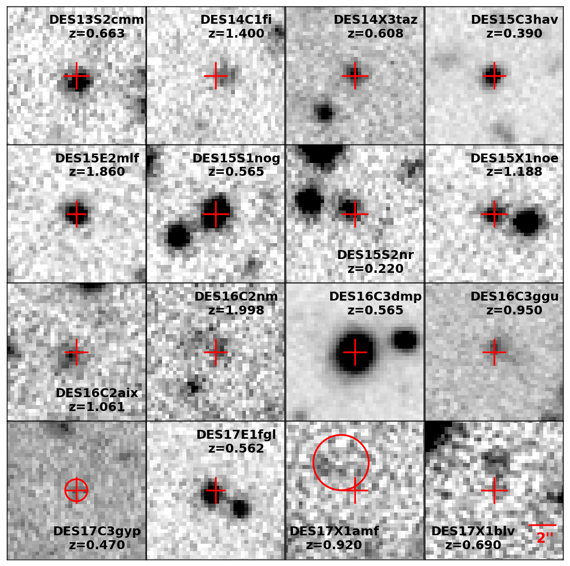
Figure 14: The stacked $r-$band imaging of the DES SLSN hosts. All images are 10″$\times$ 10″. Red crosses mark the location of the SN, and circles mark the loactions of fainter host galaxies where they fall within the limits of our imaging (but are still clearly detected within sextractor). We identify six events in the sample as being hostless down to the limits of our imaging; DES14C1rhg, DES14E2slp, DES14S2qri, DES14X2byo, DES15X3hm and DES16C3cv.

We use sextractor (Bertin & Arnouts, 1996) to determine the mag_auto host galaxy magnitudes in $g,r,i~{}\&z$ bands. We compute the host galaxy stellar masses using the z-peg photometric-redshift software (Le Borgne & Rocca-Volmerange, 2002), which uses the stellar population templates of pégase.2 (Fioc & Rocca-Volmerange, 1997). We assume assume a Kroupa (2002) initial mass function and fix the redshift of each event as reported in Table 1.

Fig. 15 shows the distribution of derived stellar masses, alongside the distribution when broken up into redshift bins of $z<0.6$, 0.6$<z<$1.0 and 1.0$<z<$2.0 (chosen such that we have approximately equal numbers of SNe per redshift bin). Overall, the stellar masses for the DES SLSNe are in accordance with those derived for other SLSN-I hosts, although we observe very little evolution of the mass function with redshift within our relatively small sample of hosts. Whilst visually there may be some slight evolution between intermediate to high-redshift, and is also statistically significant (a Kolmogorov-Smirnov test between the two samples yields a p-value of 0.02), this may be skewed by the small number of objects in each redshift bin. This potential evolution towards higher stellar masses at higher reshift would be consistent with the results of Schulze et al. (2018), whose study of the properties of a larger sample of SLSN host galaxies find a redshift evolution of stellar mass consistent with the general cosmic evolution of starforming galaxies. Such behaviour is consistent with the evolution of the mass-metallicity relationship of field galaxies, supporting the notion of a metallicity bias in SLSN progenitor production.

However, the prerequisite for a faint host galaxy before targeting a candidate for spectroscopic followup may heavily bias our host galaxy results, particularly at low redshifts. We discuss this further within Section 7.3.

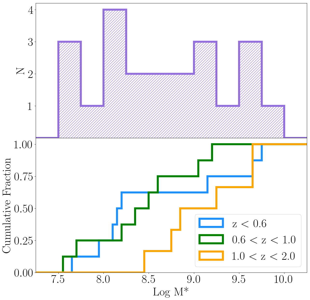
Figure 15: Top: The host galaxy masses of the DES SLSN sample determined using z-peg. Bottom: The mass function broken down into redshift bins of $z<$0.6, 0.6$<z<$1.0 and 1.0$<z<$2.0. There is arguably some evolution between the intermediate and high redshift bins, although small number statistics makes this tenuous.

The properties of the host environment may also impact the properties of the resulting SNe. Such correlations are well established in other SNe classes – for instance, SNe Ia in passive host galaxies are typically lower luminosity events with narrower, faster light curves (e.g., Hamuy et al., 1996; Riess et al., 1999). Other studies of SLSN environments have found tentative relations between the host galaxy enrichment and the derived properties of a magnetar spin-down fit to the bolometric light curve (Chen et al., 2017a).

We test for dependencies of the DES SLSN light curve properties with host galaxy mass. Whilst we find no significant correlation between host stellar mass and SN rise time, decline time, or colour, we do see a tentative negative correlation between stellar mass and the decline in the 4000 Å band between peak and 30 days, which we show in Figure 16. This suggests that we observe more quickly evolving (i.e., redder at 30 days post-peak) events within lower mass host galaxies. Whilst we lack the sample size to draw more conclusions, this could be indicative of metallicity effects upon the progenitor stars; for instance, metal poor progenitors will have more optically thin ejecta, allowing energy to escape more easily, or perhaps within the paradigm of the relation between host metallicity and magnetar spin of Chen et al. (2017a), a more rapidly spinning magnetar (for a given magnetic field strength) releases its energy much more quickly, resulting in a redder SN.

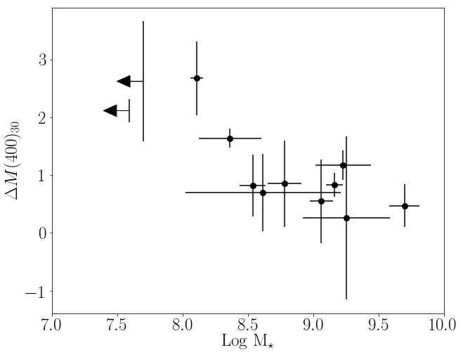
Figure 16: The apparent correlation between the evolution of DES SLSNe in the 4000Å band between peak and 30 days and their host galaxy stellar masses. Although small numbers dominates our ability to draw firm conclusions, this relation could be indicative of stellar mass (and so metallicity) effects upon SLSN evolution.

7 Discussion

7.1 SLSN sample

The definition of a SLSN has undergone many changes over the relatively short period since their discovery. The application of a luminosity threshold to select these events has for some time been found insufficient, occasionally leading to the inclusion of non-SLSN events such as tidal disruption events (TDEs, e.g. ASASSN-15lh Leloudas et al. 2016), and SN Ia-CSM events (whose interaction bolsters both luminosity and duration of the transient, Silverman et al., 2013), resulting in an contaminated and poorly defined literature sample. Whilst homogeneously selected samples of SLSNe have begun to highlight a wider spread in their photometric properties (Lunnan et al., 2018; De Cia et al., 2018), they are still characterised as being generally more luminous than SNe Ia and CCSN events, and with slow light curve evolution.

The sample of SLSNe within DES are all spectroscopically similar to other SLSNe within the literature; however, there exists a large amount of internal diversity within their light curves. Our distribution of peak luminosities spans almost four magnitudes, nearly 0.5 mag fainter than observed previously within the literature. De Cia et al. (2018) have shown that, based upon the sample of SLSNe, SNe Ic-BL and SNe Ibc observed within PTF, the volume-corrected distribution in peak luminosities for these transients shows no evidence that SLSNe are a separate population of events. The volume-weighted luminosity function presented here supports this, and broadens the range of peak luminosity space occupied by SLSNe. Such a continuous distribution could indicate similarities in the underlying explosion mechanisms, with some variation in progenitor set-up which could lead to the production of a brighter or fainter transient accordingly.

Despite the somewhat limited light curve coverage resulting from the restricted length of the DES observing seasons, within the DES sample we see a wide range of rise times spanning a factor of $\sim 4$, with some objects rising to peak bolometric luminosity in just 12 days in the rest frame (see DES15E2mlf, DES16C3dmp), whilst others taking nearly 50 days (DES15X1noe). A similarly broad spread is observed in decline timescales.

A variety of general light curve properties were observed in both PTF and PANSTARRS samples. However, the well-constrained photometry of the DES survey reveals additional peculiarities, with many small-scale re-brightening events such as those identified by Inserra et al. (2017), and the double-peaked re-brightening event of DES16C3cv, where the quasi-bolometric luminosity of the secondary peak is comparable to the brightness of the main peak. Whilst in isolated events, such deviations from a smooth light curve evolution may be less surprising, the fraction of SLSNe from DES which exhibit ‘atypical’ behaviour is extremely high. It may be that this behaviour is common to all SLSNe, and has simply been highlighted by a combination of better photometric constraints and a higher redshift sample (where time-dilation allows these features to be more easily identified), as we begin to see deviations from ‘normal’ behaviour in deeper photometric surveys (cf. Lunnan et al., 2018).

The diversity in light curve properties has implications for the physical interpretation of SLSNe too. The application of a modified black body model has shown a peak temperature range between $\sim 4000$ and $18000$ K, whilst in bolometric space this equates to a spread of $\sim 1.5$ dex in radiated energy. Magnetar energy injection has been popularly invoked to explain the observed luminosities and decline timescales of many SLSNe (see Kasen & Bildsten, 2010; Nicholl et al., 2013; Inserra et al., 2013; Nicholl et al., 2017a; Dessart, 2018). Whilst capable of replicating a wide range of transient lightcurves, this model presents a very smooth light curve profile, which by itself fails to capture the small scale variations seen within some light curves. We have shown that magnetars are incapable of describing some of the DES SLSNe, where the smooth evolution of the model cannot replicate the unusual light curves of some objects.

There is a growing school of thought that magnetar injection cannot solely be responsible for the production of SLSNe, and may in fact be one of multiple energy production mechanisms that power the main light curve (Wang et al., 2016). For instance, the addition of CSM interaction would naturally explain bumpy lightcurves at late times, where the expanding ejecta reaches more distant shells of discarded stellar envelope as it moves outwards (Inserra et al., 2018d). The flexibility of the CSM model too, has appeal in describing why the features are not ubiquitous to all SLSN light curves, as a low mass, low-opacity shell may not produce detectable wiggles within the late time light curve.

However, the delayed injection of energy from a central engine, rather than an instantaneous injection of energy at the point of collapse, as most models assume, may provide an explanation for the spread in peak luminosities observed for transients which are similar both spectroscopically and in their photometric evolution (i.e., Fig. 7). A time delay following the collapse allows some of the ejecta to fall back onto the newly formed compact remnant, reducing the ejecta mass and therefore the energy of the outward explosion (see Woosley, 2018). This might explain the distribution of SLSNe within the 4OPS parameter space shown in Fig. 7, as the same physical mechanism causes the SN to evolve as they do, but is capable of producing a broad range in peak energies.

7.2 Bumps

The enigmatic presence of pre-peak bumps within the light curves of some SLSNe-I has been recognised for some time. Their postulated origins vary wildly, from shock breakout into some form of extended stellar envelope or CSM (Piro, 2015; Nicholl et al., 2015b; Smith et al., 2016; Vreeswijk et al., 2017), to signatures of the shock created by the switch-on of a central magnetar at early times (Kasen et al., 2016), to emission from the collision of the SN ejecta with a close orbiting companion star (Moriya et al., 2015). Whatever their underlying physical nature, up unto this point it has been unclear whether these features are present within the light curves of all SLSNe, where some fraction simply sit below the detection limits of their given surveys, or if they are simply not present at all.

The depth of DECam imaging has allowed us to rule out the presence of ‘X3taz-like’ bump-like features (down to the limits of their respective imaging) within the light curves of 10 SLSNe. Furthermore, we have shown that a significant level of diversity (in both duration and luminosity) exists amongst the three bumps which are detected within the early time data.

Under different physical setups, models involving the rapid heating and cooling caused by shock breakout within the progenitor envelopes prior to the main SNe are capable of encapsulating the wide variety of bump shapes observed within the DES sample. Degeneracies between the parameters within this model make it impossible to use any potential similarities in bump properties as hints of underlying progenitor properties, but with the inclusion of the DES sample, we clearly observe a much wider spread in bump properties than initially considered.

Observations of precursory bumps within SN extends to include some much fainter core collapse SNe (c.f. Campana et al., 2006; Soderberg et al., 2008; Arcavi et al., 2011; Taddia et al., 2016; Barbarino et al., 2017; Taddia et al., 2018), but why these events appear to manifest themselves most prominently within the light curves of more luminous supernovae is unclear. Unfortunately the DES dataset does not posses the cadence for more fine tuned models, typically sampling the light curve twice over the bump epoch. The addition of the DES SLSN bumps to the growing sample of observed bumps within the literature does not clarify the question of whether all bumps arise from the same underlying physical mechanism. However, this sample has significantly broadened the range of bump luminosities (which may, like the luminosities of the main peak, form a continuous distribution) and durations, which, if they are of one origin, suggests some flexibility in the allowed initial conditions prior to bump production.

On the other hand, the lack of a pre-peak bump within some SLSN light curves is equally significant. Again, the source of energy production is common to all events, this could point to a variety of progenitor scenarios, in which sometimes the conditions are favourable for the production of a pre-peak bump, and in others less so. We note, that although our Monte-Carlo search revealed no bump prior to the start of the main peak, in some objects (particularly DES14X2byo and DES16C3dmp), we observe a small kink during the rise of the bluer bands in the light curve. It is possible that these small features may represent ‘belated pre-peak shock-cooling bumps’, where the extended material lies further from the progenitor than within a ‘classical’ pre-peak bump (i.e. a ‘14X3taz-like’) whose emission becomes merged with the main peak of the SN. Under a combined emission hypothesis, the appearance of prompt, belated or post-peak wiggles could simply represent CSM interaction across a range of radii from the progenitor.

The red pre-peak feature of DES15C3hav is also intriguing, in particular its contrast in colour and apparent temperature to the main peak of the SN. Our observations rule out the use of a shock breakout model to describe this feature. Anderson et al. (2018) suggest that the red plateau phase prior to the rise of the main peak of SN2018bsz could be explained by the late time injection of magnetar energy following a normal SN-Ibc event, which results in a more luminous SN at peak. This could be applicable to the behaviour of DES15C3hav, although it does not fully account for its strange colour evolution, in particular, the sudden decrease in $r$-band flux towards the end of the bump epoch.

7.3 Selection Biases & Future SLSN Searches

Given its cosmology-orientated science goals, the DES-SN survey is not an untargeted survey, with the spectroscopic follow-up primarily focused upon SN-Ia classification. The spectroscopic followup of our sample was prioritised based upon the ‘known’ properties of SLSN from previous studies – i.e., some combination of light curve and host galaxy properties, in particular for having long observed rise/decline times, and standing out as being several magnitudes brighter than any apparent host. Therefore our SLSN spectroscopic followup is likely to be incomplete.

Under the assumption that these properties are typical of a SLSN, we can roughly estimate our spectroscopic completeness here based upon the highest redshift that we could have confirmed our faintest SLSN out to, which we find to be $z\approx 0.63$. A comprehensive estimate of the number of spectroscopic completeness of DES SLSN followup will be presented within Thomas et al. (in prep.)

However, given the growing diversity in SLSN properties presented both here and within the literature (Lunnan et al., 2018; De Cia et al., 2018), this is likely to be an underestimate. The range of rest frame rise and decline times observed within the spectroscopically confirmed SLSNe in this work suggests that it is possible that our perquisite for a slow rise may result in some missing some fraction of low-$z$ events where the affects of time dilation are reduced, and therefore the SLSN evolves more quickly in the observer frame. However, without a spectroscopic redshift for every transient, the level of bias that this prerequisite introduces is difficult to quantify.

The massive spiral galaxy host to SN2017egm (Nicholl et al., 2017a; Izzo et al., 2018; Chen et al., 2017b) highlights another bias in SLSN followup; although the fraction of SLSN within relatively massive host galaxies remains low, it is unclear whether this is the norm, and if SN2017egm-like events are simply missed by the majority of surveys due to the targeting of transients in fainter hosts. We test this faint-host bias within DES by searching for photometric candidate events which pass our other lightcurve criteria but are located within any host environment (bright or faint), and find that 66 unclassified transients pass this criteria. Given that we triggered spectroscopic follow up of 30 candidates under programmes designed to include SLSN events, this implies a followup completeness of ‘SLSN-like’ events within DES of $\sim 31$ per cent

Within this sample of 66 unclassified transients, we find that 12 meet our faint host criterion for spectroscopic followup. If this sample of candidate events were pure, this suggests that $\sim 81$ per cent of possible SLSN events are missed due to their relatively ‘bright’ host galaxies. Such a heavy bias in spectroscopic followup strategies could have implications for the progenitors SLSNe. Low luminosity, low mass host galaxies have previously been used as evidence for a young, massive population of progenitor stars (Neill et al., 2011; Chen et al., 2013; Lunnan et al., 2014; Angus et al., 2016; Perley et al., 2016). If SLSNe are indeed less localized to such exclusive environments, this widens the potential range of progenitor types significantly.

However, this is highly likely to be an overestimate of the true fraction of missed SLSN events, as low-luminosity AGN outbursts may contaminate the sample, where any underlying variability from the source would likely fall within the noise of the survey, and thus lead to miss classification of the candidate event.

8 Conclusions

We have presented the light curves and classification spectra of 22 SLSNe from Y1-Y5 of DES. Objects in this sample were not initially selected based upon a luminosity cut, but rather based upon their slow light curve evolution, blue colour and faint host environment. They were classified as SLSNe based upon their spectroscopic similarity to other SLSNe identified within the literature, and this sample continues to add to the growing number of homogeneously selected SLSNe from wide-field surveys, although here we present the broadest redshift range yet within a spectroscopic sample, with a median redshift of 0.7 and reaching out to $z\sim 2$. Analysis of the photometric properties of this sample show the following:

• The DES sample significantly extends the range of peak luminosities observed within the SLSN population, with the tail end of the distribution beginning to broach the peak luminosities of SN-Ia ($M\sim-19$).

• We observe a broad spectrum of light curve characteristics (rise/decline times) and a large fraction of SLSNe which present ‘atypical’ behaviour within the main peak of their light curves. This behaviour is difficult to encapsulate within the framework of a magnetar model alone. It is unclear whether this level of diversity is a direct result of multiple energy production mechanisms or a wide variety of progenitor properties.

• We find signatures of pre-peak bumps are present within the light curves of three SLSNe within our sample. The range of bump durations and peak luminosities suggests again some variety in progenitor set-up prior to explosion.

• We identify a particularly red feature prior to the main peak of DES15C3hav, which we are unable to describe under shock breakout models.

• We can confirm the absence of pre-peak bumps within the first 60 days before the main peak within 10 SLSNe down to limits of $M\sim-16$. Although there are one or two cases in which we observe some excess of blue light (blue ‘kinks’) within the rise of the main peak, which may be signatures of a delayed pre-peak bump, the absence of bumps in a large fraction of light curves suggests they are no ubiquitous to all events of this class.

It is clear that a magnitude limit cannot be applied to blindly select SLSNe within a survey. This work highlights the importance of multiband information in understanding their behaviour. In future surveys, an emphasis upon early-time spectroscopic followup may help to provide a better understanding of the mechanism(s) driving the main peak of the transient, but also of the nature of pre-peak bumps which are present within some SLSNe, and their connection to the main SN event.

Appendix A Appendix

DES ID	Date Obs.	Telescope
		(s)
DES13S2cmm	2013-11-21$\star$	VLT/Xshooter
DES14C1fi	2014-09-21	AAT/AAOmega
	2014-09-24	KECK/LRIS
	2014-10-24	KECK/LRIS
	2014-10-30	AAT/AAOmega
	2014-10-30$\star$	VLT/Xshooter
DES14C1rhg	2014-12-21	AAT/AAOmega
	2014-12-24	AAT/AAOmega
	2014-12-29$\star$	VLT/Xshooter
	2014-12-29	AAT/AAOmega
DES14E2slp	2014-12-29$\star$	VLT/Xshooter
DES14S2qri	2015-01-21$\star$	GTC/OSIRIS
DES14X2byo	2014-10-18	GTC/OSIRIS
	2014-10-23	MMT/Blue Grating Spec.
	2014-10-24$\star$	KECK/LRIS
	2014-10-28	AAT/AAOmega
	2014-11-16	MAGELLAN
	2014-11-16	MAGELLAN
	2014-11-20	AAT/AAOmega
	2014-11-21	AAT/AAOmega
	2015-01-21	GTC/OSIRIS
DES14X3taz	2015-01-26$\star$	GTC/OSIRIS
	2015-02-06	GTC/OSIRIS
DES15C3hav	2015-11-04	VLT/Xshooter
	2015-11-09$\star$	MMT/Blue Grating Spec.
	2015-11-12	AAT/AAOmega
	2015-11-13	AAT/AAOmega
	2015-12-12	AAT/AAOmega
DES15E2mlf	2015-12-06	GEMINI-S/GMOS
	2015-12-12	AAT/AAOmega
	2015-12-14	AAT/AAOmega
	2015-12-15$\star$	GEMINI-S/GMOS
	2016-01-14	GEMINI-S/GMOS
DES15S1nog	2016-02-11$\star$	GTC/OSIRIS
DES15S2nr	2015-09-19	VLT/Xshooter
	2015-09-19	AAT/AAOmega
	2015-09-21	AAT/AAOmega
	2015-10-06	VLT/Xshooter
	2015-10-10$\star$	KECK/LRIS
	2015-10-19	SALT
	2015-10-20	SALT
	2015-11-03	SALT
	2015-11-04	VLT/Xshooter
	2015-11-08	SALT
	2015-12-03	AAT/AAOmega
	2015-12-11	KECK/LRIS
DES15X1noe	2016-01-28$\star$	GTC/OSIRIS
DES15X3hm	2015-09-09$\star$	VLT/Xshooter
	2015-09-16	AAT/AAOmega
	2015-09-17	AAT/AAOmega
	2015-09-19	AAT/AAOmega
DES16C2aix	2016-10-10$\star$	MAGELLAN
	2016-11-03	AAT/AAOmega
	2016-11-26	AAT/AAOmega
	2016-11-28	AAT/AAOmega
	2016-11-29	AAT/AAOmega
DES16C2nm	2016-10-10$\star$	MAGELLAN
	2016-10-23	VLT/Xshooter
	2016-10-24	KECK/LRIS
	2016-10-24	VLT/Xshooter
	2016-11-21	VLT/Xshooter

DES ID	Telescope	Date Obs.
		(s)
DES16C3cv	2016-09-25	VLT/Xshooter
	2016-09-25	AAT/AAOmega
	2016-10-10$\star$	MAGELLAN
	2016-12-27	KECK/LRIS
DES16C3dmp	2016-11-25	AAT/AAOmega
	2016-11-28	AAT/AAOmega
	2016-12-20$\star$	VLT/Xshooter
DES16C3ggu	2017-02-25$\star$	VLT/Xshooter
DES17C3gyp	2018-01-09	SALT
	2018-01-24$\star$	AAT/AAOmega
DES17E1fgl	2017-12-22$\star$	AAT/AAOmega
DES17X1amf	2017-09-22	MAGELLAN
	2017-10-22	AAT/AAOmega
	2017-11-10$\star$	MAGELLAN
	2017-11-19	AAT/AAOmega
	2017-12-23	AAT/AAOmega
DES17X1blv	2017-11-10	MAGELLAN
	2017-11-11$\star$	VLT/Xshooter
	2017-11-19	AAT/AAOmega

Table 5: A $\star$ indictaes the spectrum was used for classification.

Appendix B DES Photometry

Table 6: DECam photometry of DES SLSNe. This is an abbreviated version of this table, shown here for content. The full table can be found in the electronic version of the article.

DES ID	MJD	Phase	Band	Mag	MagErr
DES13S2cmm	56534.28	-16.91	g	23.07	0.04
DES13S2cmm	56534.29	-16.91	r	22.79	0.04
DES13S2cmm	56534.29	-16.90	i	22.88	0.05
DES13S2cmm	56534.29	-16.90	z	22.69	0.05
DES13S2cmm	56538.32	-14.48	g	23.18	0.04
DES13S2cmm	56538.33	-14.48	r	22.60	0.03
DES13S2cmm	56538.33	-14.47	i	22.58	0.04
DES13S2cmm	56538.33	-14.47	z	22.73	0.07
DES13S2cmm	56543.30	-11.49	g	22.92	0.03
DES13S2cmm	56543.30	-11.49	r	22.41	0.03
DES13S2cmm	56543.30	-11.49	i	22.56	0.04
DES13S2cmm	56543.30	-11.48	z	22.45	0.05
		…

References

- Ambikasaran et al. (2014) Ambikasaran S., Foreman-Mackey D., Greengard L., Hogg D. W., O’Neil M., 2014
- Anderson et al. (2018) Anderson J. P., et al., 2018, preprint, (arXiv:1806.10609)
- Angus et al. (2016) Angus C. R., Levan A. J., Perley D. A., Tanvir N. R., Lyman J. D., Stanway E. R., Fruchter A. S., 2016, MNRAS, 458, 84
- Arcavi et al. (2011) Arcavi I., et al., 2011, ApJ, 742, L18
- Arcavi et al. (2017) Arcavi I., et al., 2017, ApJ, 837, L2
- Arnett (1982) Arnett W. D., 1982, ApJ, 253, 785
- Barbarino et al. (2017) Barbarino C., et al., 2017, MNRAS, 471, 2463
- Bernstein et al. (2012) Bernstein J. P., et al., 2012, ApJ, 753, 152
- Bertin & Arnouts (1996) Bertin E., Arnouts S., 1996, A&AS, 117, 393
- Bose et al. (2018) Bose S., et al., 2018, ApJ, 853, 57
- Campana et al. (2006) Campana S., et al., 2006, Nature, 442, 1008
- Cardelli et al. (1989) Cardelli J. A., Clayton G. C., Mathis J. S., 1989, ApJ, 345, 245
- Chen et al. (2013) Chen T.-W., et al., 2013, ApJ, 763, L28
- Chen et al. (2017a) Chen T.-W., Smartt S. J., Yates R. M., Nicholl M., Krühler T., Schady P., Dennefeld M., Inserra C., 2017a, MNRAS, 470, 3566
- Chen et al. (2017b) Chen T.-W., et al., 2017b, ApJ, 849, L4
- Cooke et al. (2012) Cooke J., et al., 2012, Nature, 491, 228
- Dark Energy Survey Collaboration et al. (2016) Dark Energy Survey Collaboration et al., 2016, MNRAS, 460, 1270
- De Cia et al. (2018) De Cia A., et al., 2018, ApJ, 860, 100
- Desai et al. (2012) Desai S., et al., 2012, ApJ, 757, 83
- Dessart (2018) Dessart L., 2018, A&A, 610, L10
- Dessart (2019) Dessart L., 2019, A&A, 621, A141
- Dessart et al. (2012) Dessart L., Hillier D. J., Waldman R., Livne E., Blondin S., 2012, MNRAS, 426, L76
- Dexter & Kasen (2013) Dexter J., Kasen D., 2013, ApJ, 772, 30
- Diehl et al. (2018) Diehl H. T., et al., 2018, in Observatory Operations: Strategies, Processes, and Systems VII. p. 107040D, doi:10.1117/12.2312113
- Fioc & Rocca-Volmerange (1997) Fioc M., Rocca-Volmerange B., 1997, A&A, 326, 950
- Firth et al. (2015) Firth R. E., et al., 2015, MNRAS, 446, 3895
- Flaugher et al. (2015) Flaugher B., et al., 2015, AJ, 150, 150
- Gal-Yam (2012) Gal-Yam A., 2012, Science, 337, 927
- Goldstein et al. (2015) Goldstein D. A., et al., 2015, AJ, 150, 82
- Gupta et al. (2016) Gupta R. R., et al., 2016, AJ, 152, 154
- Hamuy et al. (1996) Hamuy M., Phillips M. M., Suntzeff N. B., Schommer R. A., Maza J., Aviles R., 1996, AJ, 112, 2391
- Howell (2017) Howell D. A., 2017, in Alsabti A., Murdin P., eds, , Handbook of Supernovae. Springer, Cham, pp 431–458
- Howell et al. (2005) Howell D. A., et al., 2005, ApJ, 634, 1190
- Howell et al. (2013) Howell D. A., et al., 2013, ApJ, 779, 98
- Hsiao et al. (2007) Hsiao E. Y., Conley A., Howell D. A., Sullivan M., Pritchet C. J., Carlberg R. G., Nugent P. E., Phillips M. M., 2007, ApJ, 663, 1187
- Inserra & Smartt (2014) Inserra C., Smartt S. J., 2014, ApJ, 796, 87
- Inserra et al. (2013) Inserra C., et al., 2013, ApJ, 770, 128
- Inserra et al. (2017) Inserra C., et al., 2017, MNRAS, 468, 4642
- Inserra et al. (2018a) Inserra C., et al., 2018a, MNRAS, 475, 1046
- Inserra et al. (2018b) Inserra C., et al., 2018b, A&A, 609, A83
- Inserra et al. (2018c) Inserra C., Prajs S., Gutierrez C. P., Angus C., Smith M., Sullivan M., 2018c, ApJ, 854, 175
- Inserra et al. (2018d) Inserra C., Prajs S., Gutierrez C. P., Angus C., Smith M., Sullivan M., 2018d, ApJ, 854, 175
- Izzo et al. (2018) Izzo L., et al., 2018, A&A, 610, A11
- Kasen & Bildsten (2010) Kasen D., Bildsten L., 2010, ApJ, 717, 245
- Kasen et al. (2011) Kasen D., Woosley S. E., Heger A., 2011, ApJ, 734, 102
- Kasen et al. (2016) Kasen D., Metzger B. D., Bildsten L., 2016, ApJ, 821, 36
- Kessler et al. (2015) Kessler R., et al., 2015, AJ, 150, 172
- Kroupa (2002) Kroupa P., 2002, Science, 295, 82
- Le Borgne & Rocca-Volmerange (2002) Le Borgne D., Rocca-Volmerange B., 2002, A&A, 386, 446
- Leloudas et al. (2012) Leloudas G., et al., 2012, A&A, 541, A129
- Leloudas et al. (2015) Leloudas G., et al., 2015, MNRAS, 449, 917
- Leloudas et al. (2016) Leloudas G., et al., 2016, Nature Astronomy, 1, 0002
- Liu et al. (2017) Liu Y.-Q., Modjaz M., Bianco F. B., 2017, ApJ, 845, 85
- Lunnan et al. (2013) Lunnan R., et al., 2013, ApJ, 771, 97
- Lunnan et al. (2014) Lunnan R., et al., 2014, ApJ, 787, 138
- Lunnan et al. (2015) Lunnan R., et al., 2015, ApJ, 804, 90
- Lunnan et al. (2016) Lunnan R., et al., 2016, ApJ, 831, 144
- Lunnan et al. (2018) Lunnan R., et al., 2018, ApJ, 852, 81
- Ma et al. (2016) Ma X., Hopkins P. F., Faucher-Giguère C.-A., Zolman N., Muratov A. L., Kereš D., Quataert E., 2016, MNRAS, 456, 2140
- Margalit et al. (2018) Margalit B., Metzger B. D., Thompson T. A., Nicholl M., Sukhbold T., 2018, MNRAS, 475, 2659
- Mazzali et al. (2016) Mazzali P. A., Sullivan M., Pian E., Greiner J., Kann D. A., 2016, MNRAS, 458, 3455
- McCrum et al. (2015) McCrum M., et al., 2015, MNRAS, 448, 1206
- Metzger et al. (2014) Metzger B. D., Vurm I., Hascoët R., Beloborodov A. M., 2014, MNRAS, 437, 703
- Mohr et al. (2012) Mohr J. J., et al., 2012, in Software and Cyberinfrastructure for Astronomy II. p. 84510D (arXiv:1207.3189), doi:10.1117/12.926785
- Morganson et al. (2018) Morganson E., et al., 2018, PASP, 130, 074501
- Moriya et al. (2015) Moriya T. J., Liu Z.-W., Mackey J., Chen T.-W., Langer N., 2015, A&A, 584, L5
- Moriya et al. (2018) Moriya T. J., et al., 2018, preprint, (arXiv:1801.08240)
- Neill et al. (2011) Neill J. D., et al., 2011, ApJ, 727, 15
- Nicholl & Smartt (2016) Nicholl M., Smartt S. J., 2016, MNRAS, 457, L79
- Nicholl et al. (2013) Nicholl M., et al., 2013, Nature, 502, 346
- Nicholl et al. (2015a) Nicholl M., et al., 2015a, MNRAS, 452, 3869
- Nicholl et al. (2015b) Nicholl M., et al., 2015b, ApJ, 807, L18
- Nicholl et al. (2016) Nicholl M., et al., 2016, ApJ, 826, 39
- Nicholl et al. (2017a) Nicholl M., Berger E., Margutti R., Blanchard P. K., Guillochon J., Leja J., Chornock R., 2017a, ApJ, 845, L8
- Nicholl et al. (2017b) Nicholl M., Guillochon J., Berger E., 2017b, ApJ, 850, 55
- Nicholl et al. (2019) Nicholl M., Berger E., Blanchard P. K., Gomez S., Chornock R., 2019, ApJ, 871, 102
- Ofek et al. (2014) Ofek E. O., et al., 2014, ApJ, 788, 154
- Pan et al. (2017) Pan Y.-C., et al., 2017, MNRAS, 470, 4241
- Papadopoulos et al. (2015) Papadopoulos A., et al., 2015, MNRAS, 449, 1215
- Pastorello et al. (2010) Pastorello A., et al., 2010, ApJ, 724, L16
- Perley et al. (2016) Perley D. A., et al., 2016, ApJ, 830, 13
- Piro (2015) Piro A. L., 2015, ApJ, 808, L51
- Prajs et al. (2016) Prajs S., et al., 2016, MNRAS,
- Quimby et al. (2011) Quimby R. M., et al., 2011, Nature, 474, 487
- Quimby et al. (2013) Quimby R. M., Yuan F., Akerlof C., Wheeler J. C., 2013, MNRAS, 431, 912
- Quimby et al. (2018) Quimby R. M., et al., 2018, ApJ, 855, 2
- Rasmussen & Williams (2006) Rasmussen C. E., Williams C. K. I., 2006, Gaussian Processes for Machine Learning
- Riess et al. (1999) Riess A. G., et al., 1999, AJ, 117, 707
- Sako et al. (2011) Sako M., et al., 2011, ApJ, 738, 162
- Schlafly & Finkbeiner (2011) Schlafly E. F., Finkbeiner D. P., 2011, ApJ, 737, 103
- Schulze et al. (2018) Schulze S., et al., 2018, MNRAS, 473, 1258
- Sevilla et al. (2011) Sevilla I., et al., 2011, preprint, (arXiv:1109.6741)
- Silverman et al. (2013) Silverman J. M., et al., 2013, ApJS, 207, 3
- Smith et al. (2007) Smith N., et al., 2007, ApJ, 666, 1116
- Smith et al. (2016) Smith M., et al., 2016, ApJ, 818, L8
- Smith et al. (2018) Smith M., et al., 2018, ApJ, 854, 37
- Soderberg et al. (2008) Soderberg A. M., et al., 2008, Nature, 453, 469
- Sullivan et al. (2006) Sullivan M., et al., 2006, ApJ, 648, 868
- Taddia et al. (2016) Taddia F., et al., 2016, A&A, 592, A89
- Taddia et al. (2018) Taddia F., et al., 2018, A&A, 609, A106
- The Dark Energy Survey Collaboration (2005) The Dark Energy Survey Collaboration 2005, ArXiv Astrophysics e-prints,
- Vreeswijk et al. (2017) Vreeswijk P. M., et al., 2017, ApJ, 835, 58
- Wang et al. (2016) Wang S. Q., Liu L. D., Dai Z. G., Wang L. J., Wu X. F., 2016, ApJ, 828, 87
- Woosley (2010) Woosley S. E., 2010, ApJ, 719, L204
- Woosley (2018) Woosley S. E., 2018, ApJ, 863, 105
- Xiang et al. (2017) Xiang D., Song H., Wang X., Rui L., Xiao F., Zhang T., Zhang J., 2017, The Astronomer’s Telegram, 10442
- Yan et al. (2015) Yan L., et al., 2015, ApJ, 814, 108
- Yan et al. (2017) Yan L., et al., 2017, ApJ, 848, 6
- Zahid et al. (2014) Zahid H. J., Dima G. I., Kudritzki R.-P., Kewley L. J., Geller M. J., Hwang H. S., Silverman J. D., Kashino D., 2014, ApJ, 791, 130