The Disk Substructures at High Angular Resolution Project (DSHARP):
I. Motivation, Sample, Calibration, and Overview

Abstract

We introduce the Disk Substructures at High Angular Resolution Project (DSHARP), one of the initial Large Programs conducted with the Atacama Large Millimeter/submillimeter Array (ALMA). The primary goal of DSHARP is to find and characterize substructures in the spatial distributions of solid particles for a sample of 20 nearby protoplanetary disks, using very high resolution ($\sim$0$\farcs$035, or 5 au, FWHM) observations of their 240 GHz (1.25 mm) continuum emission. These data provide a first homogeneous look at the small-scale features in disks that are directly relevant to the planet formation process, quantifying their prevalence, morphologies, spatial scales, spacings, symmetry, and amplitudes, for targets with a variety of disk and stellar host properties. We find that these substructures are ubiquitous in this sample of large, bright disks. They are most frequently manifested as concentric, narrow emission rings and depleted gaps, although large-scale spiral patterns and small arc-shaped azimuthal asymmetries are also present in some cases. These substructures are found at a wide range of disk radii (from a few au to more than 100 au), are usually compact ($\lesssim 10$ au), and show a wide range of amplitudes (brightness contrasts). Here we discuss the motivation for the project, describe the survey design and the sample properties, detail the observations and data calibration, highlight some basic results, and provide a general overview of the key conclusions that are presented in more detail in a series of accompanying articles. The DSHARP data – including visibilities, images, calibration scripts, and more – are released for community use at https://almascience.org/alma-data/lp/DSHARP.

1 Introduction and Motivation

There is a long-standing desire to link the properties of circumstellar disks with the initial conditions of planetary systems. The theoretical aspiration in the field is to develop a deterministic framework that takes a set of measured disk properties (e.g., the spatial distribution of densities and temperatures; Andrews et al., 2009, 2010; Isella et al., 2009, 2010) and predicts the key characteristics of the exoplanet population (e.g., masses, orbital architectures, atmosphere compositions; Ida & Lin, 2004, 2008; Alibert et al., 2005; Mordasini et al., 2009). A quality reproduction in this population synthesis context requires the tuning of increasingly sophisticated models for the formation of planetary systems, their interactions with disk material, and their subsequent long-term dynamical evolution (see Benz et al., 2014).

The most crucial obstacle in the planet formation process is the assembly of planetesimals (see Johansen et al., 2014). The formation of terrestrial planets and giant planet cores hinges on the rapid agglomeration of small particles into these much larger ($\gtrsim$ km-sized) bodies. Astronomers have worked on this topic and its pitfalls for more than 50 years, although without much observational guidance. Fortunately, that is changing. Resolved observations of the continuum emission from mm/cm-sized particles in disks measure how the solids are distributed. Resolved variations in the continuum spectrum shape have been interpreted as radial gradients in the particle size distributions (larger solids closer to the star; Isella et al., 2010; Guilloteau et al., 2011; Pérez et al., 2012, 2015; Menu et al., 2014; Tazzari et al., 2016; Tripathi et al., 2018). Pronounced discrepancies between the spatial distributions of continuum and spectral line emission have led to suggestions that the mass ratio of solids relative to gas also varies with radius (higher closer to the star; Panić et al. 2009; Andrews et al. 2012; de Gregorio-Monsalvo et al. 2013; Rosenfeld et al. 2013; Zhang et al. 2014; Facchini et al. 2017; Ansdell et al. 2018). Those results provide strong qualitative support for evolutionary models of solids early in the planetesimal assembly process (e.g., Birnstiel & Andrews, 2014; Testi et al., 2014; Birnstiel et al., 2016).

Despite that progress, there is still considerable tension regarding planetesimal formation timescales for the default assumption of a smooth gas disk (with pressure, $P$, decreasing monotonically with radius, $r$). This tension is associated with radial drift, the inward migration of solids toward the global $P$ maximum that occurs when they decouple from the sub-Keplerian gas flow (Adachi et al., 1976; Weidenschilling, 1977; Nakagawa et al., 1986). The predicted drift rates for mm/cm solids located tens of au from the host star are fast enough to severely limit planetesimal growth (Takeuchi & Lin, 2002, 2005; Brauer et al., 2007, 2008) and are in conflict with routine observations of emission from those particles at $r\approx 10$–100 au (e.g., Tripathi et al., 2017; Tazzari et al., 2017; Barenfeld et al., 2017; Andrews et al., 2018).

This contradiction indicates that the $P(r)$ profiles in disks are likely not smooth. Localized $P$ modulations can slow or trap drifting solids (Whipple, 1972; Pinilla et al., 2012a), perhaps concentrating them enough to trigger gravitational and/or streaming instabilities that rapidly convert pebbles to planetesimals (e.g., Youdin & Shu, 2002; Youdin & Goodman, 2005; Johansen et al., 2009). Such particle traps or other migration bottlenecks could be produced by the dynamics associated with how gas, dust, and magnetic fields are coupled (e.g., Dzyurkevich et al., 2013; Bai & Stone, 2014; Flock et al., 2015; Lyra et al., 2015; Dipierro et al., 2015; Béthune et al., 2017; Dullemond & Penzlin, 2018; Suriano et al., 2018) or by strong gradients in material properties (e.g., Okuzumi et al. 2012; Estrada et al. 2016; Armitage et al. 2016; Stammler et al. 2017; Pinilla et al. 2017; but see van Terwisga et al. 2018; Long et al. 2018). These small-scale material concentrations – substructures – are largely absent in contemporary models of planet formation, but they would likely play fundamental roles in nearly all aspects of the formation process.

If such substructures were prominent in disks at early evolution stages, it is possible that planetesimals and even entire planetary systems were created much more efficiently than is expected in the traditional models (e.g., Greaves & Rice, 2010; Najita & Kenyon, 2014; Nixon et al., 2018). In that scenario, the typical $\sim$Myr-old disk may harbor a ‘second generation’ of substructures created by the dynamical interactions between young planets and their nascent disk material (see Lin & Papaloizou, 1993; Kley & Nelson, 2012), which in turn can affect the orbital architectures of those burgeoning planetary systems (e.g., Coleman & Nelson, 2016).

In any case, observations of disk substructures are essential. Direct constraints on small-scale gas pressure variations in disks based on high resolution measurements of molecular line emission are a formidable challenge. However, the particle trapping capabilities of even modest pressure maxima should substantially amplify the associated local mm/cm-sized particle density (e.g., Paardekooper & Mellema, 2006; Rice et al., 2006; Pinilla et al., 2012b; Zhu et al., 2012), generating a bright signature in the broadband (sub-)mm continuum that is much easier to measure on the smallest scales.

The initial foray into such work came from the “transition” disks (Strom et al., 1989; Skrutskie et al., 1990; Calvet et al., 2002), which show dense particle rings at $r\approx$ tens of au, outside depleted central cavities (e.g., Andrews et al., 2011; van der Marel et al., 2018; Pinilla et al., 2018). Observations with sufficient resolution reveal that these particle traps exhibit complex substructures, including azimuthal asymmetries (Casassus et al., 2013; van der Marel et al., 2013; Isella et al., 2013; Pérez et al., 2014), additional rings (Fedele et al., 2017; van der Plas et al., 2017), warped geometries (and/or radial inflows; Rosenfeld et al., 2012, 2014; Marino et al., 2015; Casassus et al., 2018), and spiral arms (Christiaens et al., 2014; Boehler et al., 2018; Dong et al., 2018). Similar features have been identified from the IR starlight scattered off the disk atmospheres (e.g., Muto et al., 2012; Grady et al., 2013; Quanz et al., 2013; Avenhaus et al., 2014; Rapson et al., 2015; Benisty et al., 2015; de Boer et al., 2016; Ginski et al., 2016; Akiyama et al., 2016).

Some serendipitous discoveries at modest ($\sim$10–20 au) resolution hint that the more general disk population frequently exhibits substructures in the forms of rings/gaps (Zhang et al., 2016; Isella et al., 2016; Cieza et al., 2016, 2017; Loomis et al., 2017; Huang et al., 2017; Cox et al., 2017; Dipierro et al., 2018; Fedele et al., 2018; van Terwisga et al., 2018) and spirals (Pérez et al., 2016). The richness of these substructures becomes clear for the few individual cases that have had their continuum emission probed at resolutions of only a few au (HL Tau, ALMA Partnership et al. 2015; TW Hya, Andrews et al. 2016; MWC 758, Dong et al. 2018). Again, similar conclusions are being drawn from complementary measurements of scattered light from small dust grains (e.g., van Boekel et al., 2017; Avenhaus et al., 2018).

All of these observations suggest that substructures are common, and therefore are likely significant factors in many disk evolution and planet formation processes. Moreover, they demonstrate a tremendous opportunity: high resolution mm continuum measurements can quantify the forms, prevalence, and diversity (e.g., in scales, locations, amplitudes) of disk substructures, and thereby help develop a more robust theoretical framework for characterizing the early evolution of planetary systems. The next step along that path is to move from a serendipitous discovery-space to a principled survey specifically designed to study these features.

In this article, we introduce a new survey that moves in this direction. The Disk Substructures at High Angular Resolution Project (DSHARP) was conducted as one of the first ALMA Large Programs. DSHARP measures the 240 GHz continuum emission at $\sim$35 mas (5 au) resolution for 20 disks, to help better understand the evolution of solid particles during the planet formation process. Having motivated the project, this article also describes the DSHARP survey design and sample (Section 2), the ALMA observations (Section 3) and their calibration (Section 4), along with some basic observational results and the DSHARP data release (Section 5). We conclude with an overview of the highlights from a series of accompanying articles (Section 6).

2 Survey Design and Sample

Table 1: DSHARP Sample: Host Star Properties

Name	Region	2MASS	$d$	SpT	$\log{T_{\rm eff}}$	$\log{L_{\ast}}$	$\log{M_{\ast}}$	$\log{t_{\ast}}$	$\log{\dot{M}_{\ast}}$	Refs.
		designation	(pc)		(K)	($L_{\odot}$)	($M_{\odot}$)	(yr)	$M_{\odot}\,{\rm yr}^{-1}$
HT Lup	Lup I	J15451286-3417305	$154\pm 2$	K2	$3.69\pm 0.02$	.$0.74\pm 0.20$	.0.23 ${}^{+0.06}_{-0.13}$	$5.9\pm 0.3$	$<$ -8.4	1, 1, 1
GW Lup	Lup I	J15464473-3430354	$155\pm 3$	M1.5	$3.56\pm 0.02$	-$0.48\pm 0.20$	-0.34 ${}^{+0.10}_{-0.17}$	$6.3\pm 0.4$	-$9.0\pm 0.4$	1, 1, 1
IM Lup	Lup II	J15560921-3756057	$158\pm 3$	K5	$3.63\pm 0.03$	.$0.41\pm 0.20$	-0.05 ${}^{+0.09}_{-0.13}$	$5.7\pm 0.4$	-$7.9\pm 0.4$	1, 1, 1
RU Lup	Lup II	J15564230-3749154	$159\pm 3$	K7	$3.61\pm 0.02$	.$0.16\pm 0.20$	-0.20 ${}^{+0.12}_{-0.11}$	$5.7\pm 0.4$	-$7.1\pm 0.3$	1, 1, 1
Sz 114	Lup III	J16090185-3905124	$162\pm 3$	M5	$3.50\pm 0.01$	-$0.69\pm 0.20$	-0.76 ${}^{+0.08}_{-0.07}$	6.0 ${}^{+0.1}_{-0.8}$	-$9.1\pm 0.3$	1, 1, 1
Sz 129	Lup IV	J15591647-4157102	$161\pm 3$	K7	$3.61\pm 0.02$	-$0.36\pm 0.20$	-0.08 ${}^{+0.03}_{-0.15}$	$6.6\pm 0.4$	-$8.3\pm 0.3$	1, 1, 1
MY Lup	Lup IV	J16004452-4155310	$156\pm 3$	K0	$3.71\pm 0.02$	-$0.06\pm 0.20$	.0.09 ${}^{+0.03}_{-0.13}$	7.0 ${}^{+0.6}_{-0.3}$	$<$ -9.6	1, 1, 1
HD 142666	Upper Sco	J15564002-2201400	$148\pm 2$	A8	$3.88\pm 0.02$	.$0.96\pm 0.21$	.0.20 ${}^{+0.04}_{-0.01}$	$7.1\pm 0.3$	$<$ -8.4	2, 2, 2
HD 143006	Upper Sco	J15583692-2257153	$165\pm 5$	G7	$3.75\pm 0.02$	.$0.58\pm 0.15$	.0.25 ${}^{+0.05}_{-0.08}$	$6.6\pm 0.3$	-$8.1\pm 0.4$	3, 4, 5
AS 205	Upper Sco	J16113134-1838259	$128\pm 2$	K5	$3.63\pm 0.03$	.$0.33\pm 0.15$	-0.06 ${}^{+0.07}_{-0.05}$	$5.8\pm 0.3$	-$7.4\pm 0.4$	3, 4, 6
SR 4	Oph L1688	J16255615-2420481	$134\pm 2$	K7	$3.61\pm 0.02$	.$0.07\pm 0.20$	-0.17 ${}^{+0.11}_{-0.14}$	$5.9\pm 0.4$	-$6.9\pm 0.5$	7, 8, 9
Elias 20	Oph L1688	J16261886-2428196	$138\pm 5$	M0	$3.59\pm 0.03$	.$0.35\pm 0.20$	-0.32 ${}^{+0.12}_{-0.07}$	$<5.9$	-$6.9\pm 0.5$	9, 10, 9
DoAr 25	Oph L1688	J16262367-2443138	$138\pm 3$	K5	$3.63\pm 0.03$	-$0.02\pm 0.20$	-0.02 ${}^{+0.04}_{-0.19}$	$6.3\pm 0.4$	-$8.3\pm 0.5$	11, 10, 12
Elias 24	Oph L1688	J16262407-2416134	$136\pm 3$	K5	$3.63\pm 0.03$	.$0.78\pm 0.20$	-0.11 ${}^{+0.16}_{-0.08}$	$5.3\pm 0.4$	-$6.4\pm 0.5$	11, 8, 9
Elias 27	Oph L1688	J16264502-2423077	116 ${}^{+19}_{-10}$	M0	$3.59\pm 0.03$	-$0.04\pm 0.23$	-0.31 ${}^{+0.15}_{-0.11}$	$5.9\pm 0.5$	-$7.2\pm 0.5$	7, 10, 9
DoAr 33	Oph L1688	J16273901-2358187	$139\pm 2$	K4	$3.65\pm 0.03$	.$0.18\pm 0.20$	.0.04 ${}^{+0.05}_{-0.17}$	$6.2\pm 0.4$	$\cdots$	13, 8
WSB 52	Oph L1688	J16273942-2439155	$136\pm 3$	M1	$3.57\pm 0.03$	-$0.15\pm 0.20$	-0.32 ${}^{+0.13}_{-0.17}$	$5.8\pm 0.5$	-$7.6\pm 0.5$	7, 8, 9
WaOph 6	Oph N 3a	J16484562-1416359	$123\pm 2$	K6	$3.62\pm 0.03$	.$0.46\pm 0.20$	-0.17 ${}^{+0.17}_{-0.09}$	$5.5\pm 0.5$	-$6.6\pm 0.5$	14, 10, 14
AS 209	Oph N 3a	J16491530-1422087	$121\pm 2$	K5	$3.63\pm 0.03$	.$0.15\pm 0.20$	-0.08 ${}^{+0.11}_{-0.14}$	$6.0\pm 0.4$	-$7.3\pm 0.5$	15, 10, 6
HD 163296	isolated?	J17562128-2157218	$101\pm 2$	A1	$3.97\pm 0.03$	.$1.23\pm 0.30$	.0.31 ${}^{+0.05}_{-0.03}$	$7.1\pm 0.6$	-$7.4\pm 0.3$	2, 2, 2

Note. — Col. (1) Target name. Col. (2) Associated star-forming region. The Lup sub-cloud regions are as designated by Cambrésy (1999). Upper Sco memberships were made following Luhman et al. (2018). AS 209 and WaOph 6 are located well northeast of the main Oph region in the Oph N 3a complex. They are most closely associated with the L163 and L162 dark clouds, respectively. Col. (3) The 2MASS designations, to aid in catalog cross-referencing. Col. (4) Distance (computed from the Gaia DR2 parallaxes). Col. (5) Spectral type from the literature (first reference entries in Col. 11). Col. (6) Effective temperatures from the literature (second reference entries in Col. 11). Col. (7) Stellar luminosities from the literature, scaled according to the appropriate $d$ in Col. (4) (second reference entries in Col. (11). Cols. (8)+(9) Stellar masses and ages. Col. (9) Accretion rates, inferred from (properly scaled) accretion luminosities (third reference entries in Col. 11). All quoted measurements correspond to the peak of the marginalized posterior distributions. Uncertainties reflect the 68.3% confidence interval; limits are taken at the 95.5% confidence level.

References. — In Col. (11), the references for the quoted SpT, {$T_{\rm eff}$, $L_{\ast}$}, and accretion luminosity measurements, respectively: 1 = Alcalá et al. (2017), 2 = Fairlamb et al. (2015), 3 = Luhman & Mamajek (2012), 4 = Barenfeld et al. (2016), 5 = Rigliaco et al. (2015), 6 = Salyk et al. (2013), 7 = Luhman & Rieke (1999), 8 = Andrews et al. (2010), 9 = Natta et al. (2006), 10 = Andrews et al. (2009), 11 = Wilking et al. (2005), 12 = Muzerolle et al. (1998), 13 = Bouvier & Appenzeller (1992), 14 = Eisner et al. (2005), 15 = Herbig & Bell (1988).

The DSHARP survey was designed to optimize the spatial resolution and contrast sensitivity to continuum emission substructures. Secondarily, measurements of CO line emission were also of interest as a preliminary opportunity to identify corresponding gas structures and infer other relevant bulk disk properties (e.g., geometry). We defined two criteria to guide the survey design, based on previous observations and theoretical expectations for the origins of disk substructures.

The first criterion was access to a wide range of spatial scales down to a FWHM resolution of $\sim$5 au. Such high resolution was essential for identifying the disk substructures in the sharpest ALMA continuum images available to date (ALMA Partnership et al., 2015; Andrews et al., 2016). Moreover, it is comparable to the (disk-averaged) pressure scale height, $h_{P}$ (where $h_{P}/r\approx 0.1$; Kenyon & Hartmann 1987), a benchmark size that is directly related to the $P$ deviations generated by turbulent zonal flows (e.g., Johansen et al., 2009), vortices (e.g., Barge & Sommeria, 1995), or planetary gaps (e.g., Bryden et al., 1999). At 5 au resolution, $h_{P}$-sized features in radius or azimuth are resolved in the outer disk, and detectable down to $r\approx 10$ au (for sufficient contrast).

The second criterion was the ability to detect a $\sim$10% contrast out to Solar System size-scales ($r\approx 40$ au). This is roughly the contrast measured for the weaker substructures in the HL Tau and TW Hya disks (e.g., Akiyama et al., 2016; Huang et al., 2018). It is also sufficient to detect the continuum emission that (indirectly) traces the $\sim$20% pressure variations produced by $\gtrsim 0.1$ $M_{\rm Jup}$ planets (Fung et al., 2014), zonal flows (Simon & Armitage, 2014), or weak vortices (e.g., Goodman et al., 1987), even if (contrary to expectations) there is no accompanying amplification in the concentration of the solids (presuming the emission is optically thin).

The combination of these criteria and ALMA technical restrictions meant that the optimal observing frequency was in the vicinity of 240 GHz (Band 6). Higher frequency observations at comparable (or better) resolution were not permitted for Cycle 4 Large Programs, and the resolution and sensitivity options at lower frequencies were both insufficient for our goals.

The resolution criterion drove planning for the survey sample. The Cycle 4 configuration schedule was set to provide the requisite resolution (with baseline lengths out to 6.8–12.6 km) during 2017 June and July. We targeted disks that are nearby enough to give the required spatial resolution for those configurations, and that transit at high elevations at night during this period. This limited the sample pool to the Oph (Wilking et al., 2008), Lup (Comerón, 2008), and Upper Sco (Preibisch & Mamajek, 2008) regions, plus a few isolated targets. The field was narrowed to focus on Class II sources to avoid confusion with envelope emission. We excluded “transition” disks, since they are already known to exhibit substructures (by definition).

Those criteria leave $\sim$200 viable targets. A more severe cut was then made to meet the contrast criterion. A general framing of that criterion is somewhat arbitrary, but we chose some fiducial numbers as a guide. For a target at 140 pc and with a synthesized beam FWHM of 35 mas, we aimed to measure a 10% deviation from an otherwise smooth brightness profile (at SNR $\geq$ 2 per beam) out at $r=40$ au ($\sim$0$\farcs$3). This metric requires previous continuum observations at modest (0$\farcs$3) resolution for selection (Andrews et al., 2009, 2010; Ansdell et al., 2016; Barenfeld et al., 2016). For reasonable assumptions about the shape of the brightness profile, this criterion can be met with a cut on the 0$\farcs$3 peak brightness. Experimentation with simulated data suggested a peak brightness cut at 20 mJy per 0$\farcs$3 beam (4.8 K) is appropriate, implying an objective noise level of 17 $\mu$Jy per 35 mas beam (0.3 K). The caveat is that much of the available data at 0$\farcs$3 resolution were taken at 340 GHz; in the applicable cases, we assumed that $I_{\nu}\propto\nu^{2.5}$ (cf., Andrews & Williams, 2005).

While that brightness cut substantially reduces the pool, the sample size was ultimately set by ALMA restrictions. Only $\sim$30 hours in the LST ranges of interest were set aside for Large Programs in each of the two relevant array configurations. The desired noise could be reached in $\sim$1 hour of integration per target, but the factor of three overhead costs meant that the sample size was limited to 10 targets per configuration. We selected 10 targets (mostly) in Oph for the more compact of the two configurations (C40-8, $\leq 6.8$ km baselines; 50 mas resolution), based on their nominally closer distances (125 pc; de Geus et al., 1989; Loinard et al., 2008). Ten more targets (primarily in Lup) were chosen for C40-9 ($\leq 12.6$ km baselines; 35 mas resolution).

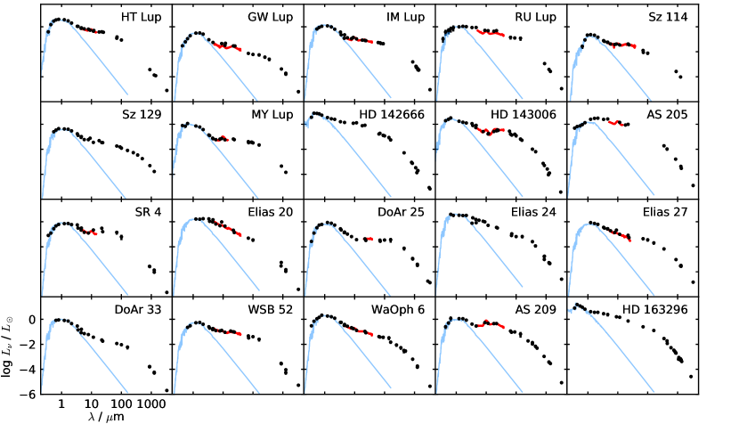
Figure 1: Broadband SEDs for the DSHARP targets. The ordinate is $L_{\nu}=4\pi d^{2}\nu F_{\nu}$ in $L_{\odot}$ units. These SEDs have been de-reddened using the extinction values quoted by the references in Col. (11) of Table 2 (second entries) and the prescription described by Andrews et al. (2013). Blue curves show the Nextgen/BT-settl photosphere models (Allard et al., 2003, 2011) corresponding to the stellar parameters listed in Table 2. Red curves show the Spitzer IRS spectra. Note that the SEDs for HT Lup and AS 205 include contributions from multiple components. Optical photometry was collected from a range of sources (Vrba et al., 1993; Herbst et al., 1994; Hughes et al., 1994; Oudmaijer et al., 2001; Wilking et al., 2005; Gras-Velázquez & Ray, 2005; Eisner et al., 2005; Padgett et al., 2006; Grankin et al., 2007; Merín et al., 2008; Mendigutía et al., 2012); infrared data were culled from 2MASS (Skrutskie et al., 2006), WISE (Wright et al., 2010), Spitzer imaging surveys (Carpenter et al., 2008; Evans et al., 2009), AKARI (Ishihara et al., 2010), and Herschel (IRSA); (sub-)mm data come from various sources (Andre & Montmerle, 1994; Mannings & Emerson, 1994; Sylvester et al., 1996; Nuernberger et al., 1997; Mannings & Sargent, 1997; Dent et al., 1998; Henning et al., 1998; Natta et al., 2004; Stanke et al., 2006; Andrews & Williams, 2007; Lommen et al., 2007, 2009; Roccatagliata et al., 2009; Andrews et al., 2009; Isella et al., 2007; Pinte et al., 2008; Isella et al., 2009; Ricci et al., 2010; Sandell et al., 2011; Öberg et al., 2011; Pérez et al., 2012, 2015; Qi et al., 2015; Ansdell et al., 2016; Cleeves et al., 2016; Barenfeld et al., 2016; Ubach et al., 2017; Huang et al., 2017; Tripathi et al., 2017; Cox et al., 2017; Andrews et al., 2018). These SEDs are available in the DSHARP data release.

The resulting sample and its stellar host properties are compiled in Table 2. Target distances ($d$) were derived from Gaia DR2 parallax measurements (Gaia Collaboration et al., 2018), following Astraatmadja & Bailer-Jones (2016) for a flat $d$ prior. Literature estimates of the effective temperatures ($T_{\rm eff}$) and luminosities ($L_{\ast}$; re-scaled for the appropriate $d$) were adopted to derive masses ($M_{\ast}$) and ages ($t_{\ast}$) based on the MIST models (Choi et al., 2016), following the methodology described by Andrews et al. (2018). Accretion rates ($\dot{M}_{\ast}$) were calculated from those host parameters and literature measurements of accretion luminosities (scaled for $d$; see Table 2). The sample hosts exhibit a range of young star properties, with $M_{\ast}\approx 0.2$–2 $M_{\odot}$ and nearly two decades spanned in both $L_{\ast}$ and $\dot{M}_{\ast}$. The mean age is 1 Myr, although with considerable individual uncertainties (and various untreated systematics; see Soderblom et al. 2014).

The broadband spectral energy distributions (SEDs) for the sample are shown together in Figure 1. Relative to the median SED (normalized at 1.5 $\mu$m) of larger samples of Class II targets (e.g., Ribas et al., 2017), RU Lup, AS 205, and AS 209 are in the top quartile (i.e., are over-luminous); the SEDs for HD 143006, SR 4, and DoAr 25 are relatively low in the near-infrared and high in the far-infrared (similar to, though not nearly as pronounced as, the typical transition disk SED); and the SEDs for DoAr 33 and WaOph 6 are in the bottom quartile. This diversity in the SEDs is one potential basis for future explorations of how the resolved emission distributions vary with relevant “bulk” parameters (e.g., the amount of dust settling toward the disk midplane).

While these sample targets do cover a range of properties, it is worth emphasizing that this range is not representative of the general population. The sample hosts tend to have earlier spectral types, and are accordingly more massive, luminous, and accreting more vigorously than stars at the peak of the initial mass function. This host bias enters implicitly with the sensitivity criterion, since we required a previous resolved measurement. The studies that provided those data are biased toward brighter continuum sources, which permeates to the host properties since the continuum luminosity scales steeply with $M_{\ast}$ (Andrews et al., 2013; Mohanty et al., 2013) and $\dot{M}_{\ast}$ (Manara et al., 2016; Mulders et al., 2017). The same is true for multiple star systems: these were not explicitly excluded, but the selection criteria bias against them because close companions tend to reduce the system continuum emission (e.g., Jensen et al., 1994; Harris et al., 2012).

The bias in favor of targets with brighter continuum emission also translates into a preferential selection of larger disks, given the observed size-luminosity correlation (Tripathi et al., 2017; Tazzari et al., 2017; Andrews et al., 2018). This corresponding size bias is decidedly beneficial for achieving the DSHARP goals discussed in Section 1. As we noted above, the general theoretical predictions for substructure sizes are comparable to the gas pressure scale height ($h_{P}$), which increases roughly linearly with disk radius. For a fixed resolution, it should be easier to identify and characterize the larger substructures expected at larger disk radii.

To roughly quantify these biases, we can make a comparison between targets that are more representative of the general disk population and the average member of the DSHARP sample. A “typical” target has a host star mass near the peak of the mass function ($M_{\ast}\approx 0.3$ $M_{\odot}$, or spectral type M3–M4) and continuum emission from its disk that is both relatively faint ($F_{\nu}\approx 10$–15 mJy; Ansdell et al. 2016; Cieza et al. 2019) and compact ($R_{\rm eff}\approx 10$–20 au, with the effective radius defined by Tripathi et al. 2017; see also Andrews et al. 2018). The DSHARP averages are $M_{\ast}\approx 0.8$ $M_{\odot}$ (spectral type K7), $F_{\nu}\approx 150$ mJy, and $R_{\rm eff}\approx 50$ au; only the sample extremes stretch down toward “typical” values.

These biases are difficult to mitigate for studies focused on finding and characterizing disk substructures, presuming their size scales are usually comparable to $h_{P}$. The “typical” disk is compact enough that $h_{P}$ for the radii where there is still continuum emission is smaller than the best resolutions available with ALMA. If this is the case, then we could be left probing only the extreme large end of substructures in “typical” disks, making any assessments of prevalence difficult (i.e., failed searches for substructures would still permit plenty of $h_{P}$-sized features to be present on sub-resolution scales). One option is to push to higher frequencies and thereby better resolution, but then high optical depths would limit the discovery-space to substructures in the form of dramatic depletions (e.g., very deep gaps) only.

Table 2: DSHARP Observing Log (ALMA Program 2016.1.00484.L)

Name	UTC Date	Config.	Baselines	$N_{\rm ant}$	$\mathcal{E}/\arcdeg$	PWV/mm	Calibrators
HT Lup	2017/05/14–04:11	C40-5	015 m – 01.1 km	43	76–77	1.00–1.15	J1517-2422, J1427-4206, J1610-3958, J1540-3906
	2017/05/17–02:12	C40-5	015 m – 01.1 km	49	58–67	0.90–1.05	J1517-2422, J1517-2422, J1610-3958, J1540-3906
	2017/09/24–17:39	C40-8/9	041 m – 12.1 km	39	59–70	0.60–1.15	J1517-2422, J1517-2422, J1534-3526, J1536-3151
	2017/09/24–19:12	C40-8/9	041 m – 12.1 km	39	75–78	0.65–1.05	J1517-2422, J1427-4206, J1534-3526, J1536-3151
GW Lup	2017/05/14–04:11	C40-5	015 m – 01.1 km	43	69–72	1.00–1.15	J1517-2422, J1427-4206, J1610-3958, J1540-3906

Note. — Col. (1) Target name. Col. (2) UTC date and time at the start of the observations. Col. (3) ALMA configuration. Col. (4) Minimum and maximum baseline lengths. Col. (5) Number of antennas available. Col. (6) Target elevation range. Col. (7) Range of precipitable water vapor levels. Col. (8) From left to right, the quasars observed for calibrating the bandpass, amplitude scale, phase variations, and checking the phase transfer. Additional archival observations used in our analysis are compiled in Table 2. Table 2 is published in its entirety in the electronic edition of the journal. A portion is shown here for guidance regarding its form and content.

Table 3: Archival ALMA Datasets Used by DSHARP

Name	UTC Date	Config.	Baselines	$N_{\rm ant}$	Calibrators	Program	References
IM Lup	2014/07/06–22:18	C34-4	20 – 0650 m	31	J1427-4206, Titan, J1534-3526, J1626-2951	2013.1.00226.S	1
	2014/07/17–01:38	C34-4	20 – 0650 m	32	J1427-4206, Titan, J1534-3526,  $\cdots$ 0000	2013.1.00226.S	1
	2015/01/29–09:48	C34-2/1	15 – 0349 m	40	J1517-2422, Titan, J1610-3958,  $\cdots$ 0000	2013.1.00694.S	2
	2015/05/13–08:30	C34-3/4	21 – 0558 m	36	J1517-2422, Titan, J1610-3958,  $\cdots$ 0000	2013.1.00694.S	2
	2015/06/09–23:42	C34-5	21 – 0784 m	37	J1517-2422, Titan, J1610-3958, J1614-3543	2013.1.00798.S	3

Note. — Col. (1) Target name. Col. (2) UTC date and time at the start of the observations. Col. (3) ALMA configuration. Col. (4) Range of baseline lengths. Col. (5) Number of antennas available. Col. (6) From left to right, the quasars observed for calibrating the bandpass, amplitude scale, phase variations, and checking the phase transfer. An entry of ‘$\ldots$’ indicates no calibrator was observed for checking the phase transfer. Col. (7) ALMA program ID. Col. (8) Original references for these datasets. Table 2 is published in its entirety in the electronic edition of the journal. A portion is shown here for guidance regarding its form and content.

References. — 1 = Öberg et al. (2015), 2 = Cleeves et al. (2017), 3 = Pinte et al. (2018), 4 = Salyk et al. (2014), 5 = Dipierro et al. (2018), 6 = Pérez et al. (2016), 7 = Huang et al. (2016), 8 = Fedele et al. (2018), 9 = Flaherty et al. (2015), 10 = Isella et al. (2016).

3 Observations

The DSHARP ALMA observations were conducted in 2017 May–November as part of program 2016.1.00484.L. All measurements used the Band 6 receivers and correlated data from four spectral windows (SPWs) in dual polarization mode. The continuum was sampled in three SPWs, centered at 232.6, 245.0, and 246.9 GHz, each with 128 channels spanning 1.875 GHz (31.25 MHz per channel). The remaining SPW was centered at the ¹²CO $J$=2$-$1 rest frequency (230.538 GHz) and covered a bandwidth of 938 MHz in 3840 channels (488 kHz channel spacing, 0.64 km s^-1 velocity resolution). The plan was to observe each target briefly in the C40-5 (hereafter “compact”) configuration, and also for $\sim$1 hour in the C40-8 or C40-9 (hereafter “extended”) configurations. The compact observations are necessary to recover emission on the larger angular scales that are not sampled in the extended configurations. The actual observing log is provided in Table 2.

The compact observations used an array with baseline lengths from 15 m to 1.1 km (a resolution of $\sim$0$\farcs$25). The FWHM continuum and CO (per channel) emission scales are $\lesssim$ 2″, so spatial filtering should be negligible (cf., Wilner & Welch, 1994). These observations cycled between nearby targets and totaled $\sim$12 minutes of integration time per source. A nearby phase calibrator was observed every 6 minutes; an additional “check” calibrator (to assess the quality of phase transfer) was observed every 30 minutes. A bandpass and amplitude calibrator (sometimes the same quasar) were observed during each observing block. The log in Table 2 includes information about the observing conditions and calibrators.

We relied on archival ALMA observations of 5 targets (IM Lup, HD 142666, Elias 24, Elias 27, HD 163296) instead of obtaining new compact data, and folded in archival data for 3 other targets (HD 143006, AS 205, AS 209). Information about these datasets are compiled in Table 2. The setups, observing strategies, and weather conditions are described in the listed references.

Due to a long stretch of inclement weather, the extended configuration observations were delayed until 2017 September, and continued through November. Despite the non-optimal scheduling for the DSHARP sample, nearly all of the targets were observed for two executions (often in different configurations) in good conditions, each with $\sim$35 minutes of on-source integration time. Sz 114, AS 205, and DoAr 25 each had only a single successful execution. The spectral setup was the same as for the compact datasets. Observations cycled between a single target and a nearby phase calibrator on 1 minute intervals, with a “check” calibrator visited every 30 minutes. Bandpass and amplitude calibrators were observed in each execution block (see Table 2).

4 Calibration and Imaging

Since the DSHARP survey is among the first to collect a large volume of ALMA data on such long baselines, a substantial effort was made to explore various calibration strategies to enhance the data quality. The standard methodology we adopted is described here. The specific details on the calibration of datasets for individual targets (i.e., calibration scripts) are available in the DSHARP data release (see Section 5). All calibration tasks are performed with the CASA package (McMullin et al., 2007) and a small supplement of python tasks.

4.1 Pipeline Calibration

The first step was a standard ALMA pipeline calibration. This procedure was performed by ALMA staff separately for the compact and extended data, using CASA v4.7.2 or v5.1.1 for datasets that were processed before or after 2017 November, respectively. The pipeline imports the raw data and flags problematic scans, channels, or antennas. It then derives a table of system temperatures ($T_{\rm sys}$). Most of the DSHARP data have $T_{\rm sys}\approx 60$–80 K; in the poorest conditions it reached 130 K, and in the best cases it was 50 K. Next, the pipeline adjusts the visibility phases according to water vapor radiometer (WVR) measurements. For the extended data, the WVR corrections improved the median RMS phase variations by a factor of $\sim$1.7, although individual datasets saw improvements between 1.2–3. The corrected RMS phase variations (far from the reference antenna) were typically 30° (with a range $\sim$15–50°). The compact observations saw similar improvement factors (1.5–3.0) and RMS phase variations ($\sim$10°).

The pipeline then performs a bandpass calibration, using the first quasar in the calibrator list in Table 2. It continues by setting the amplitude scale, using measurements of the second quasar in the Table 2 list. The flux density in each SPW for that quasar is determined from a power-law spectral model based on bi-monthly monitoring in ALMA Bands 3 and 7 ($\sim$100 and 340 GHz) that is tied to primary calibrators (planets or moons). Finally, the gain variations with time are corrected, with reference to repeated measurements of the nearby quasar listed third in the Table 2 calibrator list.

4.2 Self-Calibration

We next performed some substantial post-processing, with particular emphasis on combining datasets (from different array configurations and observations) and self-calibrating the visibilities. We generally followed the homogenized strategy described below, using CASA v5.1.1 and a set of custom python routines.

The procedure started with the compact data. A pseudo-continuum dataset was created by flagging data within $\pm$25 km s^-1 from the CO $J$=2$-$1 line center and averaging into 125 MHz channels. The visibilities corresponding to each individual observation were imaged (Section 4.3) and checked to ensure consistent astrometric registration and flux calibration (if necessary, they are corrected; see Section 4.4). The individual datasets were then re-combined. Next, we performed a series of phase-only self-calibration iterations, stepping down the solution interval (60, 30, 18, and 6 s). Reference antennas were selected based on data quality and proximity to the array center. When possible, we avoided combining SPWs (or scans) to correct for SPW-dependent gain variations. After each iteration, the data were imaged. A noise estimate was made in an annular region within a 4$\farcs$25-radius circle centered on the target but excluding the image mask. This self-calibration sequence is stopped after reaching a solution interval on the record length (6 s) or if the peak SNR does not increase by $>5$% from the previous iteration. Finally, we performed one iteration of amplitude self-calibration (for each SPW independently) on a scan interval ($\sim$6 minutes). The (phase + amplitude) self-calibration provided a dramatic improvement in quality. The typical peak SNR increased by a factor of 3; the resulting noise was 30 $\mu$Jy beam^-1 (10 mK) for a $\sim$0$\farcs$25 beam. The same procedure was applied to archival datasets.

Next, we prepared the extended data as was described above, with an additional time-averaging to 6 s integrations (from the original 2 s records). The data for each individual extended observation were imaged and checked for misalignments and flux discrepancies. Once those are corrected (if necessary; see Section 4.4), the compact (already self-calibrated) and extended datasets were combined. The phases for this combined dataset were iteratively self-calibrated on solution intervals of {900, 360, 180, 60, 30 s} (usually only the latter 3 are necessary). The SPWs were combined in this case to enhance the SNR on longer baselines. For antenna pairings with SNR $\leq 1.5$ on these intervals, the self-calibration solutions were not applied but the corresponding data were not flagged (applymode=‘calonly’ in the applycal task). The sequence was stopped when the peak SNR does not increase by $>5$% and the map quality does not visually improve. One iteration of amplitude self-calibration was attempted on the starting interval of the phase self-calibration sequence.

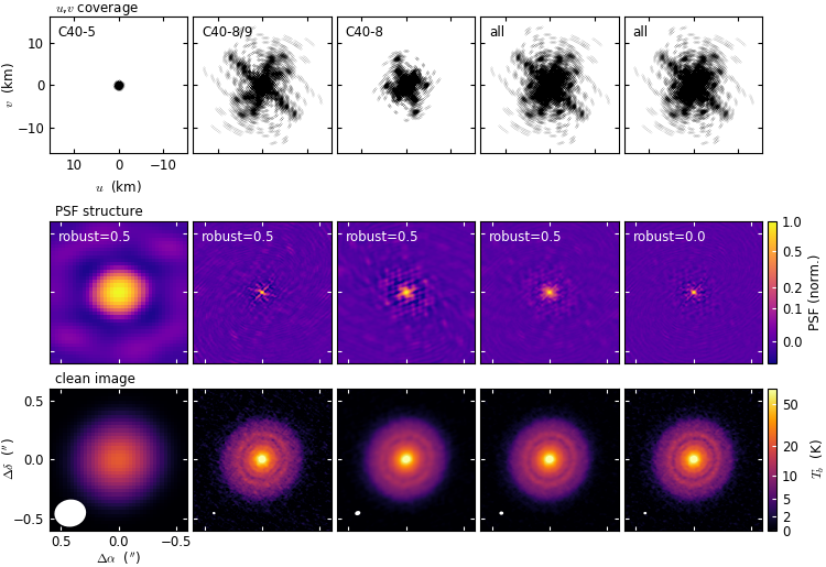
Figure 2: Illustration of the effects of spatial frequency coverage and visibility weighting on PSF structure and image morphology, for the RU Lup disk. The top panels show the observed $u$,$v$ coverage. The middle panels show the corresponding PSF structures, annotated with the corresponding robust weighting parameter. The bottom panels show the corresponding images, on the same $T_{b}$ scale, created from subsets of the end product of the self-calibration. FWHM beam dimensions are marked in the lower left corners of each image.

This self-calibration of the combined datasets resulted in a typical improvement of 40% in the peak SNR, although there is a large range in benefits across the sample. The improvements are generally smaller here because the compact data were already self-calibrated and the extended data were taken in excellent conditions. The typical noise measured in the combined, self-calibrated datasets is 10–20 $\mu$Jy beam^-1 (0.1–0.5 K).

Once the continuum self-calibration was satisfactory, the same gain tables are applied to the non-spectrally-averaged visibilities (after any required astrometric and flux calibration adjustments) to obtain a corresponding calibrated measurement set for the region of the spectrum around the CO $J$=2$-$1 emission line.

4.3 Imaging During Self-Calibration

Self-calibration uses continuum emission models assembled from the ‘clean’ components derived from interferometric imaging. We adopted a set of imaging standards to homogenize that process. These were informed by considerable experimentation with the associated parameter choices. We explored alternative sets of deconvolution scales, clean thresholds, masks, and pixel sizes and found that reasonable other options had negligible influence on the end products of self-calibration.

All imaging was performed with the tclean task. For the compact data, we imaged out to the primary beam FWHM (26″) with 30 mas pixels ($\sim$10 per synthesized beam FWHM, $\theta_{b}$) to check for problematic background sources. Finding nothing of concern, we used 9″-wide images with 3 mas pixels (again, $\sim$10 pixels per $\theta_{b}$) for the combined datasets. We used the multi-scale, multi-frequency synthesis (assuming a flat spectrum) deconvolution mode (Cornwell, 2008) with a Briggs robust=0.5 weighting scheme. Elliptical masks were designed to reflect the target geometry (aspect ratio, position angle) and pad the outer reaches of the emission distribution. The adopted (Gaussian) deconvolution scales are target-dependent, but always include a point-like contribution and scales comparable to $\theta_{b}$ and 2–$3\times\theta_{b}$; additional scales (increasing by factors of 2–3) could be selected up to the mask radius. The algorithm was halted on thresholds; 3$\times$ the noise early in the self-calibration sequence, and 2$\times$ the noise for the last phase-only step and the amplitude self-calibration.

Table 4: DSHARP Fiducial Continuum Image Properties

Name	$\nu$	$\theta_{b}$, 00PAb	RMS noise	peak $I_{\nu}$, $T_{b}$	$F_{\nu}$	robust	$\theta_{\rm tap}$, .PAtap	Refs.
	(GHz)	(mas, 00°)	($\mu$Jy beam-1, K)	(mJy beam-1, K)	(mJy)		(mas, 00°)
HT Lup	239.0	$38\times 33$, 061	14, 000.24	8.25, 0140	077	0.0.5	$\cdots$	IV
GW Lup	239.0	$45\times 43$, 001	15, 000.17	3.35, 0037	089	0.0.5	$35\times 15$, 000	II
IM Lup	239.0	$44\times 43$, 115	14, 000.16	7.11, 0080	253	0.0.5	$33\times 26$, 138	II, III
RU Lup	239.0	$25\times 24$, 129	21, 000.73	3.45, 0123	203	$-$0.5	$22\times 10$, 174	II
Sz 114	239.0	$67\times 28$, 092	19, 000.22	3.36, 0038	049	0.0.5	$\cdots$	II
Sz 129	239.0	$44\times 31$, 094	15, 000.24	0.96, 0015	086	0.0.0	$\cdots$	II
MY Lup	239.0	$44\times 43$, 122	16, 000.18	1.78, 0020	079	0.0.0	$39\times 15$, 163	II
HD 142666	231.9	$32\times 22$, 062	13, 000.35	1.28, 0041	130	0.0.5	$\cdots$	II
HD 143006	239.0	$46\times 45$, 051	15, 000.15	0.67, 0007	059	0.0.0	$42\times 20$, 172	II, X
AS 205	233.7	$38\times 25$, 095	16, 000.38	6.15, 0145	358	0.0.5	$\cdots$	IV
SR 4	239.0	$34\times 34$, 010	25, 000.46	3.40, 0063	069	$-$0.5	$35\times 10$, 000	II
Elias 20	239.0	$32\times 23$, 076	15, 000.44	2.59, 0075	104	0.0.0	$\cdots$	II
DoAr 25	239.0	$41\times 22$, 070	13, 000.31	1.35, 0032	246	0.0.5	$\cdots$	II
Elias 24	231.9	$37\times 34$, 082	19, 000.49	4.63, 0119	352	0.0.0	$35\times 10$, 166	II
Elias 27	231.9	$49\times 47$, 047	14, 000.14	4.83, 0048	330	0.0.5	$40\times 20$, 173	II, III
DoAr 33	239.0	$37\times 24$, 075	17, 000.41	1.89, 0046	035	0.0.0	$20\times 10$, 167	II
WSB 52	239.0	$33\times 27$, 074	16, 000.38	2.60, 0062	067	0.0.0	$\cdots$	II, III
WaOph 6	239.0	$58\times 54$, 084	17, 000.12	8.67, 0059	161	0.0.0	$55\times 10$, 010	II, III
AS 209	239.0	$38\times 36$, 068	19, 000.30	1.83, 0029	288	$-$0.5	$37\times 10$, 162	II, VIII
HD 163296	239.0	$48\times 38$, 082	23, 000.27	4.26, 0050	715	$-$0.5	$\cdots$	II, IX

Note. — Col. (1) Target name. Col. (2) Mean frequency. Col. (3) Synthesized beam FWHM and position angle. Col. (4) RMS noise in the map, as described in Section 4.3. Col. (5) Peak intensity in the map. Note that noise and peak brightness temperatures are calculated assuming the Rayleigh-Jeans limit. Col. (6) Integrated flux density inside the image mask. Col. (7) Briggs robust value. Col. (8) FWHM and position angle of the taper (if applicable).

References. — II = Huang et al. (2018a), III = Huang et al. (2018b), IV = Kurtovic et al. (2018), VIII = Guzmán et al. (2018), IX = Isella et al. (2018), X = Pérez et al. (2018).

Special effort was made to verify that sidelobes in the point spread function (PSF, or ‘dirty’ beam) do not corrupt the self-calibration. The extended ALMA configurations place antennas along three distinct arms (set by the site topography). The corresponding spatial frequency coverage generates complicated PSF features, with sidelobes up to $\sim$30%. Figure 2 illustrates the impact, showing the connections between the sampling function ($u$,$v$ coverage), PSF, and image for different configurations and weighting schemes. We vetted the effects of those PSF features on self-calibration by repeating the process for different combinations of weighting schemes and tapers. Coupling lower robust values with tapers can mitigate PSF artifacts while maintaining resolution, but at a substantial SNR cost. Direct comparisons (of both visibilities and images) between these variants and the standard methodology outlined above demonstrated that the PSF features had negligible impact on the self-calibration.

While the effects on self-calibration are minimal, the resulting images can still exhibit PSF-related artifacts. One of the more interesting is the imprint of a hexagonal structure on emission rings (e.g., second image from left, bottom row of Figure 2), produced by convolution with a “spoked” PSF (a consequence of the the extended ALMA configuration arms). As demonstrated in the bottom right panel, this can usually be minimized with an appropriate visibility weighting and/or tapering.

4.4 Astrometric and Flux Scale Alignment

Half the sample targets show clear spatial offsets between their emission centers in different observations. For the larger of these shifts ($\sim$100 mas), the cause is proper motion (especially when using archival data); in other cases, smaller (10–30 mas) mismatches might instead be attributed to instrumental or atmospheric artifacts. Combining these datasets without correcting these shifts creates blurred (or even double) images, which is problematic when they are used as initial self-calibration models. The solution is to simply adjust the visibility phases to shift into alignment. We measure emission centroid positions with Gaussian fits in the image plane for each individual observation and calculate the offsets relative to the highest quality extended dataset. The fixvis task then implements the appropriate phase adjustments. In cases where the observations have different pointing centers, we manually reconcile them with the fixplanets task.

We also routinely found mismatches in the amplitude scales among different observations of a target. Some experimentation showed that noticeably improved self-calibration results were obtained if the relative flux scales between observations were consistent within 5%. To quantify any mismatches, we inspected the deprojected (according to the Gaussian fit geometries noted above), azimuthally-averaged visibilities from different datasets on 200-500 k$\lambda$ baseline lengths (at lower spatial frequencies, the extended configuration data are too sparse, and at higher frequencies the averages are more strongly affected by low SNR and phase noise).

These mismatches are caused by inaccurate flux calibration. The claimed calibration accuracy is $\sim$10%, although the adopted methodology for estimating calibrator fluxes (interpolation in time and frequency) can lead to some added uncertainty. About a third of the sample had 5–10% mismatches, but the majority exhibited 15–25% discrepancies for at least one dataset. In some cases, these were tracked down to a bookkeeping issue: the data were pipeline-processed before a relevant calibrator catalog update. Some 2017 November datasets that used J1427-4206 as the calibrator were problematic. There is no obvious error in the calibrator catalog, so the issue must be with the interpolation: perhaps this quasar flared or changed its spectrum between catalog entries. Regardless of the cause, these misalignments were rectified. We selected a reference dataset and used the gaincal task to re-scale the outlier datasets.

4.5 Fiducial Images

After the calibration was complete, we synthesized a set of fiducial images for further analysis. The continuum imaging followed the methodology outlined in Section 4.3, but was tailored to individual sources with the aim of minimizing PSF artifacts. In many cases, this involved adopting a visibility weighting scheme that traded SNR for resolution, as well as a visibility taper to improve the PSF symmetry. Table 4.3 lists the basic parameters and resulting properties of these fiducial images. A gallery of the continuum images are shown in Figure 3. Small-scale substructures are notable in all of the DSHARP targets, often with compact (FWHM $\lesssim$ 10 au) dimensions. Figure 4 emphasizes the utility of pushing the ALMA resolution for recovering such features in one particularly illustrative example.

We also synthesized channel maps of the CO $J$=2$-$1 emission following the basic steps outlined above. The self-calibrated CO visibilities were continuum-subtracted and imaged in LSRK velocity channels at roughly the native channel spacing (0.35 km s^-1; the actual velocity resolution is about two channels, due to Hanning smoothing in the ALMA correlator). The DSHARP data are generally not sensitive enough to reconstruct useful channel maps of the emission line at the best available resolution. We compromised by increasing the relative weight of shorter baselines and employing a modest taper. Table 5 lists the imaging parameters, and Figure 5 shows the channel maps. For many of the targets, the CO channel maps exhibit partially recovered large-scale emission structures from the ambient cloud material. These are noted in Table 5 to prevent confusion in the interpretation of extended emission features in some cases (e.g., Elias 24 and WSB 52 are particularly problematic cases).

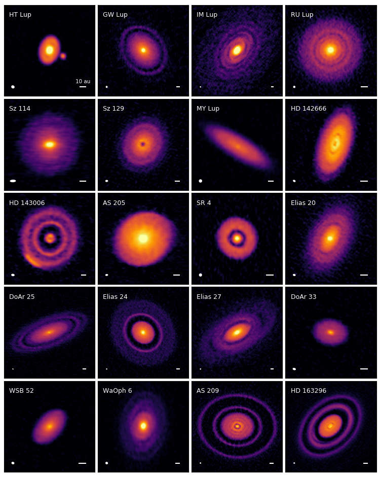
Figure 3: A gallery of 240 GHz (1.25 mm) continuum emission images for the disks in the DSHARP sample. Beam sizes and 10 au scalebars are shown in the lower left and right corners of each panel, respectively. All images are shown with an asinh stretch to reduce the dynamic range (accentuate fainter details without over-saturating the bright emission peaks). For more quantitative details regarding the image dimensions and intensity scales, see Huang et al. (2018a) and Kurtovic et al. (2018).

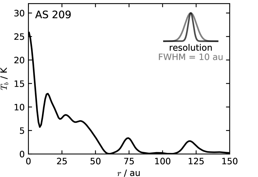
Figure 4: The deprojected, azimuthally-averaged radial brightness temperature profile for the 240 GHz continuum emission from the AS 209 disk (see Huang et al., 2018a; Guzmán et al., 2018, for more details). The corresponding image is shown in the bottom row of Figure 3, second from right. The PSF profile (resolution) is marked in black in the upper right corner, along with a gray Gaussian profile that has FWHM = 10 au, to illustrate that the disk substructures typically have compact dimensions.

5 Data Release

One key inspiration for conducting the DSHARP survey was to provide a set of resources to the community that can seed and develop a range of related work. To that end, we have released a suite of data products that go beyond the standard contents in the ALMA archive. This release is available online at https://almascience.org/alma-data/lp/DSHARP. It includes: (1) CASA scripts and associated python modules used to calibrate and image the data; (2) fully calibrated continuum and CO measurement sets (visibility datafiles); (3) continuum images and CO channel maps; and (4) some secondary products (radial intensity profiles, SED data). With this data release and the standard ALMA archive products, the community has the access needed to both reproduce and expand on the efforts detailed in the initial series of DSHARP articles.

Table 5: DSHARP Fiducial CO Datacube Properties

Name	$\theta_{b}$, 00PAb	RMS noise	peak $I_{\nu}$, $T_{b}$	robust	$\theta_{\rm tap}$, .PAtap	comments	Refs.
	(mas, 00°)	(mJy beam-1, K)	(mJy beam-1, K)		(mas, 00°)
HT Lup	$\phantom{0}53\times\phantom{0}50$, 0066	1.2, 010.1	12.8, 0111	0.5	$\cdots$	cloud (severe); $<150$ m filter	IV
GW Lup	$109\times\phantom{0}81$, 0097	1.4, 003.5	20.9, 0054	1.0	$\phantom{0}40\times\phantom{0}40$,  $\cdots$	$\cdots$	$\cdots$
IM Lup	$122\times 115$, 0047	1.9, 003.2	34.4, 0056	0.0	$100\times 100$,  $\cdots$	$\cdots$	III
RU Lup	$\phantom{0}95\times\phantom{0}83$, 0072	1.2, 003.4	49.7, 0146	1.0	$\phantom{0}40\times\phantom{0}40$,  $\cdots$	cloud (mild), complex outflow	$\cdots$
Sz 114	$130\times\phantom{0}90$, 0105	2.0, 004.0	26.8, 0053	1.0	$\phantom{0}40\times\phantom{0}40$,  $\cdots$	cloud (moderate)	$\cdots$
Sz 129	$110\times\phantom{0}83$, 0076	1.0, 002.6	15.3, 0038	1.0	$\phantom{0}40\times\phantom{0}40$,  $\cdots$	$\cdots$	$\cdots$
MY Lup	$100\times\phantom{0}82$, 0079	1.1, 003.1	15.4, 0043	1.0	$\phantom{0}40\times\phantom{0}40$,  $\cdots$	cloud (mild)	$\cdots$
HD 142666	$\phantom{0}77\times\phantom{0}61$, 0081	1.3, 006.3	12.4, 0061	1.0	$\phantom{0}40\times\phantom{0}40$,  $\cdots$	$\cdots$	$\cdots$
HD 143006	$\phantom{0}66\times\phantom{0}49$, 0084	1.0, 007.1	11.2, 0080	0.8	$\phantom{0}20\times\phantom{0}20$,  $\cdots$	$\cdots$	X
AS 205	$115\times\phantom{0}92$, 0093	1.4, 003.2	75.9, 0166	1.0	$\phantom{0}40\times\phantom{0}40$,  $\cdots$	$\cdots$	IV
SR4	$111\times\phantom{0}87$, 0090	1.5, 003.5	29.9, 0071	1.0	$\phantom{0}40\times\phantom{0}40$,  $\cdots$	cloud (moderate)	$\cdots$
Elias 20	$102\times\phantom{0}72$, 0088	1.8, 005.6	27.0, 0085	1.0	$\phantom{0}40\times\phantom{0}40$,  $\cdots$	cloud (severe), outflow	$\cdots$
DoAr 25	$101\times\phantom{0}78$, 0087	1.3, 003.9	18.9, 0055	1.0	$\phantom{0}40\times\phantom{0}40$,  $\cdots$	cloud (moderate)	$\cdots$
Elias 24	$\phantom{0}94\times\phantom{0}60$, 0090	1.5, 006.2	23.6, 0097	1.0	$\phantom{0}40\times\phantom{0}40$,  $\cdots$	cloud (severe)	$\cdots$
Elias 27	$132\times 111$, 0123	1.6, 002.5	44.9, 0071	1.0	$100\times\phantom{0}70$, 0145	cloud (moderate), envelope$?$	III
DoAr 33	$103\times\phantom{0}79$, 0088	1.3, 003.6	15.8, 0045	1.0	$\phantom{0}40\times\phantom{0}40$,  $\cdots$	cloud (mild)	$\cdots$
WSB 52	$114\times\phantom{0}80$, 0090	1.1, 002.8	31.4, 0079	1.0	$\phantom{0}40\times\phantom{0}40$,  $\cdots$	cloud (severe), complex outflow	$\cdots$
WaOph 6	$126\times 115$, 0100	1.3, 002.1	41.0, 0065	0.5	$100\times\phantom{0}30$, 0017	cloud (mild)	III
AS 209	$\phantom{0}95\times\phantom{0}72$, 0096	0.9, 002.9	21.4, 0072	1.0	$\phantom{0}25\times\phantom{0}10$, 0010	cloud (mild)	VIII
HD 163296	$104\times\phantom{0}95$, 0100	0.8, 001.9	40.7, 0095	0.5	$\cdots$	$\cdots$	IX

Note. — Col. (1) Target name. Col. (2) Synthesized beam FWHM and position angle. Col. (3) RMS noise per channel, measured as described in Section 4.3. HD 143006 and HD 163296 are imaged with 0.32 km s^-1 channels; for all other targets, we used 0.35 km s^-1 channels. Col. (4) Peak intensity. Note that noise and peak brightness temperatures are calculated assuming the Rayleigh-Jeans limit. Col. (5) Briggs robust value. Col. (6) FWHM and position angle of the adopted taper (if applicable). Col. (7) Comments on issues with the channel maps, including degree of contamination from the ambient molecular cloud and the presence of non-disk features.

References. — III Huang et al. (2018b). IV Kurtovic et al. (2018). VIII Guzmán et al. (2018). IX Isella et al. (2018). X Pérez et al. (2018).

6 Overview: Initial DSHARP Results

This article has detailed the scientific motivations behind DSHARP, introduced the survey strategy and sample, described the observations and calibration process, and presented the resulting products as part of our data release. It is also the first in a series of articles that explore and analyze the data in more detail. The principal DSHARP conclusions can be summarized as follows:

$\bullet$ Continuum substructures are ubiquitous in this sample, as can be deduced from Figure 3. Small-scale emission features are found at effectively any disk radius, from 5 au out to more than 150 au.

$\bullet$ The most common form of these substructures are concentric bright rings and dark gaps. There are no obvious patterns in their distributions or connections to the stellar host properties. There are hints of ring/gap substructures that are obfuscated due to their smaller size scales (relative to the DSHARP resolution) and/or their modest amplitudes with respect to an optically thick background in the inner disk. Measurements of the rings and gaps, as well as a more detailed exploration of their potential origins and associated issues, are presented by Huang et al. (2018a).

$\bullet$ While less common, the spiral morphologies identified for a subset of disks in the DSHARP sample are striking. For the cases with apparently single host stars (IM Lup, Elias 27, and WaOph 6), the spiral patterns are complex and appear to be superposed with rings and gaps. Their emission distributions and potential origins are characterized by Huang et al. (2018b).

$\bullet$ For the two known multiple star systems in the DSHARP sample, HT Lup and AS 205, the disks around the primary stars show clear two-armed spirals and complicated CO distributions that are indicative of strong dynamical interactions. The circumstellar material in these systems is studied by Kurtovic et al. (2018).

$\bullet$ Azimuthal asymmetries are rare in this sample. Substantial deviations from axisymmetry (or point symmetry for the spirals) are only identified in two cases. The disks around HD 143006 and HD 163296 show small, arc-shaped features in otherwise emission-depleted regions (i.e., beyond the continuum disk edge and in a gap, respectively). The properties and potential origins of these special cases are scrutinized by Pérez et al. (2018) and Isella et al. (2018), respectively.

$\bullet$ In some cases, the continuum emission can be decomposed into only small-scale substructures. The AS 209 disk is a particularly compelling example. Guzmán et al. (2018) quantify its substructures and highlight an important point: there are analogous features lurking in the gas (even as traced by optically thick ¹²CO), at radii well beyond the extent of the continuum emission.

$\bullet$ The ring substructure sizes and amplitudes suggest that these features can be understood as dust trapped in axisymmetric gas pressure bumps. Dullemond et al. (2018) demonstrate this conclusion and derive a lower limit on the strength of the turbulence in the disk. These and other related analyses are guided by a fiducial dust model developed by Birnstiel et al. (2018).

$\bullet$ A new suite of hydrodynamics simulations by Zhang et al. (2018) suggest that dynamical interactions between low-mass (sub-Jupiter) planets and their local disk material are plausible explanations of the observed ring/gap substructures. Assuming this is the case, those simulations are used to reconstruct the associated planet population in the mass – semimajor axis plane.

There is, of course, much more to learn from the DSHARP dataset. Our hope is that this preliminary foray not only provides useful results and motivation for many other studies, but also lays some technical groundwork for designing and calibrating future ALMA surveys of disks at very high angular resolution.

Fig. Set5. DSHARP CO $J$=2$-$1 Channel Maps

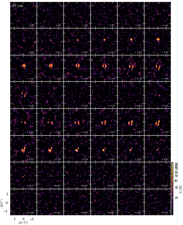
Figure 5.1: Channel maps of the ¹²CO $J$=2$-$1 line emission from the HT Lup disk.

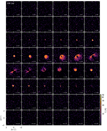
Figure 5.2: Channel maps of the ¹²CO $J$=2$-$1 line emission from the GW Lup disk.

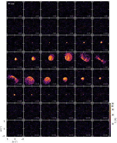
Figure 5.3: Channel maps of the ¹²CO $J$=2$-$1 line emission from the IM Lup disk.

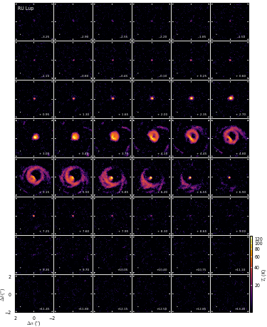
Figure 5.4: Channel maps of the ¹²CO $J$=2$-$1 line emission from the RU Lup disk.

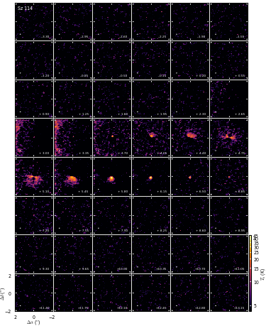
Figure 5.5: Channel maps of the ¹²CO $J$=2$-$1 line emission from the Sz 114 disk.

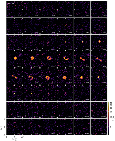
Figure 5.6: Channel maps of the ¹²CO $J$=2$-$1 line emission from the Sz 129 disk.

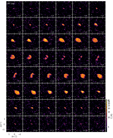
Figure 5.7: Channel maps of the ¹²CO $J$=2$-$1 line emission from the MY Lup disk.

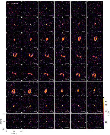
Figure 5.8: Channel maps of the ¹²CO $J$=2$-$1 line emission from the HD 142666 disk.

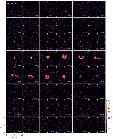
Figure 5.9: Channel maps of the ¹²CO $J$=2$-$1 line emission from the HD 143006 disk.

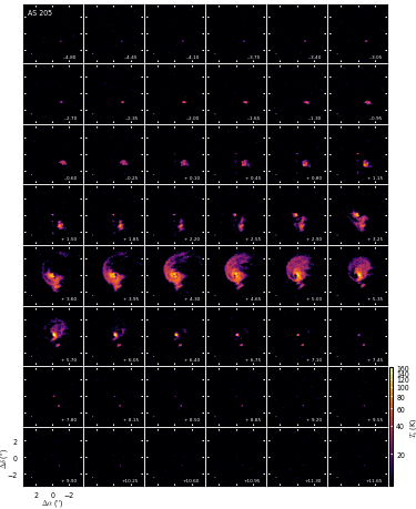
Figure 5.10: Channel maps of the ¹²CO $J$=2$-$1 line emission from the AS 205 disk.

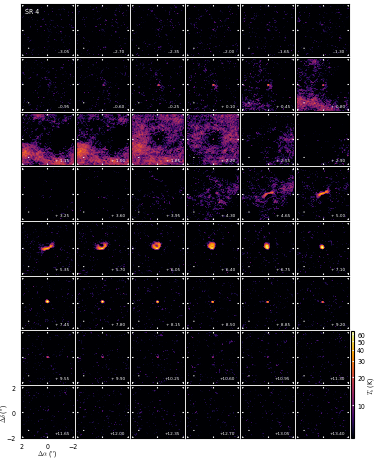
Figure 5.11: Channel maps of the ¹²CO $J$=2$-$1 line emission from the SR 4 disk.

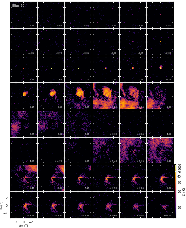
Figure 5.12: Channel maps of the ¹²CO $J$=2$-$1 line emission from the Elias 20 disk.

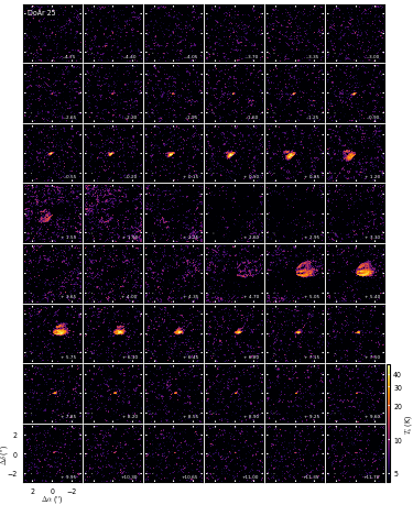
Figure 5.13: Channel maps of the ¹²CO $J$=2$-$1 line emission from the DoAr 25 disk.

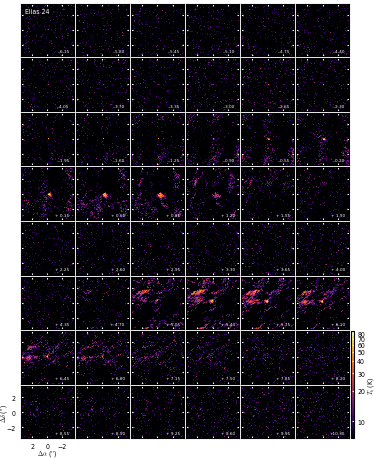
Figure 5.14: Channel maps of the ¹²CO $J$=2$-$1 line emission from the Elias 24 disk.

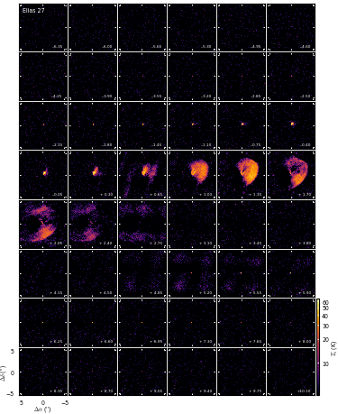
Figure 5.15: Channel maps of the ¹²CO $J$=2$-$1 line emission from the Elias 27 disk.

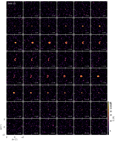
Figure 5.16: Channel maps of the ¹²CO $J$=2$-$1 line emission from the DoAr 33 disk.

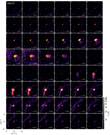
Figure 5.17: Channel maps of the ¹²CO $J$=2$-$1 line emission from the WSB 52 disk.

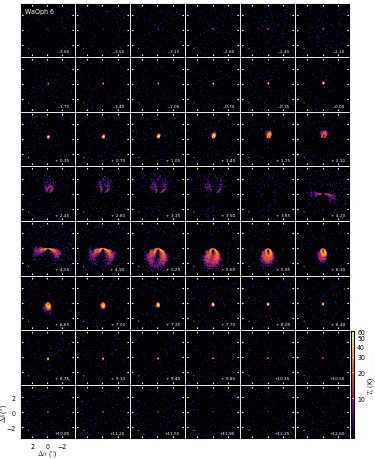
Figure 5.18: Channel maps of the ¹²CO $J$=2$-$1 line emission from the WaOph 6 disk.

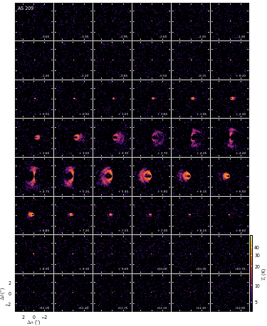
Figure 5.19: Channel maps of the ¹²CO $J$=2$-$1 line emission from the AS 209 disk.

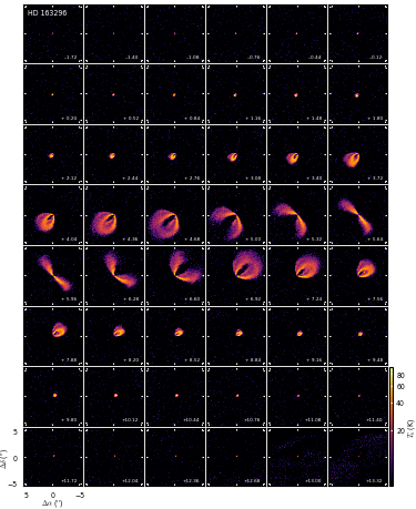
Figure 5.20: Channel maps of the ¹²CO $J$=2$-$1 line emission from the HD 163296 disk.

Table 2: DSHARP Observing Log (ALMA Program 2016.1.00484.L)

Name	UTC Date	Config.	Baselines	$N_{\rm ant}$	$\mathcal{E}/\arcdeg$	PWV/mm	Calibrators
HT Lup	2017/05/14–04:11	C40-5	015 m – 01.1 km	43	76–77	1.00–1.15	J1517-2422, J1427-4206, J1610-3958, J1540-3906
	2017/05/17–02:12	C40-5	015 m – 01.1 km	49	58–67	0.90–1.05	J1517-2422, J1517-2422, J1610-3958, J1540-3906
	2017/09/24–17:39	C40-8/9	041 m – 12.1 km	39	59–70	0.60–1.15	J1517-2422, J1517-2422, J1534-3526, J1536-3151
	2017/09/24–19:12	C40-8/9	041 m – 12.1 km	39	75–78	0.65–1.05	J1517-2422, J1427-4206, J1534-3526, J1536-3151
GW Lup	2017/05/14–04:11	C40-5	015 m – 01.1 km	43	69–72	1.00–1.15	J1517-2422, J1427-4206, J1610-3958, J1540-3906
	2017/05/17–02:12	C40-5	015 m – 01.1 km	49	51–61	0.90–1.05	J1517-2422, J1517-2422, J1610-3958, J1540-3906
	2017/09/24–23:31	C40-8/9	041 m – 14.9 km	40	29–39	0.80–1.20	J1617-5848, J1733-1304, J1534-3526, J1536-3151
	2017/11/04–14:59	C43-9	113 m – 13.9 km	43	58–69	0.60–0.80	J1427-4206, J1427-4206, J1534-3526, J1536-3151
IM Lup	2017/09/25–20:18	C40-8/9	041 m – 14.9 km	42	67–74	0.85–1.05	J1517-2422, J1517-2422, J1610-3958, J1604-4228
	2017/10/24–18:09	C43-9	041 m – 13.9 km	46	69–75	0.68–0.78	J1517-2422, J1427-4206, J1610-3958, J1604-4228
RU Lup	2017/05/14–04:11	C40-5	015 m – 01.1 km	43	76–78	1.00–1.15	J1517-2422, J1427-4206, J1610-3958, J1540-3906
	2017/05/17–02:12	C40-5	015 m – 01.1 km	49	58–68	0.90–1.05	J1517-2422, J1517-2422, J1610-3958, J1540-3906
	2017/09/29–20:46	C40-8/9	041 m – 15.0 km	43	60–70	1.25–1.65	J1517-2422, J1517-2422, J1610-3958, J1604-4228
	2017/11/21–13:33	C43-8	092 m – 08.5 km	43	52–62	0.35–0.60	J1427-4206, J1427-4206, J1610-3958, J1604-4228
Sz 114	2017/05/14–04:11	C40-5	015 m – 01.1 km	43	72–73	1.00–1.15	J1517-2422, J1427-4206, J1610-3958, J1540-3906
	2017/05/17–02:12	C40-5	015 m – 01.1 km	49	59–67	0.90–1.05	J1517-2422, J1517-2422, J1610-3958, J1540-3906
	2017/09/25–23:57	C40-8/9	041 m – 14.9 km	42	29–39	0.80–1.10	J1924-2914, J1733-1304, J1610-3958, J1604-4228
Sz 129	2017/05/14–04:11	C40-5	015 m – 01.1 km	43	71–74	1.00–1.15	J1517-2422, J1427-4206, J1610-3958, J1540-3906
	2017/05/17–02:12	C40-5	015 m – 01.1 km	49	53–61	0.90–1.05	J1517-2422, J1517-2422, J1610-3958, J1540-3906
	2017/09/24–20:58	C40-8/9	041 m – 14.9 km	40	60–68	0.85–1.15	J1427-4206, J1427-4206, J1610-3958, J1604-4228
	2017/11/22–11:48	C43-8	092 m – 08.3 km	48	32–43	0.35–0.42	J1427-4206, J1427-4206, J1610-3958, J1604-4228
MY Lup	2017/05/14–04:11	C40-5	015 m – 01.1 km	43	69–71	1.00–1.15	J1517-2422, J1427-4206, J1610-3958, J1540-3906
	2017/05/17–02:12	C40-5	015 m – 01.1 km	49	54–61	0.90–1.05	J1517-2422, J1517-2422, J1610-3958, J1540-3906
	2017/09/24–22:14	C40-8/9	041 m – 14.9 km	40	46–57	0.90–1.25	J1427-4206, J1617-5848, J1610-3958, J1604-4228
	2017/11/25–14:35	C43-8	092 m – 08.5 km	44	63–68	0.60–0.80	J1617-5848, J1617-5848, J1610-3958, J1604-4228
HD 142666	2017/09/25–21:31	C40-8/9	041 m – 14.9 km	42	56–69	0.80–1.00	J1517-2422, J1517-2422, J1553-2422, J1609-2205
	2017/11/09–14:47	C43-8	139 m – 13.9 km	44	59–72	0.55–0.80	J1427-4206, J1427-4206, J1553-2422, J1609-2205
HD 143006	2017/05/14–06:00	C40-5	015 m – 01.1 km	43	66–79	0.90–1.05	J1517-2422, J1517-2422, J1625-2527, J1615-2430
	2017/05/17–03:52	C40-5	015 m – 01.1 km	45	73–80	0.80–0.95	J1517-2422, J1733-1304, J1625-2527, J1615-2430
	2017/05/19–02:09	C40-5	017 m – 01.1 km	40	50–66	0.55–0.80	J1517-2422, J1517-2422, J1625-2527, J1609-2205
	2017/09/26–22:36	C40-8/9	041 m – 14.9 km	41	39–52	1.50–1.90	J1517-2422, J1733-1304, J1553-2422, J1609-2205
	2017/11/26–13:59	C43-8	092 m – 08.5 km	45	62–72	0.75–0.85	J1427-4206, J1427-4206, J1553-2422, J1609-2205
AS 205	2017/05/14–06:00	C40-5	015 m – 01.1 km	43	66–80	0.90–1.05	J1517-2422, J1517-2422, J1625-2527, J1615-2430
	2017/05/17–03:52	C40-5	015 m – 01.1 km	45	73–80	0.80–0.95	J1517-2422, J1733-1304, J1625-2527, J1615-2430
	2017/05/19–02:09	C40-5	017 m – 01.1 km	40	50–66	0.55–0.80	J1517-2422, J1517-2422, J1625-2527, J1609-2205
	2017/09/29–22:16	C40-8/9	041 m – 15.0 km	43	44–56	1.20–1.50	J1517-2422, J1733-1304, J1551-1755, J1532-1319
SR 4	2017/05/14–06:00	C40-5	015 m – 01.1 km	43	66–79	0.90–1.05	J1517-2422, J1517-2422, J1625-2527, J1615-2430
	2017/05/17–03:52	C40-5	015 m – 01.1 km	45	73–80	0.80–0.95	J1517-2422, J1733-1304, J1625-2527, J1615-2430
	2017/05/19–02:09	C40-5	017 m – 01.1 km	40	50–66	0.55–0.80	J1517-2422, J1517-2422, J1625-2527, J1609-2205
	2017/09/06–23:08	C40-8	041 m – 07.6 km	47	57–70	0.75–0.90	J1517-2422, J1517-2422, J1625-2527, J1633-2557
	2017/10/17–22:42	C43-10	041 m – 16.2 km	47	27–39	1.40–1.85	J1617-5848, J1733-1304, J1625-2527, J1633-2557
Elias 20	2017/05/14–06:00	C40-5	015 m – 01.1 km	43	66–79	0.90–1.05	J1517-2422, J1517-2422, J1625-2527, J1615-2430
	2017/05/17–03:52	C40-5	015 m – 01.1 km	45	73–80	0.80–0.95	J1517-2422, J1733-1304, J1625-2527, J1615-2430
	2017/05/19–02:09	C40-5	017 m – 01.1 km	40	50–66	0.55–0.80	J1517-2422, J1517-2422, J1625-2527, J1609-2205
	2017/09/23–22:35	C40-8/9	041 m – 12.1 km	39	50–63	0.75–0.90	J1517-2422, J1517-2422, J1625-2527, J1633-2557
	2017/10/07–23:10	C43-10	041 m – 16.2 km	51	29–42	0.40–0.80	J1617-5848, J1733-1304, J1625-2527, J1633-2557
DoAr 25	2017/05/14–06:00	C40-5	015 m – 01.1 km	43	67–80	0.90–1.05	J1517-2422, J1517-2422, J1625-2527, J1615-2430
	2017/05/17–03:52	C40-5	015 m – 01.1 km	45	73–80	0.80–0.95	J1517-2422, J1733-1304, J1625-2527, J1615-2430
	2017/05/19–02:09	C40-5	017 m – 01.1 km	40	50–66	0.55–0.80	J1517-2422, J1517-2422, J1625-2527, J1609-2205
	2017/09/22–23:11	C40-8/9	041 m – 12.1 km	40	42–54	0.65–1.10	J1517-2422, J1733-1304, J1625-2527, J1633-2557
Elias 24	2017/09/25–22:42	C40-8/9	041 m – 14.9 km	42	46–58	0.78–1.05	J1517-2422, J1733-1304, J1625-2527, J1633-2557
	2017/10/04–23:04	C43-10	041 m – 15.0 km	45	34–46	0.85–1.10	J1617-5848, J1733-1304, J1625-2527, J1633-2557
Elias 27	2017/09/07–22:42	C40-8	041 m – 08.8 km	45	63–76	1.10–1.35	J1517-2422, J1517-2422, J1625-2527, J1633-2557
	2017/10/03–21:56	C43-10	041 m – 15.0 km	45	50–63	0.95–1.15	J1517-2422, J1517-2422, J1625-2527, J1633-2557
DoAr 33	2017/05/14–06:00	C40-5	015 m – 01.1 km	43	66–79	0.90–1.05	J1517-2422, J1517-2422, J1625-2527, J1615-2430
	2017/05/17–03:52	C40-5	015 m – 01.1 km	45	73–80	0.80–0.95	J1517-2422, J1733-1304, J1625-2527, J1615-2430
	2017/05/19–02:09	C40-5	017 m – 01.1 km	40	50–66	0.55–0.80	J1517-2422, J1517-2422, J1625-2527, J1609-2205
	2017/09/17–23:06	C40-8/9	041 m – 12.1 km	46	47–59	0.80–1.20	J1517-2422, J1733-1304, J1625-2527, J1633-2557
	2017/10/10–22:26	C43-10	041 m – 16.2 km	47	36–48	0.55–0.75	J1517-2422, J1733-1304, J1625-2527, J1633-2557
WSB 52	2017/05/14–06:00	C40-5	015 m – 01.1 km	43	66–79	0.90–1.05	J1517-2422, J1517-2422, J1625-2527, J1615-2430
	2017/05/17–03:52	C40-5	015 m – 01.1 km	45	73–80	0.80–0.95	J1517-2422, J1733-1304, J1625-2527, J1615-2430
	2017/05/19–02:09	C40-5	017 m – 01.1 km	40	50–66	0.55–0.80	J1517-2422, J1517-2422, J1625-2527, J1609-2205
	2017/09/10–23:56	C40-8	041 m – 07.6 km	43	43–55	0.50–1.00	J1517-2422, J1733-1304, J1625-2527, J1633-2557
	2017/10/06–22:51	C43-10	041 m – 16.2 km	49	35–47	0.60–0.80	J1616-5848, J1733-1304, J1625-2527, J1633-2557
WaOph 6	2017/05/09–04:28	C40-5	015 m – 01.1 km	45	67–73	1.00–1.15	J1517-2422, J1733-1304, J1634-2058, J1653-1551
	2017/09/09–00:59	C40-8	041 m – 07.6 km	42	32–45	0.80–1.30	J1751+0939, J1733-1304, J1653-1551, J1658-0739
	2017/09/20–00:36	C40-8/9	041 m – 12.1 km	44	27–41	0.70–1.00	J1751+0939, J1733-1304, J1653-1551, J1658-0739
AS 209	2017/05/09–04:28	C40-5	015 m – 01.1 km	45	67–74	1.00–1.15	J1517-2422, J1733-1304, J1634-2058, J1653-1551
	2017/09/07–00:24	C40-8	041 m – 07.6 km	46	42–54	0.60–0.85	J1517-2422, J1733-1304, J1653-1551, J1658-0739
	2017/09/20–23:18	C40-8/9	041 m – 12.1 km	44	46–58	0.80–1.50	J1517-2422, J1733-1304, J1653-1551, J1658-0739
HD 163296	2017/09/08–22:17	C40-8	041 m – 05.8 km	40	79–87	1.10–1.40	J1924-2914, J1924-2914, J1751-1950, J1743-1658
	2017/09/08–23:12	C40-8	041 m – 05.8 km	40	74–87	1.10–1.40	J1924-2914, J1733-1304, J1751-1950, J1743-1658

Note. — Basic information from the individual execution blocks conducted as part of ALMA Program 2016.1.00484.L. Col. (1) Target name. Col. (2) UTC date and time for the start of the execution block. Col. (3) ALMA configuration. Col. (4) Minimum and maximum baseline lengths. Col. (5) Number of antennas available. Col. (6) Target elevation range. Col. (7) Range of precipitable water vapor levels. Col. (8) From left to right, the quasars observed for calibrating the bandpass, amplitude scale, phase variations, and checking the phase transfer. Additional archival observations used in our analysis are compiled in Table 2.

Table 3: Archival ALMA Datasets Used by DSHARP

Name	UTC Date	Config.	Baselines	$N_{\rm ant}$	Calibrators	Program	Refs.
IM Lup	2014/07/06–22:18	C34-4	20 – 0650 m	31	J1427-4206, Titan, J1534-3526, J1626-2951	2013.1.00226.S	1
	2014/07/17–01:38	C34-4	20 – 0650 m	32	J1427-4206, Titan, J1534-3526,  $\cdots$	2013.1.00226.S	1
	2015/01/29–09:48	C34-2/1	15 – 0349 m	40	J1517-2422, Titan, J1610-3958,  $\cdots$	2013.1.00694.S	2
	2015/05/13–08:30	C34-3/4	21 – 0558 m	36	J1517-2422, Titan, J1610-3958,  $\cdots$	2013.1.00694.S	2
	2015/06/09–23:42	C34-5	21 – 0784 m	37	J1517-2422, Titan, J1610-3958, J1614-3543	2013.1.00798.S	3
HD 142666	2015/07/21–22:27	C34-7/6	15 – 1600 m	44	J1517-2422, Titan, J1627-2426, J1625-2527	2013.1.00498.S	$\cdots$
HD 143006	2016/06/14–03:35	C40-4	15 – 0642 m	37	J1517-2422, J1517-2422, J1625-2527,  $\cdots$	2015.1.00964.S	$\cdots$
	2016/07/02–04:17	C40-4	15 – 0704 m	42	J1517-2422, J1517-2422, J1625-2527,  $\cdots$	2015.1.00964.S	$\cdots$
AS 205	2012/03/27–10:08	$\cdots$	43 – 0402 m	15	J1924-2914, Titan, J1625-2527,  $\cdots$	2011.0.00531.S	4
	2012/05/04–05:11	$\cdots$	21 – 0402 m	15	3C 279, Titan, J1625-2527,  $\cdots$	2011.0.00531.S	4
Elias 24	2015/07/21–22:27	C34-7/6	15 – 1600 m	44	J1517-2422, Titan, J1627-2426, J1625-2527	2013.1.00498.S	5
Elias 27	2015/07/21–22:27	C34-7/6	15 – 1600 m	44	J1517-2422, Titan, J1627-2426, J1625-2527	2013.1.00498.S	6
AS 209	2014/07/02–03:54	C34-4	20 – 0650 m	34	J1733-1304, Titan, J1733-1304,  $\cdots$	2013.1.00226.S	7
	2014/07/17–02:48	C34-4	20 – 0650 m	32	J1733-1304, Titan, J1733-1304,  $\cdots$	2013.1.00226.S	7
	2016/09/22–23:15	C40-6	15 – 3144 m	38	J1517-2422, J1733-1304, J1733-1304,  $\cdots$	2015.1.00486.S	8
	2016/09/26–13:02	C40-6	15 – 3144 m	41	J1517-2422, J1733-1304, J1733-1304,  $\cdots$	2015.1.00486.S	8
HD 163296	2014/06/04–07:10	C34-4	21 – 0558 m	33	J1733-1304, J1733-1304, J1733-1304,  $\cdots$	2013.1.00366.S	9
	2014/06/14–06:20	C34-4	21 – 0558 m	35	J1733-1304, J1733-1304, J1733-1304,  $\cdots$	2013.1.00366.S	9
	2014/06/16–07:09	C34-4	21 – 0558 m	35	J1733-1304, J1733-1304, J1733-1304,  $\cdots$	2013.1.00366.S	9
	2014/06/17–07:25	C34-4	21 – 0558 m	30	J1733-1304, J1733-1304, J1733-1304,  $\cdots$	2013.1.00366.S	9
	2014/06/29–05:44	C34-4	21 – 0558 m	32	J1733-1304, J1733-1304, J1733-1304,  $\cdots$	2013.1.00366.S	9
	2015/08/05–04:15	C34-7/6	42 – 1574 m	37	J1733-1304, Ceres, J1733-1304, J1812-2836	2013.1.00601.S	10
	2015/08/08–03:31	C34-7/6	42 – 1574 m	43	J1733-1304, Ceres, J1733-1304, J1812-2836	2013.1.00601.S	10
	2015/08/09–00:54	C34-7/6	42 – 1574 m	41	J1733-1304, Titan, J1733-1304, J1812-2836	2013.1.00601.S	10

Note. — Col. (1) Target name. Col. (2) UTC date and time at the start of the observations. Col. (3) ALMA configuration. Col. (4) Range of baseline lengths. Col. (5) Number of antennas available. Col. (6) From left to right, the quasars observed for calibrating the bandpass, amplitude scale, phase variations, and checking the phase transfer. An entry of ‘$\ldots$’ indicates no calibrator was observed for checking the phase transfer. Col. (7) ALMA program ID. Col. (8) Original references for these datasets. Table 2 is published in its entirety in the electronic edition of the journal. A portion is shown here for guidance regarding its form and content.

References. — 1 = Öberg et al. (2015), 2 = Cleeves et al. (2017), 3 = Pinte et al. (2018), 4 = Salyk et al. (2014), 5 = Dipierro et al. (2018), 6 = Pérez et al. (2016), 7 = Huang et al. (2016), 8 = Fedele et al. (2018), 9 = Flaherty et al. (2015), 10 = Isella et al. (2016).

References

- Adachi et al. (1976) Adachi, I., Hayashi, C., & Nakazawa, K. 1976, Progress of Theoretical Physics, 56, 1756, doi: 10.1143/PTP.56.1756
- Akiyama et al. (2016) Akiyama, E., Hasegawa, Y., Hayashi, M., & Iguchi, S. 2016, ApJ, 818, 158, doi: 10.3847/0004-637X/818/2/158
- Alcalá et al. (2017) Alcalá, J. M., Manara, C. F., Natta, A., et al. 2017, A&A, 600, A20, doi: 10.1051/0004-6361/201629929
- Alibert et al. (2005) Alibert, Y., Mordasini, C., Benz, W., & Winisdoerffer, C. 2005, A&A, 434, 343, doi: 10.1051/0004-6361:20042032
- Allard et al. (2003) Allard, F., Guillot, T., Ludwig, H.-G., et al. 2003, in IAU Symposium, Vol. 211, Brown Dwarfs, ed. E. Martín, 325
- Allard et al. (2011) Allard, F., Homeier, D., & Freytag, B. 2011, in Astronomical Society of the Pacific Conference Series, Vol. 448, 16th Cambridge Workshop on Cool Stars, Stellar Systems, and the Sun, ed. C. Johns-Krull, M. K. Browning, & A. A. West, 91
- ALMA Partnership et al. (2015) ALMA Partnership, Brogan, C. L., Pérez, L. M., et al. 2015, ApJ, 808, L3, doi: 10.1088/2041-8205/808/1/L3
- Andre & Montmerle (1994) Andre, P., & Montmerle, T. 1994, ApJ, 420, 837, doi: 10.1086/173608
- Andrews et al. (2013) Andrews, S. M., Rosenfeld, K. A., Kraus, A. L., & Wilner, D. J. 2013, ApJ, 771, 129, doi: 10.1088/0004-637X/771/2/129
- Andrews & Williams (2005) Andrews, S. M., & Williams, J. P. 2005, ApJ, 631, 1134, doi: 10.1086/432712
- Andrews & Williams (2007) —. 2007, ApJ, 671, 1800, doi: 10.1086/522885
- Andrews et al. (2011) Andrews, S. M., Wilner, D. J., Espaillat, C., et al. 2011, ApJ, 732, 42, doi: 10.1088/0004-637X/732/1/42
- Andrews et al. (2009) Andrews, S. M., Wilner, D. J., Hughes, A. M., Qi, C., & Dullemond, C. P. 2009, ApJ, 700, 1502, doi: 10.1088/0004-637X/700/2/1502
- Andrews et al. (2010) —. 2010, ApJ, 723, 1241, doi: 10.1088/0004-637X/723/2/1241
- Andrews et al. (2012) Andrews, S. M., Wilner, D. J., Hughes, A. M., et al. 2012, ApJ, 744, 162, doi: 10.1088/0004-637X/744/2/162
- Andrews et al. (2016) Andrews, S. M., Wilner, D. J., Zhu, Z., et al. 2016, ApJ, 820, L40, doi: 10.3847/2041-8205/820/2/L40
- Andrews et al. (2018) —. 2018, ApJ, 820, L40, doi: 10.3847/2041-8205/820/2/L40
- Ansdell et al. (2016) Ansdell, M., Williams, J. P., van der Marel, N., et al. 2016, ApJ, 828, 46, doi: 10.3847/0004-637X/828/1/46
- Ansdell et al. (2018) Ansdell, M., Williams, J. P., Trapman, L., et al. 2018, ApJ, 859, 21, doi: 10.3847/1538-4357/aab890
- Armitage et al. (2016) Armitage, P. J., Eisner, J. A., & Simon, J. B. 2016, ApJ, 828, L2, doi: 10.3847/2041-8205/828/1/L2
- Astraatmadja & Bailer-Jones (2016) Astraatmadja, T. L., & Bailer-Jones, C. A. L. 2016, ApJ, 832, 137, doi: 10.3847/0004-637X/832/2/137
- Astropy Collaboration et al. (2018) Astropy Collaboration, Price-Whelan, A. M., Sipőcz, B. M., et al. 2018, AJ, 156, 123, doi: 10.3847/1538-3881/aabc4f
- Avenhaus et al. (2014) Avenhaus, H., Quanz, S. P., Schmid, H. M., et al. 2014, ApJ, 781, 87, doi: 10.1088/0004-637X/781/2/87
- Avenhaus et al. (2018) Avenhaus, H., Quanz, S. P., Garufi, A., et al. 2018, ApJ, 863, 44, doi: 10.3847/1538-4357/aab846
- Bai & Stone (2014) Bai, X.-N., & Stone, J. M. 2014, ApJ, 796, 31, doi: 10.1088/0004-637X/796/1/31
- Barenfeld et al. (2016) Barenfeld, S. A., Carpenter, J. M., Ricci, L., & Isella, A. 2016, ApJ, 827, 142, doi: 10.3847/0004-637X/827/2/142
- Barenfeld et al. (2017) —. 2017, ApJ, 827, 142, doi: 10.3847/0004-637X/827/2/142
- Barge & Sommeria (1995) Barge, P., & Sommeria, J. 1995, A&A, 295, L1
- Benisty et al. (2015) Benisty, M., Juhasz, A., Boccaletti, A., et al. 2015, A&A, 578, L6, doi: 10.1051/0004-6361/201526011
- Benz et al. (2014) Benz, W., Ida, S., Alibert, Y., Lin, D., & Mordasini, C. 2014, Protostars and Planets VI, 691, doi: 10.2458/azu_uapress_9780816531240-ch030
- Béthune et al. (2017) Béthune, W., Lesur, G., & Ferreira, J. 2017, A&A, 600, A75, doi: 10.1051/0004-6361/201630056
- Birnstiel & Andrews (2014) Birnstiel, T., & Andrews, S. M. 2014, ApJ, 780, 153, doi: 10.1088/0004-637X/780/2/153
- Birnstiel et al. (2016) Birnstiel, T., Fang, M., & Johansen, A. 2016, Space Sci. Rev., 205, 41, doi: 10.1007/s11214-016-0256-1
- Birnstiel et al. (2018) Birnstiel et al. 2018, ApJ, in press (DSHARP V)
- Boehler et al. (2018) Boehler, Y., Ricci, L., Weaver, E., et al. 2018, ApJ, 853, 162, doi: 10.3847/1538-4357/aaa19c
- Bouvier & Appenzeller (1992) Bouvier, J., & Appenzeller, I. 1992, A&AS, 92, 481
- Brauer et al. (2008) Brauer, F., Dullemond, C. P., & Henning, T. 2008, A&A, 480, 859, doi: 10.1051/0004-6361:20077759
- Brauer et al. (2007) Brauer, F., Dullemond, C. P., Johansen, A., et al. 2007, A&A, 469, 1169, doi: 10.1051/0004-6361:20066865
- Bryden et al. (1999) Bryden, G., Chen, X., Lin, D. N. C., Nelson, R. P., & Papaloizou, J. C. B. 1999, ApJ, 514, 344, doi: 10.1086/306917
- Calvet et al. (2002) Calvet, N., D’Alessio, P., Hartmann, L., et al. 2002, ApJ, 568, 1008, doi: 10.1086/339061
- Cambrésy (1999) Cambrésy, L. 1999, A&A, 345, 965
- Carpenter et al. (2008) Carpenter, J. M., Bouwman, J., Silverstone, M. D., et al. 2008, The Astrophysical Journal Supplement Series, 179, 423, doi: 10.1086/592274
- Casassus et al. (2013) Casassus, S., van der Plas, G., M, S. P., et al. 2013, Nature, 493, 191, doi: 10.1038/nature11769
- Casassus et al. (2018) Casassus, S., Avenhaus, H., Pérez, S., et al. 2018, MNRAS, 477, 5104, doi: 10.1093/mnras/sty894
- Choi et al. (2016) Choi, J., Dotter, A., Conroy, C., et al. 2016, ApJ, 823, 102, doi: 10.3847/0004-637X/823/2/102
- Christiaens et al. (2014) Christiaens, V., Casassus, S., Perez, S., van der Plas, G., & Ménard, F. 2014, ApJ, 785, L12, doi: 10.1088/2041-8205/785/1/L12
- Cieza et al. (2016) Cieza, L. A., Casassus, S., Tobin, J., et al. 2016, Nature, 535, 258, doi: 10.1038/nature18612
- Cieza et al. (2017) Cieza, L. A., Casassus, S., Pérez, S., et al. 2017, ApJ, 851, L23, doi: 10.3847/2041-8213/aa9b7b
- Cieza et al. (2019) Cieza, L. A., Ruíz-Rodríguez, D., Hales, A., et al. 2019, MNRAS, 482, 698, doi: 10.1093/mnras/sty2653
- Cleeves et al. (2017) Cleeves, L. I., Bergin, E. A., Öberg, K. I., et al. 2017, ApJ, 843, L3, doi: 10.3847/2041-8213/aa76e2
- Cleeves et al. (2016) Cleeves, L. I., Öberg, K. I., Wilner, D. J., et al. 2016, ApJ, 832, 110, doi: 10.3847/0004-637X/832/2/110
- Coleman & Nelson (2016) Coleman, G. A. L., & Nelson, R. P. 2016, MNRAS, 460, 2779, doi: 10.1093/mnras/stw1177
- Comerón (2008) Comerón, F. 2008, The Lupus Clouds, ed. B. Reipurth, 295
- Cornwell (2008) Cornwell, T. J. 2008, IEEE Journal of Selected Topics in Signal Processing, 2, 793, doi: 10.1109/JSTSP.2008.2006388
- Cox et al. (2017) Cox, E. G., Harris, R. J., Looney, L. W., et al. 2017, ApJ, 851, 83, doi: 10.3847/1538-4357/aa97e2
- Czekala et al. (2016) Czekala, I., Andrews, S. M., Torres, G., et al. 2016, ApJ, 818, 156, doi: 10.3847/0004-637X/818/2/156
- de Boer et al. (2016) de Boer, J., Salter, G., Benisty, M., et al. 2016, A&A, 595, A114, doi: 10.1051/0004-6361/201629267
- de Geus et al. (1989) de Geus, E. J., de Zeeuw, P. T., & Lub, J. 1989, A&A, 216, 44
- de Gregorio-Monsalvo et al. (2013) de Gregorio-Monsalvo, I., Ménard, F., Dent, W., et al. 2013, A&A, 557, A133, doi: 10.1051/0004-6361/201321603
- Dent et al. (1998) Dent, W. R. F., Matthews, H. E., & Ward-Thompson, D. 1998, MNRAS, 301, 1049, doi: 10.1046/j.1365-8711.1998.02091.x
- Dipierro et al. (2015) Dipierro, G., Pinilla, P., Lodato, G., & Testi, L. 2015, MNRAS, 451, 974, doi: 10.1093/mnras/stv970
- Dipierro et al. (2018) Dipierro, G., Ricci, L., Pérez, L., et al. 2018, MNRAS, 475, 5296, doi: 10.1093/mnras/sty181
- Dong et al. (2018) Dong, R., Liu, S.-y., Eisner, J., et al. 2018, ApJ, 860, 124, doi: 10.3847/1538-4357/aac6cb
- Dullemond & Penzlin (2018) Dullemond, C. P., & Penzlin, A. B. T. 2018, A&A, 609, A50, doi: 10.1051/0004-6361/201731878
- Dullemond et al. (2018) Dullemond et al. 2018, ApJ, in press (DSHARP VI)
- Dzyurkevich et al. (2013) Dzyurkevich, N., Turner, N. J., Henning, T., & Kley, W. 2013, ApJ, 765, 114, doi: 10.1088/0004-637X/765/2/114
- Eisner et al. (2005) Eisner, J. A., Hillenbrand, L. A., White, R. J., Akeson, R. L., & Sargent, A. I. 2005, ApJ, 623, 952, doi: 10.1086/428828
- Estrada et al. (2016) Estrada, P. R., Cuzzi, J. N., & Morgan, D. A. 2016, ApJ, 818, 200, doi: 10.3847/0004-637X/818/2/200
- Evans et al. (2009) Evans, II, N. J., Dunham, M. M., Jørgensen, J. K., et al. 2009, ApJS, 181, 321, doi: 10.1088/0067-0049/181/2/321
- Facchini et al. (2017) Facchini, S., Birnstiel, T., Bruderer, S., & van Dishoeck, E. F. 2017, A&A, 605, A16, doi: 10.1051/0004-6361/201630329
- Fairlamb et al. (2015) Fairlamb, J. R., Oudmaijer, R. D., Mendigutía, I., Ilee, J. D., & van den Ancker, M. E. 2015, MNRAS, 453, 976, doi: 10.1093/mnras/stv1576
- Fedele et al. (2017) Fedele, D., Carney, M., Hogerheijde, M. R., et al. 2017, A&A, 600, A72, doi: 10.1051/0004-6361/201629860
- Fedele et al. (2018) Fedele, D., Tazzari, M., Booth, R., et al. 2018, A&A, 610, A24, doi: 10.1051/0004-6361/201731978
- Flaherty et al. (2015) Flaherty, K. M., Hughes, A. M., Rosenfeld, K. A., et al. 2015, ApJ, 813, 99, doi: 10.1088/0004-637X/813/2/99
- Flock et al. (2015) Flock, M., Ruge, J. P., Dzyurkevich, N., et al. 2015, A&A, 574, A68, doi: 10.1051/0004-6361/201424693
- Fung et al. (2014) Fung, J., Shi, J.-M., & Chiang, E. 2014, ApJ, 782, 88, doi: 10.1088/0004-637X/782/2/88
- Gaia Collaboration et al. (2018) Gaia Collaboration, Brown, A. G. A., Vallenari, A., et al. 2018, A&A, 616, A1, doi: 10.1051/0004-6361/201833051
- Ginski et al. (2016) Ginski, C., Stolker, T., Pinilla, P., et al. 2016, A&A, 595, A112, doi: 10.1051/0004-6361/201629265
- Goodman et al. (1987) Goodman, J., Narayan, R., & Goldreich, P. 1987, MNRAS, 225, 695, doi: 10.1093/mnras/225.3.695
- Grady et al. (2013) Grady, C. A., Muto, T., Hashimoto, J., et al. 2013, ApJ, 762, 48, doi: 10.1088/0004-637X/762/1/48
- Grankin et al. (2007) Grankin, K. N., Melnikov, S. Y., Bouvier, J., Herbst, W., & Shevchenko, V. S. 2007, A&A, 461, 183, doi: 10.1051/0004-6361:20065489
- Gras-Velázquez & Ray (2005) Gras-Velázquez, À., & Ray, T. P. 2005, A&A, 443, 541, doi: 10.1051/0004-6361:20042397
- Greaves & Rice (2010) Greaves, J. S., & Rice, W. K. M. 2010, MNRAS, 407, 1981, doi: 10.1111/j.1365-2966.2010.17043.x
- Guilloteau et al. (2011) Guilloteau, S., Dutrey, A., Piétu, V., & Boehler, Y. 2011, A&A, 529, A105, doi: 10.1051/0004-6361/201015209
- Guzmán et al. (2018) Guzmán et al. 2018, ApJ, in press (DSHARP VIII)
- Harris et al. (2012) Harris, R. J., Andrews, S. M., Wilner, D. J., & Kraus, A. L. 2012, ApJ, 751, 115, doi: 10.1088/0004-637X/751/2/115
- Henning et al. (1998) Henning, T., Burkert, A., Launhardt, R., Leinert, C., & Stecklum, B. 1998, A&A, 336, 565
- Herbig & Bell (1988) Herbig, G. H., & Bell, K. R. 1988, Third Catalog of Emission-Line Stars of the Orion Population : 3 : 1988
- Herbst et al. (1994) Herbst, W., Herbst, D. K., Grossman, E. J., & Weinstein, D. 1994, AJ, 108, 1906, doi: 10.1086/117204
- Huang et al. (2016) Huang, J., Öberg, K. I., & Andrews, S. M. 2016, ApJ, 823, L18, doi: 10.3847/2041-8205/823/1/L18
- Huang et al. (2017) Huang, J., Öberg, K. I., Qi, C., et al. 2017, ApJ, 835, 231, doi: 10.3847/1538-4357/835/2/231
- Huang et al. (2018) Huang, J., Andrews, S. M., Cleeves, L. I., et al. 2018, ApJ, 852, 122, doi: 10.3847/1538-4357/aaa1e7
- Huang et al. (2018a) Huang et al. 2018a, ApJ, in press (DSHARP II)
- Huang et al. (2018b) —. 2018b, ApJ, submitted (DSHARP III)
- Hughes et al. (1994) Hughes, J., Hartigan, P., Krautter, J., & Kelemen, J. 1994, AJ, 108, 1071, doi: 10.1086/117135
- Hunter (2007) Hunter, J. D. 2007, Computing In Science & Engineering, 9, 90
- Ida & Lin (2004) Ida, S., & Lin, D. N. C. 2004, ApJ, 604, 388, doi: 10.1086/381724
- Ida & Lin (2008) —. 2008, ApJ, 673, 487, doi: 10.1086/523754
- Isella et al. (2009) Isella, A., Carpenter, J. M., & Sargent, A. I. 2009, ApJ, 701, 260, doi: 10.1088/0004-637X/701/1/260
- Isella et al. (2010) —. 2010, ApJ, 714, 1746, doi: 10.1088/0004-637X/714/2/1746
- Isella et al. (2013) Isella, A., Pérez, L. M., Carpenter, J. M., et al. 2013, ApJ, 775, 30, doi: 10.1088/0004-637X/775/1/30
- Isella et al. (2007) Isella, A., Testi, L., Natta, A., et al. 2007, A&A, 469, 213, doi: 10.1051/0004-6361:20077385
- Isella et al. (2016) Isella, A., Guidi, G., Testi, L., et al. 2016, Phys. Rev. Lett., 117, 251101
- Isella et al. (2018) Isella et al. 2018, ApJ, in press (DSHARP IX)
- Ishihara et al. (2010) Ishihara, D., Onaka, T., Kataza, H., et al. 2010, A&A, 514, A1, doi: 10.1051/0004-6361/200913811
- Jensen et al. (1994) Jensen, E. L. N., Mathieu, R. D., & Fuller, G. A. 1994, ApJ, 429, L29, doi: 10.1086/187405
- Johansen et al. (2014) Johansen, A., Blum, J., Tanaka, H., et al. 2014, in Protostars & Planets VI, eds. H. Beuther, R. Klessen, C. Dullemond, & Th. Henning (Univ. Arizona Press: Tucson), in press. https://arxiv.org/abs/1402.1344
- Johansen et al. (2009) Johansen, A., Youdin, A., & Klahr, H. 2009, ApJ, 697, 1269, doi: 10.1088/0004-637X/697/2/1269
- Kenyon & Hartmann (1987) Kenyon, S. J., & Hartmann, L. 1987, ApJ, 323, 714, doi: 10.1086/165866
- Kley & Nelson (2012) Kley, W., & Nelson, R. P. 2012, ARA&A, 50, 211, doi: 10.1146/annurev-astro-081811-125523
- Kurtovic et al. (2018) Kurtovic et al. 2018, ApJ, in press (DSHARP IV)
- Lin & Papaloizou (1993) Lin, D. N. C., & Papaloizou, J. C. B. 1993, in Protostars and Planets III, ed. E. H. Levy & J. I. Lunine, 749–835
- Loinard et al. (2008) Loinard, L., Torres, R. M., Mioduszewski, A. J., & Rodríguez, L. F. 2008, ApJ, 675, L29, doi: 10.1086/529548
- Lommen et al. (2009) Lommen, D., Maddison, S. T., Wright, C. M., et al. 2009, A&A, 495, 869, doi: 10.1051/0004-6361:200810999
- Lommen et al. (2007) Lommen, D., Wright, C. M., Maddison, S. T., et al. 2007, A&A, 462, 211, doi: 10.1051/0004-6361:20066255
- Long et al. (2018) Long, F., Pinilla, P., Herczeg, G. J., et al. 2018, ArXiv e-prints. https://arxiv.org/abs/1810.06044
- Loomis et al. (2017) Loomis, R. A., Öberg, K. I., Andrews, S. M., & MacGregor, M. A. 2017, ApJ, 840, 23, doi: 10.3847/1538-4357/aa6c63
- Luhman et al. (2018) Luhman, K. L., Herrmann, K. A., Mamajek, E. E., Esplin, T. L., & Pecaut, M. J. 2018, ArXiv e-prints. https://arxiv.org/abs/1807.07955
- Luhman & Mamajek (2012) Luhman, K. L., & Mamajek, E. E. 2012, ApJ, 758, 31, doi: 10.1088/0004-637X/758/1/31
- Luhman & Rieke (1999) Luhman, K. L., & Rieke, G. H. 1999, ApJ, 525, 440, doi: 10.1086/307891
- Lyra et al. (2015) Lyra, W., Turner, N. J., & McNally, C. P. 2015, A&A, 574, A10, doi: 10.1051/0004-6361/201424919
- Manara et al. (2016) Manara, C. F., Rosotti, G., Testi, L., et al. 2016, A&A, 591, L3, doi: 10.1051/0004-6361/201628549
- Mannings & Emerson (1994) Mannings, V., & Emerson, J. P. 1994, MNRAS, 267, 361
- Mannings & Sargent (1997) Mannings, V., & Sargent, A. I. 1997, ApJ, 490, 792, doi: 10.1086/304897
- Marino et al. (2015) Marino, S., Perez, S., & Casassus, S. 2015, ApJ, 798, L44, doi: 10.1088/2041-8205/798/2/L44
- McMullin et al. (2007) McMullin, J. P., Waters, B., Schiebel, D., Young, W., & Golap, K. 2007, in Astronomical Society of the Pacific Conference Series, Vol. 376, Astronomical Data Analysis Software and Systems XVI, ed. R. A. Shaw, F. Hill, & D. J. Bell, 127
- Mendigutía et al. (2012) Mendigutía, I., Mora, A., Montesinos, B., et al. 2012, A&A, 543, A59, doi: 10.1051/0004-6361/201219110
- Menu et al. (2014) Menu, J., van Boekel, R., Henning, T., et al. 2014, A&A, 564, A93, doi: 10.1051/0004-6361/201322961
- Merín et al. (2008) Merín, B., Jørgensen, J., Spezzi, L., et al. 2008, ApJS, 177, 551, doi: 10.1086/588042
- Mohanty et al. (2013) Mohanty, S., Greaves, J., Mortlock, D., et al. 2013, ApJ, 773, 168, doi: 10.1088/0004-637X/773/2/168
- Mordasini et al. (2009) Mordasini, C., Alibert, Y., & Benz, W. 2009, A&A, 501, 1139, doi: 10.1051/0004-6361/200810301
- Mulders et al. (2017) Mulders, G. D., Pascucci, I., Manara, C. F., et al. 2017, ApJ, 847, 31, doi: 10.3847/1538-4357/aa8906
- Muto et al. (2012) Muto, T., Grady, C. A., Hashimoto, J., et al. 2012, ApJ, 748, L22, doi: 10.1088/2041-8205/748/2/L22
- Muzerolle et al. (1998) Muzerolle, J., Hartmann, L., & Calvet, N. 1998, AJ, 116, 2965, doi: 10.1086/300636
- Najita & Kenyon (2014) Najita, J. R., & Kenyon, S. J. 2014, MNRAS, 445, 3315, doi: 10.1093/mnras/stu1994
- Nakagawa et al. (1986) Nakagawa, Y., Sekiya, M., & Hayashi, C. 1986, Icarus, 67, 375, doi: 10.1016/0019-1035(86)90121-1
- Natta et al. (2004) Natta, A., Testi, L., Neri, R., Shepherd, D. S., & Wilner, D. J. 2004, A&A, 416, 179, doi: 10.1051/0004-6361:20035620
- Natta et al. (2006) Natta, A., Testi, L., & Randich, S. 2006, A&A, 452, 245, doi: 10.1051/0004-6361:20054706
- Nixon et al. (2018) Nixon, C. J., King, A. R., & Pringle, J. E. 2018, MNRAS, 477, 3273, doi: 10.1093/mnras/sty593
- Nuernberger et al. (1997) Nuernberger, D., Chini, R., & Zinnecker, H. 1997, A&A, 324, 1036
- Öberg et al. (2015) Öberg, K. I., Furuya, K., Loomis, R., et al. 2015, ApJ, 810, 112, doi: 10.1088/0004-637X/810/2/112
- Öberg et al. (2011) Öberg, K. I., Qi, C., Fogel, J. K. J., et al. 2011, ApJ, 734, 98, doi: 10.1088/0004-637X/734/2/98
- Okuzumi et al. (2012) Okuzumi, S., Tanaka, H., Kobayashi, H., & Wada, K. 2012, ApJ, 752, 106, doi: 10.1088/0004-637X/752/2/106
- Oudmaijer et al. (2001) Oudmaijer, R. D., Palacios, J., Eiroa, C., et al. 2001, A&A, 379, 564, doi: 10.1051/0004-6361:20011331
- Paardekooper & Mellema (2006) Paardekooper, S.-J., & Mellema, G. 2006, A&A, 453, 1129, doi: 10.1051/0004-6361:20054449
- Padgett et al. (2006) Padgett, D. L., Cieza, L., Stapelfeldt, K. R., et al. 2006, ApJ, 645, 1283, doi: 10.1086/504374
- Panić et al. (2009) Panić, O., Hogerheijde, M. R., Wilner, D., & Qi, C. 2009, A&A, 501, 269, doi: 10.1051/0004-6361/200911883
- Pérez et al. (2014) Pérez, L. M., Isella, A., Carpenter, J. M., & Chandler, C. J. 2014, ApJ, 783, L13, doi: 10.1088/2041-8205/783/1/L13
- Pérez et al. (2015) —. 2015, ApJ, 783, L13, doi: 10.1088/2041-8205/783/1/L13
- Pérez et al. (2012) Pérez, L. M., Carpenter, J. M., Chandler, C. J., et al. 2012, ApJ, 760, L17, doi: 10.1088/2041-8205/760/1/L17
- Pérez et al. (2016) Pérez, L. M., Carpenter, J. M., Andrews, S. M., et al. 2016, Science, 353, 1519, doi: 10.1126/science.aaf8296
- Pérez et al. (2018) Pérez et al. 2018, ApJ, in press (DSHARP X)
- Pinilla et al. (2012a) Pinilla, P., Benisty, M., & Birnstiel, T. 2012a, A&A, 545, A81, doi: 10.1051/0004-6361/201219315
- Pinilla et al. (2012b) Pinilla, P., Birnstiel, T., Ricci, L., et al. 2012b, A&A, 538, A114, doi: 10.1051/0004-6361/201118204
- Pinilla et al. (2017) Pinilla, P., Pohl, A., Stammler, S. M., & Birnstiel, T. 2017, ApJ, 845, 68, doi: 10.3847/1538-4357/aa7edb
- Pinilla et al. (2018) Pinilla, P., Tazzari, M., Pascucci, I., et al. 2018, ApJ, 859, 32, doi: 10.3847/1538-4357/aabf94
- Pinte et al. (2008) Pinte, C., Padgett, D. L., Ménard, F., et al. 2008, A&A, 489, 633, doi: 10.1051/0004-6361:200810121
- Pinte et al. (2018) Pinte, C., Ménard, F., Duchêne, G., et al. 2018, A&A, 609, A47, doi: 10.1051/0004-6361/201731377
- Preibisch & Mamajek (2008) Preibisch, T., & Mamajek, E. 2008, The Nearest OB Association: Scorpius-Centaurus (Sco OB2), ed. B. Reipurth, 235
- Qi et al. (2015) Qi, C., Öberg, K. I., Andrews, S. M., et al. 2015, ApJ, 813, 128, doi: 10.1088/0004-637X/813/2/128
- Quanz et al. (2013) Quanz, S. P., Avenhaus, H., Buenzli, E., et al. 2013, ApJ, 766, L2, doi: 10.1088/2041-8205/766/1/L2
- Rapson et al. (2015) Rapson, V. A., Kastner, J. H., Andrews, S. M., et al. 2015, ApJ, 803, L10, doi: 10.1088/2041-8205/803/1/L10
- Ribas et al. (2017) Ribas, Á., Espaillat, C. C., Macías, E., et al. 2017, ApJ, 849, 63, doi: 10.3847/1538-4357/aa8e99
- Ricci et al. (2010) Ricci, L., Testi, L., Natta, A., & Brooks, K. J. 2010, A&A, 521, A66, doi: 10.1051/0004-6361/201015039
- Rice et al. (2006) Rice, W. K. M., Armitage, P. J., Wood, K., & Lodato, G. 2006, MNRAS, 373, 1619, doi: 10.1111/j.1365-2966.2006.11113.x
- Rigliaco et al. (2015) Rigliaco, E., Pascucci, I., Duchene, G., et al. 2015, ApJ, 801, 31, doi: 10.1088/0004-637X/801/1/31
- Roccatagliata et al. (2009) Roccatagliata, V., Henning, T., Wolf, S., et al. 2009, A&A, 497, 409, doi: 10.1051/0004-6361/200811018
- Rosenfeld et al. (2013) Rosenfeld, K. A., Andrews, S. M., Wilner, D. J., Kastner, J. H., & McClure, M. K. 2013, ApJ, 775, 136, doi: 10.1088/0004-637X/775/2/136
- Rosenfeld et al. (2014) Rosenfeld, K. A., Chiang, E., & Andrews, S. M. 2014, ApJ, 782, 62, doi: 10.1088/0004-637X/782/2/62
- Rosenfeld et al. (2012) Rosenfeld, K. A., Qi, C., Andrews, S. M., et al. 2012, ApJ, 757, 129, doi: 10.1088/0004-637X/757/2/129
- Salyk et al. (2013) Salyk, C., Herczeg, G. J., Brown, J. M., et al. 2013, ApJ, 769, 21, doi: 10.1088/0004-637X/769/1/21
- Salyk et al. (2014) Salyk, C., Pontoppidan, K., Corder, S., et al. 2014, ApJ, 792, 68, doi: 10.1088/0004-637X/792/1/68
- Sandell et al. (2011) Sandell, G., Weintraub, D. A., & Hamidouche, M. 2011, ApJ, 727, 26, doi: 10.1088/0004-637X/727/1/26
- Simon & Armitage (2014) Simon, J. B., & Armitage, P. J. 2014, ApJ, 784, 15, doi: 10.1088/0004-637X/784/1/15
- Skrutskie et al. (1990) Skrutskie, M. F., Dutkevitch, D., Strom, S. E., et al. 1990, AJ, 99, 1187, doi: 10.1086/115407
- Skrutskie et al. (2006) Skrutskie, M. F., Cutri, R. M., Stiening, R., et al. 2006, AJ, 131, 1163, doi: 10.1086/498708
- Soderblom et al. (2014) Soderblom, D. R., Hillenbrand, L. A., Jeffries, R. D., Mamajek, E. E., & Naylor, T. 2014, Protostars and Planets VI, 219, doi: 10.2458/azu_uapress_9780816531240-ch010
- Stammler et al. (2017) Stammler, S. M., Birnstiel, T., Panić, O., Dullemond, C. P., & Dominik, C. 2017, A&A, 600, A140, doi: 10.1051/0004-6361/201629041
- Stanke et al. (2006) Stanke, T., Smith, M. D., Gredel, R., & Khanzadyan, T. 2006, A&A, 447, 609, doi: 10.1051/0004-6361:20041331
- Strom et al. (1989) Strom, K. M., Strom, S. E., Edwards, S., Cabrit, S., & Skrutskie, M. F. 1989, AJ, 97, 1451, doi: 10.1086/115085
- Suriano et al. (2018) Suriano, S. S., Li, Z.-Y., Krasnopolsky, R., & Shang, H. 2018, MNRAS, 477, 1239, doi: 10.1093/mnras/sty717
- Sylvester et al. (1996) Sylvester, R. J., Skinner, C. J., Barlow, M. J., & Mannings, V. 1996, MNRAS, 279, 915, doi: 10.1093/mnras/279.3.915
- Takeuchi & Lin (2002) Takeuchi, T., & Lin, D. N. C. 2002, ApJ, 581, 1344, doi: 10.1086/344437
- Takeuchi & Lin (2005) —. 2005, ApJ, 623, 482, doi: 10.1086/428378
- Tazzari et al. (2016) Tazzari, M., Testi, L., Ercolano, B., et al. 2016, A&A, 588, A53, doi: 10.1051/0004-6361/201527423
- Tazzari et al. (2017) Tazzari, M., Testi, L., Natta, A., et al. 2017, ArXiv e-prints. https://arxiv.org/abs/1707.01499
- Testi et al. (2014) Testi, L., Birnstiel, T., Ricci, L., et al. 2014, Protostars and Planets VI, 339, doi: 10.2458/azu_uapress_9780816531240-ch015
- Tripathi et al. (2017) Tripathi, A., Andrews, S. M., Birnstiel, T., & Wilner, D. J. 2017, ApJ, 845, 44, doi: 10.3847/1538-4357/aa7c62
- Tripathi et al. (2018) Tripathi, A., Andrews, S. M., Birnstiel, T., et al. 2018, ApJ, 861, 64, doi: 10.3847/1538-4357/aac5d6
- Ubach et al. (2017) Ubach, C., Maddison, S. T., Wright, C. M., et al. 2017, MNRAS, 466, 4083, doi: 10.1093/mnras/stx012
- van Boekel et al. (2017) van Boekel, R., Henning, T., Menu, J., et al. 2017, ApJ, 837, 132, doi: 10.3847/1538-4357/aa5d68
- van der Marel et al. (2013) van der Marel, N., van Dishoeck, E. F., Bruderer, S., et al. 2013, Science, 340, 1199, doi: 10.1126/science.1236770
- van der Marel et al. (2018) van der Marel, N., Williams, J. P., Ansdell, M., et al. 2018, ApJ, 854, 177, doi: 10.3847/1538-4357/aaaa6b
- van der Plas et al. (2017) van der Plas, G., Wright, C. M., Ménard, F., et al. 2017, A&A, 597, A32, doi: 10.1051/0004-6361/201629523
- Van Der Walt et al. (2011) Van Der Walt, S., Colbert, S. C., & Varoquaux, G. 2011, ArXiv e-prints. https://arxiv.org/abs/1102.1523
- van Terwisga et al. (2018) van Terwisga, S. E., van Dishoeck, E. F., Ansdell, M., et al. 2018, A&A, 616, A88, doi: 10.1051/0004-6361/201832862
- Vrba et al. (1993) Vrba, F. J., Chugainov, P. F., Weaver, W. B., & Stauffer, J. S. 1993, AJ, 106, 1608, doi: 10.1086/116751
- Weidenschilling (1977) Weidenschilling, S. J. 1977, MNRAS, 180, 57
- Whipple (1972) Whipple, F. L. 1972, in From Plasma to Planet, ed. A. Elvius, 211
- Wilking et al. (2008) Wilking, B. A., Gagné, M., & Allen, L. E. 2008, Star Formation in the Ophiuchi Molecular Cloud, ed. B. Reipurth, 351
- Wilking et al. (2005) Wilking, B. A., Meyer, M. R., Robinson, J. G., & Greene, T. P. 2005, AJ, 130, 1733, doi: 10.1086/432758
- Wilner & Welch (1994) Wilner, D. J., & Welch, W. J. 1994, ApJ, 427, 898, doi: 10.1086/174195
- Wright et al. (2010) Wright, E. L., Eisenhardt, P. R. M., Mainzer, A. K., et al. 2010, AJ, 140, 1868, doi: 10.1088/0004-6256/140/6/1868
- Youdin & Goodman (2005) Youdin, A. N., & Goodman, J. 2005, ApJ, 620, 459, doi: 10.1086/426895
- Youdin & Shu (2002) Youdin, A. N., & Shu, F. H. 2002, ApJ, 580, 494, doi: 10.1086/343109
- Zhang et al. (2016) Zhang, K., Bergin, E. A., Blake, G. A., et al. 2016, ApJ, 818, L16, doi: 10.3847/2041-8205/818/1/L16
- Zhang et al. (2014) Zhang, K., Isella, A., Carpenter, J. M., & Blake, G. A. 2014, ApJ, 791, 42, doi: 10.1088/0004-637X/791/1/42
- Zhang et al. (2018) Zhang et al. 2018, ApJ, in press (DSHARP VII)
- Zhu et al. (2012) Zhu, Z., Nelson, R. P., Dong, R., Espaillat, C., & Hartmann, L. 2012, ApJ, 755, 6, doi: 10.1088/0004-637X/755/1/6