Disentangled Dynamic Representations from Unordered Data

Abstract

We present a deep generative model that learns disentangled static and dynamic representations of data from unordered input. Our approach exploits regularities in sequential data that exist regardless of the order in which the data is viewed. The result of our factorized graphical model is a well-organized and coherent latent space for data dynamics. We demonstrate our method on several synthetic dynamic datasets and real video data featuring various facial expressions and head poses.

1 Introduction

Unsupervised learning of disentangled representations is gaining interest as a new paradigm for data analysis. In the context of video, this is usually framed as learning two separate representations: one that varies with time and one that does not. In this work we propose a deep generative model to learn this type of disentangled representation with an approximate variational posterior factorized into two parts to capture both static and dynamic information. Contrary to existing methods that mostly rely on recurrent architectures, our model uses only random pairwise comparisons of observations to infer information common across the data. Our model also includes a flexible prior that learns a distribution of the dynamic part given the static features. As a result, our model can sample this low-dimensional latent space to synthesize new unseen combinations of frames.

2 The Model

Let $\mathbf{x}_{1:T}=(\mathbf{x}_{1},\dots,\mathbf{x}_{T})$ be a data sequence of length $T$ and $p\left(\mathbf{x}_{1:T}\right)$ its corresponding probability distribution. We assume that each sequence $\mathbf{x}_{1:T}$ is generated from a random process involving latent variables $\mathbf{f}$ and $\mathbf{z}_{1:T}$. The generation process, as illustrated in Figure (2a), can be explained as follows: (i) a vector $\mathbf{f}$ is drawn from the prior distribution $p_{\theta}\left(\mathbf{f}\right)$, (ii) $T$ i.i.d. latent variables $\mathbf{z}_{1:T}$ are drawn from the sequence-dependent but time-independent conditional distribution $p_{\theta}\left(\mathbf{z}\>|\>\mathbf{f}\right)$, (iii) $T$ i.i.d. observed variables $\mathbf{x}_{1:T}$ are drawn from the conditional distribution $p_{\theta}\left(\mathbf{x}\>|\>\mathbf{z},\mathbf{f}\right)$.

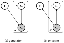
Figure 1: Graphical Models

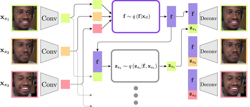
Figure 2: Model visualization

Generative Model: The generative model that describes the generation process above is given by

$$p_{\theta}\left(\mathbf{x}_{1:T},\mathbf{f},\mathbf{z}_{1:T}\right)=p_{\theta}\left(\mathbf{f}\right)\prod_{t=1}^{T}p_{\theta}\left(\mathbf{x}_{t}\>|\>\mathbf{f},\mathbf{z}_{t}\right)p_{\theta}\left(\mathbf{z}_{t}\>|\>\mathbf{f}\right),$$

where $\mathbf{f}$ and $\mathbf{z}_{t}$ are the latent variables that contain the static and dynamic information of each element, respectively. The parameters of the generative model are denoted as $\mathbf{\theta},$ and the RHS terms are formulated as follows:

$$p_{\theta}\left(\mathbf{f}\right) =\mathcal{N}\left(\mathbf{f}\>|\>\mathbf{0},\mathbf{1}\right),$$

$$p_{\theta}\left(\mathbf{z}\>|\>\mathbf{f}\right) =\mathcal{N}\left(\mathbf{z}\>|\>h_{\mu_{z}}\left(\mathbf{f}\right),\mbox{diag}\left(h_{\sigma^{2}_{z}}\left(\mathbf{f}\right)\right)\right)$$

$$p_{\theta}\left(\mathbf{x}\>|\>\mathbf{f},\mathbf{z}\right) =\operatorname{Ber}_{p}\left(\mathbf{x}\>|\>h_{x}\left(\mathbf{f},\mathbf{z}\right)\right),$$

where $p_{\theta}\left(\mathbf{f}\right)$ is a standard normal distribution and $p_{\theta}\left(\mathbf{z}\>|\>\mathbf{f}\right)$ is a multivariate normal distribution, parameterized by two neural networks $h_{\mu_{z}}$ and $h_{\sigma^{2}_{z}}.$ The likelihood $p_{\theta}\left(\mathbf{x}\>|\>\mathbf{f},\mathbf{z}\right)$ is a Bernoulli distribution parameterized by a neural network $h_{x}$. Experimentally, this leads to sharper results than using a Normal distribution.

Inference Model: To overcome the problem of intractable inference with the true posterior, we define an approximate inference model, $q_{\phi}\left(\mathbf{f},\mathbf{z}_{1:T}\>|\>\mathbf{x}_{1:T}\right).$ We train the generative model within the VAE framework proposed by Kingma and Welling (2013).

To successfully separate the static from the dynamic information, the model needs to know which information is common among $\mathbf{x}_{1:T}$. While a sequence could be arbitrary long, we randomly sample $N$ frames, $\mathbf{x}_{S}=\left(x_{s_{1}},\dots,x_{s_{N}}\right),$ from the sequence, whose pairwise comparison helps us compute the encoding for the static information $\mathbf{f}$.

We now consider the factorized inference model as depicted in Figure (2b):

$$q_{\phi}\left(\mathbf{f},\mathbf{z}_{s_{1:N}}|\mathbf{x}_{S}\right) =q_{\phi}\left(\mathbf{f}\>|\>\mathbf{x}_{S}\right)\prod_{i=1}^{N}q_{\phi}\left(\mathbf{z}_{s_{i}}\>|\>\mathbf{f},\mathbf{x}_{s_{i}}\right)$$

$$q_{\phi}\left(\mathbf{f}\>|\>\mathbf{x}_{S}\right) =\mathcal{N}\left(\mathbf{f}\>|\>g_{\mu_{f}}\left(\mathbf{x}_{S}\right),\mbox{diag}\left(g_{\sigma^{2}_{f}}\left(\mathbf{x}_{S}\right)\right)\right)$$

$$q_{\phi}\left(\mathbf{z}\>|\>\mathbf{f},\mathbf{x}\right) =\mathcal{N}\left(\mathbf{z}\>|\>g_{\mu_{z}}\left(\mathbf{f},\mathbf{x}\right),\mbox{diag}\left(g_{\sigma^{2}_{z}}\left(\mathbf{f},\mathbf{x}\right)\right)\right),$$

where the posteriors over $\mathbf{f}$ and $\mathbf{z}$ are multivariate normal distributions parameterized by neural networks $g_{\mu_{z}}\left(\mathbf{f},\mathbf{x}\right)$ and $g_{\sigma^{2}_{z}}\left(\mathbf{f},\mathbf{x}\right)$. The inference model parameters are denoted by $\phi.$

In the inference model $q\left(\mathbf{f}\>|\>\mathbf{x}_{S}\right)$ we learn the static information of $\mathbf{x}_{S}$. We achieve this by using the same convolutional layer for every concatenated pair of frames $\left(\mathbf{x}_{s_{j}},\mathbf{x}_{s_{i}}\right)\in\mathbf{x}_{S}.$ Through this architecture, the encoder learns only the common information of frames $\mathbf{x}_{S}$.

Learning: The variational lower bound for our model is given by

$$\mathcal{L} =\mathbb{E}_{q_{\phi}\left(\mathbf{f}\>|\>\mathbf{x}_{S}\right)}\left[\sum_{\mathbf{x}\in\mathbf{x}_{S}}\mathbb{E}_{q_{\phi}\left(\mathbf{z}\>|\>\mathbf{f},\mathbf{x}\right)}\left[\operatorname{log}p_{\theta}\left(\mathbf{x}\>|\>\mathbf{f},\mathbf{z}\right)-\operatorname{D}_{KL}\left(q_{\phi}\left(\mathbf{z}\>|\>\mathbf{f},\mathbf{x}\right)\>||\>p_{\theta}\left(\mathbf{z}\>|\>\mathbf{f}\right)\right)\right]\right]$$

$$\hskip 190.00029pt-\operatorname{D}_{KL}\left(q_{\phi}\left(\mathbf{f}\>|\>\mathbf{x}_{S}\right)\>||\>p_{\theta}\left(\mathbf{f}\right)\right),$$

which we optimize with respect to the variational parameters $\theta$ and $\phi.$

3 Related Work

Unsupervised learning of disentangled representations can be related to modeling context or hierarchical structure in datasets. In particular, our approach invites comparison to the “neural statistician” of Edwards and Storkey (2016), whose context variable closely corresponds to our static encoding, although our model has a different dependence structure.

On sequential data, Hsu et al. (2017) propose a factorized hierarchical variational auto-encoder using a lookup table for different means, while Li and Mandt (2018) condition a component of the factorized prior on the full ordered sequence. Denton and Birodkar (2017) use an adversarial loss to factor the latent representation of a video frame in a stationary and temporally varying component. Tulyakov et al. (2017) introduce a GAN that produces video clips by sequentially decoding a sample vector that consists of two parts: a sample from the motion subspace and a sample from a content subspace. In video generation, other directions can also be explored by decomposing the learned representation into deterministic and stochastic (Denton and Fergus (2018)).

fig:result1

Figure 3: Visualizations of learned dynamic data manifold of the two-dimensional latent space $\mathbf{z}$ for the MMNIST and Sprite dataset.

4 Experiments

We evaluate our model on two synthetic datasets Sprites (Li and Mandt (2018)) and Moving MNIST (Srivastava et al. (2015)), and a real one, Aff-Wild dataset (Kollias et al. (2018)). The detailed description of the preprocessing on these datasets is provided in appendix.

fig:result2

Figure 6: (a) Visualizations of learned dynamic data manifold of the two-dimensional latent space $\mathbf{z}$ for the AFF-Wild dataset (b) Plot of the first dimension of the encoded dynamics of video frames for a single sequence with some of the corresponding frames.

Qualitative evaluation For all models in this section we use $N=3$ frames and a batch size of 120. We set the dimension of the latent space $\mathbf{z}$ for the dynamic information to $2$. We used ADAM with learning rate $1e^{-4}$ to optimize the variational lower bound $\mathcal{L}$. To show the learned dynamics of the sequences of the datasets, we fix $\mathbf{f}$ and visualize the decoded samples from the grid in the latent space $\mathbf{z}$ (Fig. LABEL:fig:result1). In the case of the MMNIST, the digits and style of the handwritten numbers are consistent over the spanned space. The encoded dynamic can be interpreted as the position and orientation of the digits. Similar observation holds for the sprites dataset, but this time $\mathbf{z}$ encode the pose of the character. In both cases we can note the coherence of the dynamic space between different identities.

Application: Even with just two dimensions, the latent space $\mathbf{z}$ captures the dynamics of faces well, suggesting that it can be used for representing and analyzing expressions in an unsupervised way. To illustrate this concept, we plot one of the dynamic components of a sequence (Figure LABEL:fig:timeline). A naive analysis of this dynamic plot can already extract some meaningful facial expressions from a specific person. In this specific example, expressions we would call smiling and astonished.

5 Discussion

In this work, we introduced a deep generative model that effectively learns disentangled static and dynamic representations from data without temporal ordering. The ability to learn from unordered data is important as one can take advantage of the combinatorics of randomly choosing pairwise comparisons, to train models on small datasets. While in the current model the same frames are used to compute both the dynamic and static encodings, an interesting subject for future work would be to see if defining a distinct set of frames for the dynamic part would lead to a better separation.

Appendix A Details of experimental setup

Moving MNIST: We downloaded the public available preprocessed dataset from their website . It consists of sequences of length $20$ where each frame is of size $64\times 64\times 1$. For the model we learned on the MMNIST dataset, we set the dimension for the static information $\mathbf{f}$ to $64$ and trained it for 60k iterations.

Sprites: To create this dataset, we followed the same procedure as described in Li and Mandt (2018). We downloaded the available sheets from the github-repo and chose 4 attributes (skin color, shirt, legs and hair-color) to define a unique identity. For each of this attributes we selected 6 different appearances which makes in total $6^{4}=1296$ different combinations of identities. Although, instead of using a single instance of an action sequence, we used the whole sheet which consists of 178 different poses. The size of a single image is $64\times 64$. For the Sprite dataset we increased the dimensions for the latent space $\mathbf{f}$ to $256$ and trained it for 43k iterations.

Aff-Wild: The real world dataset is a preprocessed and normalized version of the Aff-Wild dataset Kollias et al. (2018). The dataset consists of 252 sequences, of length between 20 and 450 frames. Instead of using the whole video frame, we cropped the face and resized it to a size of $64\times 64$.

Appendix B Details of the encoder for the static latent variable model

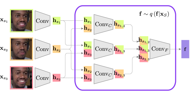
Figure 9: Visualization of the encoder for the static latent variable model

Appendix C Network Architecture

Conv: $\mathbf{x}_{s_{i}}\to\mathbf{h}_{s_{i}}$
{ conv2d: kernel: 4x4, filters: 256, stride: 2x2, activation: leaky ReLU }
{ conv2d: kernel: 4x4, filters: 256, stride: 2x2, activation: leaky ReLU }
{ conv2d: kernel: 4x4, filters: 256, stride: 2x2, activation: leaky ReLU }
{ conv2d: kernel: 4x4, filters: 256, stride: 2x2, activation: leaky ReLU }

$\textit{Conv}_{C}$: $\operatorname{concat}\left([\mathbf{h}_{s_{i}},\mathbf{h}_{s_{j}}]\right)\to\mathbf{h}_{s_{i,j}}$

{ conv2d: kernel: 3x3, filters: 512, stride: 1x1, activation: ReLU }

$\textit{Conv}_{F}$: $\operatorname{concat}\left([\mathbf{h}_{s_{1,2}},\mathbf{h}_{s_{1,3}},\mathbf{h}_{s_{2,3}}]\right)$ $\to$ [$\mu_{f}$, $\sigma^{2}_{f}$]
{ conv2d: kernel: 3x3, filters: 512, stride: 1x1, activation: ReLU }
{ dense: units: 512, activation: ReLU }
{ dense: units: 1024, activation: None }

$q_{\phi}\left(\mathbf{z}_{s_{i}}\>|\>\dots\right)$: $\operatorname{concat}\left([\mathbf{f},\mathbf{h}_{s_{i}}]\right)$ $\to$ [$\mu_{z}$, $\sigma^{2}_{z}$]
{ dense: units: 512, activation: ReLU }
{ dense: units: 512, activation: ReLU }
{ dense: units: 4, activation: None }

$\textit{p}_{\theta}\left(\mathbf{z}_{s_{i}}\>|\>\mathbf{f}\right)$: $\mathbf{f}\to$ [$\mu_{z}$, $\sigma^{2}_{z}$]
{ dense: units: 512, activation: ReLU }
{ dense: units: 512, activation: ReLU }
{ dense: units: 4, activation: None }

Deconv: $\operatorname{concat}\left([\mathbf{f},\mathbf{z_{s_{i}}}]\right)$ $\to$ $\tilde{\mathbf{x}}_{s_{i}}$
{ deconv2d: kernel: 4x4, filters: 256, stride: 2x2, activation: leaky ReLU }
{ deconv2d: kernel: 4x4, filters: 256, stride: 2x2, activation: leaky ReLU }
{ deconv2d: kernel: 4x4, filters: 256, stride: 2x2, activation: leaky ReLU }
{ deconv2d: kernel: 4x4, filters: 3, stride: 2x2, activation: None }

References

- Denton and Fergus (2018) Emily Denton and Rob Fergus. Stochastic video generation with a learned prior. CoRR, abs/1802.07687, 2018.
- Denton and Birodkar (2017) Emily L. Denton and Vighnesh Birodkar. Unsupervised learning of disentangled representations from video. In NIPS, pages 4417–4426, 2017.
- Edwards and Storkey (2016) Harrison Edwards and Amos J. Storkey. Towards a neural statistician. CoRR, abs/1606.02185, 2016.
- Hsu et al. (2017) Wei-Ning Hsu, Yu Zhang, and James R. Glass. Unsupervised learning of disentangled and interpretable representations from sequential data. In NIPS, pages 1876–1887, 2017.
- Kingma and Welling (2013) Diederik P. Kingma and Max Welling. Auto-encoding variational bayes. CoRR, abs/1312.6114, 2013.
- Kollias et al. (2018) Dimitrios Kollias, Panagiotis Tzirakis, Mihalis A. Nicolaou, Athanasios Papaioannou, Guoying Zhao, Björn W. Schuller, Irene Kotsia, and Stefanos Zafeiriou. Deep affect prediction in-the-wild: Aff-wild database and challenge, deep architectures, and beyond. CoRR, abs/1804.10938, 2018.
- Li and Mandt (2018) Yingzhen Li and Stephan Mandt. Disentangled sequential autoencoder. In ICML, volume 80 of JMLR Workshop and Conference Proceedings, pages 5656–5665. JMLR.org, 2018.
- Srivastava et al. (2015) Nitish Srivastava, Elman Mansimov, and Ruslan Salakhutdinov. Unsupervised learning of video representations using lstms. In ICML, volume 37 of JMLR Workshop and Conference Proceedings, pages 843–852. JMLR.org, 2015.
- Tulyakov et al. (2017) Sergey Tulyakov, Ming-Yu Liu, Xiaodong Yang, and Jan Kautz. Mocogan: Decomposing motion and content for video generation. CoRR, abs/1707.04993, 2017.