Sharp phase transition for random loop models on trees

Abstract

We investigate the random loop model on the $d$-ary tree. For $d\geq 3$, we establish a (locally) sharp phase transition for the existence of infinite loops. Moreover, we derive rigorous bounds that in principle allow to determine the value of the critical parameter with arbitrary precision. Additionally, we prove the existence of an asymptotic expansion for the critical parameter in terms of $d^{-1}$. The corresponding coefficients can be determined in a schematic way and we calculate them up to order $6$.

1 Introduction

Let $G=(V,E)$ be an undirected (simple) graph and let $\mathop{\mathbb{T}_{\beta}}:=\mathbb{R}/\beta\mathbb{Z}$ be the one-dimensional torus with length $\beta>0$. A link configuration on $E\times\mathop{\mathbb{T}_{\beta}}$ is a family $X=(X^{e,\star})_{e\in E,\star\in\{\mathop{\backslash\mathllap{/}},\mathop{||}\}}$ of measures on $\mathop{\mathbb{T}_{\beta}}$, such that $X^{e,\mathop{\backslash\mathllap{/}}}+X^{e,\mathop{||}}$ is a simple and finite atomic measure on $\mathop{\mathbb{T}_{\beta}}$ for each $e$, i.e. it is a finite sum of Dirac measures $\delta_{t_{i}}$ with $t_{i}\neq t_{j}$ when $i\neq j$. The atoms of $X^{e,\star}$ are called links and each link of $X$ is specified by a triple $(e,t,\star)$, where $\star\in\{\mathop{\backslash\mathllap{/}},\mathop{||}\}$ is the type and $t$ the position/time of the link on the edge $e$.

Each link configuration induces a loop configuration, which is a collection of open subsets of the set $V\times\mathop{\mathbb{T}_{\beta}}$. The rigorous definition of the map from a link configuration to a loop configuration, which will be given shortly, is a bit technical; its essence however can be conveniently grasped from Figure 1: A link of type $\mathop{\backslash\mathllap{/}}$ on an edge connects those regions on $\mathop{\mathbb{T}_{\beta}}$ on the two vertices adjacent to its edge that are on opposing sides of its position, while a link of type $\mathop{||}$ connects regions on the same side of its position. Regions on the same vertex are always separated by links on adjacent edges. After extension by transitivity, this yields a partition of $V\times\mathop{\mathbb{T}_{\beta}}$ into the closed set $\{(x,t):x\in V,t\in\mathop{\operatorname{supp}}X^{e,\star}\text{ for some }e\ni x,\star\in\{\mathop{\backslash\mathllap{/}},\mathop{||}\}\}$, and the open sets of mutually connected points (the loops).

The relevant quantity for loop models is the size of typical loops (in our case measured in the number of visited vertices, although the arc length is also a conceivable quantity of interest) when the link configuration is random. More precisely, the question is whether a given family of loop models has a percolation phase transition in the parameter $\beta$, i.e. whether (for an infinite graph) the probability that a given fixed vertex is contained in an infinite loop is positive for some $\beta$ and zero for others. The apparently simplest case is $G=\mathbb{Z}^{d}$, $X^{e,\mathop{||}}=0$ for all edges $e$ and the $X^{e,\mathop{\backslash\mathllap{/}}}$ are iid Poisson point processes of rate $1$. While numerical results [5] strongly suggest the existence of a phase transition, on a rigorous level the question is completely open in this case.

The main difficulty in the loop model is the lack of monotonicity, i.e. more links do not necessarily mean longer loops. This can already be seen in Figure 1: removing one of the links between the two middle vertices merges the red and blue loop into one. Moreover, local changes of the loop configuration can connect or disconnect intervals in very different regions of $G$, so the model is highly non-local in this sense. These two obstacles have so far prevented the development of efficient tools to investigate percolation on loop models on most graphs, leading to a relative scarcity of results; however, a few results exist, and we will review them now.

Figure 1: Example of a small finite graph $G$ and a link configuration $X$ (left) leading to the two depicted loops (right, red and blue).

In the context of probability theory, the loop model goes back to the random stirring process, introduced by Harris [18]. This process $(\sigma_{t})_{t\in[0,\beta]}$ of permutations on $V$ corresponds to the random loop model mentioned above, i.e. with $X^{e,\mathop{||}}=0$ and $X^{e,\mathop{\backslash\mathllap{/}}}$ iid Poisson point processes. Namely, given a link configuration $X$ and setting $\sigma_{0}$ to be the identity permutation, we increase time $t$ and if there is a link on an edge $\{x,y\}$ at the position $t$ that we currently consider, we compose $\sigma_{t-}$ with the transposition of $x$ and $y$. It is easy to see that two vertices $x$ and $y$ are contained within the same cycle of $\sigma_{\beta}$ iff $(x,0)$ and $(y,0)$ share a loop.
Note that, on arbitrary connected graphs with bounded degree, the critical parameter $\beta_{c}$ is strictly larger than the percolation threshhold for edges carrying at least one link [22]. For the random stirring model on the (finite) complete graph, the phase transition occurs at $\beta_{c}=|V|^{-1}$ in the limit of $|V|\to\infty$, see e.g. [6, 7]. Moreover, for a time-discrete model where one link occurs at each step and for time-scales above a critical value corresponding to $\beta_{c}=|V|^{-1}$ in our setting, Schramm showed in [23] that the distribution of cycle sizes within the giant component converges (after renormalisation) to a Poisson-Dirichlet distribution of parameter $1$. In [10], this result has been extended to include links of type $\mathop{||}$, too.
Apart from the complete graph and the $2$-dimensional Hamming graph [21], another graph for which progress has been made in the context of the random stirring model is the $d$-ary tree. Angel [3] showed the existence of two different phases for $d\geq 4$, and the existence of infinite cycles for $\beta\in(d^{-1}+\tfrac{13}{6}d^{-2},\ln(3))$ in the asymptotic regime $d\to\infty$. Hammond then showed in [15] that (for $d\geq 2$) there is a value $\beta_{0}$ above which $\sigma_{\beta}$ contains infinite cycles and that for $d\geq 55$, one may chose $\beta_{0}=101d^{-1}$. Furthermore and for even larger $d$, strict bounds for this critical parameter have been found in [16] and it was shown that the transition from finite to infinite cycles is sharp. In the recent work of Hammond and Hegde [17], these bounds have been proven to hold for $d\geq 56$ while even including links of type $\mathop{||}$. Moreover, Björnberg and Ueltschi [11] determined the critical parameter $\beta_{c}$ of the loop model up to second order in $d^{-1}$ as $d\to\infty$. The reader should note that the majority of the above results rely on graph degrees being comparatively large, or are even just asymptotic in them.

In the present paper we significantly improve the existing results for $d$-ary trees and achieve a rather complete picture of the random loop model in these cases. We focus on the case where the $(X^{e,\star})$ are iid Poisson point processes, but it should be clear how our method extends to other families of independent point processes. While a simple percolation argument shows that almost surely there are no infinite loops for $\beta\leq d^{-1}$, our methods aim at the critical region $d^{-1}<\beta\leq d^{-1/2}$. In Theorem 2.1 below, we establish the existence of a sharp phase transition for all $d\geq 3$ within this region, comparable results previously existed only up to $d^{-1}+2d^{-2}$ and for $d\geq 26$ [17]. Additionally, in Theorem 2.2, we provide an asymptotic expansion of the critical value in powers of $1/d$, with coefficients depending on the parameter $u$ controlling the relative intensities of the point processes $X^{e,\mathop{\backslash\mathllap{/}}}$ and $X^{e,\mathop{||}}$.

Our proofs rely on a natural idea: the central object are those edges that carry precisely one link. It is not difficult to see that at such edges a renewal event occurs: Removing any edge $e$ splits the tree $G$ into two disconnected subtrees $G_{1}$ and $G_{2}$. Thus, in the case that $e$ only carries a single link, and if the loop through that link is finite on $G_{1}$, say, then that loop has to pass through $e$ in both directions. Consequently, in this case the loop structure on $G_{2}$ depends only on the link structure of $G_{2}$ and not on the link structure on $G_{1}$. This allows to construct renewal schemes that use single-link edges as ‘new roots’.

The first such renewal scheme was presented in the work of Angel [3]. The paper uses a single-link edge $e=\{x,y\}$ as a renewal edge if the arrival time $t_{e}$ of its link is uncovered, meaning that none of its siblings has a pair of links whose arrival times separate the time $t_{e}$ of the link on $e$ from the first time the loop meets the parent $x$ of $e$, in the topolgy of the torus $\mathbb{T}_{\beta}$. This guarantees that any loop arriving at the parent $x$ of $e$ either is already infinite or will eventually pass through $e$. The proof then consists in identifying conditions under which infinitely many renewal edges exist with positive probability. The main limitation of this scheme is that being uncovered is a rather strong restriction on a single-link edge, and that an un-interrupted chain of uncovered edges is needed from the root to infinity with positive probability. Thus the criterion leads to conditions that are far from optimal. In particular they are only accurate to first order in $1/d$ for large $d$, and only work for $d\geq 4$.

Our approach is a more systematic one: we consider multilink-clusters, i.e., the finite subtrees of the infinite tree whose edges all have more than one link, and use as renewal edges all single-link edges protruding from these subtrees that carry the loop entering the subtree at its root. In comparison to the method of [3], this allows not only for covered single-link edges to be used, but it (in principle) allows us to cross any number of edges that have multiple links.

One limitation that our method does have is that it relies on a sufficiently high probability for the multilink-cluster to be finite. This poses no limitation for $\beta\leq d^{-1/2}$ as this is below the percolation threshold for these clusters, but becomes an obstacle for higher $\beta$. Since $\beta_{c}\sim 1/d$ for large $d$, no problem appears in view of the asymptotic estimates for $\beta_{c}$, and in the regime of small $d$ our results are sufficient to identify $\beta_{c}$ with high precision. However, for the proof that there is no phase of almost surely finite loops beyond $\beta_{c}$, we need to rely on results obtained by Hammond and Hegde [17]. It is not inconcievable that this could be improved by suitable lower bounds for the expected number of renewal edges for an infinite (or very large) multilink-cluster, but such an investigation is beyond the scope of the current work and left for future investigations.

Apart from random stirring, a strong motivation for studying random loop models comes from their relation to quantum mechanical models. More precisely, in [2] and [24] stochastic representations of the spin-$\tfrac{1}{2}$ quantum Heisenberg antiferromagnet and ferromagnet, respectively, were studied. Recently, Ueltschi [25] introduced the random loop model as a common generalisation that interpolates between those representations and also includes a representation of the spin-$\tfrac{1}{2}$ XY model. For these representations, each link configuration receives a weight proportional to $\theta^{\#\text{loops}}$, so for $\theta\neq 1$, links on different edges are no longer independent. Also, the model cannot be directly defined on an infinite graph. Thus, it has to be constructed via an infinite volume limit. Physcially, $\theta=2$ is the most relevant case. The occurrence of infinite loops is then related to non-decay of correlations for the quantum spin systems. Therefore, in order to see that these systems undergo a phase transition and to determine the critical inverse temperature $\beta_{c}$ at which it occurs, one possibility is to investigate the different phases of the random loop model.
As it is the case in the random stirring model, the most interesting (but also apparently the most challenging) graph to study these models on is $\mathbb{Z}^{d}$. Mathematical results exist for the complete graph [9, 13], the $2$-dimensional Hamming graph [1], Galton-Watson trees [8] and the $d$-ary tree [12], again in the regime of high degrees. Unfortunately, for $\theta\neq 1$, the weighted measures involve intricate correlations and the techniques of our paper do not directly apply.

This paper is organized as follows: In Section 2, we state our precise assumptions and results. In Section 3, we introduce exploration schemes, a recursive construction with a renewal structure that constitutes the core of our proof as it gives a Galton-Watson process whose survival is related to the event that the loop containing the root at time $0$ is infinite. This enables us to distinguish the phases by considering the expected value for the first generation of this process and without much further work, we are then already able to establish a locally sharp phase transition for all $d\geq 5$. Afterwards, within Section 4, we will turn our attention to the asymptotic expansion and on the way to its proof, we will discover sufficient (and computable) conditions for the two phases. Finally, in Section 5, we will then establish the necessary computations that enable us to push our results to $d=3$ and to calculate coefficients within the asymptotic expansion.

2 Main results

We start by giving a proper definition of the map from link configurations to loop configurations. Suppose that $X=(X^{e,\star})_{e\in E,\star\in\{{\mathop{\backslash\mathllap{/}}},{\mathop{||}}\}}$ is a link configuration. We call $X$ admissible if $X^{e,\star}$ and $X^{e^{\prime},\star^{\prime}}$ are mutually singular whenever $e\neq e^{\prime}$ but $e\cap e^{\prime}\neq\emptyset$, and also when $e=e^{\prime}$ and $\star\neq\star^{\prime}$. This guarantees that the construction of loops given below is well defined. When fixed link configurations are given, we will always assume that they are admissible, and that all our link-configuration-valued random variables will produce admissible link configurations almost surely.

Given an admissible link configuration $X$, a loop is an equivalence class of elements of $V\times\mathop{\mathbb{T}_{\beta}}$ induced by the following connectedness relation: We equip $V$ with the discrete and $\mathop{\mathbb{T}_{\beta}}$ with the quotient topology and say that two points $(x_{0},t_{0})$ and $(x_{1},t_{1})\in V\times\mathop{\mathbb{T}_{\beta}}$ are connected iff there is no link on an edge incident to $x_{i}$ at position $t_{i}$, $i=0,1$, and there is a piecewise continuous path $\Gamma=(\Gamma_{1},\Gamma_{2})\colon[0,1]\to V\times\mathop{\mathbb{T}_{\beta}}$ from $(x_{0},t_{0})$ to $(x_{1},t_{1})$ such that

• $\Gamma_{2}$ is continuous everywhere and differentiable at every point of continuity of $\Gamma$. Where the derivative $\Gamma_{2}^{\prime}$ exists, its absolute value is a fixed constant.

• If $\Gamma$ is discontinuous at $s\in(0,1)$, then there is a link on $\{\Gamma_{1}(s-),\Gamma_{1}(s+)\}$ at position $\Gamma_{2}(s)$.

• For all links $(\{x,y\},t,\star)$ of $X$ such that $\Gamma(s-)=(x,t)$ (or $\Gamma(s+)=(x,t)$) for some $s\in(0,1)$ we have $\Gamma(s+)=(y,t)$ (or $\Gamma(s-)=(y,t)$, respectively) as well as

  $$\Gamma_{2}^{\prime}(s+)=\left\{\begin{array}[]{cl}+\Gamma_{2}^{\prime}(s-)&\text{ if }\star=\mathop{\backslash\mathllap{/}},\\ -\Gamma_{2}^{\prime}(s-)&\text{ if }\star=\mathop{||}.\end{array}\right.$$

Note that a loop $\gamma$ is by definition a subset of $V\times\mathop{\mathbb{T}_{\beta}}$. Nevertheless, in a slight abuse of notation, we write $x\in\gamma$ iff there is a $t\in\mathop{\mathbb{T}_{\beta}}$ with $(x,t)\in\gamma$. Similarly, we set

$$|\gamma|:=|\{x\in V:x\in\gamma\}|.$$

Now that we have defined loops, let us fix our assumptions. We write $T=(V,E)$ for the $d$-ary tree with root $r\in V$, i.e. the tree where each vertex has $d$ ‘children’ and (except for $r$) one ‘parent’. We assume that the link configuration is given by an independent family $(X^{e,\star})_{e\in E,\star\in\{\mathop{\backslash\mathllap{/}},\mathop{||}\}}$ of homogeneous Poisson point processes, where for each $e\in E$, $X^{e,\mathop{\backslash\mathllap{/}}}$ has rate $u\in[0,1]$ and $X^{e,\mathop{||}}$ has rate $1-u$. Under these assumptions, we have:

Theorem 2.1 (Existence and local sharpness of the phase transition).

  
Let $\gamma_{T}$ be the loop on $T$ containing $(r,0)$. Then for all $d\geq 3$ and for all $u\in[0,1]$ there exist $\mathop{\beta^{*}}\geq d^{-1/2}$ and $\beta_{c}\in(0,\mathop{\beta^{*}})$ such that

1. $|\gamma_{T}|<\infty$ almost surely for all $\beta\leq\beta_{c}$,

2. $|\gamma_{T}|=\infty$ with positive probability for all $\beta\in(\beta_{c},\mathop{\beta^{*}})$.

Note that, for $d=1$, there is no phase transition since $|\gamma_{T}|<\infty$ almost surely (non-zero probability of empty edges). Moreover, the case $d=2$ technically is accessible with our method. However, it would take much more computational effort to prove a similar statement in this case, see Remark 5.5. Furthermore note that a re-entry into the phase of finite loops for $\beta>d^{-1/2}$ is quite implausible. Nevertheless, we cannot exclude this behaviour as our method is tailored for $\beta$ up to $d^{-1/2}$. Still, in combination with [17, Proposition 1.2 (2),(4)], Theorem 2.1 suffices to show that there is no re-entry and that the phase transition is thus globally sharp for all $d\geq 16$, therefore improving the previously known lower bound of $d\geq 56$ from [17].

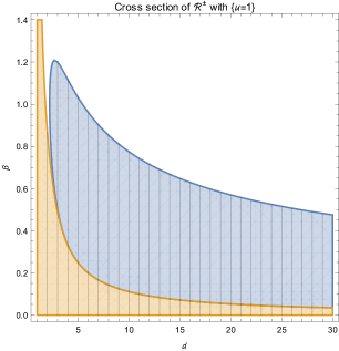
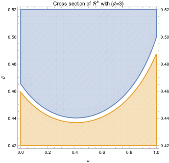
Figure 2: Regions $\mathcal{R}_{5}^{\pm}$ of parameters $(\beta,d,u)$ where we can guarantee that $\gamma_{T}$ is infinite with positive probability (upper/blue region $\mathcal{R}^{+}_{5}$) and that $\gamma_{T}$ is finite almost surely (lower/sandybrown region $\mathcal{R}^{-}_{5}$), respectively. See (4.2) and (4.3) for a precise definition of these regions.

In addition to establishing a phase transition, the tools we develop also yield an equation in $\beta$ that is solved by $\beta_{c}$, compare Proposition 3.6 and (3.3). We may then approximate its terms systematically to find sharp bounds on the critical parameter $\beta_{c}$ for every $d\geq 3$. These estimations rely on solving a certain combinatorial problem associated to finite edge-weighted trees, giving implicit conditions about the phase regions. Instead of providing explicit but imprecise bounds for $\beta$ (which would also be possible, cf. (2.3)), we rather check whether one of these implicit conditions is satisfied. Thereby, we obtain a region of parameters $(\beta,d,u)$ where $\gamma_{T}$ is infinite with positive probability (blue region in Figure 2) and a region where it is finite almost surely (sandybrown region in Figure 2). The critical parameter $\beta_{c}$ thus lies within the small (white) gap between these regions. For more details on these implicit conditions and the corresponding combinatorial problem, we refer to Lemma 4.1 and Section 5.

A further analysis of the terms within the determining equation for $\beta_{c}$ yields the following result.

Theorem 2.2 (Asymptotic expansion of $\beta_{c}$).

There exist polynomials $\alpha_{0},\alpha_{1},\alpha_{2},\ldots$ such that for any $K\in\mathbb{N}_{0}$ the critical parameter is asymptotically given by

$$\beta_{c}=\sum_{k=1}^{K+1}\frac{\alpha_{k-1}(u)}{d^{k}}+\mathcal{O}(d^{-(K+2)})$$ (2.1)

as $d\to\infty$.

In fact, we know somewhat more than just the existence of the polynomials $\alpha_{0},\ldots,\alpha_{K}$: the degree of $\alpha_{k}$ is at most $2k$ and each $\alpha_{k}$ is explicitly given in terms of $\alpha_{0},\ldots,\alpha_{k-1}$ as well as derivatives of a function $F_{k}$, see (4.6). However, the evaluation of $F_{k}$ relies on solving the aforementioned combinatorial problems associated with fixing the multilink-cluster and the total number of links on its edges such that the difference between this number of links and the number of edges is at most $k$. Thus, it becomes increasingly time-consuming to determine $F_{k}$ as $k$ increases and we have implemented this computation up to $K=5$. In particular, we find that $\alpha_{0}$ and $\alpha_{1}$ coincide with the result of [11]. Interestingly, the polynomials that we found exhibit an intriguing property: they are convex functions of $u$, and writing $\alpha_{k}$ with respect to the basis of Bernstein polynomials of degree $2k$, i.e.

$$\alpha_{k}(u)=\sum_{j=0}^{2k}\alpha_{k,j}{{2k}\choose{j}}u^{j}(1-u)^{2k-j},$$ (2.2)

their coefficients satisfy $0<\alpha_{k,j}\leq 1$ for all $j$ and all $k\leq 5$, see Table 1. Note that, for $k=1$, the occurrence of positive coefficients seems reasonable as $u^{j}(1-u)^{2-j}$ might account for the contribution of events with $j$ crosses and $2-j$ bars on the sole edge of the multilink-cluster. However, for $k\geq 2$, the combinatorial problems associated with three or more links on one edge of the multilink-cluster need to be included (compare with Table 2), but there is no corresponding basis polynomial. Therefore, this cannot explain this feature and hence, we do not know whether this structure persists for larger $k$ or, if it persists, what the reason is.

$\displaystyle\begin{array}[t]{c|cccccc}\alpha_{k,j}&k=0&k=1&k=2&k=3&k=4&k=5\\ \hline\cr j=0&1&5/6&2/3&1559/2520&7973/12960&375181/604800\\ j=1&&1/2&47/120&1451/3780&71693/181440&120203/297000\\ j=2&&1&28/45&6737/12600&621463/1270080&418041641/898128000\\ j=3&&&1/3&353/1260&46727/169344&70171259/239500800\\ j=4&&&11/12&1721/2700&4531/7938&122779529/232848000\\ j=5&&&&9/40&210167/1270080&122840869/838252800\\ j=6&&&&307/360&226769/317520&238710041/349272000\\ j=7&&&&&57/320&8806229/399168000\\ j=8&&&&&939/1120&28680241/35925120\\ j=9&&&&&&4541/28800\\ j=10&&&&&&62417/72576\end{array}$

Table 1: Coefficients $(\alpha_{k,j})_{j=0}^{2k}$ of the polynomial $\alpha_{k}$ with respect to the Bernstein basis polynomials of degree $2k$ for $k=0,\ldots,5$, compare (2.2).

In addition to the given asymptotic expansion, we may evaluate the aforementioned implicit conditions from Lemma 4.1 with sufficiently high numerical precision at suitable approximations for $\beta_{c}$ and, for instance, we find that

$$0\leq\beta_{c}-\sum_{k=1}^{3}\frac{\alpha_{k-1}(u)}{d^{k}}\leq\frac{2}{d^{4}}$$ (2.3)

for all $3\leq d\leq 100$ and $u\in[0,1]$.

3 The exploration scheme

The core object we will be working with is an exploration scheme, i.e., a map that assigns a sequence $(M_{n})_{n}$ with $M_{n}\subseteq V$ to each link configuration $X$. By construction, this process follows the propagation of the loop $\gamma_{T}$ through the tree and, in particular, the survival of $(M_{n})_{n}$ is related to the event that $|\gamma_{T}|=\infty$. Moreover, every $x\in M_{n}$ will have an ancestor within $M_{n-1}$ which is not necessarily the predecessor of $x$. Rather, given its ancestor, $x$ is chosen in a way such that the edge preceding $x$ carries one link that renews $\gamma_{T}$ in a certain way. From this renewal property and for $X$ given by Poisson point processes, it follows that $(|M_{n}|)_{n}$ is a Galton-Watson process and we may therefore characterise its survival probability by $\mathbb{E}(|M_{1}|)$. Fortunately, we can calculate this expected value quite well, resulting in both theorems from Section 2.

Before we may get into a detailed analysis, let us fix some notation. For $x,y\in V$, we write $x\sim y$ iff $\{x,y\}\in E$ and $y\geq x$ iff the unique shortest path from $y$ to the root contains $x$. A connected subgraph $S$ of $T$ with $x\in V(S)$ and $y\geq x$ for all $y\in S$ is called a subtree of $T$ with root $x$. Given such a subtree $S$ of $T$ with root $x$, we write $S^{+}$ for the enlargement of $S$ by one layer, i.e., $S^{+}$ is the subtree with edge set $E(S^{+})=\{e\in E:e\cap V(S)\neq\emptyset\text{ and }e\neq e_{x}^{-}\}$, and with vertex set $V(S^{+})=\{x\in V:x\in e\text{ for some }e\in E(S^{+})\}$. Here, for $x\neq r$, $e_{x}^{-}=\{\mathop{\operatorname{pred}}(x),x\}$ denotes the edge from $x$ to its predecessor $\mathop{\operatorname{pred}}(x)$. Moreover, for a subgraph $S\subseteq T$ and a link configuration $X$ on $T$, we obtain the link configuration $X_{S}$ by retaining only the links on edges of $S$. Additionally, if $S\subseteq T$ is a subtree, $x\in V(S)$ and $t\in\mathop{\mathbb{T}_{\beta}}$, we write $\gamma_{S,x,t}$ for the loop induced by $X_{S}$ on $S$ that contains $(x,t)$. In particular, if $r\in V(S)$, we write $\gamma_{S}=\gamma_{S,r,0}$ for brevity. Finally, we write $N^{e}:=X^{e,\mathop{\backslash\mathllap{/}}}(\mathop{\mathbb{T}_{\beta}})+X^{e,\mathop{||}}(\mathop{\mathbb{T}_{\beta}})$ for the total number of links on an edge $e\in E$.

The basic observation that our method is based on is the following renewal property.

Lemma 3.1.

Let $\{x,y\}\in E$ with $N^{\{x,y\}}=1$, i.e. $\mathop{\operatorname{supp}}(X^{\{x,y\},\mathop{\backslash\mathllap{/}}}+X^{\{x,y\},\mathop{||}})=\{t\}$ for some $t\in\mathop{\mathbb{T}_{\beta}}$. Denote by $S_{x}$ and $S_{y}$ the distinct subtrees of $T$ such that $x\in V(S_{x})$, $y\in V(S_{y})$, $V(S_{x})\cup V(S_{y})=V$ and $\{x,y\}\notin E(S_{x})\cup E(S_{y})$. Then for any loop $\gamma$ that crosses $\{x,y\}$, i.e. such that $\gamma\cap\{x\}\times U\neq\emptyset$ for any open neighbourhood $U$ of $t$, we have

$$\gamma\subseteq\gamma_{S_{x},x,t}\cup\gamma_{S_{y},y,t}.$$ (3.1)

Moreover, if $|\gamma|<\infty$, we even have equality within (3.1) except for the points $(x,t)$ and $(y,t)$.

Proof.

If $(x,t-)\in\gamma$, then we distinguish between two cases:

1. If $(x,t+)\in\gamma$, points in $V(S_{x})\times\mathop{\mathbb{T}_{\beta}}$ are connected according to $X$ if and only if they are connected according to $X_{S_{x}}$ – with the exception of the point $(x,t)$.

2. If $(x,t+)\notin\gamma$, there is no possibility for the connecting path to come back to $S_{x}$ as the underlying graph is a tree and the path needs a link to cross from $y$ to $x$. Thus, ignoring the link on $\{x,y\}$ will increase the set of points within $V(S_{x})\times\mathop{\mathbb{T}_{\beta}}$ that are connected.

The same argument holds if we initially had $(x,t+)\in\gamma$ (with $t-$ and $t+$ exchanged) and this shows (3.1). Moreover, if $\gamma$ is a finite loop, then it is closed, meaning that two points within $\gamma$ are connected by two distinct paths. Thus, since the underlying graph is a tree and in comparison with the link configuration $\tilde{X}$ one obtains from $X$ by removing the link on $\{x,y\}$, the addition of this link affects at most one of these paths. Therefore, the points $(x,t-)$ and $(x,t+)$ that were connected w.r.t. $\tilde{X}$ remain connected w.r.t. $X$, compare with [11, Proposition 2.2]. This means that the case (2) cannot occur for $|\gamma|<\infty$ and we obtain the asserted equality. ∎

Note that, in general, we do not know whether case (1) or (2) holds by just considering $X_{S_{x}}$. However, splitting a loop $\gamma(X)$ into $\gamma_{S_{x},x,t}(X_{S_{x}})$ and $\gamma_{S_{y},y,t}(X_{S_{y}})$ gives an upper bound for the propagation of $\gamma$ that is optimal in the sense that at least for $|\gamma|<\infty$ we have equality.

To apply this observation, assume that we are given a link configuration $X$ on $T$. Now, we explore the tree starting from the root and consider the multilink-cluster $\bar{C}_{x}$ rooted in some $x\in V$. That is, $\bar{C}_{x}$ is the maximal subtree with root $x$ such that each of its edges has at least two links, i.e.

$$\bar{C}_{x}:=\bigcup\{S\subseteq T:S\text{ subtree with root }x,N^{e}\geq 2\text{ for all }e\in E(S)\}.$$

If this subtree is infinite, we may not be able to apply Lemma 3.1 to divide the propagation of $\gamma_{T}$ into finite segments, therefore we set

$$C_{x}:=\begin{cases}\bar{C}_{x}&\text{ if }|\bar{C}_{x}|<\infty,\\ \emptyset&\text{ otherwise.}\end{cases}$$

The exploration scheme is then defined recursively by $M_{0}:=\{r\}$ and

$$M_{n+1} :=\bigcup_{x\in M_{n}}M_{1}^{x},\qquad n=0,1,2,\ldots$$

with

$$M_{1}^{x} :=\{y\in V(C_{x}^{+})\setminus V(C_{x}):y\in\gamma_{C_{x}^{+},x,t_{x}}\},$$

where $t_{r}=0$ and $\{t_{x}\}=\{t_{x}(X)\}:=\mathop{\operatorname{supp}}X^{e_{x}^{-}}$ for $x\neq r$. A sketch of these quantities is given in Figure 3.

Figure 3: On the $3$-ary tree, the numbers $N^{e}$ of links on the edges $e\in E$ constitute the multilink-cluster $C_{r}$. Whereever the loop $\gamma_{T}$ crosses an edge protruding from $C_{r}$, a vertex of $M_{1}$ occurs.

Note that, for $n\in\mathbb{N}$, there is always exactly one link on the edge $e_{x}^{-}$ preceding any $x\in M_{n}$. Therefore, we may indeed apply Lemma 3.1 to these edges and obtain that – if $\gamma_{T}$ is finite – the trace of $\gamma_{T}$ within $C_{x}^{+}$ coincides with $\gamma_{C_{x}^{+},x,t_{x}}$. Thus, $\gamma_{T}$ reaches the boundary vertices $V(C_{x}^{+})\setminus V(C_{x})$ of $C_{x}^{+}$ if and only if the loop $\gamma_{C_{x}^{+},x,t_{x}}$ does so and the latter information is encoded within $M_{1}^{x}$. On the other hand, if $\gamma_{T}$ is infinite, then $\gamma_{C_{x}^{+},x,t_{x}}$ is an upper bound for the trace of $\gamma_{T}$ within $C_{x}^{+}$. This allows us to relate the survival/extinction of $(M_{n})_{n}$ to the infiniteness/finiteness of $\gamma_{T}$.

Proposition 3.2.

Fix a link configuration $X$.

1. If $\left|\bigcup_{n\in\mathbb{N}_{0}}M_{n}\right|=\infty$, then $|\gamma_{T}|=\infty$.

2. If $\left|\bigcup_{n\in\mathbb{N}_{0}}M_{n}\right|<\infty$ and $|\bar{C}_{x}|<\infty$ for all $x\in\bigcup_{n\in\mathbb{N}_{0}}M_{n}$, then $|\gamma_{T}|<\infty$.

Proof.

Let us begin with two observations that hold for any $x\in\bigcup_{n}M_{n}$. On the one hand, for $y\in V(C_{x}^{+})\setminus V(C_{x})$ with $N^{e_{y}^{-}}=1$, we have $y\in M_{1}^{x}$ iff $(\mathop{\operatorname{pred}}(y),t_{y})\in\gamma_{C_{x},x,t_{x}}$. On the other hand, we may apply Lemma 3.1 to edges $\{e_{x}^{-}\}\cup\big{(}E(C_{x}^{+})\setminus E(C_{x})\big{)}$ to find

$$\gamma_{T}\,\cap\,V(C_{x})\times\mathop{\mathbb{T}_{\beta}}\subseteq\gamma_{C_{x},x,t_{x}}.$$ (3.2)

Moreover, for $|\gamma_{T}|<\infty$ we even have equality within (3.2) up to finitely many isolated points.
Now, to prove (a), suppose that $\bigcup_{n\in\mathbb{N}_{0}}M_{n}$ is infinite and pick a sequence $(x_{n})_{n\in\mathbb{N}_{0}}$ with $r=x_{0}\leq x_{1}\leq\ldots$ as well as $x_{n}\in M_{n}$ for all $n$. If we further assume that $|\gamma_{T}|<\infty$, we may set $n_{0}:=\max\{n:x_{n}\in\gamma_{T}\}$, $x:=x_{n_{0}}$ and $y:=x_{n_{0}+1}\in M_{1}^{x}$. Combining the two observations from the beginning of this proof, this gives $y\in\gamma_{T}$ – in contradiction to the maximality of $n_{0}$.
For (b), suppose that $|\gamma_{T}|=\infty$ and choose $(x_{k})_{k\in\mathbb{N}_{0}}\subseteq V$ with $r=x_{0}\leq x_{1}\leq\ldots$, $x_{0}\sim x_{1}\sim\ldots$ as well as $x_{k}\in\gamma_{T}$ for all $k$. If, however, $\bigcup_{n}M_{n}$ is finite, then there is $k_{0}:=\max\{k:x_{k}\in\bigcup_{n\in\mathbb{N}_{0}}M_{n}\}$. Thus, we may set $x:=x_{k_{0}}$ and $y:=x_{k_{1}+1}$, where $k_{1}:=\max\{k\geq k_{0}:x_{k}\in\bar{C}_{x}\}$ is finite by assumption. By the second preliminary observation, we find $(\mathop{\operatorname{pred}}(y),t_{y})\in\gamma_{C_{x},x,t_{x}}$ and thus $y\in M_{1}^{x}$ in contradiction to maximality of $k_{0}$. ∎

Now, let us assume that we are given link configurations at random. As mentioned before, for each realisation we may trace the (possible) propagation of $\gamma_{T}$ within the finite segments $C_{x}$ for some $x\in M_{n}$, $n\in\mathbb{N}_{0}$, by considering the loop $\gamma_{C_{x},x,t_{x}}$, and the random variables $M_{1}^{x}$ keep track where to start with new segments. Since this only relies on local information about $X$, it is no surprise that $(|M_{n}|)_{n}$ forms a Galton-Watson process under natural conditions on the distribution of $X$.

Lemma 3.3.

Let $(X^{e,\star})_{e\in E,\star\in\{{\mathop{\backslash\mathllap{/}}},{\mathop{||}}\}}$ be a family of admissible point processes on $\mathop{\mathbb{T}_{\beta}}$. Assume that the family $(X^{e,{\mathop{\backslash\mathllap{/}}}},X^{e,{\mathop{||}}})_{e\in E}$ is independent and identically distributed, and that each $X^{e,\star}$ is invariant under shifts in $\mathop{\mathbb{T}_{\beta}}$. Then $\bigcup_{n\in\mathbb{N}_{0}}M_{n}$ is infinite with positive probability if and only if $\mathbb{E}(|M_{1}|)>1$.

Proof.

To begin with, we have

$$\varphi_{n+1}(w)=\mathbb{E}\left(w^{|M_{n+1}|}\right)=\sum_{\Pi}\mathbb{E}\left(w^{|M_{n+1}|}\mathbf{1}_{\{M_{n}=\Pi\}}\right),$$

for $w\in[0,1]$, where $\varphi_{n}$ denotes the probability generating function of $|M_{n}|$ and where the sum runs over all subsets $\Pi$ of the leaves of some finite subtree of $T$. Now fix $\Pi$, let $S_{x}$ be the subtree of $T$ with root $x\in\Pi$ and set $S_{\Pi}:=T\setminus\bigcup_{x\in\Pi}S_{x}$ to be tree containing all remaining edges. Furthermore, for a realisation of $X$ within $\{M_{n}=\Pi\}$ we identify $X$ with $(X_{S_{\Pi}},(X_{S_{x}})_{x\in\Pi})$, where $X_{S}$ represents the links on edges $e\in E(S)$. Then, by definition, we have

$$|M^{x}_{1}(X)|=|M_{1}(\Theta_{x,t_{x}(X_{S_{\Pi}})}(X_{S_{x}}))|$$

for $x\in\Pi$. Here, $\Theta_{x,t}$ takes the links of $X_{S_{x}}$ and applies a position shift by $t$ as well as a spatial shift by some tree-isomorphism from $S_{x}$ to $T$ to these links. Since the first of these shifts leaves the distribution of $X_{S_{x}}$ invariant and the second maps it to the distribution of $X$, Fubini’s theorem implies

$$\varphi_{n+1}(w) =\sum_{\Pi}\mathbb{E}\left(\prod_{x\in\Pi}w^{|M_{1}^{x}|}\mathbf{1}_{\{M_{n}=\Pi\}}\right)$$

$$=\sum_{\Pi}\int\mathbb{P}(\mathrm{d}X_{S_{\Pi}})\mathbf{1}_{\{M_{n}=\Pi\}}(X_{S_{\Pi}})$$

$$\qquad\quad\prod_{x\in\Pi}\int\mathbb{P}(\mathrm{d}X_{S_{x}})w^{|M_{1}\circ\Theta_{x,t_{x}(X_{S_{\Pi}})}(X_{S_{x}})|}$$

$$=\sum_{\Pi}\mathbb{E}\left(\mathbb{E}(w^{|M_{1}|})^{|\Pi|}\mathbf{1}_{\{M_{n}=\Pi\}}\right)$$

$$=\mathbb{E}\left(\varphi_{1}(w)^{|M_{n}|}\right)=\varphi_{n}\circ\varphi_{1}(w).$$

Thus, by $\mathbb{P}(|M_{1}|=1)<1$ and since $|M_{n}|=0$ implies $|M_{n+1}|=0$, the standard (fixed-point) argument from the theory of Galton-Watson processes implies the asserted equivalence (compare [4, chapter I.3 and I.5]). ∎

Note that – with a little bit more effort – we could also show that $(|M_{n}|)_{n}$ is a Galton-Watson process. However, the stated characterisation of survival suffices for our purposes. In particular, by Proposition 3.2 and Lemma 3.3 it is clear that we need to be interested in ${\mathbb{E}}(|M_{1}|)$. For concreteness and because this is the most important situation, we only study this quantity in the case of the Poisson point processes described in the previous section.

For a concise presentation, we set

$$\begin{split}{\mathcal{S}}_{d}:=\{(S,n):&\;S\text{ is a finite subtree of }T\text{ with root }r,\\ &\;n\colon E(S)\to{\mathbb{N}_{0}}\text{ with }n(e)\geq 2\text{ for all }e\in E(S)\}.\end{split}$$

We also write the shorthand $n(S):=\sum_{e\in E(S)}n(e)$, $n!:=\prod_{e\in E(S)}n(e)!$ and define the event

$$A_{S,n}:=\{C_{r}=S\text{ and }N^{e}=n(e)\text{ for all }e\in E(S)\}$$

for $(S,n)\in\mathcal{S}_{d}$. By convention, we assume that $(S_{0},n_{0})\in\mathcal{S}_{d}$, where $S_{0}=(\{r\},\emptyset)$ is the trivial tree and where $n_{0}$ is the empty function with $n_{0}(S_{0})=0$.

Lemma 3.4.

Let $(X^{e,\star})_{e\in E,\star\in\{{\mathop{||}},{\mathop{\backslash\mathllap{/}}}\}}$ be independent homogeneous Poisson point processes on $\mathop{\mathbb{T}_{\beta}}$, with rate $u$ for $X^{e,{\mathop{\backslash\mathllap{/}}}}$ and $(1-u)$ for $X^{e,{\mathop{||}}}$. Then there exist nonnegative coefficients $p_{S,n}(d,u)$ (independent of $\beta$ and polynomial in $u$) with

$${\mathbb{E}}(|M_{1}|)=\sum_{(S,n)\in{\mathcal{S}}_{d}}\left({\mathrm{e}}^{-\beta d}(1+\beta)^{d-1}\right)^{|V(S)|}\beta^{n(S)+1}p_{S,n}(d,u).$$ (3.3)

For each $(S,n)\in\mathcal{S}_{d}$, the polynomials $p_{S,n}(d,u)$ can be calculated: Example 3.5 will deal with the most basic case and within Section 5, we will see how to reduce this calculation to a combinatorial problem for arbitrary $(S,n)$.

Proof of Lemma 3.4.

We decompose

$${\mathbb{E}}(|M_{1}|)=\sum_{(S,n)\in{\mathcal{S}}_{d}}{\mathbb{P}}\big{(}A_{S,n}\big{)}{\mathbb{E}}\big{(}|M_{1}|\,\big{|}\,A_{S,n}\big{)}.$$

By independence, and using also the facts that $|E(S^{+})\setminus E(S)|=d|V(S)|-|E(S)|$ and $|E(S)|=|V(S)|-1$, we find

$$\begin{split}{\mathbb{P}}\big{(}A_{S,n}\big{)}&=\prod_{e\in E(S)}{\mathbb{P}}(N^{e}=n(e))\prod_{e\in E(S^{+})\setminus E(S)}{\mathbb{P}}(N^{e}\leq 1)\\ &=\frac{\prod_{e\in E(S)}\beta^{n(E)}}{\prod_{e\in E(S)}n(e)!}{\mathrm{e}}^{-\beta|E(S)|}\big{(}(1+\beta){\mathrm{e}}^{-\beta}\big{)}^{d|V(S)|-|E(S)|}\\ &=\frac{\beta^{n(S)}}{n!}{\mathrm{e}}^{-\beta d|V(S)|}(1+\beta)^{(d-1)|V(S)|+1}.\end{split}$$

On the other hand,

$${\mathbb{E}}\big{(}|M_{1}|\,\big{|}\,A_{S,n}\big{)}=\sum_{y\in V(S^{+})\setminus V(S)}{\mathbb{P}}\big{(}y\in\gamma_{S^{+}}\,\big{|}\,A_{S,n}\big{)},$$

and the term in the sum on the right hand side above can be written as

$${\mathbb{P}}\big{(}y\in\gamma_{S^{+}}\,\big{|}\,A_{S,n},N^{e_{y}^{-}}=1\big{)}{\mathbb{P}}\big{(}N^{e_{y}^{-}}=1\,\big{|}\,A_{S,n}\big{)},$$

where we used that $y\in\gamma_{S^{+}}$ implies $N^{e_{y}^{-}}=1$. Now, for all $y$, the second factor above is equal to ${\mathbb{P}}(N^{e_{y}^{-}}=1|N^{e_{y}^{-}}\leq 1)=\frac{\beta}{1+\beta}$ by independence. Moreover, the first factor does not depend on $\beta$: By

$$\{y\in\gamma_{S}^{+},N^{e_{y}^{-}}=1\}\cap A_{S,n}=\{(\mathop{\operatorname{pred}}(y),t_{y})\in\gamma_{S},N^{e_{y}^{-}}=1\}\cap A_{S,n},$$

we see that the event depends on the link configuration on edges $e\in E(S)\cup\{e_{y}^{-}\}$ and for these edges, the total number $N^{e}$ of links on each $e$ is fixed. By regarding, for each edge $e$, the random variables $(X^{e,\star})_{\star\in\{\mathop{\backslash\mathllap{/}},\mathop{||}\}}$ as the result of first determining the total number of links on $e$ by a Poisson random variable with expectation $\beta$, then determining their type by a Bernoulli random variable with success probability $u$, and then determining the position of their link(s) by a uniform random variable on $\{(s_{1},\ldots,s_{N^{e}})\in\mathbb{T}_{\beta}^{N^{e}}:s_{1}\leq\ldots\leq s_{N^{e}}\}$, one sees that ${\mathbb{P}}((\mathop{\operatorname{pred}}(y),t_{y})\in\gamma_{S}\,|\,A_{S,n},N^{e_{y}^{-}}=1)$ is independent of $\beta$ and polynomial in $u$. Therefore, the claim follows when we put

$$p_{S,n}(d,u):=\frac{1}{n!}\sum_{y\in V(S^{+})\setminus V(S)}{\mathbb{P}}\big{(}(\mathop{\operatorname{pred}}(y),t_{y})\in\gamma_{S}\,\big{|}\,A_{S,n},N^{e_{y}^{-}}=1\big{)}.$$ (3.4)

∎

Example 3.5 (Pattern of order $0$).

The simplest case for $(S,n)\in\mathcal{S}_{d}$ is $(S_{0},n_{0})$ with $S_{0}=(\{r\},\emptyset)$ being the trivial tree. Then we have

$$p_{S_{0},n_{0}}(d,u)=\sum_{y\sim r}\underbrace{\mathbb{P}\left((r,t_{y})\in\gamma_{S_{0}}\,\big{|}\,C_{r}=S_{0},N^{e_{y}^{-}}=1\right)}_{=1\text{ since }\gamma_{S_{0}}=\{r\}\times\mathop{\mathbb{T}_{\beta}}}=d.$$

Note that this is constant in $u$ due to the fact that we do not place any link onto $E(S_{0})$ and therefore we don’t need to distinguish between different types of links.

We shall now restrict our attention even further, namely to the case $\beta\leq d^{-1/2}$. In this case,

$${\mathbb{P}}(N^{e}\geq 2)\leq 1-{\mathrm{e}}^{-d^{-1/2}}(1+d^{-1/2})<1/d,$$

so the cluster of edges that carry two or more links does not percolate on the $d$-ary tree. In particular, we almost surely have $|\bar{C}_{x}|<\infty$ for all $x\in\bigcup_{n\in\mathbb{N}_{0}}M_{n}$ and by combining the results of this section, we obtain the following proposition that contains a large portion of the proof of Theorem 2.1. For clarity, we denote the dependence of quantities on $\beta$ explicitly below.

Proposition 3.6.

The map $\beta\mapsto{\mathbb{E}}_{\beta}(|M_{1}|)$ is strictly increasing and continuous on $(0,d^{-1/2}]$. Moreover, the following statements are equivalent:

1. There is a unique and sharp phase transition within $(0,d^{-1/2})$, i.e. there exists a unique $\beta_{c}\in(0,d^{-1/2})$ such that $\mathbb{P}_{\beta}(|\gamma_{T}|<\infty)=1$ for $\beta\in(0,d^{-1/2})$ if and only if $\beta\leq\beta_{c}$.

2. ${\mathbb{E}}_{\beta=d^{-1/2}}(|M_{1}|)>1$.

If one (then both) of the above statements holds, then $\beta_{c}$ is the unique solution to the equation ${\mathbb{E}}_{\beta}(|M_{1}|)=1$, $\beta\in(0,d^{-1/2})$.

Proof.

Writing $f_{S,n}(\beta)=\left({\mathrm{e}}^{-\beta d}(1+\beta)^{d-1}\right)^{|V(S)|}\beta^{n(S)+1}p_{S,n}(d,u)$ for the summands within (3.3) and with $|V(S)|=|E(S)|+1$, we compute

$$\partial_{\beta}\ln f_{S,n}(\beta) =\frac{1}{\beta}\left(n(S)-|E(S)|+|V(S)|\frac{1-\beta^{2}d}{1+\beta}\right).$$

Since $n(S)-|E(S)|\geq 2|E(S)|-|E(S)|\geq 0$, this implies

$$\partial_{\beta}\ln f_{S,n}(\beta)\geq\frac{1}{\beta}|V(S)|\frac{1-\beta d^{2}}{1+\beta}>0$$

whenever $\beta<d^{-1/2}$. By Lemma 3.4, this shows strict monotonicity. A direct consequence is that for any finite subset $\hat{\mathcal{S}}_{d}$ of $\mathcal{S}_{d}$ we find

$$\sup_{\beta\in(0,d^{-1/2}]}\Big{|}\mathbb{E}_{\beta}(|M_{1}|)-\sum_{(S,n)\in\hat{\mathcal{S}}_{d}}f_{S,n}(\beta)\Big{|}=\sum_{(S,n)\notin\hat{\mathcal{S}}_{d}}f_{S,n}(d^{-1/2}).$$

Furthermore, for $\beta=d^{-1/2}$, the expected size of the percolation cluster $\bar{C}_{r}$ is finite and thus, $\mathbb{E}_{\beta=d^{-1/2}}(|M_{1}|)\leq d\,\mathbb{E}_{\beta=d^{-1/2}}(|V(\bar{C}_{1})|)<\infty$. This shows that the series $\sum_{(S,n)\in\mathcal{S}_{d}}f_{S,n}(\cdot)$ of continuous functions converges uniformly on $[0,d^{-1/2}]$, thus its limit $\mathbb{E}_{\beta}(|M_{1}|)$ is continuous.
To show the remaining equivalence, note that $\lim_{\beta\downarrow 0}\mathbb{E}_{\beta}(|M_{1}|)=0$. Thus, by continuity and monotonicity, there is at most one solution $\beta_{c}$ of the equation $\mathbb{E}_{\beta}(|M_{1}|)=1$ in the interval $(0,d^{-1/2})$, and a necessary and sufficient condition for the existence of such a solution is $\mathbb{E}_{\beta=d^{-1/2}}(|M_{1}|)>1$. Moreover, in this case monotonicity implies $\mathbb{E}_{\beta}(|M_{1}|)>1$ for all $\beta\in(\beta_{c},d^{-1/2}]$ and $\mathbb{E}_{\beta}(|M_{1}|)\leq 1$ for $\beta\in(0,\beta_{c}]$. Finally, by Lemma 3.3 and Proposition 3.2, the result follows. ∎

Proof of Theorem 2.1 for $d\geq 5$.

For the case $d\geq 5$, it is sufficient to estimate $\mathbb{E}_{\beta}(|M_{1}|)$ by the term within (3.3) that corresponds the trivial tree $(S,n)=(S_{0},n_{0})$, i.e. $|V(S_{0})|=1$ and $n_{0}(S_{0})=0$. Together with Example 3.5, this yields

$$\mathbb{E}_{\beta=d^{-1/2}}(|M_{1}|) \geq\mathrm{e}^{-d^{-1/2}d}(1+d^{-1/2})^{d-1}d^{-1/2}d.$$

For $d\geq 5$, the latter expression is strictly larger than $1$. Thus, by Proposition 3.6, this establishes the existence of a sharp phase transition and the partition into the two phases up to $\mathop{\beta^{*}}=d^{-1/2}$. ∎

To establish the existence of a sharp phase transition for $d=3,4$, too, we need to find sharper estimates on $\mathbb{E}_{\beta=d^{-1/2}}(|M_{1}|)$. Thus, we will need to calculate $p_{S,n}$ for more pairs $(S,n)\in\mathcal{S}_{d}$. We will do this in Section 5 and these considerations will also enable us to calculate the coefficients $\alpha_{k}$ within the asymptotic expansion of $\beta_{c}$.

4 Asymptotic expansion

In this section, we will prove Theorem 2.2. Since $\beta_{c}$ is the solution of $\mathbb{E}_{\beta}(|M_{1}|)=1$ (see Proposition 3.6), we are going to analyse the representation of $\mathbb{E}(|M_{1}|)$ from Lemma 3.4. In particular, we are interested in sufficiently precise estimates of $\mathbb{E}(|M_{1}|)$ that will be given in Lemma 4.1. Apart from providing the tools to establish the asymptotic expansion of $\beta_{c}$, this lemma will additionally allow us to formulate implicit conditions on $(\beta,d,u)$ such that $\gamma_{T}$ is finite almost surely and infinite with positive probability, respectively.

To begin with, let us consider the conditional probabilities within the definition (3.4) of $p_{S,n}(d,u)$ and note that, for $y\in V(S^{+})\setminus V(S)$ and given $A_{S,n}$ as well as $N^{e_{y}^{-}}=1$, the position $t_{y}$ of the link on $e_{y}^{-}$ is independent of $X_{S}$ and distributed uniformly on $\mathop{\mathbb{T}_{\beta}}$. Therefore, the conditional probability for $(\mathop{\operatorname{pred}}(y),t_{y})$ to be contained in $\gamma_{S}$ is given by $\mathbb{E}\big{(}\tau_{S}^{\mathop{\operatorname{pred}}(y)}/\beta\,\big{|}\,A_{S,n}\big{)}$, where $\tau_{S}^{x}$ denotes the time that $\gamma_{S}$ spends at a vertex $x\in V(S)$, i.e.

$$\tau_{S}^{x}=\operatorname{vol}\{t\in\mathop{\mathbb{T}_{\beta}}:(x,t)\in\gamma_{S}\}.$$

This yields that

$$p_{S,n}(d,u)= \frac{1}{n!}\sum_{x\in V(S)}(d-d_{S}^{x})\;\mathbb{E}\left(\frac{\tau_{S}^{x}}{\beta}\,\bigg{|}\,A_{S,n}\right),$$

with

$$d_{S}^{x}:= |\{y\in V(S):\mathop{\operatorname{pred}}(y)=x\}|$$

being the out-degree of $x$ within $S$. We will make use of this representation of $p_{S,n}(d,u)$ in Section 5. However, for now we will only rely on two observations: On the one hand, $p_{S,n}(d,u)$ is a polynomial in $d$ of degree $1$. On the other hand, $p_{S,n}$ does not change under tree-isomorphisms. This motivates to introduce an equivalence relation on $\bigcup_{d\in\mathbb{N}}\mathcal{S}_{d}$ by

$$\begin{split}&(S,n)\sim(S^{\prime},n^{\prime})\\ &\Leftrightarrow\text{there is an isomorphism of rooted trees }J\colon S\to S^{\prime}\text{ such that }\\ &\hphantom{\Leftrightarrow\text{there is an isomorphism of rooted trees }J\colon S\to S^{\prime}\text{ such that }}\mathllap{n^{\prime}=n\circ J^{-1}.}\end{split}$$

To calculate $\mathbb{E}(|M_{1}|)$ it then suffices to sum over $\mathcal{S}:=\bigcup_{d\in\mathbb{N}}\mathcal{S}_{d}\big{/}\sim$ instead of $\mathcal{S}_{d}$ if we account for multiplicities

$$\kappa_{S,n}(d):=|[(S,n)]\cap\mathcal{S}_{d}|,$$

where $[(S,n)]$ denotes the equivalence class of $(S,n)$. Some examples of $[(S,n)]$ and the corresponding $\kappa_{S,n}(d)$ are given in Table 2. In general, one easily sees that

$$\kappa_{S,n}(d)=\kappa_{S,n}^{(0)}\prod_{\begin{subarray}{c}x\in V(S):\\ d_{S}^{x}\geq 1\end{subarray}}d\cdot(d-1)\cdot\ldots\cdot(d-d_{S}^{x}+1)$$

with some constant $0<\kappa_{S,n}^{(0)}\leq 1$ that accounts for (in-)distinguishability. In particular, $\kappa_{S,n}$ is a polynomial of degree $\sum_{x\in V}d_{S}^{x}=|E(S)|$ and whenever $d<\max\{d_{S}^{x}:x\in V(S)\}$, we have $\kappa_{S,n}(d)=0$, consistent with the impossibility of embedding $S$ into the $d$-ary tree $T$. This allows us to write

$$\mathbb{E}(|M_{1}|)= \sum_{[(S,n)]\in\mathcal{S}}\left(\mathrm{e}^{-\beta d}(1+\beta)^{d-1}\right)^{|V(S)|}\beta^{n(S)+1}\kappa_{S,n}(d)\,p_{S,n}(d,u).$$

Note that, by introducing $\mathcal{S}$ and $\kappa_{S,n}(d)$, the index set of summation $\mathcal{S}$ now does not depend on $d$ anymore. This becomes important once we consider the asymptotic behavior of this expression as $d\to\infty$. Furthermore, it turns out to be convenient to introduce the variables $\alpha:=\beta d$ and $h=d^{-1}$, where we may allow arbitrary $h\in\mathbb{R}$, too. Now, we define the polynomials $q_{S,n}(h,u)$ such that

$$q_{S,n}(d^{-1},u)=d^{-|E(S)|-1}\kappa_{S,n}(d)\,p_{S,n}(d,u)$$

for all $d\in\mathbb{N}$. For $h=d^{-1}$, this immediately gives

$$\mathbb{E}_{\beta=\alpha h}(|M_{1}|)= \sum_{[(S,n)]\in\mathcal{S}}\left(\mathrm{e}^{-\alpha}(1+\alpha h)^{\frac{1}{h}-1}\right)^{|V(S)|}\alpha^{n(S)+1}h^{\mathop{\operatorname{ord}}(S,n)}q_{S,n}(h,u),$$ (4.1)

where the order of $(S,n)$ is defined by

$$\mathop{\operatorname{ord}}(S,n):= n(S)-|E(S)|=\sum_{e\in E(S)}(n(e)-1).$$

As it turns out, we will need to consider all those terms of (4.1) with $\mathop{\operatorname{ord}}(S,n)\leq K$ to determine the coefficients $\alpha_{0},\ldots,\alpha_{K}$ from the asymptotic expansion (2.1) of $\beta_{c}$. Therefore, for $K\in\mathbb{N}_{0}$ and $u\in[0,1]$, we define

$$\mathop{F_{K}}(\alpha,h,u):=\sum_{\begin{subarray}{c}[(S,n)]\in\mathcal{S}:\\ \mathop{\operatorname{ord}}(S,n)\leq K\end{subarray}}\left(\mathrm{e}^{-\alpha}(1+\alpha h)^{\tfrac{1}{h}-1}\right)^{|V(S)|}\alpha^{n(S)+1}h^{\mathop{\operatorname{ord}}(S,n)}q_{S,n}(h,u).$$

Note that as $n(S)\geq 2|E(S)|$ and hence $\mathop{\operatorname{ord}}(S,n)\geq\tfrac{n(S)}{2}\geq|E(S)|$, there are a finite number of equivalence classes $[(S,n)]$ with fixed order $k\in\mathbb{N}_{0}$. Thus, $\mathop{F_{K}}(\cdot,\cdot,u)$ has an analytic continuation onto $\{(\alpha,h)\in\mathbb{R}^{2}:|\alpha h|<1\}$ according to

$$\mathrm{e}^{-\alpha}(1+\alpha h)^{(\frac{1}{h}-1)}= \exp\left(\alpha\sum_{k=1}^{\infty}\tfrac{(-1)^{k}}{k+1}\alpha^{k}h^{k}-\ln(1+\alpha h)\right).$$

This analyticity (in particular for $h=0$) will yield the analyticity of the solution $\alpha^{(K,+)}(h)$ to $F_{K}(\alpha,h,u)=1$ within the proof of Theorem 2.2.

Finally, we define $\bar{q}_{S,n}$ and $\mathop{\bar{F}_{K}}$ in the same way as $q_{S,n}$ and $\mathop{F_{K}}$ but with $p_{S,n}$ replaced by

$$\bar{p}_{S,n}:=\frac{1}{n!}\sum_{x\in V(S)}(d-d_{S}^{x})\mathbb{E}\left(\frac{\beta-\tau_{S}^{x}}{\beta}\,\bigg{|}\,A_{S,n}\right).$$

Here, $\bar{p}_{S,n}$ contains the time $\beta-\tau_{S}^{x}$ that $\gamma_{S}$ does not spend at a vertex $x\in V(S)$ and in that sense, $\bar{p}_{S,n}$ is the counterpart of $p_{S,n}$. Furthermore, note that $\mathop{F_{K}}$ and $\mathop{\bar{F}_{K}}$ are explicit once we know $\mathbb{E}\left(\frac{\tau_{S}^{x}}{\beta}\,\big{|}\,A_{S,n}\right)$ for all $[(S,n)]\in\mathcal{S}$ with $\mathop{\operatorname{ord}}(S,n)\leq K$. Within Section 5, we will address how to calculate this expected value explicitly. However, we are now able to state the estimates for $\mathbb{E}(|M_{1}|)$.

Lemma 4.1 (Estimates of $\mathbb{E}[|M_{1}|]$).

Let $K\in\mathbb{N}_{0}$ and $u\in[0,1]$ be arbitrary.

1. For all $d\in\mathbb{N}$ and $\beta>0$ we have

   $$\mathbb{E}(|M_{1}|)\geq\mathop{F_{K}}(\beta d,d^{-1},u).$$

2. For all $d\in\mathbb{N}$ and $\beta>0$ with $d(1-\mathrm{e}^{-\beta}(1+\beta))<1$ we have

   $$\mathbb{E}(|M_{1}|)\leq\frac{\beta d\mathrm{e}^{-\beta}}{1-d(1-\mathrm{e}^{-\beta}(1+\beta))}-\mathop{\bar{F}_{K}}(\beta d,d^{-1},u).$$

3. For all $\hat{\alpha}>\mathrm{e}^{-2}$ and $d_{0}\in\mathbb{N}$ with $d_{0}>\hat{\alpha}^{2}\mathrm{e}^{2}$ there is a constant $c_{K}>0$ such that for all $d\geq d_{0}$ and all $0<\alpha\leq\hat{\alpha}$ we have

   $$\mathbb{E}_{\beta=\alpha/d}(|M_{1}|)\leq\mathop{F_{K}}(\alpha,d^{-1},u)+\frac{c_{K}}{d^{K+1}}.$$

   Moreover, $c_{K}\leq c\,(\hat{\alpha}^{2}\mathrm{e}^{2})^{K+1}$ for some constant $c$.

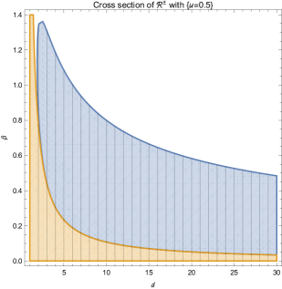
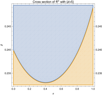
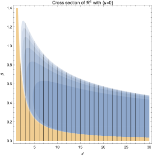
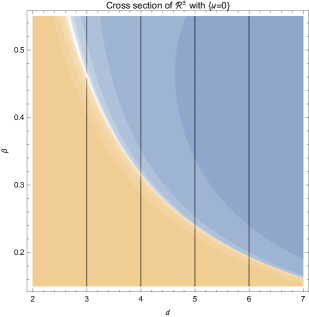
Figure 4: Regions $\mathcal{R}_{K}^{\pm}$ of parameters $(\beta,d,u)$ where we can guarantee that $\gamma_{T}$ is infinite with positive probability (blue region $\mathcal{R}^{+}_{K}$) and that $\gamma_{T}$ is finite almost surely (sandybrown region $\mathcal{R}^{-}_{K}$), respectively. On top, we considered $K=5$ while the bottom pictures show a comparison for $K=0,\ldots,5$ with regions of higher $K$ being more lightly coloured.

Before addressing the proof, let us look at an immediate consequence. If we combine the estimates of Lemma 4.1(a) and (b) with Proposition 3.2 and Lemma 3.3, we see that with positive probability there are infinite loops for all parameters within the region

$$\mathcal{R}^{+}_{K} :=\{(\beta,d,u)\in(0,\infty)\times\mathbb{N}\times[0,1]:\mathop{F_{K}}(\beta d,d^{-1},u)>1\},$$ (4.2)

while $$\gamma_{T}$$ is finite almost surely for

$$\begin{split}\mathcal{R}^{-}_{K}&:=\Big{\{}(\beta,d,u)\in(0,\infty)\times\mathbb{N}\times[0,1]:d(1-\mathrm{e}^{-\beta}(1+\beta))<1\\ &\qquad\qquad\text{ and }\frac{{\beta}d\mathrm{e}^{-{\beta}}}{1-{d}(1-\mathrm{e}^{-{\beta}}(1+{\beta}))}-\mathop{\bar{F}_{K}}({\beta}{d},d^{-1},{u})\leq 1\Big{\}}.\end{split}$$ (4.3)

Various cross sections of $\mathcal{R}^{\pm}_{K}$ are shown in Figure 2 and Figure 4, with the latter figure also containing a comparison of the precision of $\mathcal{R}^{\pm}_{K}$ for $K=0,\ldots,5$.

Proof of Lemma 4.1.

The estimate within (a) follows directly from (4.1) and the definition of $\mathop{F_{K}}$. Moreover, as

$$p_{S,n}(d,u)\leq p_{S,n}(d,u)+{\bar{p}}_{S,n}(d,u)=\frac{1}{n!}(d|V(S)|-|E(S)|)$$ (4.4)

we find

$$\begin{split}\mathbb{E}(|M_{1}|)\leq&-\mathop{\bar{F}_{K}}(\beta d,d^{-1},u)\\ &+\sum_{(S,n)\in\mathcal{S}_{d}}\left(\mathrm{e}^{-\beta d}(1+\beta)^{d-1}\right)^{|V(S)|}\beta^{n(S)+1}\frac{d|V(S)|-|E(S)|}{n!},\end{split}$$

$$= -\mathop{\bar{F}_{K}}(\beta d,d^{-1},u)+\sum_{(S,n)\in\mathcal{S}_{d}}\mathbb{P}(A_{S,n})\;\;\sum_{\mathclap{y\in V(S^{+})\setminus V(S)}}\;\;\mathbb{P}\left(N^{e_{y}^{-}}=1\,\big{|}\,A_{S,n}\right),$$

where the last equality follows from the proof of Lemma 3.4. Now, the sum on the right hand side is easily seen to be the expectation of the random variable $|W_{1}|$ with

$$W_{1}:=\{x\in V(C_{r}^{+})\setminus V(C_{r}):N^{e_{x}^{-}}=1\}.$$

Fortunately, for $d(1-\mathrm{e}^{-\beta}(1+\beta))<1$, this expectation can also be calculated in a more straightforward way. By applying Wald’s identity multiple times, we find

$$\mathbb{E}(|\{y\in V(C_{r}):|y|=n\}|) =\big{(}d(1-\mathrm{e}^{-\beta}(1+\beta))\big{)}^{n}$$

and thus

$$\mathbb{E}(|W_{1}|) =\sum_{n=1}^{\infty}\mathbb{E}(|\{x\in W_{1}:|x|=n\}|)$$

$$=\sum_{n=1}^{\infty}d\beta\mathrm{e}^{-\beta}\mathbb{E}(|\{y\in V(C_{r}):|y|=n-1\}|)$$

$$=\frac{\beta d\mathrm{e}^{-\beta}}{1-d(1-\mathrm{e}^{-\beta}(1+\beta))}.$$

For (c), let $0<\alpha\leq\hat{\alpha}$ and $d_{0}\leq d\in\mathbb{N}$ be given. We now use that

$$\begin{split}\mathbb{E}_{\beta=\alpha/d}(|M_{1}|)=&F_{K}(\alpha,d^{-1},u)\\ &+\sum_{\begin{subarray}{c}(S,n)\in\mathcal{S}_{d}:\\ \mathop{\operatorname{ord}}(S,n)>K\end{subarray}}\left(\mathrm{e}^{-\alpha}\left(1+\frac{\alpha}{d}\right)^{d-1}\right)^{|V(S)|}\left(\frac{\alpha}{d}\right)^{n(S)+1}p_{S,d}(d,u)\end{split}$$

and estimate the sum on the right hand side. By (4.4) and the facts that $|E(S)|\leq\mathop{\operatorname{ord}}(S,n)$ and $|E(S)|\geq 1$ for $\mathop{\operatorname{ord}}(S,n)\geq 1$, we find

$$\begin{split}&\mathbb{E}_{\beta=\alpha/d}(|M_{1}|)-F_{K}(\alpha,d^{-1},u)\\ &\leq\sum_{k=K+1}^{\infty}\sum_{\ell=1}^{k}\sum_{\begin{subarray}{c}S\subseteq T\text{ subtree}\\ \text{with root }r\\ \text{and }|E(S)|=\ell\end{subarray}}\sum_{\begin{subarray}{c}n\in(\mathbb{N}_{\geq 2})^{E(S)}:\\ n(S)=k+\ell\end{subarray}}{\underbrace{\left(\mathrm{e}^{-\alpha}\left(1+\frac{\alpha}{d}\right)^{d-1}\right)}_{\leq 1}}^{|V(S)|}\\ &\hphantom{\leq\sum_{k=K+1}^{\infty}\sum_{\ell=1}^{k}\sum_{\begin{subarray}{c}S\subseteq T\text{ subtree}\\ \text{with root }r\\ \text{and }|E(S)|=\ell\end{subarray}}\sum_{\begin{subarray}{c}n\in(\mathbb{N}_{\geq 2})^{E(S)}:\\ n(S)=k+\ell\end{subarray}}{\underbrace{\left(\mathrm{e}^{-\alpha}\left(1+\frac{\alpha}{d}\right)^{d-1}\right)}_{\leq 1}}^{|V(S)|}}\mathllap{\left(\frac{\alpha}{d}\right)^{n(S)+1}\frac{d|V(S)|-|E(S)|}{n!}}.\end{split}$$ (4.5)

Note that, within the last expression, we may write $n(S)$, $|V(S)|$ and $|E(S)|$ in terms of $k$ and $\ell$ instead of $S$. Moreover, by [19, Exercise 2.3.4.4-11 on p.397 and p.589], the number of subtrees $S\subseteq T$ of the $d$-ary tree $T$ with $r\in V(S)$ and $|V(S)|=\ell+1$ is given by the $(\ell+1)^{\text{th}}$ $d$-Fuss-Catalan number $\frac{1}{d(\ell+1)-\ell}{{d(\ell+1)}\choose{\ell+1}}$. Thus, by expanding the last summation within (4.5) onto all $n\in(\mathbb{N}_{0})^{E(S)}$ with $n(S)=k+\ell$, using the multinomial theorem and estimating ${{d(\ell+1)}\choose{\ell+1}}$ due to ${m\choose j}\leq m^{j}/j!$, we obtain

$$\begin{split}&\mathbb{E}_{\beta=\alpha/d}(|M_{1}|)-F_{K}(\alpha,d^{-1},u)\\ &\leq\sum_{k=K+1}^{\infty}\sum_{\ell=1}^{k}\frac{(\ell+1)^{\ell+1}}{(\ell+1)!}\frac{\alpha^{k+\ell+1}}{d^{k}}\frac{\ell^{k+\ell}}{(k+\ell)!}\end{split}$$

$$\leq\,\frac{1}{d^{K+1}}\underbrace{{\hat{\alpha}}^{K+3}\sum_{k=0}^{\infty}\left(\frac{\hat{\alpha}}{d_{0}}\right)^{k}\sum_{\ell=0}^{k+K}{\hat{\alpha}}^{\ell}\frac{(\ell+2)^{\ell+2}}{(\ell+2)!}\frac{(\ell+1)^{\ell+1}}{(\ell+1)!}\prod_{j=1}^{k+K+1}\frac{\ell+1}{\ell+1+j}}_{=:c_{K}}.$$

Now, by Stirling’s approximation $\frac{\ell^{\ell}}{\ell!}\leq\frac{\mathrm{e}^{\ell}}{\mathchoice{{\hbox{$\displaystyle\sqrt{2\pi\ell\,}$}\lower 0.4pt\hbox{\vrule height=4.8611pt,depth=-3.8889pt}}}{{\hbox{$\textstyle\sqrt{2\pi\ell\,}$}\lower 0.4pt\hbox{\vrule height=4.8611pt,depth=-3.8889pt}}}{{\hbox{$\scriptstyle\sqrt{2\pi\ell\,}$}\lower 0.4pt\hbox{\vrule height=3.40277pt,depth=-2.72223pt}}}{{\hbox{$\scriptscriptstyle\sqrt{2\pi\ell\,}$}\lower 0.4pt\hbox{\vrule height=2.43054pt,depth=-1.94444pt}}}}\leq\mathrm{e}^{\ell}$ we find

$$c_{K} \leq\hat{\alpha}^{K+3}\sum_{k=0}^{\infty}\left(\frac{\hat{\alpha}}{d_{0}}\right)^{k}\sum_{\ell=0}^{k+K}\hat{\alpha}^{\ell}\mathrm{e}^{2\ell+3}\prod_{j=1}^{k+K+1}\underbrace{\frac{\ell+1}{\ell+1+j}}_{\leq 1}$$

$$\leq\hat{\alpha}^{K+3}\mathrm{e}^{3}\sum_{k=0}^{\infty}\left(\frac{\hat{\alpha}}{d_{0}}\right)^{k}\frac{(\hat{\alpha}\mathrm{e}^{2})^{k+K+1}-1}{\hat{\alpha}\mathrm{e}^{2}-1}$$

$$\leq\left(\hat{\alpha}^{2}\mathrm{e}^{2}\right)^{K+1}\underbrace{\frac{\hat{\alpha}^{2}\mathrm{e}^{3}}{\hat{\alpha}\mathrm{e}^{2}-1}\sum_{k=0}^{\infty}\left(\frac{\hat{\alpha}^{2}\mathrm{e}^{2}}{d_{0}}\right)^{k}}_{=:c<\infty}$$

since we assumed that $\hat{\alpha}\mathrm{e}^{2}>1$ and $d_{0}>\hat{\alpha}^{2}\mathrm{e}^{2}$. ∎

Remark 4.2.

The proof of Lemma 4.1(a) and (b) shows that the given estimates correspond to estimating $\mathbb{E}(|M_{1}^{-}|)\leq\mathbb{E}(|M_{1}|)\leq\mathbb{E}(|M_{1}^{+}|)$, where $M_{1}^{\pm}$ are worst-case bounds on $M_{1}$ outside of $A_{K}:=\bigcup_{(S,n)\in\mathcal{S}_{d}:\mathop{\operatorname{ord}}(S,n)\leq K}A_{S,n}$. More precisely, we may define $M_{1}^{\pm}$ to coincide with $M_{1}$ on $A_{K}$ (i.e., on the set where we trace the propagation of $\gamma_{T}$ precisely), while we set $M_{1}^{-}:=\emptyset$ and $M_{1}^{+}:=W_{1}$ otherwise. This idea of tracing $\gamma_{T}$ whenever possible/viable and using worst-case estimates otherwise might be a practicable way to proceed in another context, too, even if there is no “perfect” sequence $(M_{n})_{n}$: If one is able to construct worst-case bounds $(M_{n}^{\pm})$ for the propagation of $\gamma_{T}$ by a construction similar to the one for $M_{1}$, this at least yields the sufficient conditions for both phases that correspond to the estimates from Lemma 4.1(a) and (b).

Apart from providing implicit but sharp phase-conditions for the parameters $(\beta,d,u)$, the estimates from Lemma 4.1 also allow us to find the asymptotic expansion of $\beta_{c}$.

Proof of Theorem 2.2.

Fix $u\in[0,1]$. Since the terms within $\mathop{F_{K}}(\alpha,h,u)$ contain the factor $h^{\mathop{\operatorname{ord}}(S,n)}$ and the only pair $(S,n)$ with $\mathop{\operatorname{ord}}(S,n)=0$ is $(S_{0},n_{0})$, with Example 3.5 and $\kappa_{S_{0},n_{0}}(d)=1$ we find

$$\mathop{F_{K}}(1,0,u)=1$$

as well as

$$\partial_{\alpha}\mathop{F_{K}}(\alpha,h,u)\big{|}_{\alpha=1,h=0} =1$$

for all $K\in\mathbb{N}_{0}$. Therefore, by the implicit function theorem for analytic functions (see Proposition A.1) there exist analytic functions $\alpha^{(K,\pm)}$ on a common neighbourhood of $h=0$ and such that

$$\mathop{F_{K}}(\alpha^{(K,+)}(h),h,u) =1$$

and

$$\mathop{F_{K}}(\alpha^{(K,-)}(h),h,u)+c_{K}h^{K+1} =1$$

for sufficiently small $|h|$, where $c_{K}$ is chosen according to Lemma 4.1(c) and $\hat{\alpha}:=2$. Moreover, by a corollary of the multivariate Faà Di Bruno formula (see Proposition A.1) the coefficients of $\alpha^{(K,\pm)}$ can be determined recursively by $\alpha_{0}=1$ and

$$\begin{split}\alpha_{k}=&\,\alpha_{k}(u)\\ :=&\,-\sum_{\begin{subarray}{c}j_{0},\ldots,j_{k-1}\in\mathbb{N}_{0}:\\ 1\leq\sum_{i=0}^{k-1}j_{i}\leq k,\\ j_{0}+\sum_{i=1}^{k-1}ij_{i}=k\end{subarray}}\frac{\partial_{h}^{j_{0}}\partial_{\alpha}^{j_{1}+\ldots+j_{k-1}}F_{k}(\alpha,h,u)\big{|}_{\alpha=1,h=0}}{\prod_{i=0}^{k-1}j_{i}!}\prod_{i=1}^{k-1}\alpha_{i}^{j_{i}},\end{split}$$ (4.6)

$k=1,\ldots,K$. Here, we used that

$$\partial_{h}^{j}F_{k}(\alpha,h,u)\big{|}_{h=0} =\partial_{h}^{j}\mathop{F_{K}}(\alpha,h,u)\big{|}_{h=0}$$

$$=\partial_{h}^{j}\left(\mathop{F_{K}}(\alpha,h,u)+c_{K}h^{K+1}\right)|_{h=0}$$

for $j\leq k\leq K$ since these functions differ by terms containing the factor $h^{j+1}$. In particular, for $0\leq k\leq K$, the $k^{\text{th}}$ coefficients of $\alpha^{(K,+)}$ and $\alpha^{(K,-)}$ coincide with $\alpha_{k}$ and they do not depend on the choice of $K$. This yields

$$\alpha^{(K,\pm)}(h)=\sum_{k=0}^{K}\alpha_{k}h^{k}+\mathcal{O}(h^{K+1})$$ (4.7)

as $h\to 0$ with the $\mathcal{O}$-term of course differing for $\alpha^{(K,+)}$ and $\alpha^{(K,-)}$. Furthermore, by an easy induction argument the recursion (4.6) yields that every $\alpha_{k}(u)$ is a polynomial in $u$ as $F_{k}$ is a polynomial in $u$. Finally, by Lemma 4.1(a), for $\beta^{+}=d^{-1}\,\alpha^{(K,+)}(d^{-1})$ we find that

$$\mathbb{E}_{\beta^{+}}(|M_{1}|)\geq\mathop{F_{K}}(\alpha^{(K,+)}(d^{-1}),d^{-1},u)=1=\mathbb{E}_{\beta_{c}}(|M_{1}|)$$

for all sufficiently large $d$. Thus, by monotonicity (see Proposition 3.6) we find that

$$\beta_{c}\leq\beta^{+}=d^{-1}\,\alpha^{(K,+)}(d^{-1})$$

for those $d$. Similarly, from Lemma 4.1(c), we obtain

$$\beta_{c}\geq d^{-1}\,\alpha^{(K,-)}(d^{-1})$$

for large $d$. Combined with (4.7), this completes the proof. ∎

5 Reduction to a combinatorial problem

In this section, we are going to present a method to calculate the polynomials $p_{S,n}$ and $\bar{p}_{S,n}$, respectively, for every fixed $[(S,n)]\in\mathcal{S}$ with $E(S)\neq\emptyset$. For this purpose, it suffices to calculate $\mathbb{E}\left(\frac{\tau_{S}^{x}}{\beta}\big{|}A_{S,n}\right)$ for all $x\in V(S)$ (compare with the discussion in the beginning of Section 4) and we will determine this quantity by partitioning $A_{S,n}$ into the events $A_{S,n,\nu}$ where the cluster $C_{r}$ is fixed to coincide with $S$ and the total number $N^{e}$ of links on every edge $e\in E(S)$ is given by $n(e)$, i.e.,

$$\begin{split}A_{S,n,\nu}:=&A_{S,n}\cap\{\text{For all }j=1,\ldots,n(S)\text{ the }j^{\text{th}}\text{ link}\text{ on }S\\ &\hphantom{A_{S,n}\cap\{}\text{is of type }\star_{j}\text{ and occurs on the edge }e_{j}\},\end{split}$$

where

$$\nu= ((e_{1},\star_{1}),\ldots,(e_{n(S)},\star_{n(S)}))\in\mathcal{V}_{S,n},$$

$$\mathcal{V}_{S,n}:= \big{\{}((\epsilon_{j},*_{j}))_{j=1}^{n(S)}:|\{j:\epsilon_{j}=e\}|=n(e)\text{ for all }e\in E(S)\big{\}}.$$

Moreover, the time-ordering of the edges and types of the links is specified by the sequence $\nu$. Here, time-ordering is understood via $\mathop{\mathbb{T}_{\beta}}\simeq[0,\beta)$ and in particular, the $j^{\text{th}}$ link is determined with respect to this order. Given $A_{S,n,\nu}$, determining the loop configuration is then closely related to the following task.

Combinatorial Problem 5.1.

Fix $[(S,n)]\in\mathcal{S}$ with $E(S)\neq\emptyset$ and $\nu=((e_{j},\star_{j}))_{j=1}^{n(S)}\in\mathcal{V}_{S,n}$. Now, for $j=1,\ldots,n(S)$, place a link of type $\star_{j}$ onto the edge $e_{j}$ at position $\tfrac{j}{n(S)+1}\beta$, i.e. consider the deterministic link configuration $X_{\nu}=(X_{\nu}^{e,\star})_{e\in E(S),\star\in\{\mathop{\backslash\mathllap{/}},\mathop{||}\}}$ with

$$X_{\nu}^{e,\star}=\;\;\sum_{\mathclap{\begin{subarray}{c}j=1,\ldots,n(S):\\ e_{j}=e\text{ and }\star_{j}=\star\end{subarray}}}\;\;\delta_{\frac{j}{n(S)+1}\beta}.$$ (5.1)

For this configuration, consider the loop $\gamma_{S}(X_{\nu})$ on the tree $S$ that contains $(r,0)$ and compute the combinatorial quantities

$$b_{S,\nu}^{x}:=\left|\left\{j\in\{0,\ldots,n(S)\}:\{x\}\times\left(\tfrac{j}{n(S)+1}\beta,\tfrac{j+1}{n(S)+1}\beta\right)\subseteq\gamma_{S}(X_{\nu})\right\}\right|$$ (5.2)

for all $x\in V(S)$.

Figure 5: Let $S_{1}$ be the tree containing two vertices and one edge $e_{1}=\{r,x_{1}\}$ between them. Furthermore, let $n_{1}(S_{1})=n_{1}(e_{1}):=2$ be the number of links on this edge and define their types by $\nu:=((e_{1},\mathop{\backslash\mathllap{/}}),(e_{1},\mathop{\backslash\mathllap{/}}))$. Then the link configuration $X_{\nu}$ on $E(S)$ and its corresponding loop configuration are depicted above. For every vertex $x\in V(S_{1})$, one can now easily read off the number $b^{x}_{S_{1},\nu}$ of intervals $\left(\tfrac{j}{n(S)+1}\beta,\tfrac{j+1}{n(S)+1}\beta\right)$ that the (blue) loop $\gamma_{S_{1}}(X_{\nu})$ stays at this vertex.

Remark 5.2.

One can solve the task of Combinatorial Problem 5.1 (i.e., determine the integers $b_{S,\nu}^{x}$ for all $x\in V(S)$) with the help of a computer or by drawing a sketch (see Figure 5 and the description within its caption). Unfortunately, this will take more and more computational effort as $n(S)$ and $|E(S)|$ increase. However, note that at least the calculation of $b_{S,\nu}^{x}$ does not depend on the choice of the representative for $[(S,n)]$ if $\nu$ is adapted accordingly.

The connection between Combinatorial Problem 5.1 and the calculation of $p_{S,n}$ and $\bar{p}_{S,n}$ is established by the following lemma.

Lemma 5.3.

For all $(S,n)\in\mathcal{S}_{d}$ with $E(S)\neq\emptyset$ and $\nu\in\mathcal{V}_{S,n}$ we have

$$\mathbb{E}\left(\frac{\tau_{S}^{x}}{\beta}\,\bigg{|}\,A_{S,n,\nu}\right)=\frac{b_{S,\nu}^{x}}{n(S)+1},$$

with $b_{S,\nu}^{x}$ given by (5.2). In particular,

$$p_{S,n}(d,u)= \,\frac{1}{(n(S)+1)!}\sum_{\nu\in\mathcal{V}_{S,n}}u^{\nu}\sum_{x\in V(S)}(d-d_{S}^{x})b_{S,\nu}^{x}$$ (5.3)

and

$$\bar{p}_{S,n}(d,u)= \,\frac{1}{(n(S)+1)!}\sum_{\nu\in\mathcal{V}_{S,n}}u^{\nu}\sum_{x\in V(S)}(d-d_{S}^{x})\bar{b}_{S,\nu}^{x},$$ (5.4)

where for $$\nu=((e_{j},\star_{j}))_{j=1}^{n(S)}$$ we set

$$u^{\nu}:= \,u^{|\{j:\star_{j}=\mathop{\backslash\mathllap{/}}\}|}(1-u)^{|\{j:\star_{j}=\mathop{||}\}|},$$

$$\bar{b}_{S,\nu}^{x}:= \,n(S)+1-b_{S,\nu}^{x}.$$

Proof.

To begin with, denote the positions of links on $E(S)$ by $t_{1}<\ldots<t_{n(S)}$ and set $t_{0}:=0$, $t_{{n(S)}+1}:=\beta$. Moreover, fix $x\in V(S)$ and let $b^{x,j}_{S,\nu}\in\{0,1\}$, $j=0,\ldots,n(S),$ be the indicator of $\{\gamma_{S}\text{ contains }\{x\}\times(t_{j},t_{j+1})\}$ when given $A_{S,n,\nu}$. Note that each $b^{x,j}_{S,\nu}$ is deterministic for given $S,\nu,x$ and $j$. In particular, a change of $(t_{1},\ldots,t_{n(S)})$ that preserves the time-ordering does not change the $b^{x,j}_{S,\nu}$’s. Therefore, we find $b^{x,j}_{S,\nu}=b^{x,j}_{S,\nu}(X_{\nu})$ with $X_{\nu}$ as in (5.1). This yields

$$\tau_{S}^{x}=\sum_{j=0}^{n(S)}b^{x,j}_{S,\nu}(X_{\nu})(t_{j+1}-t_{j})$$

on $A_{S,n,\nu}$. Now, with respect to the conditional measure $\mathbb{P}(\,\cdot\,\big{|}\,A_{S,n,\nu})$, the vector $(t_{1},\ldots,t_{n(S)})$ is uniformly distributed on $\{s\in\mathbb{R}^{n(S)}:0<s_{1}<\ldots<s_{n(S)}<\beta\}$ since it is the vector of arrival times of a merged Poisson process, where the number of jumps and the assignment of these jumps to the respective subprocesses is fixed by $A_{S,n,\nu}$. Therefore, we have

$$\mathbb{E}\left(\frac{\tau_{S}^{x}}{\beta}\,\bigg{|}\,A_{S,n,\nu}\right)=\sum_{j=0}^{n(S)}b_{S,\nu}^{x,j}(X_{\nu})\underbrace{\mathbb{E}\left(\frac{t_{j+1}-t_{j}}{\beta}\,\bigg{|}\,A_{S,n,\nu}\right)}_{=\frac{1}{n(S)+1}}=\frac{b_{S,\nu}^{x}}{n(S)+1}.$$

Finally, the assertions about $p_{S,n}$ and $\bar{p}_{S,n}$, respectively, follow if we decompose $A_{S,n}=\bigcup_{\nu\in\mathcal{V}_{S,n}}A_{S,n,\nu}$ and use that $\mathbb{P}(A_{S,n,\nu}\,\big{|}\,A_{S,n})=u^{\nu}\frac{n!}{n(S)!}$. ∎

Note that so far we excluded the case $[(S,n)]=[(S_{0},n_{0})]$ within the considerations in this section since the definition of $A_{S,n,\nu}$ would need clarification to make sense for $E(S)=\emptyset$. Nevertheless, Example 3.5 shows that (5.3) and (5.4) remain valid if we set $\nu=(\emptyset)$ to be the empty list and $\mathcal{V}_{S_{0},n_{0}}=\{\nu\}$ as well as $b^{r}_{S_{0},\nu}=1=u^{\nu}$.

Before we address the proof of Theorem 2.1 for $d=3,4$, let us present computational results for the integers $b_{S,\nu}^{x}$. For the sake of a concise arrangement, we define

$$\mathcal{V}_{S,n,j}:=\{((e_{i},\star_{i}))_{i=1}^{n(S)}\in\mathcal{V}_{S,n}:|\{i:\star_{i}=\mathop{||}\}|=j\},\qquad j=0,\ldots,n(S)$$

and set $D_{S,n}$ to be the $2\times(n(S)+1)$-matrix for which the $k^{\text{th}}$ column is given by

$$(D_{S,n})_{k}= \sum_{\nu\in\mathcal{V}_{S,n,k-1}}\sum_{x\in V({S})}\begin{pmatrix}b^{x}_{S,\nu}\\ d_{S}^{x}\,b^{x}_{S,\nu}\end{pmatrix},\qquad k=1,\ldots,n(S)+1.$$

Analogously, we define $\bar{D}_{S,n}$ but with $b^{x}_{S,\nu}$ replaced by $\bar{b}^{x}_{S,\nu}$. This yields

$$p_{S,n}(d,u)= \,\frac{1}{(n(S)+1)!}\left\langle D_{S,n}\mathbf{u}^{(n(S))},\begin{pmatrix}d\\ -1\end{pmatrix}\right\rangle$$

and the analogous equation for $\bar{p}_{S,n}$, where we set

$$\mathbf{u}^{(n(S))}:= \,\left(u^{n(S)},u^{n(S)-1}(1-u),\ldots,(1-u)^{n(S)}\right)^{\textsf{T}}\in[0,1]^{n(S)+1}.$$

Note that the entries of $D_{S,n}$ and $\bar{D}_{S,n}$ are integers and they do not depend on the specific choice for the representative of $[(S,n)]$, see Remark 5.2. To demonstrate how to compute their entries, let us look at an example.

Figure 6: The three sequences $\nu\in\mathcal{V}_{S_{3},n_{3},2}$, see Example 5.4 for a description.

Example 5.4.

Consider $S_{2}=(\{r,x_{1}\},\{e_{1}=\{r,x_{1}\}\})$ and $n_{2}(S_{2})=n_{2}(e_{1})=3$ as well as link configurations with $j=2$ links of type $\mathop{||}$. Then the set $\mathcal{V}_{S_{2},n_{2},2}$ consists of the three sequences $\nu$ listed on top of Figure 6. Similar to Figure 5, one can read off the numbers $b_{S_{2},\nu}^{x}$ with $x\in V(S_{2})$ and $\nu\in\mathcal{V}_{S_{2},n_{2},2}$ by constructing the (blue) loop $\gamma_{S_{2}}(X_{\nu})$ (see bottom line of Figure 6). Since $d_{S_{2}}^{r}=1$ and $d_{S_{2}}^{x_{1}}=0$, the third column of $D_{S_{2},n_{2}}$ becomes

$$(D_{S_{2},n_{2}})_{3}=\begin{pmatrix}3+3&+&2+2&+&3+3\\ 3+0&+&2+0&+&3+0\end{pmatrix}=\begin{pmatrix}16\\ 8\end{pmatrix}.$$

All other columns of $D_{S_{2},n_{2}}$ are determined analogously.

Sketch of	$\mathop{\operatorname{ord}}(S,n)$	$n(S)$	$|V({S})|$	$\kappa_{S,n}(d)$	computed results
$[(S,n)]$					$D_{S,n}$	$\bar{D}_{S,n}$
	$0$	$0$	$1$	$1$	$\displaystyle{\begin{pmatrix}1\\ 0\end{pmatrix}}$	$\displaystyle{\begin{pmatrix}0\\ 0\end{pmatrix}}$
	$1$	$2$	$2$	$d$	$\displaystyle{\begin{pmatrix}3&12&4\\ 2&6&2\end{pmatrix}}$	$\displaystyle{\begin{pmatrix}3&0&2\\ 1&0&1\end{pmatrix}}$
	$2$	$3$	$2$	$d$	$\displaystyle{\begin{pmatrix}8&24&16&4\\ 4&12&8&2\end{pmatrix}}$	$\displaystyle{\begin{pmatrix}0&0&8&4\\ 0&0&4&2\end{pmatrix}}$
	$2$	$4$	$3$	$\displaystyle{{d\choose 2}}$	$\displaystyle{\begin{pmatrix}50&260&414&292&60\\ 40&192&288&192&40\end{pmatrix}}$	$\displaystyle{\begin{pmatrix}40&100&126&68&30\\ 20&48&72&48&20\end{pmatrix}}$
	$2$	$4$	$3$	$d^{2}$	$\displaystyle{\begin{pmatrix}50&250&415&306&65\\ 39&190&287&206&44\end{pmatrix}}$	$\displaystyle{\begin{pmatrix}40&110&125&54&25\\ 21&50&73&34&16\end{pmatrix}}$
	$3$	$4$	$2$	$d$	$\displaystyle{\begin{pmatrix}5&40&40&20&4\\ 3&20&20&10&2\end{pmatrix}}$	$\displaystyle{\begin{pmatrix}5&0&20&20&6\\ 2&0&10&10&3\end{pmatrix}}$
	$3$	$5$	$3$	$d(d-1)$	$\displaystyle{\begin{pmatrix}102&750&1396&1348&624&104\\ 80&528&960&900&408&68\end{pmatrix}}$	$\displaystyle{\begin{pmatrix}78&150&404&452&276&76\\ 40&72&240&300&192&52\end{pmatrix}}$
	$3$	$5$	$3$	$d^{2}$	$\displaystyle{\begin{pmatrix}114&774&1418&1382&646&110\\ 92&560&982&932&426&72\end{pmatrix}}$	$\displaystyle{\begin{pmatrix}66&126&382&418&254&70\\ 28&40&218&268&174&48\end{pmatrix}}$
	$3$	$5$	$3$	$d^{2}$	$\displaystyle{\begin{pmatrix}84&696&1386&1430&710&126\\ 62&482&950&980&490&88\end{pmatrix}}$	$\displaystyle{\begin{pmatrix}96&204&414&370&190&54\\ 58&118&250&220&110&32\end{pmatrix}}$
	$3$	$6$	$4$	$d^{2}(d-1)$	$\displaystyle{\begin{pmatrix}1162&9268&25614&36910&28483&11254&1539\\ 1127&8186&21292&29264&21899&8534&1182\end{pmatrix}}$	$\displaystyle{\begin{pmatrix}1358&5852&12186&13490&9317&3866&981\\ 763&3154&7058&8536&6451&2806&708\end{pmatrix}}$
	$3$	$6$	$4$	$\displaystyle{d\cdot{d\choose 2}}$	$\displaystyle{\begin{pmatrix}1232&9996&25748&37964&28888&12320&1652\\ 1090&8388&20918&29840&22046&9228&1258\end{pmatrix}}$	$\displaystyle{\begin{pmatrix}1288&5124&12052&12436&8912&2800&868\\ 800&2952&7432&7960&6304&2112&632\end{pmatrix}}$
	$3$	$6$	$4$	$d^{3}$	$\displaystyle{\begin{pmatrix}1022&8456&24204&36386&28943&11634&1615\\ 923&7238&19986&28854&22248&8876&1245\end{pmatrix}}$	$\displaystyle{\begin{pmatrix}1498&6664&13596&14014&8857&3486&905\\ 967&4102&8364&8946&6102&2464&645\end{pmatrix}}$
	$3$	$6$	$4$	$\displaystyle{{d\choose 3}}$	$\displaystyle{\begin{pmatrix}1260&10332&26208&37764&27900&11592&1512\\ 1134&8568&21186&29376&21186&8568&1134\end{pmatrix}}$	$\displaystyle{\begin{pmatrix}1260&4788&11592&12636&9900&3528&1008\\ 756&2772&7164&8424&7164&2772&756\end{pmatrix}}$

Table 2: The considered prototypes of edge-weighted rooted trees $[(S,n)]\in\mathcal{S}$ are sorted by their order $\mathop{\operatorname{ord}}(S,n)$ and displayed together with algorithmically computed results $D_{S,n}$, $\bar{D}_{S,n}$. For each pair $[(S,n)]$, the values of $n(e)$ are attached to their corresponding edge $e$ and the root is always depicted as the bottom vertex.

Similar to Example 5.4, we have determined the matrices $D_{S,n}$ for all $[(S,n)]\in\mathcal{S}$ with $\mathop{\operatorname{ord}}(S,n)\leq 5$ and (for $\mathop{\operatorname{ord}}(S,n)\leq 3$) they are listed within Table 2. Together with the corresponding multiplicities $\kappa_{S,n}(d)$ that are also listed in this table, this allows us to calculate $\mathop{F_{K}}(\alpha,h,u)$ and $\mathop{\bar{F}_{K}}(\alpha,h,u)$ for $0\leq K\leq 5$ and all $(\alpha,h,u)$. In particular, we may now compute the coefficients $\alpha_{k}(u)$ using (4.6) and the results are given in Table 1. Furthermore, we may now complete the proof of Theorem 2.1.

Proof of Theorem 2.1 for $d=3,4$.

By Proposition 3.6, it is sufficient to show that $\mathbb{E}_{\beta=d^{-1/2}}(|M_{1}|)>1$. Moreover, by Lemma 4.1(a), a sufficient condition for the latter statement is $F_{5}(d^{-1/2}d,d^{-1},u)>1$ and one sees that this holds for $d=3,4$ (compare Figure 7). ∎

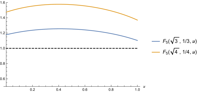
Figure 7: Plot of $F_{5}(d^{1/2},d^{-1},u)$ as a function of $u$ for $d=3,4$. In particular, both graphs are strictly above $1$ uniformly in $u$.

Remark 5.5 (Concerning a sharp phase transition for $d=2$).

In Theorem 2.1, the case $d=2$ of the binary tree is excluded. In this boundary case we are missing two crucial properties: On the one hand, we need to find a sufficiently large $\beta^{*}>0$ (possibly depending on $u$) such that we can show $\mathbb{E}_{\beta^{*}}(|M_{1}|)>1$ for all $u$ by an appropriate estimate. On the other hand, $\beta^{*}$ needs to be small enough that $(0,\beta^{*}]\ni\beta\mapsto\mathbb{E}_{\beta}(|M_{1}|)$ is strictly increasing.
Note that, for $d=2$, we would need to choose $\beta^{*}>d^{-1/2}$ since a numerical evaluation of $\bar{F}_{5}$ yields $\mathbb{E}_{\beta=d^{-1/2}}(|M_{1}|)\leq 1$ for $d=2$ and all $u$. Unfortunately, this means that our proof of monotonicity (see Proposition 3.6) fails as $f_{S_{0},n_{0}}(\beta)$ is decreasing for $\beta>d^{-1/2}$ and thus, the representation of $\mathbb{E}(|M_{1}|)$ given in Lemma 3.4 becomes a sum where some terms are increasing and some are decreasing.
Nevertheless, up to $\beta^{*}=1$ and for all $[(S,n)]\in\mathcal{S}$ excluding $[(S_{0},n_{0})]$, the map $\beta\mapsto f_{S,n}(\beta)$ remains strictly increasing and numerical results suggest that $\mathbb{E}_{\beta}(|M_{1}|)$ remains increasing up to this value, too. Moreover, for $d=2$ and $\mathop{\beta^{*}}=1$, we find that $F_{5}(\mathop{\beta^{*}}d,d^{-1},u)>1$ holds for a large range of $u$ including $u=\tfrac{1}{2}$. For the missing values of $u$ (in particular for $u=0,1$) an approximation by $\mathop{F_{K}}$ with $K=9$ should suffice to show that there also is a phase of infinite loops.

Appendix A Analytic equations and their solutions

Suppose that we are given an equation $f(x,y)=0$ and some $x_{0},y_{0}\in\mathbb{R}$ with $f(x_{0},y_{0})=0$. Then the classical implicit function theorem gives a sufficient condition such that one may find a unique solution $y=g(x)$ to this equation in a neighbourhood of $x_{0}$. If the function $f$ is in fact analytic, then $g$ can be shown to be analytic, too. Moreover, there exists an explicit recursion (involving the derivatives of $f$) to determine the coefficients of the series expansion of $g$ around $x_{0}$.

Proposition A.1.

Let $f\colon U\to\mathbb{R}$ be an analytic function in a neighbourhood $U\subseteq\mathbb{R}^{2}$ of $(x_{0},y_{0})\in U$. If $f(x_{0},y_{0})=0$ and $D_{2}f(x_{0},y_{0})\neq 0$, then there exists a neighbourhood $V$ of $x_{0}$ and an analytic function $g\colon V\to\mathbb{R},\,g(x)=\sum_{i=0}^{\infty}a_{i}(x-x_{0})^{i}$ with $f(x,g(x))=0$ for all $x\in V$. Moreover, $a_{0}=y_{0}$ and for $k=1,2,\ldots$ we have

$$a_{k}=-\sum\frac{(D_{1}^{j_{0}}D_{2}^{j_{1}+\ldots+j_{k-1}}f)(x_{0},a_{0})}{(D_{2}f)(x_{0},a_{0})\,\prod_{i=0}^{k-1}j_{i}!}\prod_{i=1}^{k-1}a_{i}^{j_{i}},$$

where the sum runs over all $j_{0},\ldots,j_{k-1}\in\mathbb{N}_{0}$ such that

$$1\leq\sum_{i=0}^{k-1}j_{i}\leq k\quad\text{and}\quad j_{0}+\sum_{i=1}^{k-1}ij_{i}=k.$$

Proof.

By the implicit function theorem for analytic functions (see e.g. [20, Theorem 2.3.1]), there exists an analytic function $g$ in some neighbourhood $V$ of $x_{0}$ with $a_{0}=g(x_{0})=y_{0}$ and $f(x,g(x))=0$ for all $x\in V$. Thus, on the one hand, we have

$$\frac{1}{k!}\frac{\mathrm{d}^{k}}{\mathrm{d}x^{k}}f(x,g(x))\big{|}_{x=x_{0}}=\frac{1}{k!}\frac{\mathrm{d}^{k}}{\mathrm{d}x^{k}}0\big{|}_{x=x_{0}}=0$$ (A.1)

for all $k\in\mathbb{N}$. On the other hand, the multivariate version of Faà di Bruno’s formula (see e.g. [14, Cor 2.11]) yields

$$\begin{split}\frac{1}{k!}\frac{\mathrm{d}^{k}}{\mathrm{d}x^{k}}f(x,g(x))\big{|}_{x=x_{0}}&=\sum_{\begin{subarray}{c}\lambda,\mu\in\mathbb{N}_{0}:\\ 1\leq\lambda+\mu\leq k\end{subarray}}\sum_{p(k,\lambda,\mu)}D_{1}^{\lambda}D_{2}^{\mu}f(x_{0},g(x_{0}))\\ &\qquad\qquad\prod_{i=1}^{k}\frac{\left(\operatorname{id}^{(i)}(x_{0})\right)^{\ell_{i}}\left(g^{(i)}(x_{0})\right)^{j_{i}}}{\ell_{i}!j_{i}!(i!)^{\ell_{i}+j_{i}}},\end{split}$$ (A.2)

where

$$\begin{split}p(k,\lambda,\mu)&=\{\ell_{1},\ldots,\ell_{k},j_{1},\ldots,j_{k}\geq 0:\\ &\qquad\sum_{i=1}^{k}\ell_{i}=\lambda,\sum_{i=1}^{k}j_{i}=\mu,\sum_{i=1}^{k}i(\ell_{i}+j_{i})=k\}.\end{split}$$

Since $\operatorname{id}^{(i)}(0)=0$ for all $i\geq 2$, the summands in (A.2) with $\ell_{i}>0$ for some $i\geq 2$ vanish. For all other summands we have $\ell_{2}=\ldots=\ell_{k}=0,\ell_{1}=\lambda-\sum_{i=2}^{k}\ell_{i}=\lambda$ and $k=\sum_{i=1}^{k}i(\ell_{i}+j_{i})=\lambda+\sum_{i=1}^{k}ij_{i}$. We now use that $g(x_{0})=a_{0}$ and $g^{(i)}(x_{0})=i!\,a_{i}$ to obtain

$$\begin{split}\frac{1}{k!}\frac{\mathrm{d}^{k}}{\mathrm{d}x^{k}}f(x,g(x))\big{|}_{x=x_{0}}=&\sum_{\begin{subarray}{c}\lambda,\mu\in\mathbb{N}_{0}:\\ 1\leq\lambda+\mu\leq k\end{subarray}}\sum_{\begin{subarray}{c}j_{1},\ldots,j_{k}\geq 0:\\ \sum_{i=1}^{k}j_{i}=\mu,\\ \lambda+\sum_{i=1}^{k}ij_{i}=k\end{subarray}}D_{1}^{\lambda}D_{2}^{\mu}f(x_{0},a_{0})\;\frac{1}{\lambda!}\prod_{i=1}^{k}\frac{a_{i}^{j_{i}}}{j_{i}!}.\end{split}$$

Let us investigate those summands within the right hand side of this equation with $j_{k}\geq 1$. Then $k\geq k-\lambda=\sum_{i=1}^{k}ij_{i}\geq kj_{k}\geq k$. In particular, all these inequalities are equalities, actually. Therefore, $j_{k}\geq 1$ implies

$$\lambda=0=j_{1},\ldots,j_{k-1}\quad\text{and}\quad\mu=j_{k}=1.$$

Thus, there is only one summand with $j_{k}\neq 0$, namely the one with these parameters and it is given by $D_{2}f(x_{0},a_{0})\,a_{k}$. For all other summands we have $j_{k}=0$ and, in particular, $\frac{a_{k}^{j_{k}}}{j_{k}!}=1$. Moreover, these other summands fulfill $\mu=\sum_{i=1}^{k-1}j_{i}$. Thus, by writing $j_{0}:=\lambda$ we find

$$\begin{split}\frac{1}{k!}\frac{\mathrm{d}^{k}}{\mathrm{d}x^{k}}f(x,g(x))\big{|}_{x=x_{0}}=&D_{2}f(x_{0},a_{0})\,a_{k}\\ +&\sum_{\begin{subarray}{c}j_{0},\ldots,j_{k-1}\geq 0:\\ 1\leq j_{0}+\sum_{i=1}^{k-1}j_{i}\leq k,\\ j_{0}+\sum_{i=1}^{k-1}ij_{i}=k\end{subarray}}\frac{(D_{1}^{j_{0}}D_{2}^{j_{1}+\ldots+j_{k-1}}f)(x_{0},a_{0})}{\prod_{i=0}^{k-1}j_{i}!}\prod_{i=1}^{k-1}a_{i}^{j_{i}}.\end{split}$$

Together with (A.1), this yields the assertion. ∎

References

- [1] Radosław Adamczak, Michał Kotowski, and Piotr Miłoś. Phase transition for the interchange and quantum Heisenberg models on the Hamming graph. 2018. arXiv:1808.08902.
- [2] Michael Aizenman and Bruno Nachtergaele. Geometric aspects of quantum spin states. Communications in Mathematical Physics, 164(1):17–63, 1994.
- [3] Omer Angel. Random infinite permutations and the cyclic time random walk. Discrete Mathematics and Theoretical Computer Science, AC:9–16, 2003.
- [4] K.B. Athreya and P.E. Ney. Branching Processes. Springer, 1972.
- [5] Alessandro Barp, Edoardo Gabriele Barp, François-Xavier Briol, and Daniel Ueltschi. A numerical study of the 3D random interchange and random loop models. Journal of Physics A: Mathematical and Theoretical, 48(34):345002, 2015.
- [6] Nathanaël Berestycki. Emergence of giant cycles and slowdown transition in random transpositions and -cycles. Electronic Journal of Probability, 16:152–173, 2011.
- [7] Nathanaël Berestycki and Gady Kozma. Cycle structure of the interchange process and representation theory. Bulletin de la Société Mathématique de France, 143(2), 2015.
- [8] Volker Betz, Johannes Ehlert, and Benjamin Lees. Phase transition for loop representations of quantum spin systems on trees. Journal of Mathematical Physics, 59(11):113302, 2018.
- [9] Jakob Björnberg. Large cycles in random permutations related to the heisenberg model. Electronic Communications in Probability, 20:1–11, 2015.
- [10] Jakob Björnberg, Michał Kotowski, Benjamin Lees, and Piotr Miłoś. The interchange process with reversals on the comlete graph. Electronic Journal of Probability, 24(108):1–43, 2019.
- [11] Jakob Björnberg and Daniel Ueltschi. Critical parameter of random loop model on trees. Annals of Applied Probability, 28:2063–2082, 2018.
- [12] Jakob Björnberg and Daniel Ueltschi. Critical Temperature of Heisenberg Models on Regular Trees, via Random Loops. Journal of Statistical Physics, 173(5):1369–1385, 2018.
- [13] Jakob E. Björnberg, Jürg Fröhlich, and Daniel Ueltschi. Quantum spins and random loops on the complete graph. 2018. arXiv:1811.12834.
- [14] G. M. Constantine and T. H. Savits. A multivariate Faa di Bruno formula with applications. Transactions of the American Mathematical Society, 348(2):503–520, 1996.
- [15] Alan Hammond. Infinite cycles in the random stirring model on trees. Bulletin of the Institute of Mathematics Academia Sinica, 8(4):85–104, 2013.
- [16] Alan Hammond. Sharp phase transition in the random stirring model on trees. Probability Theory and Related Fields, 161(3):429–448, 2015.
- [17] Alan Hammond and Milind Hegde. Critical point for infinite cycles in a random loop model on trees. The Annals of Applied Probability, 29(4):2067–2088, 2019.
- [18] T.E. Harris. Nearest-neighbor Markov interaction processes on multidimensional lattices. Advances in Mathematics, 9(1):66–89, 1972.
- [19] Donald E. Knuth. The Art of Computer Programming, Vol. 1: Fundamental algorithms. Addison-Wesley, 3rd edition, 1997.
- [20] Steven G. Krantz and Harold R. Parks. A Primer of Real Analytic Functions. Birkhäuser, 2nd edition, 2002.
- [21] Piotr Miłoś and Batı Şengül. Existence of a phase transition of the interchange process on the Hamming graph. Electronic Journal of Probability, 24(64):1–21, 2019.
- [22] Peter Mühlbacher. Critical parameters for loop and Bernoulli percolation. 2019. arXiv:1908.10213.
- [23] Oded Schramm. Compositions of random transpositions. Israel Journal of Mathematics, 147(1):221–243, 2005.
- [24] Bálint Tóth. Improved lower bound on the thermodynamic pressure of the spin 1/2 Heisenberg ferromagnet. Letters in Mathematical Physics, 28(1):75–84, 1993.
- [25] Daniel Ueltschi. Random loop representations for quantum spin systems. Journal of Mathematical Physics, 54(8):083301, 2013.