Dressed Quantum Trajectories: Novel Approach to the non-Markovian Dynamics of Open Quantum Systems on a Wide Time Scale

Abstract

A new approach to the theory and simulation of the non-Markovian dynamics of open quantum systems is presented. It is based on identification of a parameter which is uniformly small on wide time intervals: the occupation of the virtual cloud of quanta. By “virtual” we denote those bath excitations which were emitted by the system, but eventually will be reabsorbed before any measurement of the bath state. A favourable property of the virtual cloud is that the number of its quanta is expected to saturate on long times, since physically this cloud is a (retarded) polarization of the bath around the system. Therefore, the joint state of open system and of virtual cloud (the dressed state) can be accurately represented in a truncated basis of Fock states, on a wide time scale. At the same time, there can be arbitrarily large number of observable quanta, especially if the open system is under driving. However, by employing a Monte Carlo sampling of the measurement outcomes of the bath, we can simulate the dynamics of the observable quantum field. In this work we consider the measurement with respect to the coherent states, which yields the Husimi function as the positive (quasi)probability distribution of the outcomes. The evolution of dressed state which corresponds to a particular fixed outcome is called the dressed quantum trajectory. Therefore, the Monte Carlo sampling of these trajectories yields a stochastic simulation method with promising convergence properties on wide time scales.

I INTRODUCTION

The model of a finite quantum system coupled to an inifinite harmonic bath (the open quantum system, abbreviated as OQS) is of great importance for numerous branches of quantum physics. It is this model on which the concepts of measurement and decoherence are worked out (Zurek, 2003; Schlosshauer, 2004), from the fundamental questions of the emergence of classical world (Blume-Kohout and Zurek, 2008; Riedel and Zurek, 2011; Korbicz et al., 2017; Mironowicz et al., 2017; Knott et al., 2018), to the modern protocols of adaptive quantum control (Brandes, 2010; Kiesslich et al., 2012; Gough, 2014; Brandes and Emary, 2016; Luo et al., 2016; Wagner et al., 2017) and information processing (Beige et al., 2000; Verstraete et al., 2009; Zanardi et al., 2016; Kapit, 2018). In physical chemistry the concept of OQS is applied to describe the transfer of phononic or electronic energy in the molecular complexes (de Vega and Alonso, 2017). Finally, in the condensed matter physics, a special type of OQS, the Anderson impurity model within a self-consistent environment, is the central component of the dynamical mean-field theory (DMFT) calculations (Pruschke et al., 1995; Georges et al., 1996; Freericks et al., 2006; Aoki et al., 2014). Theoretical and experimental advances in all these branches continuously raise challenging questions about how to properly characterize the physical state of an open system, and how to simulate its dynamics in various regimes.

In the Markovian regime, when the environment recovers instantly after the OQS disturbances, it is fairly well understood how to characterize and propagate the state of open system: its state is represented either by a reduced density matrix, which is governed by a master equation (Breuer et al., 2016); or by a wavefunction, which is governed by a stochastic Schrodinger equation (Wiseman and Milburn, 1993; Wiseman, 1996; Percival, 1999; Warszawski and Wiseman, 2003a, b; Oxtoby et al., 2005; Tilloy et al., 2015; Bauer et al., 2015; Breuer et al., 2016; Daley, 2014; Zhang et al., 2017). Closely related to these methods is the input-output formalism (Gardiner and Collett, 1985; Gardiner and Parkins, 1987; Gardiner, 2004), which allows one to take into account the properties of the incident and scattered excitations of the bath.

On the contrary, the non-Markovian regime (Breuer et al., 2016; de Vega and Alonso, 2017; Li et al., 2018), when the bath has the memory of the OQS disturbances, is much less understood (Jack et al., 1999; Xu and Li, 2018). One of the main challenges of the non-Markovain regime is the entanglement: as the time goes, the OQS and the bath continuously exchange the quanta between themselves, and the dimension of the joint entangled state grows with time, which also leads to the combinatorially-increasing complexity of description and simulation. In the Markovian case the situation was rather simple: at the very moment of absorbtion and emission, the OQS state experiences a sudden jump. Right after that, the bath forget the disturbance (Breuer and Petruccione, 2007). However, in the non-Markovian regime, the emitted quanta maintain the entanglement with the OQS for a certain period of time. In the literature, there is the understanding that OQS cannot be entangled to the whole bath all the time: OQS should eventually forget about the emitted quanta (Diosi, 2012). But the question of how to partition the bath $B$ into the two parts, $B=M+D$ , the entangled memory part $M$, and the “detector” part $D$ of irreversible emitted and forgotten quanta, still has no consise and transparent answer, albeit there are investigations and proposals of possible decompositions (Garraway, 1997; Mazzola et al., 2009; Diosi, 2012; Arrigoni et al., 2013; Budini, 2013; Dorda et al., 2014).

More progress is achieved in the numerical simulation algorithms for the non-Markovian quantum dynamics. For example, the matrix product states approach (Strathearn et al., 2018) was recently proposed to efficiently calculate the discretized path integral with the influence functional for the bath (the so-called Quasi-Adiabatic Path Integral (Makarov and Makri, 1994; Makri, 1995; Makri and Makarov, 1995; Makri et al., 1996) for OQS). However, it involves the truncation of the long-range tails of the bath memory function after a certain time $\tau_{\textrm{cut}}$. In the strong coupling regimes, such a truncation always distorts the large-time asymptotic behaviour of the observables (Strathearn et al., 2018). Increasing $\tau_{\textrm{cut}}$ leads to exponential increase of the computational complexity.

Another promising family of algorithms are the stochastic simulation techinques. In these algorithms, the interaction of the bath with OQS is splitted into the two parts: one is represented by a stochastic coloured noise (whose correlator reproduces the bath memory function); the other part is solved deterministically. These algorithms include the non-Markovian quantum state diffusion (NMQSD) approach (Diosi et al., 1998), the hierarchy of pure states (HOPS) (Suess et al., 2014; Hartmann and Strunz, 2017), and the hierarchical approach based on stochastic decoupling (Shao, 2004; Yan et al., 2004; Zhou and Shao, 2008; Yan and Shao, 2016). These algorithms intend to simulate the real-time dynamics by a Monte-Carlo sampling. However, in order to avoid the sign problem (since currently every full real-time Monte-Carlo simulation suffers from it), these algorithms have to simulate a certain part of quantum dynamics by a deterministic scheme. Again, the deterministic part involves the trunctation of the bath memory function after a certain time $\tau_{\textrm{cut}}$, and increasing $\tau_{\textrm{cut}}$ leads to the exponential increase of complexity. Another limiting factor of these methods is the coupling strength between the bath and the OQS. The deterministic part is based on a certain truncated hierarchy of OQS-bath correlation functions, and the truncation level is increased with the coupling strength.

In summary, a successful numerically exact solver for the non-Markovian open quantum system should contain the following three ingredients: (1) a physically motivated division into the stochastic and determenistic part, (2) a truncation of the determenistic part suitable for a bath with the long-range memory tails, and (3) a way to deal with the strong coupling regime. We address the problem (1) in this paper, and simultaneously propose a solution of the problem (2) in another manuscript (Polyakov and Rubtsov, 2018a).

Our approach to the non-Markovian quantum dynamics is based on an identification of a small parameter on wide time scales. There are conventional techniques which are based on a short-time small parameters e.g. any perturbative expansion in coupling. But these techniques squickly loose their quantitative and qualitative accuracy as the time scale is increased. We propose to consider the population of the cloud of virtual bath quanta as a small parameter on wide time scales. What we mean is the following. When the open quantum system interacts with the surrounding bath, it emits and absorbs quanta (bath excitations). We classify the quanta into the following types: virtual and output (Polyakov and Rubtsov, ; Polyakov and Rubtsov, 2018b). By “virtual” we denote those excitations which were emitted by OQS, but eventually will be reabsorbed before any measurement of the bath state. At the same time, the output quanta are those which will survive up to the bath measurement time moment. We suggest that the joint state “OQS + virtual quanta”, also called the dressed OQS state, is the appropriate characterisation of the physical state of OQS in a non-Markovian regime. We take the analogies from the other branches of physics: the physical state of electron which interacts with electromagnetic field, is the “bare” electron dressed by a cloud of virtual photons; in solid state, the electron is always dressed by a cloud of virtual phonons. From these analogies, one may guess that the number of virtual quanta shoud be bounded even at long simulation times and in presence of driving. On a physical grounds, we expect it to be small for moderate coupling. That is very favourable property for numerical methods, since we will represent the dressed OQS state in a truncated Fock basis for virtual quanta.

At the same time, the output quantum field may contain arbitrarily high number of quanta at large time scales, especially if there is a driving, or the coupling contains the terms beyond the rotating-wave approximation (RWA). Fortunately, the physical properties of the output field provide us with the escape from the ensuing complexity: the output field is always measured. We can employ a Monte Carlo sampling of the measurement results in order to simulate the dynamics of the output field. The most convenient basis for the measurement is provided by the coherent states. Then, the quantum output fields are replaced by classical fluctuating fields, resulting in a dressed non-Markovian quantum state diffusion (shortly dressed NMQSD) equation of motion.

The proposed approach is founded on many partial results in the literature. In particular, the idea of how to sample stochastically the observable state of the bath was first introduced in the non-Markovian quantum state diffusion approach (NMQSD) (Diosi et al., 1998). Another idea, that the correct non-Markovian description of the physical state of OQS should involve additional degrees of freedom (besides the reduced density matrix), is repeatedly expressed in literature in various contexts (Tanimura, 1990; Garraway, 1997; Breuer, 2007; Mazzola et al., 2009; Diosi, 2012; Arrigoni et al., 2013; Budini, 2013; Dorda et al., 2014; Suess et al., 2014). The distinction between the two types of photons (the bath quanta) - those which will be eventually absorbed by the detector, and those which will be reabsorbed by the OQS - was first discussed in the works of M. W. Jack et al (Jack et al., 1999).

In section II.1 we introduce the model of open quantum system and then in II.3 introduce the notion of a dressed OQS state corresponding to a fixed measurement outcome for the bath. The master equation for the probability distribution of the measurement outcomes, the Husimi function, is derived in section II.4. The stochastic interpretation of this master equation is provided in terms of the dressed quantum trajectories, as shown in section II.5. Summary of the simulation algorithm and the expample calculation are provided in sections III.1 and III.2. In section IV we show that the problem of memory tails for a driven quantum system arises at large times even at small couplings. This problem is dealt with in the companion paper. We conclude in section V. In appendix VI we provide the details of derivation of the Husimi master equation.

II DRESSED NON-MARKOVIAN QUANTUM TRAJECTORIES

In this section, we present our approach to the description and simulation of open quantum system dynamics.

II.1 Model of Open System

We consider a system which is linearly coupled to the bath of harmonic oscillators. The Hamiltonian is

$$\widehat{H}=\widehat{H}_{\textrm{s}}+\hat{s}\widehat{b}^{\dagger}+\hat{s}^{\dagger}\widehat{b}+\widehat{H}_{\textrm{b}},$$ (1)

where $\widehat{H}_{\textrm{s}}$ is the OQS, $\widehat{H}_{\textrm{b}}$ is the bath

$$\widehat{H}_{\textrm{b}}=\intop_{0}^{+\infty}d\omega\omega\widehat{a}^{\dagger}\left(\omega\right)\widehat{a}\left(\omega\right).$$ (2)

The bosonic annihilation operators $\widehat{a}\left(\omega\right)$ obey to the canonical commutation relations

$$\left[\widehat{a}\left(\omega\right),\widehat{a}^{\dagger}\left(\omega^{\prime}\right)\right]=\delta\left(\omega-\omega^{\prime}\right).$$ (3)

The coupling is through the operator $\widehat{s}$ which is in the system’s Hilbert space, and through the operator $\widehat{b}$ which is in the Hilbert space of bath,

$$\widehat{b}=\intop_{0}^{+\infty}d\omega c\left(\omega\right)\widehat{a}\left(\omega\right).$$ (4)

In our representation, the frequency dependence of the density-of-states is transfered to the coupling coefficient $c\left(\omega\right)$. In the interaction picture with respect to the free bath, the Hamiltonain (1) becomes

$$\widehat{H}\left(\tau\right)=\widehat{H}_{\textrm{s}}+\hat{s}\widehat{b}^{\dagger}\left(\tau\right)+\hat{s}^{\dagger}\widehat{b}\left(\tau\right),$$ (5)

with

$$\widehat{b}\left(\tau\right)=\intop_{0}^{+\infty}d\omega c\left(\omega\right)\widehat{a}\left(\omega\right)\exp\left(-i\omega\tau\right).$$ (6)

Properties of the bath are defined in terms of its memory function

$$M\left(\tau-\tau^{\prime}\right)=\left[\widehat{b}\left(\tau\right),\widehat{b}^{\dagger}\left(\tau^{\prime}\right)\right]=\intop_{0}^{+\infty}d\omega\left|c\left(\omega\right)\right|^{2}\exp\left(-i\omega\left(\tau-\tau^{\prime}\right)\right).$$ (7)

Suppose that initially the open system is in a pure state $\left|\psi\left(0\right)\right\rangle_{\textrm{s}}$, and the environment is initially in its ground state $\left|0\right\rangle_{\textrm{b}}$. After time $t$, the joint system-bath state $\left|\Psi\left(t\right)\right\rangle$ will evolve according to the time-ordered exponential

$$\left|\Psi\left(t\right)\right\rangle=\mathcal{T}\exp\left[-i\intop_{0}^{t}d\tau\widehat{H}\left(\tau\right)\right]\left|0\right\rangle_{\textrm{b}}\otimes\left|\psi\left(0\right)\right\rangle_{\textrm{s}}.$$ (8)

Here and below the subscripts “s” and “b” denote the states from the Hilbert space of the system and of the bath correspondingly. The absence of subscript means that the ket or bra vector belongs to the total (joint) Hilbert space.

II.2 Reduced density matrix as a statistical mixture of the bath measurement outcomes

At the time moment $t$, the state of OQS is described by a reduced density matrix

$$\widehat{\rho}_{\textrm{s}}\left(t\right)=\textrm{Tr}_{\textrm{b}}\left|\Psi\left(t\right)\right\rangle\left\langle\Psi\left(t\right)\right|,$$ (9)

where $\textrm{Tr}_{\textrm{b}}$ is a partial trace over the bath degrees of freedom. According to our picture, the trace operation $\textrm{Tr}_{\textrm{b}}$ is acting on the observable quanta of the bath. Since there can be large number of such quanta, so that the resulting quantum state is complex, we want to calculate $\textrm{Tr}_{\textrm{b}}$ by a Monte Carlo sampling. For this purpose, we employ the (unnormalized) coherent states of the bath

$$\left\langle z\right|_{\textrm{b}}=\left\langle 0\right|_{\textrm{b}}\exp\left[\int d\omega z\left(\omega\right)\widehat{a}\left(\omega\right)\right],$$ (10)

which depend on complex functions of frequency $z\left(\omega\right)$, and which possess the resulution of unity property

$$\widehat{1}_{\textrm{b}}=\int D\left[z\right]\left|z\right\rangle_{\textrm{b}}\left\langle z\right|_{\textrm{b}}\exp\left[-\int d\omega\left|z\left(\omega\right)\right|^{2}\right],$$ (11)

where $\widehat{1}_{\textrm{b}}$ is the identity operator in the Hilbert space of the bath. We substitute the resolution of unity (11) into the reduced density matrix expression (9):

$$\widehat{\rho}_{\textrm{s}}\left(t\right)=\int D\left[z\right]\left\langle z\right|_{\textrm{b}}\left(\left|\Psi\left(t\right)\right\rangle\left\langle\Psi\left(t\right)\right|\right)\left|z\right\rangle_{\textrm{b}}\exp\left[-\int d\omega\left|z\left(\omega\right)\right|^{2}\right].$$ (12)

Here, the partially projected wavefunctions are introduced

$$\left|\psi\left(z,t\right)\right\rangle_{\textrm{s}}=\left\langle z\right|_{\textrm{b}}\left|\Psi\left(t\right)\right\rangle\coloneqq\sum_{q}\left|q\right\rangle_{\textrm{s}}\left(\left\langle z\right|_{\textrm{b}}\otimes\left\langle q\right|_{\textrm{s}}\right)\left|\Psi\left(t\right)\right\rangle,$$ (13)

where $\left|q\right\rangle_{\textrm{s}}$ is arbitrary basis of OQS states. The state $\left|\psi\left(z,t\right)\right\rangle_{\textrm{s}}$ is a pure state in the Hilbert space of OQS. It no longer depends on the bath degrees of freedom. Equation (12) can be interpreted in the following way. At the time moment $t$ we measure the bath state, and find it a coherent state corresponding to the signal $z\left(\omega\right)$. The probability to observe a particular outcome $z\left(\omega\right)$ is provided by the real positive Husimi function

$$Q\left(z,t\right)=\textrm{Tr}_{\textrm{s}}\left\langle z\right|_{\textrm{b}}\left(\left|\Psi\left(t\right)\right\rangle\left\langle\Psi\left(t\right)\right|\right)\left|z\right\rangle_{\textrm{b}}\exp\left[-\int d\omega\left|z\left(\omega\right)\right|^{2}\right].$$ (14)

In terms of Husimi function, the reduced density matrix (12) assumes the form

$$\widehat{\rho}_{\textrm{s}}\left(t\right)=\int D\left[z\right]\left\langle z\right|_{\textrm{b}}\frac{\left\langle z\right|_{\textrm{b}}\left(\left|\Psi\left(t\right)\right\rangle\left\langle\Psi\left(t\right)\right|\right)\left|z\right\rangle_{\textrm{b}}}{\left\|\left\langle z\right|_{\textrm{b}}\left|\Psi\left(t\right)\right\rangle\right\|^{2}}Q\left(z,t\right),$$ (15)

where the projection

$$\widehat{\rho}_{\textrm{s}}\left(\left.t\right|z\right)=\frac{\left\langle z\right|_{\textrm{b}}\left(\left|\Psi\left(t\right)\right\rangle\left\langle\Psi\left(t\right)\right|\right)\left|z\right\rangle_{\textrm{b}}}{\left\|\left\langle z\right|_{\textrm{b}}\left|\Psi\left(t\right)\right\rangle\right\|^{2}}$$ (16)

can be interpreted as a pure density matrix of OQS conditioned on a particular outcome $z\left(\omega\right)$.

Now, provided we are able to evaluate $\widehat{\rho}_{\textrm{s}}\left(\left.t\right|z\right)$ for given $t$ and $z\left(\omega\right)$, we can devise a Monte Carlo procedure by sampling stochastically the realizations $z^{\left(i\right)}$ of $z$ from $Q\left(z,t\right)$, and performing the average

$$\widehat{\rho}_{\textrm{s}}\left(t\right)=\frac{1}{M}\sum_{i=1}^{M}\widehat{\rho}_{\textrm{s}}\left(\left.t\right|z^{\left(i\right)}\right),$$ (17)

where $M$ is the number of noise samples $z^{\left(i\right)}$. Therefore, the following sections are devoted to the derivation of equations of motion for $\widehat{\rho}_{\textrm{s}}\left(\left.t\right|z\right)$ and $Q\left(z,t\right)$.

The exposition of this section was completely in line with the NMQSD approach (Diosi et al., 1998). However in the following section, a difference will arise.

II.3 Dressed state of open quantum system

In this section we derive the equation of motions for the conditional OQS pure state $\widehat{\rho}_{\textrm{s}}\left(\left.t\right|z\right)$, or, which is equivalent, for the projection $\left|\psi\left(z,t\right)\right\rangle_{\textrm{s}}$. Since the observable state of the bath is taken into account by a stochastic sampling from its Husimi function $Q\left(z,t\right)$, we expect that $\left|\psi\left(z,t\right)\right\rangle_{\textrm{s}}$ will contain only unobservable, or virtual, quantum bath contributions. This will become evident in the course of exposition.

In order to derive the equation of motion for $\left|\psi\left(z,t\right)\right\rangle_{\textrm{s}}$, we insert the ordered operator exponent (8) into (13):

$$\left|\psi\left(z,t\right)\right\rangle_{\textrm{s}}=\left\langle z\right|_{\textrm{b}}\mathcal{T}\exp\left[-i\intop_{0}^{t}d\tau\widehat{H}\left(\tau\right)\right]\left|0\right\rangle_{\textrm{b}}\otimes\left|\psi\left(0\right)\right\rangle_{\textrm{s}}\\ =\left\langle 0\right|_{\textrm{b}}\exp\left[\int d\omega z\left(\omega\right)\widehat{a}\left(\omega\right)\right]\mathcal{T}\exp\left[-i\intop_{0}^{t}d\tau\widehat{H}\left(\tau\right)\right]\left|0\right\rangle_{\textrm{b}}\otimes\left|\psi\left(0\right)\right\rangle_{\textrm{s}}.$$ (18)

In the last line of these equations, we have a product of the two operator exponents. Then, we transform this expression by commuting the left exponent through the right one by employing the following commutation relations:

$$\exp\left[\int d\omega z\left(\omega\right)\widehat{a}\left(\omega\right)\right]\widehat{b}\left(\tau\right)=\widehat{b}\left(\tau\right)\exp\left[\int d\omega z\left(\omega\right)\widehat{a}\left(\omega\right)\right]$$ (19)

and

$$\exp\left[\int d\omega z\left(\omega\right)\widehat{a}\left(\omega\right)\right]\widehat{b}^{\dagger}\left(\tau\right)=\left[\widehat{b}^{\dagger}\left(\tau\right)+\xi\left(\tau\right)\right]\exp\left[\int d\omega z\left(\omega\right)\widehat{a}\left(\omega\right)\right],$$ (20)

where the classical time-dependent complex noise term

$$\xi\left(\tau\right)=\intop_{0}^{+\infty}d\omega c^{*}\left(\omega\right)z\left(\omega\right)e^{i\omega\tau}$$ (21)

is a consequence of the canonical commutation relations (3). The resulting expression for the projected state is

$$\left|\psi\left(z,t\right)\right\rangle_{\textrm{s}}=\left\langle 0\right|_{\textrm{b}}\mathcal{T}\exp\left[-i\intop_{0}^{t}d\tau\widehat{H}_{\textrm{dress}}\left(z,\tau\right)\right]\left|0\right\rangle_{\textrm{b}}\otimes\left|\psi\left(0\right)\right\rangle_{\textrm{s}},$$ (22)

where the non-Hermitian Hamiltonian is

$$\widehat{H}_{\textrm{dress}}\left(z,\tau\right)=\widehat{H}_{\textrm{s}}+\hat{s}\left(\xi\left(\tau\right)+\widehat{b}^{\dagger}\left(\tau\right)\right)+\hat{s}^{\dagger}\widehat{b}\left(\tau\right).$$ (23)

Observe that in Eq. (22) we begin the evolution from the vacuum of bath, and at the time of measurement $t$ the state is again projected to the vacuum. This means that all the quanta which were emitted via $\widehat{b}^{\dagger}\left(\tau\right)$ at earlier times $\tau$, will be ultimately reabsorbed by $\widehat{b}\left(\tau^{\prime}\right)$ at later times $\tau^{\prime}$. In other words, they comprise the virtual quantum field of the bath, which is never observed directly. At the same time, all the quanta which survive up to the measurement time (the observable quantum field), will be projected onto the coherent state, thus collapsing to the classical field $\xi\left(\tau\right)$.

We obtain the following physical picture. Given a fixed outcome $z$ for the measurement of the observable quantum field, the joint state $\left|\Psi_{\textrm{dress}}\left(z;t\right)\right\rangle$ of OQS and of the virtual quantum field evolves according to the Schrodinger equation

$$\left|\Psi_{\textrm{dress}}\left(z,t\right)\right\rangle=-i\widehat{H}_{\textrm{dress}}\left(z,t\right)\left|\Psi_{\textrm{dress}}\left(z,t\right)\right\rangle,$$ (24)

with the initial condition

$$\left|\Psi_{\textrm{dress}}\left(z,0\right)\right\rangle=\left|0\right\rangle_{\textrm{b}}\otimes\left|\psi\left(0\right)\right\rangle_{\textrm{s}}.$$ (25)

Now, let us again return to the statistical interpretation of the reduced density matrix (15). In order to compute the reduced density matrix of the OQS, we discard all the virtual quanta, by partially projecting to the bath vacuum, and then average over all the possible measurement outcomes, with the probability distribution $Q\left(z,t\right)=\left\|\left|\Psi_{\textrm{dress}}\left(z,0\right)\right\rangle\right\|^{2}$:

$$\widehat{\rho}_{\textrm{s}}\left(t\right)=\overline{\left\{\frac{\left\langle 0\right|_{\textrm{b}}\left|\Psi_{\textrm{dress}}\left(z,t\right)\right\rangle\left\langle\Psi_{\textrm{dress}}\left(z,t\right)\right|\left|0\right\rangle_{\textrm{b}}}{\left\|\left|\Psi_{\textrm{dress}}\left(z,0\right)\right\rangle\right\|^{2}}\right\}}_{z}.$$ (26)

We call the joint state $\left|\Psi_{\textrm{dress}}\left(z;t\right)\right\rangle$ the (unnormalized) dressed state of the open system. In order to acknowledge and distunguish from the related developments in literature (Diosi et al., 1998), we call the equation (24) the dressed NMQSD.

The phenomenon of “dressing”, when a small system is interacting with the surrounding medium, is ubiquitous in physics. The prominent examples are: the dressing of the “bare” electron in QED by a cloud of virtual photons (Milonni, 1993); electron in a solid crystal gets dressed by a cloud of virtual phonons, thus forming a polaron quasiparticle (Holstein, 1959). What is important to observe is that in all these cases the dressing and the “bare” system form a single physical object, whose properties are changed (renormalized) as compared to the “bare” case. Thus, in this work we also take on the view that $\left|\Psi_{\textrm{dress}}\left(z;t\right)\right\rangle$ is the most natural characterization of OQS state, when the bath is non-Markovian.

These considerations allow us to anticipate the complexity properties of the description in terms of dressed OQS state. Indeed, if the cloud of virtual photons has the meaning of (retarded) polarization of the bath around OQS, it is not expected to explode, or to grow without bounds, as the time increases. Instead, it is expected to saturate on a certain average number of quanta, even at large times. This makes this approach attractive for the numerical simulation algorithms: we can hope to achieve an accurate solution of dressed NMQSD (24) on wide time scales, by using a Fock basis for the virtual quanta, which is truncated above certain occupation numbers.

At the same time, the observable quantum fields have different complexity behaviour: since OQS can continuously emit excitations, especially if it is driven, or the coupling with the bath is non-RWA, their occupation numbers can grow without bounds with time. Therefore, the observable quantum fields are the major factor which makes the real time simulation such a hard problem. And this is the virtue of the presented approach that these complicated quantum fields are simulated stochastically through the classical field $\xi\left(\tau\right)$.

In conculsion of this section, we note that the vacuum is not the only initial condition for the bath $\left|0\right\rangle_{\textrm{b}}$. In particular, by adding a suitable stochastic field, a thermal initial state of the bath can be considered (Hartmann and Strunz, 2017; Polyakov and Rubtsov, ; Polyakov and Rubtsov, 2018b)

II.4 Master equation for Husimi function and its stochastic interpretation

Now, having all the means to compute the conditional state $\widehat{\rho}_{\textrm{s}}\left(\left.t\right|z\right)$, the remaining task is devise a procedure for the stochastic sampling from the Husimi function $Q\left(z,t\right)$. Here we will follow a route which is analogous to that in the conventional NMQSD, but taking into account the specific features of our definition of the quantum trajectory.

We start the derivation by computing the time derivative of the Husimi function:

$$\partial_{t}Q\left(z,t\right)=\exp\left(-\int d\omega\left|z\left(\omega\right)\right|^{2}\right)\left\langle\Psi_{\textrm{dress}}\left(z;t\right)\right|\left\{\overleftarrow{\partial}_{t}\left|0\right\rangle_{\textrm{b}}+\left\langle 0\right|_{\textrm{b}}\overrightarrow{\partial}_{t}\right\}\left|\Psi_{\textrm{dress}}\left(z,t\right)\right\rangle\\ =i\exp\left(-\int d\omega\left|z\left(\omega\right)\right|^{2}\right)\left\langle\Psi_{\textrm{dress}}\left(z;t\right)\right|\left\{\widehat{H}_{\textrm{dress}}\left(z,t\right)\left|0\right\rangle_{\textrm{b}}-\left\langle 0\right|_{\textrm{b}}\widehat{H}_{\textrm{dress}}\left(z,t\right)\right\}\left|\Psi_{\textrm{dress}}\left(z,t\right)\right\rangle.$$ (27)

Upon substituting the expression (23) for $\widehat{H}_{\textrm{dress}}$, we obtain a number of terms. Then, we employ the crucial propery of the dressed state: it has the following functional dependence on the virtual operators and on the noise:

$$\left|\Psi_{\textrm{dress}}\left(z,t\right)\right\rangle\equiv\Phi\left(z\left(\omega\right)+\widehat{b}^{\dagger}\left(\omega\right),\widehat{b}\left(\omega\right),t\right)\left|0\right\rangle_{\textrm{b}},$$ (28)

so that

$$\widehat{b}\left(\omega\right)\left|\Psi_{\textrm{dress}}\left(z,t\right)\right\rangle=\frac{\delta}{\delta z\left(\omega\right)}\left|\Psi_{\textrm{dress}}\left(z,t\right)\right\rangle.$$ (29)

Using these properties, we arrange all the terms in (27), and obtain the following master equation:

$$\partial_{t}Q\left(z,t\right)=\int d\omega\frac{\delta}{\delta z\left(\omega\right)}\left\{ie^{+i\omega t}c\left(\omega\right)\overline{s}\left(z\right)Q\left(z,t\right)\right\}+\int d\omega\frac{\delta}{\delta z\left(\omega\right)}\left\{-ie^{-i\omega t}c\left(\omega\right)\overline{s}^{*}\left(z\right)Q\left(z,t\right)\right\},$$ (30)

where the average of the system operator is defined as

$$\overline{s}\left(z,t\right)=\textrm{Tr}_{\textrm{s}}\left\{\widehat{s}\widehat{\rho}_{\textrm{s}}\left(\left.t\right|z\right)\right\}=\frac{\left\langle\Psi_{\textrm{dress}}\left(z,t\right)\left|0\right.\right\rangle_{\textrm{b}}\widehat{s}\left\langle 0\right|_{\textrm{b}}\left|\Psi_{\textrm{dress}}\left(z,t\right)\right\rangle}{\left\|\left\langle 0\right|_{\textrm{b}}\left|\Psi_{\textrm{dress}}\left(z,t\right)\right\rangle\right\|^{2}}.$$ (31)

The interested reader can find the technical details of the derivation in the Appendix VI. Here we turn to the interpretation of the master equation. Formally, this equation corresponds to convection. Indeed, we have an infinite-dimensional space of all the possible signal realizations $z\left(\omega\right)$. We also have an initial probability distribution in this space

$$Q\left(z,0\right)=\exp\left[-\int d\omega\left|z\left(\omega\right)\right|^{2}\right],$$ (32)

which follows from (14). Finally, for every time moment $t\geqslant 0$ and for every fixed signal $z$, there is a complex velocity field

$$v\left(\omega,z,t\right)=ie^{-i\omega t}c\left(\omega\right)\textrm{Tr}_{\textrm{s}}\left\{\widehat{s}^{\dagger}\widehat{\rho}_{\textrm{s}}\left(\left.t\right|z\right)\right\}$$ (33)

for the component $z\left(\omega\right)$ of the signal. Indeed, this velocity value can be evaluated explicitly by solving the Schrodinger equation (24) with the inital conditions (25). Then, the master equation (30) corresponds to a convection with this velocity field:

$$\partial_{t}z\left(\omega\right)=ic\left(\omega\right)e^{-i\omega t}\overline{s}^{*}\left(z,t\right).$$ (34)

Solving this equation, we obtain the displacement of the signal at a time $t$:

$$z\left(\omega,t\right)=z\left(\omega,0\right)+ic\left(\omega\right)\intop_{0}^{t}e^{-i\omega\tau}\overline{s}^{*}\left(z\left(\tau\right),\tau\right)d\tau,$$ (35)

where $z\left(\tau\right)$ denotes all the components $z\left(\omega,\tau\right)$. In terms of the open system and the bath, this result means that the observable bath displacement is due to non-zero average value of the system operator.

Now we have a conceptual understanding of how to conduct a stochastic sampling from $Q\left(z,0\right)$. First, we draw the initial conditions $z\left(\omega,0\right)$ from the initial Gaussian distribution (32). Then, we evolve them up to the time $t$ according to (35). Finally, the reduced OQS density matrix is caclulated as the average:

$$\widehat{\rho}_{\textrm{s}}\left(t\right)=\overline{\left\{\widehat{\rho}_{\textrm{s}}\left(\left.t\right|z\left(\omega,t\right)\right)\right\}}_{z\left(\omega,0\right)}.$$ (36)

II.5 Husimi dressed quantum trajectories

The last thing to do before we arrive at the final simulation algorithm is to derive the explicit equation for the joint self-consistent evolution of $z\left(\omega,t\right)$ and $\widehat{\rho}_{\textrm{s}}\left(\left.t\right|z\left(\omega,t\right)\right)$. We have for the time derivative of $\left|\Psi_{\textrm{dress}}\left(z\left(t\right),t\right)\right\rangle$:

$$\frac{d}{dt}\left|\Psi_{\textrm{dress}}\left(z\left(t\right),t\right)\right\rangle=\partial_{t}\left|\Psi_{\textrm{dress}}\left(z\left(t\right),t\right)\right\rangle+\int d\omega\dot{z}\left(\omega,t\right)\frac{\delta}{\delta z\left(\omega,t\right)}\left|\Psi_{\textrm{dress}}\left(z\left(t\right),t\right)\right\rangle.$$ (37)

The time derivative $\dot{z}\left(\omega,t\right)$ is given by the convection equation (34). Since the properties (28)-(29) hold when the noise is time-dependent, we make the substitution

$$\frac{\delta}{\delta z\left(\omega,t\right)}\left|\Psi_{\textrm{dress}}\left(z\left(t\right),t\right)\right\rangle=\widehat{b}\left(\omega\right)\left|\Psi_{\textrm{dress}}\left(z\left(t\right),t\right)\right\rangle,$$ (38)

and obtain the following closed self-consistent Schrodinger equation

$$\left|\Psi_{\textrm{dress}}\left(z\left(t\right),t\right)\right\rangle=-i\widehat{H}_{\textrm{dress}}^{\prime}\left(z,t\right)\left|\Psi_{\textrm{dress}}\left(z\left(t\right),t\right)\right\rangle,$$ (39)

where the Hamiltonian is

$$\widehat{H}_{\textrm{dress}}^{\prime}\left(z,t\right)=\widehat{H}_{\textrm{s}}+\hat{s}\left(\xi\left(t\right)+\phi^{*}\left(t\right)+\widehat{b}^{\dagger}\left(t\right)\right)+\left(\hat{s}^{\dagger}-\overline{s}^{*}\left(t\right)\right)\widehat{b}\left(t\right).$$ (40)

Here the system operator average $\overline{s}\left(t\right)$ is

$$\overline{s}\left(t\right)=\frac{\left\langle\Psi_{\textrm{dress}}\left(z\left(t\right),t\right)\left|0\right.\right\rangle_{\textrm{b}}\widehat{s}\left\langle 0\right|_{\textrm{b}}\left|\Psi_{\textrm{dress}}\left(z\left(t\right),t\right)\right\rangle}{\left\|\left\langle 0\right|_{\textrm{b}}\left|\Psi_{\textrm{dress}}\left(z\left(t\right),t\right)\right\rangle\right\|^{2}},$$ (41)

and the self-consistent field $\phi\left(t\right)$ is a retarded convolution of the history of values of $\overline{s}\left(t\right)$

$$\phi\left(t\right)=-i\intop_{0}^{t}d\tau M\left(t-\tau\right)\overline{s}\left(\tau\right).$$ (42)

The equations (39)-(40) may be called the dressed non-linear NMQSD, in analogy with the corresponding developments in the literature (Diosi et al., 1998). However, a better name would be the Husimi dressed quantum trajectory, since these trajectories provide a stochastic interpretation of the master equation for the Husimi phase-space distribution.

III NUMERICAL ALGORITHM AND EXAMPLE CALCULATION

III.1 Summary of the resulting numerical scheme

For a given open quantum system (1), (2), (4), the bath frequency range $\left[0,\omega_{\textrm{max}}\right]$ is chosen, and is discretized in a certain way $\omega_{1}$,…, $\omega_{N}$. The bath mode operators are approximated as

$$\widehat{a}_{i}\approx\sqrt{\Delta\omega}\widehat{a}\left(\omega_{i}\right),$$ (43)

with the resulting commutation relations $\left[\widehat{a}_{i},\widehat{a}_{k}^{\dagger}\right]=\delta_{ik}$, so that

$$\widehat{b}\approx\sum_{i=1}^{N}\sqrt{\Delta\omega}c\left(\omega_{i}\right)\widehat{a}_{i}\,\,\,\textrm{and}\,\,\,\widehat{H}_{\textrm{b}}\approx\sum_{i=1}^{N}\omega_{i}\widehat{a}_{i}^{\dagger}\widehat{a}_{i}.$$ (44)

In a numerical simulation, we draw $M$ samples of the discretized signal $\boldsymbol{z}^{\left(1\right)},\ldots\boldsymbol{z}^{\left(M\right)}$, where now $j$th sample $\boldsymbol{z}^{\left(j\right)}$ is the complex vector of $N$ components:

$$\boldsymbol{z}^{\left(j\right)}=\left[\begin{array}[]{c}z_{1}^{\left(j\right)}\\ \vdots\\ z_{N}^{\left(j\right)}\end{array}\right],$$ (45)

and $z_{i}^{\left(j\right)}$ corresponds to the frequency $\omega_{i}$. The distribution of samples is complex Gaussian, with the statistics

$$\overline{z_{i}}=\overline{z_{i}^{*}}=\overline{z_{i}^{2}}=\overline{z_{i}^{2*}}=0,\,\,\,\overline{z_{i}z_{k}^{*}}=\delta_{ik}.$$ (46)

For each sample $\boldsymbol{z}^{\left(j\right)}$, we solve for the Husimi quantum trajectory,

$$\left|\Psi_{Q}^{\left(j\right)}\left(t\right)\right\rangle=-i\widehat{H}_{Q}\left(\boldsymbol{z}^{\left(j\right)},t\right)\left|\Psi_{Q}^{\left(j\right)}\left(t\right)\right\rangle,$$ (47)

where $\widehat{H}_{Q}$ is obtained from discretization of Eq. (40) in the Schrodinger picture:

$$\widehat{H}_{Q}\left(\boldsymbol{z}^{\left(j\right)},t\right)=\widehat{H}_{\textrm{s}}+\hat{s}\left(\sqrt{\Delta\omega}\sum_{i=1}^{N}c^{*}\left(\omega_{i}\right)z_{i}^{\left(j\right)}e^{i\omega t}+\phi^{*}\left(t\right)+\widehat{b}^{\dagger}\right)+\left(\hat{s}^{\dagger}-\overline{s}^{*}\left(t\right)\right)\widehat{b}+\widehat{H}_{\textrm{b}}.$$ (48)

Here the Hamiltonian $\widehat{H}_{Q}$ depends self-consistently on the average of the system operator

$$\overline{s}\left(t\right)=\frac{\left\langle\Psi_{Q}^{\left(j\right)}\left(t\right)\left|0\right.\right\rangle_{\textrm{b}}\widehat{s}\left\langle 0\right|_{\textrm{b}}\left|\Psi_{Q}^{\left(j\right)}\left(t\right)\right\rangle}{\left\|\left\langle 0\right|_{\textrm{b}}\left|\Psi_{Q}^{\left(j\right)}\left(t\right)\right\rangle\right\|^{2}}$$ (49)

and on the retarded field $\phi\left(t\right)$

$$\phi\left(t\right)=-i\intop_{0}^{t}d\tau M\left(t-\tau\right)\overline{s}\left(\tau\right).$$ (50)

The initial condition for the trajectory $\left|\Psi_{Q}^{\left(j\right)}\left(t\right)\right\rangle$ is

$$\left|\Psi_{Q}^{\left(j\right)}\left(0\right)\right\rangle=\left|0\right\rangle_{\textrm{b}}\otimes\left|\psi\left(0\right)\right\rangle_{\textrm{s}}.$$ (51)

The equation (48) is solved in a finite Hilbert space of virtual quanta (truncated in maximal total occupation $n$). The result of such a simulation, the reduced density matrix of OQS, is calculated by averaging over the signal samples:

$$\widehat{\rho}_{\textrm{s}}\left(t\right)=\frac{1}{M}\sum_{j=1}^{M}\frac{\left\langle 0\right|_{\textrm{b}}\left|\Psi_{Q}^{\left(j\right)}\left(t\right)\right\rangle\left\langle\Psi_{Q}^{\left(j\right)}\left(t\right)\right|\left|0\right\rangle_{\textrm{b}}}{\left\|\left|\Psi_{Q}^{\left(j\right)}\left(0\right)\right\rangle\right\|^{2}}.$$ (52)

III.2 Example calculation

We test the proposed approach on the spin-boson model,

$$\widehat{H}_{\textrm{s}}=\varepsilon\widehat{\sigma}_{+}\widehat{\sigma}_{-}+\widehat{\sigma}_{+}f\left(t\right)+\widehat{\sigma}_{-}f^{*}\left(t\right),$$ (53)

with the driving field

$$f\left(t\right)=0.1\cos t.$$ (54)

The spin is coupled to the bath through the spin lowering operator

$$\widehat{s}=\widehat{\sigma}_{-}.$$ (55)

The bath is represented by a semiinfinite chain of bose sites with the on-site energy $\varepsilon_{0}$ and hopping between the sites $h$. The frequency spectrum is represented by a band $\left[\varepsilon_{0}-2h,\varepsilon_{0}+2h\right]$, which is discretized as

$$\omega_{i}=\varepsilon_{0}+2h\cos\left(\frac{i\pi}{N+1}\right),\,\,\,c\left(\omega_{i}\right)=h\sqrt{\frac{2}{\pi}}\sin\left(\frac{i\pi}{N+1}\right)$$ (56)

for $i=1\ldots N$. For calculations, we use the following values of parameters of the bath: $\varepsilon_{0}=1$, $h=0.05,N=20$. In Fig. 1 we present the convergence of stochastic simulation with $n=0$ (only spin Hilbert space, no virtual quanta), $n=1$ (spin Hilbert space and one virtual bath quantum), and $n=2$ (spin Hilbert space and two virtual bath quanta), towards the ED solution (the full Schrodinger equation in the truncated Fock space). From the presented results we see that the convergence on the whole time interval is achieved with only two virtual quanta, whereas ED required to include the states with 8 excitations of the bath. This result confirms our idea that the virtual cloud saturates on long times, so that this approach is indeed promising for the development of efficient long-time simulation algorithms.

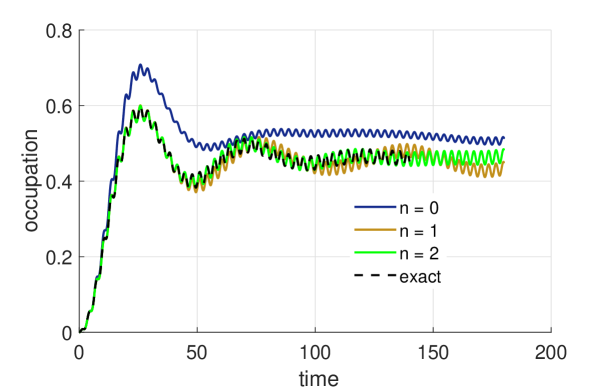
Figure 1: The spin energy level is at the center of bath’s energy band. The average occupation of the qubit is computed by exact diagonalization (in the truncated full Fock space), which required us to take into account 8 bath excitations to achieve the convergence up to the time $t=180$ (dahsed line). At the same time, the results for the dressed quantum trajectory method at $n=0$ (blue), $n=1$ (brown), and $n=2$ (green), show that we reach convergence up to the stationary regime with only 2 virtual excitations.

IV THE PROBLEM OF MEMORY TAILS

Let us simulate the system described in a previous section for a longer period of time. In Fig. 2 we present the results for zero $\left(n=0\right)$ and one $\left(n=1\right)$ virtual quantum.

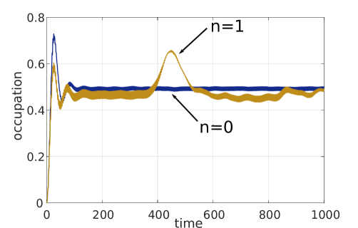
Figure 2: The same system as in previous figure, but simulated on much longer times. The cases of zero virtual quanta ($n=0$) and one virtual quantum ($n=1$) are presented. It is seen that for one virtual quantum, when a trunacted representation of the bath wavefunction appears, a revival is observed at $t\approx 400$. This is the manifestation of the generic problem of long-range memory tails.

We see that for zero virtual photons the simulation is stable and reaches the stationary non-equilibrium state. At the same time, for one virtual quantum we observe the spurious revival around $t=400$. Its emergence is not related to the truncation in the number of virtual quanta $n$. Instead, for any number of virtual quanta, due to the discretization of the bath spectrum on a finite frequency range, the tails of the memory function $M\left(\tau\right)$ get corrupted. The finer is the discretization, the more retarded part of the tail is corrupted, hence the revival is more delayed. This is a general problem of all the simulation methods. The conventional ED simulations truncate the number of the bath modes which leads to the occurence of the spurious reflected signal from the boundary. Other methods, which directly deal with the memory functions, such as path integral-based methods (QUAPI and beyond) and HOPS, directly truncate the memory tails, which also leads to corruption of calculated observables after a certain simulation time.

Next paper in this series (Polyakov and Rubtsov, 2018a) is devoted to the problem of memory tails. We show there that it is possible to devise a special soft coarsegraining of the virtual quanta wavefunction, such that revivals disappear.

V CONCULSION

In this work we propose a novel formulation for the dynamics of open quantum systems in a non-Markovian environment. In conventional approaches, the quantum field of the bath can develop large occupations of quanta, with correlations of high dimensions. This presents a formiddable obstacle both to the description of non-Markovian physics and to the development of long-time simulation methods. Here we demonstrate that the full quantum field can be divided into the two components, of different physical nature, and each with its own favourable properties. The virtual component is an intrinsically quantum object, but tends to be asymptotically bounded at large times, so that it can be efficiently simulated within a truncated basis. The second component of the quantum field, the observable part, can grow without bounds with time, but the hierarchy of its correlations have classical stochastic structure, so that its dynamics can be efficiently simulated by Monte Carlo methods.

We believe that the proposed formulation provides us with a natural solution to the problem of decomposition of the bath $B$ into the entangled memory part $M$ (the virtual quanta) and the detector part $B$ (the observable quanta). This may be useful for the analysis of various non-Markovian phenomena such as the information and energy backflow; for the discussion of various information and entanglement measures in the presence non-Markovianity.

Finally, this approach sheds light on the physical foundation of such methods as the NMQSD and HOPS, “explaining” their relative success. This may pave the way for novel, more advances, simulation techniques. In this respect one of the favourable features of the presented formulation is that its main concepts- the dressed state and its vacuum projection - are simple and well-defined quantum-mechanical objects, amenable to analysiz, combination, or approximation by any of the numerous conventional quantum-mechanical methods.

VI DERIVATION OF THE HUSIMI MASTER EQUATION

In the time derivative (27) the following terms will be zero:

$$\ldots\times\left\langle 0\right|_{\textrm{b}}\widehat{b}^{\dagger}\left|\Psi_{\textrm{dress}}\left(z,t\right)\right\rangle=0$$ (57)

and

$$\left\langle\Psi_{\textrm{dress}}\left(z,t\right)\right|\widehat{b}\left|0\right\rangle_{\textrm{b}}\times\ldots=0.$$ (58)

There will be also terms of the form

$$\ldots\times\left\langle 0\right|_{\textrm{b}}\widehat{b}\left|\Psi_{\textrm{dress}}\left(z,t\right)\right\rangle\,\,\,\textrm{and}\,\,\,\left\langle\Psi_{\textrm{dress}}\left(z,t\right)\right|\widehat{b}^{\dagger}\left|0\right\rangle_{\textrm{b}}\times\ldots,$$ (59)

which are non-zero, and we calculate them using the property (29). Another property we will use is that the quantum trajectory is analytic function of the noise:

$$\frac{\delta}{\delta z^{*}\left(\omega\right)}\left|\Psi_{\textrm{dress}}\left(z,t\right)\right\rangle=0\,\,\,\textrm{and}\,\,\,\frac{\delta}{\delta z\left(\omega\right)}\left\langle\Psi_{\textrm{dress}}\left(z,t\right)\right|=0.$$ (60)

Taking into account all these facts, we obtain for the time derivative of $Q\left(z;t\right)$:

$$\partial_{t}Q\left(z,t\right)=\exp\left(-\int d\omega\left|z\left(\omega\right)\right|^{2}\right)\left\{-iz\overline{s}_{\textrm{u}}+i\partial_{z^{*}\left(t\right)}\overline{s}_{\textrm{u}}+iz^{*}\overline{s}_{\textrm{u}}^{*}-i\partial_{z\left(t\right)}\overline{s}_{\textrm{u}}^{*}\right\},$$ (61)

where the unnormalized average of $\widehat{s}$ was introduced

$$\overline{s}_{\textrm{u}}=\left\langle\Psi_{\textrm{dress}}\left(z,t\right)\right|\left|0\right\rangle_{\textrm{b}}\widehat{s}\left\langle 0\right|_{\textrm{b}}\left|\Psi_{\textrm{dress}}\left(z,t\right)\right\rangle,$$ (62)

and the formal time derivative with respect to “instantaneous” noise value was defined (just for the brevity of notation)

$$\partial_{z\left(t\right)}\eqqcolon\intop_{-\infty}^{+\infty}d\omega c\left(\omega\right)\exp\left(-i\omega t\right)\frac{\delta}{\delta z\left(\omega\right)}.$$ (63)

To proceed further from Eq. (61), we employ the properties

$$\partial_{z\left(t\right)}\int d\omega\left|z\left(\omega\right)\right|^{2}=z^{*}\left(t\right)$$ (64)

and

$$\partial_{z\left(t\right)}\exp\left(-\int d\omega\left|z\left(\omega\right)\right|^{2}\right)=\exp\left(-\int d\omega\left|z\left(\omega\right)\right|^{2}\right)\left\{-z^{*}\left(t\right)+\partial_{z\left(t\right)}\right\}.$$ (65)

Finally, we arrive at the master equation (30).

References

- Zurek (2003) W. H. Zurek, Rev. Mod. Phys. 75, 715 (2003).
- Schlosshauer (2004) M. Schlosshauer, Rev. Mod. Phys. 76, 1267 (2004).
- Blume-Kohout and Zurek (2008) R. Blume-Kohout and W. H. Zurek, Phys. Rev. Lett. 101, 240405 (2008).
- Riedel and Zurek (2011) C. J. Riedel and W. H. Zurek, New J. Phys. 13, 073038 (2011).
- Korbicz et al. (2017) J. K. Korbicz, E. A. Aguilar, P. Cwiklinski, and P. Horodecki, Phys. Rev. A 96, 032124 (2017).
- Mironowicz et al. (2017) P. Mironowicz, J. K. Korbicz, and P. Horodecki, Phys. Rev. Lett. 118, 150501 (2017).
- Knott et al. (2018) P. A. Knott, T. Tufarelli, M. Piano, and G. Adesso, Phys. Rev. Lett. 121, 160401 (2018).
- Brandes (2010) T. Brandes, Phys. Rev. Lett. 105, 060602 (2010).
- Kiesslich et al. (2012) G. Kiesslich, C. Emary, G. Schaller, and T. Brandes, New J. Phys. 14, 123036 (2012).
- Gough (2014) J. Gough, Phys. Rev. E 90, 062109 (2014).
- Brandes and Emary (2016) T. Brandes and C. Emary, Phys. Rev. E 93, 042103 (2016).
- Luo et al. (2016) J. Y. Luo, J. Jin, S.-K. Wang, J. Hu, Y. Huang, and X.-L. He, Phys. Rev. B 93, 125122 (2016).
- Wagner et al. (2017) T. Wagner, P. Strasberg, J. C. Bayer, E. P. Rugeramigabo, T. Brandes, and R. J. Haug, Nat. Nanotechnol. 12, 218 (2017).
- Beige et al. (2000) A. Beige, D. Braun, B. Tregenna, and P. L. Knight, Phys. Rev. Lett. 85, 1762 (2000).
- Verstraete et al. (2009) F. Verstraete, M. M. Wolf, and J. I. Cirac, Nat. Phys 5, 633 (2009).
- Zanardi et al. (2016) P. Zanardi, J. Marshall, and L. C. Venuti, Phys. Rev. A 93, 022312 (2016).
- Kapit (2018) E. Kapit, Phys. Rev. Lett. 120, 050503 (2018).
- de Vega and Alonso (2017) I. de Vega and D. Alonso, Rev. Mod. Phys. 89, 015001 (2017).
- Pruschke et al. (1995) T. Pruschke, M. Jarrell, and J. Freericks, Advances in Physics 44, 187 (1995), https://doi.org/10.1080/00018739500101526 .
- Georges et al. (1996) A. Georges, G. Kotliar, W. Krauth, and M. J. Rozenberg, Rev. Mod. Phys. 68, 13 (1996).
- Freericks et al. (2006) J. K. Freericks, V. M. Turkowski, and V. Zlatic, Phys. Rev. Lett. 97, 266408 (2006).
- Aoki et al. (2014) H. Aoki, N. Tsuji, M. Eckstein, M. Kollar, T. Oka, and P. Werner, Rev. Mod. Phys. 86, 779 (2014).
- Breuer et al. (2016) H.-P. Breuer, E.-M. Laine, J. Piilo, and B. Vacchini, Rev. Mod. Phys. 88, 021002 (2016).
- Wiseman and Milburn (1993) H. M. Wiseman and G. J. Milburn, Phys. Rev. A 47, 642 (1993).
- Wiseman (1996) H. M. Wiseman, Quantum Semiclass. Opt. 8, 205 (1996).
- Percival (1999) I. Percival, Quantum State Diffusion (Cambridge University Press, Cambridge, 1999).
- Warszawski and Wiseman (2003a) P. Warszawski and H. M. Wiseman, J. Opt. B: Quantum Semiclass. Opt. 5, 1 (2003a).
- Warszawski and Wiseman (2003b) P. Warszawski and H. M. Wiseman, J. Opt. B: Quantum Semiclass. Opt. 5, 15 (2003b).
- Oxtoby et al. (2005) N. P. Oxtoby, P. Warszawski, H. M. Wiseman, H.-B. Sun, and R. E. S. Polkinghorne, Phys. Rev. B 71, 165317 (2005).
- Tilloy et al. (2015) A. Tilloy, M. Bauer, and D. Bernard, Phys. Rev. A 92, 052111 (2015).
- Bauer et al. (2015) M. Bauer, D. Bernard, and A. Tilloy, J. Phys. A: Math. Theor. 48, 25FT02 (2015).
- Daley (2014) A. J. Daley, Adv. in Phys. 63, 77 (2014).
- Zhang et al. (2017) J. Zhang, Y.-x. Liu, R.-B. Wu, K. Jacobs, and F. Nori, Physics Reports 679, 1 (2017).
- Gardiner and Collett (1985) C. W. Gardiner and M. J. Collett, Phys. Rev. A 31, 3761 (1985).
- Gardiner and Parkins (1987) C. W. Gardiner and A. S. Parkins, J. Opt. Soc. Am. B 4, 1683 (1987).
- Gardiner (2004) C. W. Gardiner, Opt. Commun 243, 57 (2004).
- Li et al. (2018) L. Li, J. W. H. Michael, and H. M. Wiseman, Phys. Rep. 759, 1 (2018).
- Jack et al. (1999) M. W. Jack, M. J. Collett, and D. F. Walls, J. Opt. B: Quantum Semiclass. Opt. 1, 452 (1999).
- Xu and Li (2018) L. Xu and X.-Q. Li, Sci. Rep. 8, 452 (2018).
- Breuer and Petruccione (2007) H.-P. Breuer and F. Petruccione, The Theory of Open Quantum Systems (Oxford University Press, Oxford, 2007).
- Diosi (2012) L. Diosi, Phys. Rev. A 85, 034101 (2012).
- Garraway (1997) B. M. Garraway, Phys. Rev. A 55, 2290 (1997).
- Mazzola et al. (2009) L. Mazzola, S. Maniscalco, J. Piilo, K.-A. Suominen, and B. M. Garraway, Phys. Rev. A 80, 012104 (2009).
- Arrigoni et al. (2013) E. Arrigoni, M. Knap, and W. v. d. Linden, Phys. Rev. Lett. 110, 086403 (2013).
- Budini (2013) A. A. Budini, Phys. Rev. A 88, 012124 (2013).
- Dorda et al. (2014) M. Dorda, Antonius amd Nuss, W. v. d. Linden, and E. Arrigoni, Phys. Rev. B 89, 165105 (2014).
- Strathearn et al. (2018) A. Strathearn, P. Kirton, D. Kilda, J. Keeling, and B. W. Lovett, Nat. Commun. 9, 3322 (2018).
- Makarov and Makri (1994) D. E. Makarov and N. Makri, Chemical Physics Letters 221, 482 (1994).
- Makri (1995) N. Makri, Journal of Mathematical Physics 36, 2430 (1995), https://doi.org/10.1063/1.531046 .
- Makri and Makarov (1995) N. Makri and D. E. Makarov, The Journal of Chemical Physics 102, 4600 (1995), https://doi.org/10.1063/1.469508 .
- Makri et al. (1996) N. Makri, E. Sim, D. E. Makarov, and M. Topaler, Proceedings of the National Academy of Sciences 93, 3926 (1996), http://www.pnas.org/content/93/9/3926.full.pdf .
- Diosi et al. (1998) L. Diosi, N. Gisin, and W. T. Strunz, Phys.l Rev. A 58, 1699 (1998).
- Suess et al. (2014) D. Suess, A. Eisfeld, and W. T. Strunz, Phys. Rev. Lett. 113, 150403 (2014).
- Hartmann and Strunz (2017) R. Hartmann and W. T. Strunz, J. Chem. Theor. Comput. 13, 5834 (2017).
- Shao (2004) J. Shao, J. Chem. Phys. 120, 5053 (2004).
- Yan et al. (2004) Y.-a. Yan, F. Yang, Y. Liu, and J. Shao, Chem. Phys. Lett. 395, 216 (2004).
- Zhou and Shao (2008) Y. Zhou and J. Shao, J. Chem. Phys. 128, 034106 (2008).
- Yan and Shao (2016) Y.-A. Yan and J. Shao, Front. Phys. 11, 110309 (2016).
- Polyakov and Rubtsov (2018a) E. A. Polyakov and A. N. Rubtsov, “Information loss pathways in a nuremically exact simulation of a non-markovian open quantum system,” (2018a), to be published.
- (60) E. A. Polyakov and A. N. Rubtsov, “Stochastic dressed wavefunction: a numerically exact solver for bosonic impurity model dynamics within wide time interval,” arXiv:1712.04279 [cond-mat] .
- Polyakov and Rubtsov (2018b) E. A. Polyakov and A. N. Rubtsov, AIP Conf. Proc. 1936, 020028 (2018b).
- Tanimura (1990) Y. Tanimura, Phys. Rev. A 41, 6676 (1990).
- Breuer (2007) H.-P. Breuer, Phys. Rev. A 75, 022103 (2007).
- Note (1) Here is understood as the limit for a discretization of the frequency axis , and are understood as real and imaginary parts correspondingly of the complex number .
- Milonni (1993) P. W. Milonni, The quantum vacuum: an introduction to quantum electrodynamics (Academic Press, London, 1993).
- Holstein (1959) T. Holstein, Ann. Phys. (NY) 8, 325 (1959).