Abstract

We revisit the basic properties of Fano-Feshbach resonances in two-body systems with van der Waals tail interactions, such as ultracold neutral atoms. Using a two-channel model and two different methods, we investigate the relationship between the width and shift of the resonances and their dependence on the low-energy parameters of the system. Unlike what was previously believed [Rev. Mod. Phys. 82, 1225 (2010)] for magnetic resonances, we find that the ratio between the width and the shift of a resonance does not depend only on the background scattering length, but also on a closed-channel scattering length. We obtain different limits corresponding to different cases of optical and magnetic resonances. Although the generalisation of the theory to the multi-channel case remains to be done, we found that our two-channel predictions are verified for a specific resonance of lithium-6.

1 Introduction

A Fano-Feshbach resonance [1, 2] is the strong modification of the scattering properties of two particles due to their coupling with a bound state in a different internal state. At low energy where the s-wave scattering is dominant, these resonances cause the scattering length of the two particles to diverge. While such resonances may accidentally occur in nature [3], it was realised that they could be induced in ultracold alkali atoms by applying a magnetic field to these systems [4]. Because of different Zeeman shifts experienced by different hyperfine states of atoms, it is possible to tune the intensity of the magnetic field such that a bound state in a certain hyperfine state approaches the scattering energy of the two atoms, resulting in a Fano-Feshbach resonance. This led to one of the major achievements in the field of ultracold atoms, the possibility to control their interactions, enabling the experimental study of a wealth of fundamental quantum phenomena for over nearly two decades [5, 6, 7, 8, 9, 10, 11, 12, 13].

The general formalism of Fano-Feshbach resonances has already been studied in detail [1, 2, 14, 15]. This work focuses on the general relationship between the width and shift characterising Fano-Feshbach resonances. In section 2 of this article, we introduce the two-channel model which is used afterwards to derive analytic relations. In section 3 we recall how the shift and width of the resonance can be deduced in the isolated resonance approximation. In section 4 and 5, we establish the relationship between the shift $\Delta$ and the width $\Gamma$, in particular for systems characterised at large interparticle distance by a van der Waals interaction.

Our main result shows the dependence of these quantities upon the open-channel (background) scattering length $a_{{\rm bg}}$ and a closed-channel scattering length $a_{{\rm c}}$:

$$\Delta \propto\left(a_{{\rm bg}}-a_{{\rm c}}\right),\qquad\Gamma\propto\left(a_{{\rm bg}}-a_{{\rm c}}\right)^{2}.$$ (1)

This result is inconsistent with the formula given by Eq. (37) of Ref. [15] obtained from multi-channel quantum defect theory (MQDT). To clarify this discrepancy, in section 6 we use the MQDT approach to rederive the width and shift. This derivation turns out to confirm our results obtained with the isolated resonance approximation. Moreover, we show that the formula of Ref. [15] relies on a simplifying assumption that appears to be invalid in general. Finally, in section 8, we illustrate our results with the broad magnetic resonance of lithium-6 atoms.

2 The two-channel model

The simplest description of Fano-Feshbach resonances requires two channels, corresponding to two different internal states of a pair of atoms. Each channel is associated with a different interaction potential between the two atoms. At large distances, these two potentials tend to different energies, or thresholds, which are equal to the energies of two separated atoms in the internal states of the corresponding channel. For a resonance to occur, the initially separated atoms must scatter with a relative kinetic energy that is above the threshold of one channel, called the open channel, but below the threshold of the other channel, called the closed channel. In addition, the relative motion of the atoms in one channel must be coupled to that of the other channel. The wave function for the relative vector ${\bm{R}}$ between the two atoms with relative kinetic energy $E$ is therefore described by two components ${\Psi_{{\rm o}}(\bm{R})}$ and ${\Psi_{{\rm c}}(\bm{R})}$, respectively for the open and the closed channel, satisfying the coupled Schrödinger equations (in ket notation):

$$\left(T+V_{{\rm oo}}-E\right)|\Psi_{{\rm o}}\rangle+V_{{\rm oc}}|\Psi_{{\rm c}}\rangle=0$$ (2)

$$\left(T+V_{{\rm cc}}-E\right)|\Psi_{{\rm c}}\rangle+V_{{\rm co}}|\Psi_{{\rm o}}\rangle=0,$$ (3)

where ${V_{{\rm oo}}}$ and ${V_{{\rm cc}}}$ are the open- and closed-channel potentials with ${V_{{\rm cc}}(\infty)>E>V_{{\rm oo}}(\infty)}$, and ${V_{{\rm oc}}=V_{{\rm co}}^{*}}$ are the coupling potentials. In Eqs. (2,3) $T$ is the relative kinetic energy operator,

$$T=-\frac{\hbar^{2}}{2\mu}\nabla_{\bm{R}}^{2},$$ (4)

where $\mu$ is the reduced mass of the atoms. For convenience, we choose ${V_{{\rm oo}}(\infty)=0}$. Equations (2) and (3) can be integrated as follows:

$$|\Psi_{{\rm o}}\rangle =|\bar{\Psi}_{{\rm o}}^{E}\rangle+G_{{\rm o}}^{+}V_{{\rm oc}}|\Psi_{{\rm c}}\rangle$$ (5)

$$|\Psi_{{\rm c}}\rangle =0+G_{{\rm c}}V_{{\rm co}}|\Psi_{{\rm o}}\rangle,$$ (6)

where ${G_{{\rm o}}^{+}=\left(E+i0^{+}-T-V_{{\rm oo}}\right)^{-1}}$ and ${G_{{\rm c}}=\left(E-T-V_{{\rm cc}}\right)^{-1}}$ are the resolvents of the open and closed channels, and ${|\bar{\Psi}_{{\rm o}}^{E}\rangle}$ is the scattering eigenstate of the open-channel Hamiltonian ${T+V_{{\rm oo}}}$ at energy $E$. It is energy-normalised, i.e., ${\langle\bar{\Psi}_{{\rm o}}^{E}|\bar{\Psi}_{{\rm o}}^{E^{\prime}}\rangle=\delta(E-E^{\prime})}$.

3 Shift and width of an isolated resonance

The description of a Fano-Feshbach resonance is usually done in the isolated resonance approximation [14, 16, 17]. In that approximation, only a single bound state ${|\Psi_{m}\rangle}$ (here assumed with s-wave symmetry) of the closed channel gives a significant contribution to the resonance. The closed-channel resolvent may therefore be decomposed into a resonant and a non-resonant part:

$$G_{{\rm c}}=\frac{|\Psi_{m}\rangle\langle\Psi_{m}|}{E-E_{m}}+\underbrace{\sum_{n\neq m}\frac{|\Psi_{n}\rangle\langle\Psi_{n}|}{E-E_{n}}}_{G_{{\rm c}}^{\text{nr}}},$$ (7)

where ${|\Psi_{n}\rangle}$ and ${E_{n}}$ denote all the eigenstates and energies of the closed-channel Hamiltonian ${T+V_{{\rm cc}}}$, normalised as ${\langle\Psi_{n}|\Psi_{n^{\prime}}\rangle=\delta_{n,n^{\prime}}}$. One finds

$$|\Psi_{{\rm o}}\rangle=|\Psi_{\text{{\rm bg}}}\rangle+G_{{\rm o}}^{+}T_{{\rm res}}|\Psi_{{\rm bg}}\rangle$$ (8)

$$|\Psi_{{\rm c}}\rangle=|\Psi_{m}\rangle\frac{\langle\Psi_{m}|V_{{\rm co}}|\Psi_{{\rm o}}\rangle}{E-E_{m}}+G_{{\rm c}}^{{\rm nr}}V_{{\rm co}}|\Psi_{{\rm o}}\rangle,$$ (9)

where we have introduced the background scattering state ${|\Psi_{{\rm bg}}\rangle}$ and the operator ${T_{{\rm res}}}$ given by

$$|\Psi_{{\rm bg}}\rangle =|\bar{\Psi}_{{\rm o}}^{E}\rangle+G_{{\rm o}}^{+}V_{{\rm oc}}G_{{\rm c}}^{\text{nr}}V_{{\rm co}}|\Psi_{{\rm o}}\rangle$$ (10)

$$T_{{\rm res}} =\frac{V_{{\rm oc}}|\Psi_{m}\rangle\langle\Psi_{m}|V_{{\rm co}}}{E-E_{m}-\langle\Psi_{m}|V_{{\rm co}}G_{{\rm o}}^{+}V_{{\rm oc}}|\Psi_{m}\rangle}.$$ (11)

Equation (8) shows that ${|\Psi_{{\rm o}}\rangle}$ is analogous to a scattering state in a single-channel problem, where ${|\Psi_{{\rm bg}}\rangle}$ plays the role of the incident state, and ${T_{\text{res}}}$ is the transition operator. In this single-channel picture, the scattering amplitude is thus proportional to the matrix element ${\langle\Psi_{{\rm bg}}|T_{{\rm res}}|\Psi_{{\rm bg}}\rangle}$ of this transition operator for the incident state. From Eqs. (8-11) we have

$$\langle\Psi_{{\rm bg}}|T_{{\rm res}}|\Psi_{{\rm bg}}\rangle=\frac{\Gamma}{2\pi}\frac{1}{E-E_{m}-\Delta+i\Gamma^{\prime}/2},$$ (12)

where $\Delta$ and $\Gamma$ are given by

$$\Delta=\langle\Psi_{m}|V_{{\rm co}}{\rm Re}{(G_{{\rm o}}^{+})}V_{{\rm oc}}|\Psi_{m}\rangle$$ (13)

$$\Gamma=2\pi|\langle\Psi_{m}|V_{{\rm co}}|\Psi_{{\rm bg}}\rangle|^{2},$$ (14)

and ${\Gamma^{\prime}=2\pi|\langle\Psi_{m}|V_{{\rm co}}|\bar{\Psi}_{{\rm o}}^{E}\rangle|^{2}}$. In the isolated resonance approximation, whenever the scattering energy $E$ is close to the molecular energy, the molecular states ${n\neq m}$ only bring a small correction to the closed-channel state in Eq. (9) and to the background scattering state in Eq. (10). One can thus make the approximation ${|\Psi_{{\rm c}}\rangle\propto|\Psi_{m}\rangle}$ and ${|\Psi_{{\rm bg}}\rangle\approx|\bar{\Psi}_{{\rm o}}^{E}\rangle}$ yielding ${\Gamma^{\prime}\approx\Gamma}$. We can then identify a Breit-Wigner law in Eq. (12) with the width ${\Gamma}$ and shift ${\Delta}$. From Eq. (8), one finds the s-wave scattering phase shift,

$$\eta=\eta_{{\rm bg}}+\eta_{\text{res}}$$ (15)

where ${\eta_{{\rm bg}}}$ is the background scattering phase shift contained in ${|\psi_{{\rm bg}}\rangle}$ and ${\eta_{\text{res}}}$ is the resonant scattering phase shift given by the resonant K-matrix ${K_{\text{res}}=\tan\eta_{\text{res}}}$ of the Breit-Wigner form,

$$K_{\text{res}}=-\frac{\Gamma/2}{E-E_{m}-\Delta}.$$ (16)

In the limit of low energy ${E=\frac{\hbar^{2}k^{2}}{2\mu}}$, the scattering length ${a=-\lim_{k\to 0}\tan\eta/k}$ is therefore

$$a=a_{{\rm bg}}-\frac{\lim_{k\to 0}\Gamma/2k}{E_{m}+\Delta}.$$ (17)

The scattering length ${a_{{\rm bg}}}$, the width $\Gamma$, and shift $\Delta$ are thus the parameters that characterise the Fano-Feshbach resonance at low energy. In the rest of this paper, we consider $\Gamma$ and $\Delta$ in the limit of low scattering energy.

The isolated resonance approximation is valid in the limit of small coupling ${V_{{\rm co}}}$ with respect to level spacings in the closed channel, so that effectively the resonant molecular level is well isolated from the other levels. Indeed, the condition ${|\langle\Psi_{m}|\Psi_{{\rm c}}\rangle|\gg|\langle\Psi_{n}|\Psi_{{\rm c}}\rangle|}$ needed to ensure that ${|\Psi_{{\rm c}}\rangle}$ is approximately proportional to ${|\Psi_{m}\rangle}$ gives the requirement

$$|\tilde{E}_{m}-\tilde{E}_{n}|\gg\pi|\langle\Psi_{n}|V_{{\rm co}}|\Psi_{{\rm bg}}\rangle\langle\Psi_{m}|V_{{\rm co}}|\Psi_{{\rm bg}}\rangle|,$$ (18)

where ${\tilde{E}_{m}=E_{m}+\langle\Psi_{m}|V_{{\rm co}}G_{0}^{+}V_{{\rm oc}}|\Psi_{m}\rangle}$ and ${\tilde{E}_{n}=E_{n}+\langle\Psi_{n}|V_{{\rm co}}G_{0}^{+}V_{{\rm oc}}|\Psi_{m}\rangle}$ are the dressed energies of the closed-channel molecular levels. We call the regime where the inequality in Eq. (18) is satisfied the diabatic limit.

Even for large couplings $V_{co}$, it may be possible to apply the isolated resonance in another basis for which the new coupling becomes small. One such basis is the adiabatic basis that diagonalises at each separation ${R}$ the potential matrix ${V_{ij}}$. The resulting equations are formally similar to the original equations, where the potentials ${V_{{\rm oo}}}$ and ${V_{{\rm cc}}}$ are replaced by the adiabatic potentials ${V_{{\rm oo}}^{\prime}}$ and ${V_{{\rm cc}}^{\prime}}$, and the couplings ${V_{{\rm oc}}}$ and ${V_{{\rm co}}}$ are replaced by radial couplings ${V_{{\rm oc}}^{\prime}=-V_{{\rm co}}^{\prime}}$ of the form (see Appendix 1)

$$V_{{\rm oc}}^{\prime}(R)=-\frac{\hbar^{2}}{2\mu}\left[2\frac{Q(R)}{R}\frac{d}{dR}(R\cdot)+\frac{dQ(R)}{dR}\right],$$ (19)

where the function ${Q(R)}$ in Eq. (19) is given by

$$Q(R)=-\frac{1}{2}\frac{d}{dR}\left[\arctan\left(\frac{2V_{{\rm oc}}(R)}{V_{{\rm oo}}(R)-V_{{\rm cc}}(R)}\right)\right].$$ (20)

If the coupling $V_{{\rm oc}}^{\prime}$ happens to be small enough, the condition (18) written in the new basis may be satisfied and the isolated resonance approximation may be applied again with a bound state ${|\Psi_{m}^{\prime}\rangle}$ among the family of bound states ${|\Psi_{n}^{\prime}\rangle}$ in the new closed channel. We call this regime of weak adiabatic coupling the adiabatic limit.

4 General dependence on ${a_{{\rm bg}}}$

We first consider the dependence of the width upon the background scattering length for a vanishing colliding energy. Due to the isotropic character of the inter-channel coupling, only the s-wave component of the background scattering state contributes in Eq. (14). At zero scattering energy, the s-wave component ${[\Psi_{{\rm bg}}(R)]_{s}}$ of the background state ${|\Psi_{{\rm bg}}\rangle}$ can be written in terms of radial functions as

$$\left[\Psi_{{\rm bg}}(\bm{R})\right]_{{\rm s}}\equiv\int\frac{d\Omega_{\bm{R}}}{4\pi}\langle\bm{R}|\Psi_{{\rm bg}}\rangle\propto\frac{u_{0}(R)-a_{{\rm bg}}u_{\infty}(R)}{R},$$ (21)

where the integration over the solid angle ${\Omega_{\bm{R}}}$ selects the s-wave component, and the radial functions ${u_{0}}$ and ${u_{\infty}}$ are two independent solutions of the open-channel radial equation,

$$\left(-\frac{\hbar^{2}}{2\mu}\frac{d^{2}}{dR^{2}}+V_{{\rm oo}}(R)\right)u(R)=0$$ (22)

with the asymptotic boundary conditions ${u_{0}(R)\xrightarrow[R\to\infty]{}R}$ and ${u_{\infty}(R)\xrightarrow[R\to\infty]{}1}$. The linear combination of these two functions in Eq. (21) corresponds precisely to the physical solution of (22) that is regular at the origin. It is then clear from Eq. (14) and (21) that the width ${\Gamma}$ is the square of a quantity varying linearly with ${a_{{\rm bg}}}$. In particular, for some value of ${a_{{\rm bg}}}$, the width ${\Gamma}$ vanishes.

Second, we examine the dependence of the shift of the resonance as a function of the background scattering length. For this purpose, we use the Green’s function of the s-wave radial Schrödinger equation for the open channel,

$$\left(-\frac{\hbar^{2}}{2\mu}\frac{d^{2}}{dR^{2}}+V_{{\rm oo}}(R)-E\right){\mathcal{G}}_{{\rm o}}^{E}(R,R^{\prime})=-\delta(R-R^{\prime}).$$ (23)

It is related to the resolvent by

$${\mathcal{G}}_{{\rm o}}^{E}(R,R^{\prime})=4\pi RR^{\prime}\left[G_{{\rm o}}(\bm{R},\bm{R}^{\prime})\right]_{s}\equiv RR^{\prime}\int d\Omega_{\bm{R}}\langle\bm{R}|G_{{\rm o}}^{+}|\bm{R}^{\prime}\rangle.$$ (24)

In the following, we will focus on the low-energy regime. In this regime, the Green’s function ${\mathcal{G}_{{\rm o}}^{E}(R,R^{\prime})}$ is well approximated at short distances ${R,R^{\prime}\ll k^{-1}}$ by its zero-energy limit,

$${\mathcal{G}}_{{\rm o}}^{0}(R,R^{\prime})=\\ -\frac{2\mu}{\hbar^{2}}\begin{cases}\left(u_{0}(R)-a_{{\rm bg}}u_{\infty}(R)\right)u_{\infty}(R^{\prime})&\ \text{for }R<R^{\prime}\\ \left(u_{0}(R^{\prime})-a_{{\rm bg}}u_{\infty}(R^{\prime})\right)u_{\infty}(R)&\ \text{for }R>R^{\prime}\end{cases}.$$ (25)

Using this last expression, it follows from Eq. (13) that the shift $\Delta$ varies linearly with ${a_{{\rm bg}}}$.

5 Case of van der Waals interactions

Neutral atoms in their ground state interact via interactions that decay as ${-C_{6}/R^{6}}$ (van der Waals potential) beyond a certain radius $R_{0}$. In this case, one can give the explicit dependence of the width and shift on ${a_{{\rm bg}}}$. The van der Waals tail introduces a natural length scale ${R_{{\rm vdW}}}$ (or energy ${E_{{\rm vdW}}}$) denoted as the van der Waals length (or energy):

$$R_{{\rm vdW}}=\frac{1}{2}\left(\frac{2\mu C_{6}}{\hbar^{2}}\right)^{1/4}\ ;\ E_{{\rm vdW}}=\frac{\hbar^{2}}{2\mu R_{{\rm vdW}}^{2}}.$$ (26)

In what follows, we will also use the Gribakin-Flambaum mean scattering length ${\bar{a}=4\pi/\Gamma(1/4)^{2}R_{{\rm vdW}}}$ where ${\Gamma(\cdot)}$ denotes the Gamma function, giving ${\bar{a}\approx 0.955978...R_{{\rm vdW}}}$ [18]. The radial functions ${u_{0}(R)}$ and ${u_{\infty}(R)}$ are known analytically in the region ${R>R_{0}}$ of the van der Waals tail:

$$u_{0}(R)/R_{{\rm vdW}} =\sqrt{x}\Gamma(3/4)J_{-1/4}(2x^{-2})$$ (27)

$$u_{\infty}(R) =\sqrt{x}\Gamma(5/4)J_{1/4}(2x^{-2}),$$ (28)

where ${x=R/R_{{\rm vdW}}}$ and $J$ denotes the Bessel function. In practice, ${R_{0}<R_{{\rm vdW}}}$ and in the short-range region ${R_{0}<R\lesssim R_{{\rm vdW}}}$, the functions exhibit rapid oscillations that are well approximated by the semi-classical formulas,

$$u_{0}(R)/R_{{\rm vdW}} \approx\Gamma(3/4)\frac{x^{3/2}}{\sqrt{\pi}}\cos(2x^{-2}-\pi/8)$$ (29)

$$u_{\infty}(R) \approx\Gamma(5/4)\frac{x^{3/2}}{\sqrt{\pi}}\cos(2x^{-2}-3\pi/8).$$ (30)

One deduces from Eq. (14) and the normalization factor of the scattering state ${\bar{\Psi}_{{\rm o}}^{E}}$, that the resonance width vanishes at zero energy with a linear law in the colliding momentum ${k=\sqrt{2\mu E}/\hbar}$. Thus, in the limit of small ${k}$, one finds the explicit dependence of $\Gamma$ and $\Delta$ upon ${a_{{\rm bg}}}$:

$$\frac{\Gamma}{2k\bar{a}} =\pi E_{{\rm vdW}}\times\left|\sqrt{2}A-r_{{\rm bg}}B\right|^{2}$$ (31)

$$\Delta =-\pi E_{{\rm vdW}}\times\Bigg{[}\sqrt{2}C-r_{{\rm bg}}B^{2}\Bigg{]},$$ (32)

where we introduced the reduced background scattering length ${r_{{\rm bg}}=a_{{\rm bg}}/\bar{a}}$, and the coefficients

$$A =\int_{0}^{\infty}dxw(x)x^{3/2}\cos(2x^{-2}-\pi/8)$$ (33)

$$B =\int_{0}^{\infty}dxw(x)x^{3/2}\cos(2x^{-2}-3\pi/8)$$

$$C =\int_{0}^{\infty}dxw(x)x^{3/2}\cos(2x^{-2}-3\pi/8)$$ (34)

$$\quad\times\int_{0}^{x}dx^{\prime}\cos(2x^{\prime-2}-\pi/8)w(x^{\prime})x^{\prime 3/2}$$

$$\quad+\int_{0}^{\infty}dxw(x)x^{3/2}\cos(2x^{-2}-\pi/8)$$

$$\quad\times\int_{x}^{\infty}dx^{\prime}\cos(2x^{\prime-2}-3\pi/8)w(x^{\prime})x^{\prime 3/2}$$

with ${w(x)=\sqrt{R_{{\rm vdW}}}E_{{\rm vdW}}^{-1}R\,W(R)}$ and ${W(R)=\left[V_{{\rm oc}}\Psi_{m}(\bm{R})\right]_{s}}$.

5.1 Optical Fano-Feshbach resonance

In the case of an optical Fano-Feshbach resonance, the closed-channel potential ${V_{{\rm cc}}(R)}$ typically decays as ${V_{\text{cc}}(\infty)-C_{3}/R^{3}}$ (for pairs of alkali atoms in the ${S-P}$ electronic state). As a result, the molecular state ${\Psi_{m}}$ is usually localised near the Condon point ${R_{{\rm c}}}$ [19], so that one can make the approximation ${w(x)\approx w_{{\rm c}}\delta(x-x_{{\rm c}})}$, with the obvious notation ${x_{{\rm c}}=R_{{\rm c}}/R_{{\rm vdW}}}$. This gives:

$$A =w_{{\rm c}}x_{{\rm c}}^{3/2}\cos(2x_{{\rm c}}^{-2}-\pi/8)$$ (35)

$$B =w_{{\rm c}}x_{{\rm c}}^{3/2}\cos(2x_{{\rm c}}^{-2}-3\pi/8)$$ (36)

$$C =AB.$$ (37)

Therefore

$$\frac{\Gamma}{2k\bar{a}}=\pi E_{{\rm vdW}}\times\left|\sqrt{2}A-r_{{\rm bg}}B\right|^{2}$$ (38)

$$\Delta=-\pi E_{{\rm vdW}}\times\Bigg{[}\sqrt{2}A-r_{{\rm bg}}B\Bigg{]}B.$$ (39)

These formulae are akin to equations (3.6) and (3.7) in Ref. [19]. This gives a simple relation between $\Delta$ and ${\Gamma/2k\bar{a}}$:

$$\Delta=\frac{\Gamma}{2k\bar{a}}\times\left(r_{{\rm bg}}+\tan(2x_{{\rm c}}^{-2}-3\pi/8)-1\right)^{-1}.$$ (40)

This relation holds as long as ${R_{{\rm c}}\ll R_{{\rm vdW}}}$. For larger Condon points, one has to use the general forms (27) and (28) of ${u_{0}}$ and ${u_{\infty}}$, which gives

$$\boxed{\Delta=\frac{\Gamma}{2k\bar{a}}\times\left(r_{{\rm bg}}-\sqrt{2}\frac{J_{-1/4}(2x_{{\rm c}}^{-2})}{J_{1/4}(2x_{{\rm c}}^{-2})}\right)^{-1}}\\ \xrightarrow[r_{{\rm c}}\gg R_{{\rm vdW}}]{}\frac{\Gamma}{2k}\times(a_{{\rm bg}}-R_{{\rm c}})^{-1}.$$ (41)

5.2 Magnetic Fano-Feshbach resonance

In the case of magnetic Fano-Feshbach resonances, the closed-channel potential ${V_{{\rm cc}}(R)}$ has the same van der Waals tail as the open-channel potential, i.e. $V_{\text{cc}}(R)=V_{\text{cc}}(\infty)-C_{6}/R^{6}$ for ${R>R_{0}}$. We assume that the molecular state involved in the resonance is not too deeply bound in the closed channel, such that its probability density is significant in the van der Waals region $R>R_{0}$. This means that its binding energy $E_{b}=|E_{m}-V_{\text{cc}}(\infty)|$ is much smaller than $C_{6}/R_{0}^{6}$. In practice, $R_{0}\sim 0.4\,R_{\text{vdW}}$, which limits our consideration to $E_{b}\ll 4000\,E_{\text{vdW}}$, i.e. typically the last or next-to-last molecular level of the closed-channel potential [15]. This situation is often the case in practice. Indeed, the molecular state binding energy $E_{b}$ must be close to the energy separation $|V_{\text{oo}}(\infty)-V_{\text{cc}}(\infty)|$ between the two channel thresholds. This separation results from Zeeman and hyperfine splittings which are at most a few GHz for typical magnetic fields less than $1000$ G. Since $E_{\text{vdW}}$ typically ranges from 2 to 600 MHz for alkali atoms [15], the condition $E_{b}\lesssim 4000\,E_{\text{vdW}}$ is often satisfied.

In the interval of radii ${[R_{0},\sim\text{min}(1/\kappa,\;R_{\text{vdW}})]}$ where $\kappa=\sqrt{2\mu E_{b}/\hbar}$, the closed-channel potential is well approximated by the van der Waals tail and the shape of the molecular wave function is nearly energy-independent. In this interval, the molecular wave function ${\Psi_{m}(R)=\langle\bm{R}|\Psi_{m}\rangle}$ may be approximated by the following zero-energy formula, similar to Eq. (21),

$$\Psi_{m}(R)\propto\frac{u_{0}(R)-a_{{\rm c}}u_{\infty}(R)}{R},$$ (42)

where the radial functions $u_{0}(R)$ and $u_{\infty}(R)$ are given in this interval by the semi-classical formulas in Eqs. (29) and (30). In Eq. (42) we have introduced the length ${a_{{\rm c}}}$ that sets the phase in the semi-classical region where the wave function of the bound state oscillates. In the interval considered and in the small energy limit, all the eigenfunctions of the closed channel have the same shape and thus, in analogy with Eq. (21) for the open channel, we call ${a_{{\rm c}}}$ the closed-channel scattering length. It is, in general, different from the open-channel scattering length ${a_{{\rm bg}}}$.

In what follows, we make the additional assumption that the inter-channel coupling can be neglected beyond a certain radius ${R_{{\rm free}}}$ satisfying the condition

$$R_{0}<R_{{\rm free}}<\min(1/\kappa,\,R_{{\rm vdW}}),$$ (43)

which is usually the case for magnetic resonances. As we shall see, the crucial point is that the wave functions admit several oscillations between $R_{0}$ and ${R_{{\rm free}}}$. Let us now consider the adiabatic and diabatic limits.

5.2.1 Adiabatic limit

In the adiabatic basis, the inter-channel coupling is given by the radial coupling ${V_{{\rm co}}^{\prime}}$ of Eq. (19). Therefore we have

$$W(R) =-\frac{\hbar^{2}}{2\mu R}\left[\frac{dQ}{dR}+2Q\frac{d}{dR}\right](R\Psi_{m}(R))$$ (44)

$$\approx-\frac{\hbar^{2}}{\mu R}Q(R)\frac{d}{dR}(R\Psi_{m}(R)).$$

We assume that the function ${W(R)}$ takes negligible values for radii less than ${R_{0}}$ and that it is localised in a region where the formula Eq. (42) is often a good approximation for the molecular state ${\Psi_{m}}$ [20]. It follows that for ${{R_{0}}/{R_{{\rm vdW}}}<x<{R_{{\rm free}}}/{R_{{\rm vdW}}}}$ ,

$$w(x)=-\mathcal{W}(x)x^{-3/2}\times\\ \Big{(}\sqrt{2}\sin(2x^{-2}-\pi/8)-r_{{\rm c}}\sin(2x^{-2}-3\pi/8)\Big{)}$$ (45)

where ${\mathcal{W}(x)=\lambda_{m}R_{{\rm vdW}}Q(R)}$ and ${\lambda_{m}}$ is a dimensionless normalisation factor depending on the molecular wave function ${\Psi_{m}}$. We assume that ${\mathcal{W}(x)}$ has a support that comprises several oscillations of ${\Psi_{m}(R)}$ and is varying slowly with respect to these oscillations. Replacing the expression of Eq. (45) into Eqs. (33,34), and neglecting the terms with fast oscillations, one finds:

$$\frac{\Gamma}{2k\bar{a}} =E_{{\rm vdW}}\times\frac{\pi}{4}\overline{\mathcal{W}}^{2}\left|r_{{\rm c}}-r_{{\rm bg}}\right|^{2}$$ (46)

$$\Delta =-E_{{\rm vdW}}\times\frac{\pi}{4}\overline{\mathcal{W}}^{2}\left(r_{{\rm c}}-r_{{\rm bg}}\right),$$ (47)

where ${r_{{\rm c}}=a_{{\rm c}}/\bar{a}}$ and ${r_{{\rm bg}}=a_{{\rm bg}}/\bar{a}}$ and

$$\overline{\mathcal{W}}=\int_{R_{0}/R_{{\rm vdW}}}^{R_{{\rm free}}/R_{{\rm vdW}}}dx\,\mathcal{W}(x)=\lambda_{m}\int_{R_{0}}^{R_{{\rm free}}}dR\,Q(R).$$ (48)

These expressions are consistent with the fact that the width and shift vanish when the scattering lengths of the open and closed channels are the same. Indeed, in the coupling region, both the open- and closed-channel wave functions have the same short-range oscillations with the same phase, and since the radial coupling operator shifts the phase of one of them by ${\pi/2}$ through the derivative ${d/dR}$, the resulting overlap is zero. From Eqs. (46-47), we obtain the low-energy relation between the width and the shift:

$$\boxed{\Delta=\frac{\Gamma}{2k\bar{a}}\times(r_{{\rm bg}}-r_{{\rm c}})^{-1}}.$$ (49)

This simple relation constitutes the main result of this paper. We note in passing that it has a form similar to the relation obtained for optical resonances - see Eq. (41).

5.2.2 Diabatic limit

In the diabatic basis, the inter-channel coupling ${V_{{\rm co}}}$ is typically proportional to the exchange energy, i.e. the difference between the triplet and singlet potentials for alkali atoms, which decays exponentially with atomic separation. It is therefore localised at separations smaller than the van der Waals length, in a region that usually depends on the short-range details of the potentials. There is therefore no obvious simplification from the formulas (31) and (32) in general.

5.3 Comparison with other works

Our previous results, in particular Eq. (49), are inconsistent with formula (37) of Ref. [15], which reads as

$$\Delta=\frac{\Gamma}{2k\bar{a}}\times\frac{r_{{\rm bg}}-1}{1+(r_{{\rm bg}}-1)^{2}}.$$ (50)

Other works [21, 22] have provided expressions of $\Delta$ and $\Gamma/2k$ (see Eqs. 1.47 and 1.48 of Ref. [22]) that lead to

$$\Delta=\frac{\Gamma}{2k}\times(a_{bg}-r_{0})^{-1}$$ (51)

where $r_{0}$ is a length scale associated with the range of the open-channel interaction, i.e. typically of the order of $\bar{a}$.

Most strikingly, none of the above formulas depend on the closed channel, unlike Eq. (49) which depends on $a_{\text{c}}$. The formula of Eq. (51) was derived under the approximation that the low-energy scattering properties of the open channel are dominated by a pole (bound state) near its threshold, neglecting contributions from other poles in the Mittag-Leffler expansion of the resolvent $G_{\text{o}}$. This approximation seems to be valid only for large $a_{\text{bg}}$, and one can check that in this limit, both Eq. (51) and our result Eq. (49) indeed tend to the same limit. On the other hand, the formula of Eq. (50) is supposed to be valid for any value of $a_{\text{bg}}$ and without any particular assumption on the closed channel. It was first published in Eq. (32) of Ref. [23], and stated to be derived from the MQDT. To understand the discrepancy with our result, we now treat the two-channel resonance problem using the MQDT.

6 Multi-channel quantum defect theory

We present here a self-contained derivation of the MQDT, following the approach of Refs. [24, 25].

6.1 MQDT setup

6.1.1 Reference functions and short-range Y-matrix

The coupled radial equations for the s-wave component of Eqs. (2-3) read as follows,

$$\left(-\frac{\hbar^{2}}{2\mu}\frac{d^{2}}{dR^{2}}+V_{{\rm oo}}(R)-E\right)\psi_{{\rm o}}(R)+V_{{\rm oc}}(R)\psi_{{\rm c}}(R)=0$$ (52)

$$\left(-\frac{\hbar^{2}}{2\mu}\frac{d^{2}}{dR^{2}}+V_{{\rm cc}}(R)-E\right)\psi_{{\rm c}}(R)+V_{{\rm co}}(R)\psi_{{\rm o}}(R)=0,$$ (53)

where ${\psi_{{\rm o}}(R)=R[\Psi_{{\rm o}}(\bm{R})]_{s}}$ and ${\psi_{{\rm c}}(R)=R[\Psi_{{\rm c}}(\bm{R})]_{s}}$ are the s-wave radial wave functions. The starting point of MQDT is that the channels are uncoupled for radii ${R>R_{{\rm free}}}$. In this region, one can express the two independent solutions ${\psi^{(1)}=(\psi_{{\rm o}}^{(1)},\psi_{{\rm c}}^{(1)})}$ and ${\psi^{(2)}=(\psi_{{\rm o}}^{(2)},\psi_{{\rm c}}^{(2)})}$ of Eqs. (52),(53), as linear combinations of reference functions (${\hat{f}_{{\rm o}},\hat{g}_{{\rm o}}}$) and ${(\hat{f}_{{\rm c}},\hat{g}_{{\rm c}})}$, which are solutions of the diagonal potentials ${V_{{\rm oo}}}$ and ${V_{{\rm cc}}}$ in each channel at energy $E$:

$$\left(\begin{array}[]{cc}\psi_{{\rm o}}^{(1)}&\psi_{{\rm o}}^{(2)}\\ \psi_{{\rm c}}^{(1)}&\psi_{{\rm c}}^{(2)}\end{array}\right)=\left(\begin{array}[]{cc}\hat{f}_{{\rm o}}-\hat{g}_{{\rm o}}Y_{{\rm oo}}&\qquad-\hat{g}_{{\rm o}}Y_{{\rm oc}}\\ -\hat{g}_{{\rm c}}Y_{{\rm co}}&\qquad\hat{f}_{{\rm c}}-\hat{g}_{{\rm c}}Y_{{\rm cc}}\end{array}\right)$$ (54)

The functions ${\hat{f}_{{\rm o}}}$ and ${\hat{f}_{{\rm c}}}$ are taken to be regular at the origin, i.e. they vanish at ${R=0}$, and therefore the functions ${\hat{g}_{{\rm o}}}$ and ${\hat{g}_{{\rm c}}}$ must be irregular. They are normalised such that the Wronskians $W[\hat{f}_{{\rm o}},\hat{g}_{{\rm o}}]=\hat{f}_{{\rm o}}\hat{g}_{{\rm o}}^{\prime}-\hat{f}_{{\rm o}}^{\prime}\hat{g}_{{\rm o}}=1$ and ${W[\hat{f}_{{\rm c}},\hat{g}_{{\rm c}}]=1}$. One finds in the limit of weak coupling (see Appendix 2),

$$Y_{{\rm co}} =-(\hat{f}_{{\rm c}}|\hat{f}_{{\rm o}})$$ (55)

$$Y_{{\rm oc}} =-(\hat{f}_{{\rm o}}|\hat{f}_{{\rm c}})=Y_{{\rm co}}^{*}$$ (56)

$$Y_{{\rm oo}} =-\Big{(}\hat{f}_{{\rm o}}\Big{|}\hat{g}_{{\rm c}}(\hat{f}_{{\rm c}}|\hat{f}_{{\rm o}})_{<}\Big{)}-\Big{(}\hat{f}_{{\rm o}}\Big{|}\hat{f}_{{\rm c}}(\hat{g}_{{\rm c}}|\hat{f}_{{\rm o}})_{>}\Big{)}$$ (57)

$$Y_{{\rm cc}} =-\Big{(}\hat{f}_{{\rm c}}\Big{|}\hat{g}_{{\rm o}}(\hat{f}_{{\rm o}}|\hat{f}_{{\rm c}})_{<}\Big{)}-\Big{(}\hat{f}_{{\rm c}}\Big{|}\hat{f}_{{\rm o}}(\hat{g}_{{\rm o}}|\hat{f}_{{\rm c}})_{>}\Big{)},$$ (58)

where we have introduced the short-hand notations

$$(\hat{f}_{i}|\hat{g}_{j}) \equiv\int_{0}^{\infty}dR\hat{f}_{i}(R)\frac{2\mu}{\hbar^{2}}V_{ij}(R)\hat{g}_{j}(R)$$ (59)

$$(\hat{f}_{i}|\hat{g}_{j})_{<} \equiv\int_{0}^{R}dR^{\prime}\hat{f}_{i}(R^{\prime})\frac{2\mu}{\hbar^{2}}V_{ij}(R^{\prime})\hat{g}_{j}(R^{\prime})$$ (60)

$$(\hat{f}_{i}|\hat{g}_{j})_{>} \equiv\int_{R}^{\infty}dR^{\prime}\hat{f}_{i}(R^{\prime})\frac{2\mu}{\hbar^{2}}V_{ij}(R^{\prime})\hat{g}_{j}(R^{\prime}).$$ (61)

The second ingredient of MQDT is that in the uncoupled region the reference functions are usually governed by the tails of the potentials ${V_{{\rm oo}}}$ and ${V_{{\rm cc}}}$. For example, assuming that the potential ${V_{{\rm oo}}}$ has a van der Waals tail with van der Waals length ${R_{{\rm vdW}}}$, the reference functions ${\hat{f}_{{\rm o}}}$ and ${\hat{g}_{{\rm o}}}$ may be written in the region ${R_{0}<R\lesssim R_{{\rm vdW}}}$:

$$\hat{f} {}_{{\rm o}}\approx R_{{\rm vdW}}^{1/2}\,\frac{1}{2}x^{3/2}\sin\left(\frac{2}{x^{2}}+\frac{\pi}{8}+\varphi_{{\rm o}}\right)$$ (62)

$$\hat{g}_{{\rm o}} \approx R_{{\rm vdW}}^{1/2}\,\frac{1}{2}x^{3/2}\cos\left(\frac{2}{x^{2}}+\frac{\pi}{8}+\varphi_{{\rm o}}\right),$$ (63)

which are two independent linear combinations of Eqs. (29-30). The phase ${\varphi_{{\rm o}}}$ is adjusted to make the function $\hat{f}_{{\rm o}}$ regular at the origin. The above expressions do not depend on the energy $E$, because the potentials are deep enough in the interval ${[R_{0},R_{{\rm vdW}}]}$ that wave functions are nearly energy-independent there. On the other hand, the asymptotic part (i.e. for ${R\gg R_{{\rm vdW}}}$) of the functions ${(\hat{f}_{{\rm o}},\hat{g}_{{\rm o}})}$ [respectively ${(\hat{f}_{{\rm c}},\hat{g}_{{\rm c}})}$] is a linear combination of free-wave solutions in the open channel (respectively closed channel) and is strongly energy dependent.

6.1.2 Elimination of the closed channel

The reference functions ${\hat{f}_{{\rm c}}}$ and ${\hat{g}_{{\rm c}}}$ being in the closed channel, they are in general exponentially divergent at large distance. Only one particular linear combination of ${\psi^{(1)}}$ and ${\psi^{(2)}}$ is the physical solution of Eqs. (52) and (53), having a non-diverging component in the closed channel ${\psi_{{\rm c}}\propto\exp(-\kappa R)}$ for large $R$, where ${\kappa=\sqrt{V_{{\rm cc}}(\infty)-E}}$. We define ${\cot\gamma_{{\rm c}}}$ such that

$$\hat{f}_{{\rm c}}+\cot\gamma_{{\rm c}}\hat{g}_{{\rm c}}\propto\exp(-\kappa R)\quad\text{for}\quad R\to\infty.$$ (64)

Therefore, we must have ${\psi_{{\rm c}}\propto\hat{f}_{{\rm c}}+\cot\gamma_{{\rm c}}\hat{g}_{{\rm c}}}$, which implies that for ${R>R_{{\rm free}}}$,

$$\psi_{{\rm o}}\propto\hat{f}_{{\rm o}}-\underbrace{\left(Y_{{\rm oo}}-Y_{{\rm oc}}(Y_{{\rm cc}}+\cot\gamma_{{\rm c}})^{-1}Y_{{\rm co}}\right)}_{\tilde{Y}}\hat{g}_{{\rm o}}.$$ (65)

6.1.3 Energy-normalised reference functions

In the open channel, one can define another set of reference functions ${f_{{\rm o}}}$ and ${g_{{\rm o}}}$ that are energy-normalised solutions of the potential ${V_{{\rm oo}}}$, such that

$$f_{{\rm o}} \xrightarrow[R\to\infty]{}\sqrt{\frac{2\mu}{4\pi^{2}\hbar^{2}k}}\sin(kR+\eta_{{\rm o}})$$ (66)

$$g_{{\rm o}} \xrightarrow[R\to\infty]{}-\sqrt{\frac{2\mu}{4\pi^{2}\hbar^{2}k}}\cos(kR+\eta_{{\rm o}}).$$ (67)

Again ${f_{{\rm o}}}$ is chosen to be regular ${f_{{\rm o}}(0)=0}$, so that the phase shift ${\eta_{{\rm o}}\xrightarrow[k\to 0]{}-ka_{{\rm o}}}$ is simply the physical phase shift of the potential ${V_{{\rm oo}}}$. The function ${f_{{\rm o}}}$ is thus the radial function of the s-wave component of the energy-normalised scattering state ${|\bar{\Psi}_{{\rm o}}^{E}\rangle}$.

One can connect the reference functions ${\hat{f}_{{\rm o}}}$ and ${\hat{g}_{{\rm o}}}$ to the functions ${f_{{\rm o}}}$ and ${g_{{\rm o}}}$ as follows:

$$f_{{\rm o}} =\sqrt{\frac{2\mu}{4\pi^{2}\hbar^{2}}}C^{-1}\hat{f}_{{\rm o}}$$ (68)

$$g_{{\rm o}} =\sqrt{\frac{2\mu}{4\pi^{2}\hbar^{2}}}C(\mathcal{G}\hat{f}_{{\rm o}}+\hat{g}_{{\rm o}}),$$ (69)

provided that the short-range phase ${\varphi_{{\rm o}}}$ is adjusted to satisfy

$$\tan\varphi_{{\rm o}}=\frac{1}{1-r_{{\rm o}}}\quad\text{with }r_{{\rm o}}\equiv\frac{a_{{\rm o}}}{\bar{a}}.$$ (70)

Then, using the zero-energy analytical solutions (27-28) of the van der Waals problem (which are also valid at low energy for ${R\ll k^{-1}}$), one finds for small $k$,

$$C^{-1}\;\underset{k\to 0}{\approx}\;\sqrt{k\bar{a}(1+(1-r_{{\rm o}})^{2})}$$ (71)

$$\mathcal{G}\;\underset{k\to 0}{\approx}\;r_{{\rm o}}-1.$$ (72)

6.1.4 $K$-matrix resulting from the inter channel coupling

Expressing the open-channel radial wave function ${\psi_{{\rm o}}}$ of Eq. (65) in terms of the reference functions ${f_{{\rm o}}}$ and ${g_{{\rm o}}}$ in Eqs. (68,69) gives, for ${R>R_{{\rm free}}}$,

$$\psi_{{\rm o}}\propto f_{{\rm o}}-\tilde{Y}(1+\tilde{Y}\mathcal{G})^{-1}C^{-2}g_{{\rm o}}.$$ (73)

Then, one can directly identify the $K$-matrix, ${\tilde{K}=\tan\tilde{\eta}}$ resulting from the coupling of the open channel with the closed channel:

$$\tilde{K}=\tilde{Y}(1+\tilde{Y}\mathcal{G})^{-1}C^{-2}.$$ (74)

Indeed, one can check from Eqs. (66) and (73) that the total phase shift is

$$\eta=\eta_{{\rm o}}+\tilde{\eta}$$ (75)

and a resonance occurs for ${\eta=\pi/2+n\pi}$, i.e. at a pole of ${K=\tan\eta}$. Using Eq. (65), the explicit form of ${\tilde{K}}$ reads

$$\tilde{K}=\frac{C^{-2}}{\left(Y_{{\rm oo}}-Y_{{\rm oc}}(Y_{{\rm cc}}+\cot\gamma_{{\rm c}})^{-1}Y_{{\rm co}}\right)^{-1}+\mathcal{G}}.$$ (76)

6.2 Weak-coupling limit

6.2.1 MQDT formulas

For weak coupling, the pole of $K$ appears for a scattering energy $E$ near the energy ${E_{m}}$ of a molecular level in the potential ${V_{{\rm cc}}}$. Let us consider a scattering energy $E$ that is close to the energy ${E_{m}}$. By definition of a bound state, when $E$ is exactly equal to ${E_{m}}$ the coefficient ${\cot\gamma_{{\rm c}}}$ must be equal to zero such that the combination ${\hat{f}_{{\rm c}}(R)+\cot\gamma_{{\rm c}}\hat{g}_{{\rm c}}(R)}$, which converges at ${R\to\infty}$, is also regular at ${R=0}$. We denote this bound-state radial wave function by $\hat{f}_{m}(R)$. When $E$ is close to but different from ${E_{m}}$, one can make the Taylor expansion,

$$\cot\gamma_{{\rm c}}\sim\alpha(E-E_{m})\quad{\rm with}\quad\alpha=\left[\frac{d(\cot\gamma_{{\rm c}})}{dE}\right]_{E=E_{m}}.$$ (77)

The coefficient ${\alpha}$ in Eq. (77) is related to the normalisation of the bound-state wave function $\hat{f}_{m}$ - see Appendix 3. In this approximation, one gets from Eq. (76),

$$\tilde{K}\approx\frac{C^{-2}}{\left(Y_{{\rm oo}}-Y_{{\rm oc}}(Y_{{\rm cc}}+\alpha(E-E_{m}))^{-1}Y_{{\rm co}}\right)^{-1}+\mathcal{G}}.$$ (78)

When ${E}$ is sufficiently far from ${E_{m}}$, then ${\tilde{K}\approx\tilde{K}_{{\rm o}}}$ with ${\tilde{K}_{{\rm o}}=\tan\tilde{\eta}_{{\rm o}}=C^{-2}Y_{{\rm oo}}/(1+\mathcal{G}Y_{{\rm oo}})}$. One can then rewrite ${\tilde{K}}$ in the form

$$\tilde{K}=\frac{\tilde{K}_{{\rm o}}+K_{\text{res}}}{1-\tilde{K}_{{\rm o}}K_{\text{res}}}$$ (79)

i.e.

$$\tilde{\eta}=\tilde{\eta}_{{\rm o}}+\eta_{\text{res}},$$ (80)

where ${K_{\text{res}}=\tan\eta_{\text{res}}}$ has the standard Breit-Wigner form for an isolated resonance given by Eq. (16), with the width and shift,

$$\Gamma/2 =C^{-2}\frac{1}{(1+\mathcal{G}Y_{{\rm oo}})^{2}+C^{-4}Y_{{\rm oo}}^{2}}|Y_{{\rm oc}}|^{2}\alpha^{-1}$$ (81)

$$\Delta =\left(\frac{\mathcal{G}(1+\mathcal{G}Y_{{\rm oo}})+C^{-4}Y_{{\rm oo}}}{(1+\mathcal{G}Y_{{\rm oo}})^{2}+C^{-4}Y_{{\rm oo}}^{2}}|Y_{{\rm oc}}|^{2}-Y_{{\rm cc}}\right)\alpha^{-1}.$$ (82)

Combining Eqs. (75) and (80), one retrieves the total phase shift of Eq. (15),

$$\eta=\underbrace{\eta_{{\rm o}}+\tilde{\eta}_{{\rm o}}}_{\eta_{{\rm bg}}}+\eta_{\text{res}}.$$ (83)

At low scattering energy ${E}$, one retrieves the scattering length of Eq. (17) and, using Eqs. (71-72), one obtains

$$a_{{\rm bg}} =-\lim_{k\to 0}\frac{\eta_{{\rm o}}+\tilde{\eta}_{{\rm o}}}{k}=a_{{\rm o}}-\frac{\bar{a}(1+(r_{{\rm o}}-1)^{2})Y_{{\rm oo}}}{1+(r_{{\rm o}}-1)Y_{{\rm oo}}}$$ (84)

$$\frac{\Gamma}{2k\bar{a}} =\frac{\bar{a}(1+(r_{{\rm o}}-1)^{2})}{(1+(r_{{\rm o}}-1)Y_{{\rm oo}})^{2}}|Y_{{\rm oc}}|^{2}\alpha^{-1}$$ (85)

$$\Delta =\left(\frac{r_{{\rm o}}-1}{1+(r_{{\rm o}}-1)Y_{{\rm oo}}}|Y_{{\rm oc}}|^{2}-Y_{{\rm cc}}\right)\alpha^{-1}.$$ (86)

From the equations (55-58), one can see that the off-diagonal matrix elements ${Y_{{\rm oc}}}$ and ${Y_{{\rm co}}}$ of the short-range Y-matrix are of first order in the coupling ${V_{{\rm co}}}$, whereas the diagonal elements ${Y_{{\rm oo}}}$ and ${Y_{{\rm cc}}}$ are of second order. Therefore, in the limit of weak coupling, one may neglect ${Y_{{\rm oo}}}$ in the above expressions, resulting in

$$a_{{\rm bg}} \approx a_{{\rm o}}$$ (87)

$$\frac{\Gamma}{2k\bar{a}} \approx\bar{a}(1+(r_{{\rm bg}}-1)^{2})|Y_{{\rm oc}}|^{2}\alpha^{-1}$$ (88)

$$\Delta \approx\left((r_{{\rm bg}}-1)|Y_{{\rm oc}}|^{2}-Y_{{\rm cc}}\right)\alpha^{-1}.$$ (89)

It may seem natural to neglect ${Y_{{\rm cc}}}$ as well. Indeed, the formula of Eq. (50) was obtained from the above equations by neglecting both diagonal elements ${Y_{{\rm oo}}}$ and ${Y_{{\rm cc}}}$, as can be checked easily. However, a closer inspection of Eq. (89) shows that both ${|Y_{{\rm oc}}|^{2}}$ and ${Y_{{\rm cc}}}$ are of second order in the coupling. One may therefore not neglect ${Y_{{\rm cc}}}$ in that equation. In the next subsection, we show that one can retrieve from Eqs. (88-89) the results of the isolated resonance theory, Eqs. (13-14), provided ${Y_{{\rm cc}}}$ is not neglected.

6.2.2 Equivalence with the isolated resonance approximation

As shown in section 3 the isolated resonance approximation consists in considering only one resonant molecular level and neglecting the contribution from other molecular levels in the closed channel. Similarly, in the MQDT formalism, we have made a Taylor expansion (77) near a particular molecular level. The contribution from other molecular levels is represented by the matrix element ${Y_{{\rm oo}}}$. In this section, we show that neglecting this term in MQDT is indeed equivalent to the isolated resonance approximation, leading back to Eqs. (13,14).

Let us first calculate the width of the resonance. Neglecting ${Y_{{\rm oo}}}$ in Eq. (81) and using Eq. (56) and (68), one gets

$$\Gamma/2 \approx C^{-2}\left|(\hat{f}_{{\rm o}}|\hat{f}_{{\rm c}})\right|^{2}\alpha^{-1}$$ (90)

$$=\left|\int_{0}^{\infty}dR\;\sqrt{\frac{4\pi^{2}\hbar^{2}}{2\mu}}f_{{\rm o}}(R)\;\frac{2\mu}{\hbar^{2}}V_{{\rm oc}}(R)\;\hat{f}_{{\rm c}}(R)\alpha^{-1/2}\right|^{2}$$

$$=\pi\left|\int_{0}^{\infty}4\pi dR\;f_{{\rm o}}(R)\;V_{{\rm oc}}(R)\;\hat{f}_{{\rm c}}(R)\sqrt{\frac{2\mu}{4\pi\hbar^{2}\alpha}}\right|^{2}$$

$$=\pi\left|\langle\bar{\Psi}_{{\rm o}}^{E}|V_{{\rm oc}}|\Psi_{{\rm c}}\rangle\right|^{2},$$

where ${\Psi_{{\rm c}}(R)=\frac{\hat{f}_{{\rm c}}(R)}{R}\sqrt{\frac{2\mu}{4\pi\hbar^{2}\alpha}}}$. Close to the resonance, ${\Psi_{{\rm c}}}$ is simply the closed-channel bound state ${\Psi_{m}}$ satisfying ${\langle\Psi_{m}|\Psi_{m}\rangle=1}$ (see details in Appendix 3). Hence, we retrieve the formula (14) for the width in the isolated resonance approximation.

Let us now calculate the shift of the resonance. Neglecting ${Y_{{\rm oo}}}$ in Eq. (82) and using Eqs. (56) and (58), we get

$$\Delta=\alpha^{-1}\left(\mathcal{G}|(\hat{f}_{{\rm c}}|\hat{f}_{{\rm o}})|^{2}+\left(\hat{f}_{{\rm c}}\Big{|}\hat{g}_{{\rm o}}(\hat{f}_{{\rm o}}|\hat{f}_{{\rm c}})_{<}+\hat{f}_{{\rm o}}(\hat{g}_{{\rm o}}|\hat{f}_{{\rm c}})_{>}\right)\right).$$ (91)

Then, writing ${|(\hat{f}_{{\rm c}}|\hat{f}_{{\rm o}})|^{2}}$ as ${\left(\hat{f}_{{\rm c}}\Big{|}\hat{f}_{{\rm o}}\left((\hat{f}_{{\rm o}}|\hat{f}_{{\rm c}})_{<}+(\hat{f}_{{\rm o}}|\hat{f}_{{\rm c}})_{>}\right)\right)}$, one finds

$$\Delta=\alpha^{-1}\left(\hat{f}_{{\rm c}}\Big{|}(\mathcal{G}\hat{f}_{{\rm o}}+\hat{g}_{{\rm o}})(\hat{f}_{{\rm o}}|\hat{f}_{{\rm c}})_{<}+\hat{f}_{{\rm o}}(\mathcal{G}\hat{f}_{{\rm o}}+\hat{g}_{{\rm o}}|\hat{f}_{{\rm c}})_{>}\right).$$ (92)

Using Eqs. (68-69), we obtain

$$\Delta=\frac{4\pi^{2}\hbar^{2}}{2\mu}\alpha^{-1}\left(\hat{f}_{{\rm c}}\Big{|}g_{{\rm o}}(f_{{\rm o}}|\hat{f}_{{\rm c}})_{<}+f_{{\rm o}}(g_{{\rm o}}|\hat{f}_{{\rm c}})_{>}\right).$$ (93)

Finally, using ${f_{m}(R)=R\Psi_{m}(R)=\sqrt{\frac{2\mu}{4\pi\hbar^{2}\alpha}}\hat{f}_{{\rm c}}(R)}$, we arrive at

$$\Delta=16\pi^{3}\left(\frac{\hbar^{2}}{2\mu}\right)^{2}\left(f_{m}\Big{|}g_{{\rm o}}(f_{{\rm o}}|f_{m})_{<}+f_{{\rm o}}(g_{{\rm o}}|f_{m})_{>}\right)$$ (94)

which is exactly the same as the isolated-resonance approximation formula (13) for the shift. Indeed, starting from Eq. (13), one finds

$$\Delta=4\pi\int RdR\int R^{\prime}dR^{\prime}\Psi_{m}(R)V_{{\rm co}}(R)\\ \times{\mathcal{G}}_{{\rm o}}^{E}(R,R^{\prime})V_{{\rm oc}}(R^{\prime})\Psi_{m}(R^{\prime})$$ (95)

where the s-wave Green’s function ${{\mathcal{G}}_{{\rm o}}^{E}(R,R^{\prime})}$ of Eq. (24) can be approximated at low energy and in the range of the inter-channel coupling by its zero-energy limit ${{\mathcal{G}}_{{\rm o}}^{0}(R,R^{\prime})}$. By using Eq. (25) and the relations ${f_{{\rm o}}=\sqrt{\frac{2\mu k}{4\pi^{2}\hbar^{2}}}u_{0}}$ and ${g_{{\rm o}}=-\sqrt{\frac{2\mu}{4\pi^{2}\hbar^{2}k}}u_{\infty}}$ deduced from Eqs. (66-67), one obtains

$$\Delta=16\pi^{3}\int_{0}^{\infty}dRf_{m}(R)V_{{\rm co}}(R)\\ \times\Bigg{(}\int_{0}^{R}dR^{\prime}f_{{\rm o}}(R^{\prime})g_{{\rm o}}(R)V_{{\rm oc}}(R^{\prime})\\ +\int_{R}^{\infty}dR^{\prime}f_{{\rm o}}(R)g_{{\rm o}}(R^{\prime})V_{{\rm oc}}(R^{\prime})\Bigg{)}f_{m}(R^{\prime})$$ (96)

which is exactly Eq. (94). This shows that the isolated resonance approximation is equivalent to the MQDT in which ${Y_{{\rm oo}}}$ is neglected. We note that neglecting ${Y_{{\rm cc}}}$ in addition to ${Y_{{\rm oo}}}$ would lead to the erroneous result ${\Delta=\frac{4\pi\hbar^{2}}{2\mu}\mathcal{G}|(f_{m}|\hat{f}_{{\rm o}})|^{2}}$.

We conclude that our results are consistent with the MQDT, whereas the formula (50) should be discarded as resulting from the generally invalid neglect of ${Y_{{\rm cc}}}$. Although the formula (50) was reported to be verified numerically for various magnetic resonances, we surmise that it was done mostly for resonances with a large background scattering length ${a_{{\rm bg}}}$, for which the shift is conspicuous and can be more easily determined. In that limit, both Eq. (50) and our result (49) reduce to ${\Delta\approx\Gamma/(2ka_{{\rm bg}})}$. This would explain why the shortcomings of Eq. (50) have been so far unnoticed.

7 Comparison with two-channel calculations

We now compare our prediction given by Eq. (49) to the result of numerical two-channel calculations. For this purpose, we consider the following two-channel model defined in the adiabatic basis. The two adiabatic potentials $V_{+}$ and $V_{-}$ (see Appendix 1) are constructed as Lennard-Jones potentials, i.e. the sum of a van der Waals attraction and a $1/R^{12}$ repulsion modelling the repulsive core, with an extra interaction decaying exponentially, $\pm A\exp(-R/B)$, physically corresponding to an exchange interaction:

$$V_{-}(R) =16E_{\text{vdW}}\left[\frac{\sigma_{-}^{6}}{R^{12}}-\frac{R_{\text{vdW}}^{6}}{R^{6}}\right]-A\exp(-R/B)$$ (97)

$$V_{+}(R) =16E_{\text{vdW}}\left[\frac{\sigma_{+}^{6}}{R^{12}}-\frac{R_{\text{vdW}}^{6}}{R^{6}}\right]+A\exp(-R/B)+\delta$$ (98)

where $\sigma_{-}$ and $\sigma_{+}$ are of the order of $0.2R_{\text{vdW}}^{2}$, $A=2.0\times 10^{7}E_{\text{vdW}}$, and $B=R_{\text{vdW}}/30$. The energy separation $\delta$ between the two potentials at large distance can be varied to account for the Zeeman effect of the magnetic field on the potentials. The adiabatic coupling function $Q(R)$ is taken as

$$Q(R)=\frac{W}{L}\text{sech}^{2}\left(\frac{R-R_{0}}{L}\right)$$

where $L=0.08\,R_{\text{vdW}}$ and $R_{0}=0.43R_{\text{vdW}}$ so that it is located in the region of van der Waals oscillations of the wave functions. This model thus constitutes a simplified yet realistic description of magnetic Fano-Feshbach resonances. For sufficiently small values of $W$, the adiabatic coupling is perturbative and the model meets the conditions of derivation of the formula given by Eq. (49). For a small value such as $W=0.01$, the diabatic potential $V_{\text{oo}}$ and $V_{\text{cc}}$ [obtained by inverting Eq. (102)] are almost identical to the adiabatic potentials $V_{-}$ and $V_{+}$. We consider values up to $W=0.39$, corresponding to a more realistic situation where both diabatic potentials are nearly degenerate at short distance with the average of the two adiabatic potentials $\frac{1}{2}(V_{-}+V_{+})$, as shown in Fig. 1.

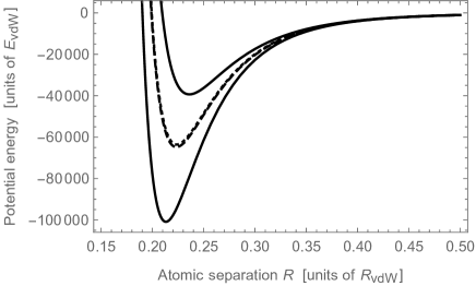
Figure 1: Adiabatic and diabatic potentials of the two-channel model. The solid curves represent the potentials $V_{-}$ and $V_{+}$ of Eqs. (97-98) for $\sigma_{-}=0.196\,R_{\text{vdW}}$, $\sigma_{+}=0.200\,R_{\text{vdW}}$, and $\delta=0$. For a weak adiabatic coupling strength $W=0.01$, the diabatic potentials $V_{\text{oo}}$ and $V_{\text{cc}}$ nearly coincide with the potentials $V_{+}$ and $V_{-}$. For a stronger adiabatic coupling strength $W=0.39$, the diabatic potentials $V_{\text{oo}}$ and $V_{\text{cc}}$ , shown by dashed and dotted curves, are nearly equal at short distance to the average of the two adiabatic potentials $V_{-}$ and $V_{+}$.

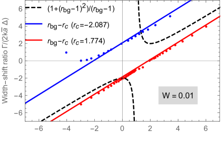
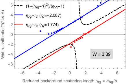
Figure 2: Ratio between the width parameter $\Gamma_{0}=\lim_{k\to 0}\Gamma/2k\bar{a}$ and shift $\Delta$, for resonances with different values of the reduced background scattering length $r_{\text{bg}}$ obtained by varying the short-range parameter $\sigma_{-}$ of the open-channel adiabatic potential $V_{-}$. The upper panel is obtained for a coupling strength $W=0.01$ for which the diabatic potentials are almost equal to the adiabatic potentials $V_{+}$ and $V_{-}$, and the lower panel is obtained for a coupling strength $W=0.39$ for which the diabatic potentials are nearly degenerate.

Changing $\sigma_{-}$ or $\sigma_{+}$ enables one to independently control the scattering lengths $a_{\text{o}}$ and $a_{\text{c}}$, as well as the positions of the bare energy levels of each adiabatic potential $V_{-}$ or $V_{+}$ . These quantities are easily obtained numerically using either a propagation method or a matrix representation with finite differences. To solve the two coupled equations, we first return to the original diabatic basis by using the transformation matrix $P$ of Eq. (104) and then solve the coupled equations (2-3) numerically. We can obtain the scattering length $a$ as a function of the energy separation $\delta$, which exhibits divergences that can be fitted by the formula $a=a_{\text{bg}}-\Gamma_{0}\bar{a}/(\delta-E_{0}).$ Comparing with Eq. (17), we obtain the width of the corresponding resonance $\lim_{k\to 0}\frac{\Gamma}{2k\bar{a}}=\Gamma_{0}$ and its shift $\Delta=E_{b}-E_{0}$, where $E_{b}$ is the binding energy of the closest molecular level (of energy $E_{m}=\delta-E_{b}$) in the closed-channel adiabatic potential $V_{+}$. We repeat this procedure for different values of $a_{\text{o}}$ that produce different values of $\Gamma_{0}$, $\Delta$ and $a_{\text{bg}}$. It is then possible to plot the ratio $\Gamma_{0}/\Delta$ as a function of $a_{\text{bg}}$. The result is shown in Fig. 2, for two different fixed values $a_{\text{c}}=-2.087\,R_{\text{vdW}}$ (blue points) and $a_{\text{c}}=1.774\,R_{\text{vdW}}$ (red points), and for two different values $W=0.01$ (upper panel) and $W=0.39$ (lower panel). The analytical formula of Eq. (49) predicts a linear behaviour that crosses zero at $a_{\text{bg}}=a_{\text{c}}$ (red and blue lines), which is verified to a large extent by the numerical data. In contrast, the formula of Eq. (50) does not depend on $a_{\text{c}}$ and predicts a qualitatively different behaviour (dashed curve) that is inconsistent with the numerical results.

We note that while the data for $W=0.01$ are well in the perturbative regime, as we find that $a_{\text{bg}}\approx a_{\text{o}}$ to a very good accuracy, the data for $W=0.39$ are at the limit of validity of the perturbative regime, because $a_{\text{bg}}$ is only approximately equal to $a_{\text{o}}$ and in a smaller range of values. Nevertheless, within that range, the formula of Eq. (49) appears to remain verified even at this coupling strength.

8 Application to lithium-6

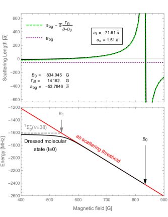
Figure 3: Broad Fano-Feshbach resonance of lithium-6 atoms in the hyperfine states ${a}$ and ${b}$ (first and second lowest states) around a magnetic field intensity of 834 G. Upper panel: s-wave scattering length as a function of the magnetic field intensity. Lower panel: energy spectrum (below the $ab$ scattering threshold) as a function of the magnetic field intensity. The solid black curve represents the energy of the dressed molecular state (with total nuclear spin ${I=0}$) associated with the broad resonance. The black arrow shows the resonance position $B_{0}$ at which the dressed molecular state reaches the threshold. The dashed grey line shows the energy of the last level of the singlet ${}^{1}\Sigma_{g}^{+}$ potential corresponding to the bare molecular state causing the resonance, intersecting the threshold at the bare resonance position $B_{1}$. Lengths are expressed in units of ${\bar{a}=1.5814}$ nm.

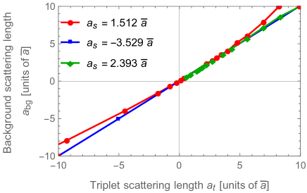
Figure 4: Background scattering length ${a_{{\rm bg}}}$ of the lithium-6 resonance as a function of the triplet scattering length ${a_{{\rm t}}}$, for different values of the singlet scattering length ${a_{{\rm s}}}$. This graph shows that ${a_{{\rm bg}}}$ is nearly independent of ${a_{{\rm s}}}$ and is approximately equal to ${a_{{\rm t}}}$. Lengths are expressed in units of ${\bar{a}=1.5814}$ nm.

Although we were able in the previous section to check our formula, Eq. (49), by numerically solving the two-channel equations (2-3) with van der Waals potentials, it is more difficult to verify that formula from experimental data or even from a realistic multi-channel calculation. While the width and background scattering lengths can usually be determined both experimentally and theoretically, the shift from the bare molecular state is more ambiguous, because it is not directly observable if the coupling causing the resonance cannot be tuned, as is the case for conventional magnetic Fano-Feshbach resonances.

Here, we consider the case of the broad resonance of lithium-6 atoms in the two lowest hyperfine states near a magnetic field intensity of 834 G, for which the bare molecular state causing the resonance has been identified as the last vibrational level of the singlet potential [26, 15]. This is illustrated in Fig. 3, which was obtained from a realistic multi-channel calculation taking into account the five relevant hyperfine channels. The upper panel shows that the variation of the scattering length is well fitted by the formula ${a=a_{{\rm bg}}-\bar{a}\Gamma_{B}/(B-B_{0})}$, making it possible to determine the “magnetic width” of the resonance ${\Gamma_{B}=14162}$ G, the resonance position ${B_{0}=834.045}$ G, and the background scattering length ${a_{{\rm bg}}=-53.78\,\bar{a}}$, where ${\bar{a}=1.5814}$ nm. The lower panel of Fig. 3 shows the molecular energy, which reaches the threshold at the resonance point ${B_{0}}$ (solid black curve, corresponding to a molecular state with total nuclear spin ${I=0}$) and the energy $E_{m}$ of the bare molecular state causing the resonance (dashed black line, corresponding to the last level $\nu=38$ of the singlet potential), which reaches the threshold at the magnetic field intensity $B_{1}=541.28$ G.

Comparing with Eq. (17), one finds

$$\delta\mu\,\Gamma_{B}=\lim_{k\to 0}\frac{\Gamma}{2k\bar{a}}\quad;\quad\delta\mu(B_{1}-B_{0})=\lim_{k\to 0}\Delta,$$ (99)

where ${\delta\mu}$ is the difference of magnetic moments between the bare molecule and the separated atoms. One can then calculate the ratio of the two quantities in Eq. (99):

$$\lim_{k\to 0}\frac{\Gamma}{2k\bar{a}\Delta}=\frac{\Gamma_{B}}{B_{1}-B_{0}}\approx-48.38$$ (100)

This value turns out to compare well with the value ${(1+(r_{{\rm bg}}-1)^{2})(r_{{\rm bg}}-1)^{-1}=-54.79}$ given by formula (50). However, as explained in the previous section, this is because the value of ${r_{{\rm bg}}}$ is unusually large, so that the formula reduces to ${\approx r_{{\rm bg}}=-53.79}$, which is also the limit of the formula given by Eq. (49). The broad 834 G resonance therefore does not allow one to discriminate between these formulas. For this purpose, one needs to theoretically change the value of the background scattering length.

It is not easy, in general, to control only the background scattering length by altering the Hamiltonian of the system. However, the case of lithium-6 is somewhat fortunate in that respect, because the background scattering length turns out to be given essentially by the the triplet scattering length ${a_{{\rm t}}}$ of the system, as shown in Fig. 4, while the closed channel is controlled by the singlet scattering length ${a_{{\rm s}}}$, since the close-channel bare molecular state is of a singlet nature. These values can be changed by slightly altering the shape of the triplet and singlet potentials at short distances.

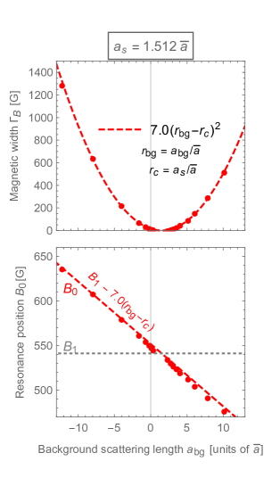
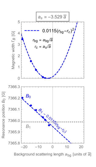
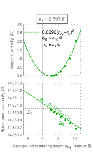
Figure 5: Plots of the magnetic width ${\Gamma_{B}}$ and position $B_{0}$ of the resonance [see Eqs. (99),(100) and discussion around] as a function of the reduced background scattering length ${r_{{\rm bg}}=a_{{\rm bg}}/\bar{a}}$, for three different singlet scattering lengths ${a_{{\rm s}}}$ indicated in the box at the top of each figure. The dots are obtained from a multi-channel calculation, while the dashed curves represent Eqs. (46) and (47).

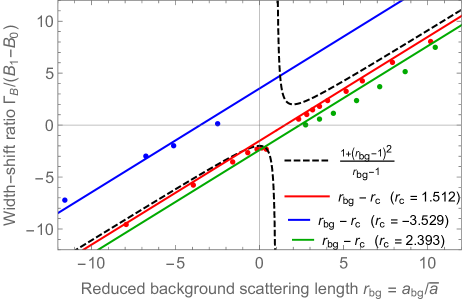
Figure 6: Ratio between the magnetic width $\Gamma_{B}$ and shift $B_{1}-B_{0}$, as a function of the reduced background scattering length $r_{\text{bg}}=a_{\text{bg}}/\bar{a}$, for different values of the reduced closed-channel scattering length $r_{{\rm c}}=a_{{\rm c}}/\bar{a}$. The dots are from a multi-channel calculation (see Fig. 5), and the solid lines correspond to Eq. (49), while the dashed curve corresponds to Eq. (50).

For fixed values of ${a_{{\rm s}}}$, we can extract and plot the magnetic width ${\Gamma_{B}}$ as a function of the background scattering length ${a_{{\rm bg}}}$, which is varied by varying ${a_{{\rm t}}}$. This is shown in the top panels of Fig. 5. Using the relation between the magnetic width and the energy width of the resonance in Eq. (99), the data can be well fitted by the adiabatic formula (46) where ${a_{{\rm c}}}$ is set to ${a_{{\rm s}}}$. This indicates that the resonance is in the adiabatic regime, and that the closed-channel molecular state is indeed controlled by the singlet scattering length ${a_{{\rm s}}}$, with $a_{{\rm c}}\approx a_{{\rm s}}$. A different value of ${\overline{\mathcal{W}}}$ has to be set for each value of ${a_{{\rm s}}}$ indicating that the coupling in the Hamiltonian is somehow modified when ${a_{{\rm s}}}$ is changed.

Next, for fixed values of ${a_{{\rm s}}}$, we can calculate the last singlet bound state energy, and find the magnetic field intensity $B_{1}$ at which the scattering threshold intersects that energy. In addition, we can extract the resonance position ${B_{0}}$ and plot it as a function of ${a_{{\rm bg}}}$. This is shown in the lower panels of Fig. 5. The resonance position ${B_{0}}$ varies approximately linearly with ${a_{{\rm bg}}}$ and intersects the value $B_{1}$ at $a_{\text{bg}}=a_{\text{c}}$, as expected from Eq. (47). Moreover, for each case, the slope of that linear dependence is consistent with the coefficient of the quadratic dependence of the width parameter, in agreement with Eqs. (46-47).

The ratio $\Gamma_{B}/(B_{1}-B_{0})$ of Eq. (100) is plotted in Fig. 6 as a function of the background scattering length $a_{\text{bg}}$. The linear variation of Eq. (49) is again validated and the explicit dependence of the results on the closed-channel scattering length ${a_{{\rm c}}}$ confirms the inadequacy of Eq. (50), which only depends on the background scattering length ${a_{{\rm bg}}}$. Although the results presented here support the validity of Eqs. (46-49), a full confirmation of these equations in the multi-channel case will be possible when a reliable way of determining the effective underlying two-channel model of a resonance is achieved, a task we leave as a future challenge.

9 Conclusion

This work has clarified the relationship between the width and shift of Fano-Feshbach resonances for van der Waals interactions. This insight will be crucial for the construction of effective interactions that can be used to treat few- or many-body problems, while faithfully reproducing the physics of Fano-Feshbach resonances. Experimentally, the determination of the shift is possible, as demonstrated recently [28]. The proposal in Ref. [29] for experimentally modifying the background scattering length of a given resonance is also a promising direction. This opens interesting perspectives to confirm our result. A similar analysis of the width and shift could also be of importance for resonances whose coupling can be controlled, such as microwave Fano-Feshbach resonances [30].

 

Acknowledgments

The authors would like to thank Paul S. Julienne, Eite Tiesinga, Servaas Kokkelmans, and Maurice Raoult for helpful discussions. P. N. acknowledges support from the RIKEN Incentive Research Project and JSPS Grants-in-Aid for Scientific Research on Innovative Areas (No. JP18H05407).

Appendix 1

The two-channel Hamiltonian of Eqs. (2-3) is

$$H=\left(\begin{array}[]{cc}T&0\\ 0&T\end{array}\right)+V$$ (101)

where $T$ is the kinetic operator $T=-\frac{\hbar^{2}}{2\mu}\frac{d^{2}}{dR^{2}}$ and $V$ is the potential matrix $\left(\begin{array}[]{cc}V_{\text{oo}}&V_{\text{oc}}\\ V_{\text{co}}&V_{\text{cc}}\end{array}\right)$. This expression of the Hamiltonian corresponds to the diabatic basis, which is a convenient representation for weak coupling $V_{\text{oc}}$. In the strong-coupling limit, the criterion of Eq. (18) is not verified and this representation becomes inconvenient. Instead, we consider the adiabatic basis obtained by diagonalising the potential matrix,

$$V^{\prime}=P^{-1}VP=\left(\begin{array}[]{cc}V_{+}&0\\ 0&V_{-}\end{array}\right)$$ (102)

where

$$V_{\pm}=\frac{V_{\text{oo}}+V_{\text{cc}}}{2}\pm\sqrt{\frac{(V_{\text{oo}}-V_{\text{cc}})^{2}}{4}+|V_{\text{oc}}|^{2}}$$ (103)

Assuming that $V$ is real, the transformation matrix $P$ is given by

$$P=\left(\begin{array}[]{cc}\cos\frac{\theta}{2}&-\sin\frac{\theta}{2}\\ \sin\frac{\theta}{2}&\cos\frac{\theta}{2}\end{array}\right)\qquad\text{with}\quad\tan\theta=\frac{2V_{\text{oc}}}{V_{\text{oo}}-V_{\text{cc}}}$$ (104)

where $0<\theta<\pi$. Although the potential becomes diagonal in the adiabatic basis, the kinetic operator transforms as follows:

$$P^{-1}TP=\left(\begin{array}[]{cc}T+\frac{\hbar^{2}}{2\mu}Q^{2}&-\frac{\hbar^{2}}{2\mu}\left[\frac{dQ}{dR}+2Q\frac{d}{dR}\right]\\ \frac{\hbar^{2}}{2\mu}\left[\frac{dQ}{dR}+2Q\frac{d}{dR}\right]&T+\frac{\hbar^{2}}{2\mu}Q^{2}\end{array}\right)$$ (105)

where the terms $Q(R)=-\frac{1}{2}\frac{d\theta(R)}{dR}$ arise from the action of the derivative operator in $T$. This gives rise to new off-diagonal couplings called radial couplings.

For magnetic Fano-Feshbach resonances of alkali atoms, the function $Q(R)$ shows a peak that can be located in the van der Waals region [20].

Appendix 2

Calculation of ${Y_{ij}}$ –

From Eqs. (2-3) we have

$$\psi_{{\rm o}}(R) =A\times\hat{f}_{{\rm o}}(R)+\int_{0}^{\infty}dR^{\prime}{\hat{\mathcal{G}}}_{{\rm o}}^{E}(R,R^{\prime})V_{{\rm oc}}(R^{\prime})\psi_{{\rm c}}(R^{\prime})$$

$$\psi_{{\rm c}}(R) =B\times\hat{f}_{{\rm c}}(R)+\int_{0}^{\infty}dR^{\prime}{\hat{\mathcal{G}}}_{{\rm c}}^{E}(R,R^{\prime})V_{{\rm co}}(R^{\prime})\psi_{{\rm o}}(R^{\prime}),$$

where ${A}$ and ${B}$ are two numbers, and we have introduced the two Green’s function,

$$\hat{\mathcal{G}}_{i}^{E}(R,R^{\prime})=\frac{2\mu}{\hbar^{2}}\frac{1}{W[\hat{f}_{i},\hat{g}_{i}]}\begin{cases}\hat{f}_{i}(R)\hat{g}_{i}(R^{\prime})&\text{for }R<R^{\prime}\\ \hat{f}_{i}(R^{\prime})\hat{g}_{i}(R)&\text{for }R>R^{\prime}\end{cases}$$ (106)

satisfying the radial equation,

$$\left(-\frac{\hbar^{2}}{2\mu}\frac{d^{2}}{dR^{2}}+V_{ii}(R)-E\right){\hat{\mathcal{G}}}_{i}^{E}(R,R^{\prime})=-\delta(R-R^{\prime})$$ (107)

and the appropriate boundary condition ${{\mathcal{G}}_{i}^{E}(R,R^{\prime})\xrightarrow[R\to 0]{}0}$, since both ${\hat{f}_{i}}$ are regular at the origin. This gives

$$\psi_{{\rm o}}(R) =A\times\hat{f}_{{\rm o}}(R)+(\hat{f}_{{\rm o}}|\psi_{{\rm c}})_{<}\hat{g}_{{\rm o}}(R)+(g_{{\rm o}}|\psi_{{\rm c}})_{>}\hat{f}_{{\rm o}}(R)$$

$$\psi_{{\rm c}}(R) =B\times\hat{f}_{{\rm c}}(R)+(\hat{f}_{{\rm c}}|\psi_{{\rm o}})_{<}\hat{g}_{{\rm c}}(R)+(g_{{\rm c}}|\psi_{{\rm o}})_{>}\hat{f}_{{\rm c}}(R).$$

Therefore, for ${R>R_{{\rm free}}}$,

$$\psi_{{\rm o}}(R) \xrightarrow[R\gtrsim R_{{\rm free}}]{}A\times\hat{f}_{{\rm o}}(R)+(\hat{f}_{{\rm o}}|\psi_{{\rm c}})\hat{g}_{{\rm o}}(R)$$

$$\psi_{{\rm c}}(R) \xrightarrow[R\gtrsim R_{{\rm free}}]{}B\times\hat{f}_{{\rm c}}(R)+(\hat{f}_{{\rm c}}|\psi_{{\rm o}})\hat{g}_{{\rm c}}(R).$$

We find the two linearly independent solutions ${\psi^{(1)}}$ and ${\psi^{(2)}}$ for ${(A,B)=(1,0)}$ and ${(A,B)=(0,1)}$. For ${(A,B)=(1,0)}$, we get

$$Y_{{\rm oo}}=-(\hat{f}_{{\rm o}}|\psi_{{\rm c}}^{(1)})\quad;\quad Y_{{\rm co}}=-(\hat{f}_{{\rm c}}|\psi_{{\rm o}}^{(1)}),$$ (108)

and for ${(A,B)=(0,1)}$, we get

$$Y_{{\rm oc}}=-(\hat{f}_{{\rm o}}|\psi_{{\rm c}}^{(2)})\quad;\quad Y_{{\rm cc}}=-(\hat{f}_{{\rm c}}|\psi_{{\rm o}}^{(2)}).$$ (109)

Limit of weak coupling

In the limit of weak coupling, one can make the following approximations:

$$Y_{{\rm co}} =-(\hat{f}_{{\rm c}}|\psi_{{\rm o}}^{(1)})\approx-(\hat{f}_{{\rm c}}|\hat{f}_{{\rm o}})$$ (110)

$$\psi_{{\rm c}}^{(1)} =\hat{g}_{{\rm c}}(\hat{f}_{{\rm c}}|\psi_{{\rm o}}^{(1)})_{<}+\hat{f}_{{\rm c}}(g_{{\rm c}}|\psi_{{\rm o}}^{(1)})_{>}$$ (111)

$$\approx\hat{g}_{{\rm c}}(\hat{f}_{{\rm c}}|\hat{f}_{{\rm o}})_{<}+\hat{f}_{{\rm c}}(g_{{\rm c}}|\hat{f}_{{\rm o}})_{>}$$

and therefore,

$$Y_{{\rm oo}}=-(\hat{f}_{{\rm o}}|\psi_{{\rm c}}^{(1)})=-\Big{(}\hat{f}_{{\rm o}}\Big{|}\hat{g}_{{\rm c}}(\hat{f}_{{\rm c}}|\hat{f}_{{\rm o}})_{<}+\hat{f}_{{\rm c}}(g_{{\rm c}}|\hat{f}_{{\rm o}})_{>}\Big{)}.$$ (112)

Likewise,

$$Y_{{\rm oc}} =-(\hat{f}_{{\rm o}}|\psi_{{\rm c}}^{(2)})\approx-(\hat{f}_{{\rm o}}|\hat{f}_{{\rm c}})$$ (113)

$$\psi_{{\rm o}}^{(2)} =\hat{g}_{{\rm o}}(\hat{f}_{{\rm o}}|\psi_{{\rm c}})_{<}+\hat{f}_{{\rm o}}(g_{{\rm o}}|\psi_{{\rm c}})_{>}$$ (114)

$$\approx\hat{g}_{{\rm o}}(\hat{f}_{{\rm o}}|\hat{f}_{{\rm c}})_{<}+\hat{f}_{{\rm o}}(g_{{\rm o}}|\hat{f}_{{\rm c}})_{>}$$

and therefore,

$$Y_{{\rm cc}}=-(\hat{f}_{{\rm c}}|\psi_{{\rm o}}^{(2)})\approx-\Big{(}\hat{f}_{{\rm c}}\Big{|}\hat{g}_{{\rm o}}(\hat{f}_{{\rm o}}|\hat{f}_{{\rm c}})_{<}+\hat{f}_{{\rm o}}(g_{{\rm o}}|\hat{f}_{{\rm c}})_{>}\Big{)}.$$ (115)

Appendix 3

In this appendix, we establish the connection between the coefficient $\alpha$ of Eq. (77) and the normalisation of the bound-state wave function $\hat{f}_{m}$ of section 6. The exponentially convergent function ${\psi_{{\rm c}}\approx\hat{f}_{{\rm c}}+\alpha(E-E_{m})\hat{g}_{{\rm c}}}$ becomes the closed-channel bound state ${\hat{f}_{m}}$ when $E=E_{m}$. The functions ${\psi_{{\rm c}}}$ and ${\hat{f}_{m}}$ are solutions of the closed-channel radial equations:

$$-\frac{\hbar^{2}}{2\mu}\psi_{{\rm c}}^{\prime\prime}+(V_{{\rm cc}}-E)\psi_{{\rm c}}=0$$ (116)

$$-\frac{\hbar^{2}}{2\mu}\hat{f}_{m}^{\prime\prime}+(V_{{\rm cc}}-E_{m})\hat{f}_{m}=0.$$ (117)

Multiplying the first equation by ${\hat{f}_{m}}$ and the second equation by ${\psi_{{\rm c}}}$, taking the difference between the two equations, and integrating gives

$$-\frac{\hbar^{2}}{2\mu}\int_{0}^{\infty}\left(\psi_{{\rm c}}^{\prime\prime}\hat{f}_{m}-\hat{f}_{m}^{\prime\prime}\psi_{{\rm c}}\right)dR\\ -(E-E_{m})\int_{0}^{\infty}\psi_{{\rm c}}\hat{f}_{m}dR=0.$$ (118)

Integrating by parts gives

$$\frac{\hbar^{2}}{2\mu}\left[\psi_{{\rm c}}^{\prime}\hat{f}_{m}-\hat{f}_{m}^{\prime}\psi_{{\rm c}}\right]_{R=0}-(E-E_{m})\int_{0}^{\infty}\psi_{{\rm c}}\hat{f}_{m}dR=0.$$ (119)

Using the explicit form of ${\psi_{{\rm c}}}$,

$$\frac{\hbar^{2}}{2\mu}\left[(\hat{f}_{{\rm c}}^{\prime}+\alpha(E-E_{m})\hat{g}_{{\rm c}}^{\prime})\hat{f}_{m}-\hat{f}_{m}^{\prime}(\hat{f}_{{\rm c}}+\alpha(E-E_{m})\hat{g}_{{\rm c}})\right]_{R=0}$$

$$-(E-E_{m})\int_{0}^{\infty}(\hat{f}_{{\rm c}}+\alpha(E-E_{m})\hat{g}_{{\rm c}})\hat{f}_{m}dR=0.$$ (120)

Using the fact that ${\hat{f}_{m}(0)=0}$ and ${\hat{f}_{{\rm c}}(0)=0}$, we obtain

$$\int_{0}^{\infty}(\hat{f}_{{\rm c}}+\alpha(E-E_{m})\hat{g}_{{\rm c}})\hat{f}_{m}dR=\frac{\hbar^{2}}{2\mu}\alpha W[\hat{f}_{m},\hat{g}_{{\rm c}}].$$ (121)

Finally, taking the limit ${E\to E_{m}}$, we get ${\hat{f}_{{\rm c}}\to\hat{f}_{m}}$, and ${W[\hat{f}_{m},\hat{g}_{{\rm c}}]\to W[\hat{f}_{m},\hat{g}_{m}]=1}$, which gives

$$\int_{0}^{\infty}\hat{f}_{m}^{2}dR=\frac{\hbar^{2}}{2\mu}\alpha.$$ (122)

This last equation relates the coefficient ${\alpha}$ to the normalisation of the bound state wave function ${\hat{f}_{m}}$. Thus, for ${E\approx E_{m}}$, the state ${\Psi_{{\rm c}}(R)=\frac{\hat{f}_{{\rm c}}(R)}{R}\sqrt{\frac{2\mu}{4\pi\hbar^{2}\alpha}}}$ is approximately the bound state ${\Psi_{m}(R)=\frac{\hat{f}_{m}(R)}{R}\sqrt{\frac{2\mu}{4\pi\hbar^{2}\alpha}}}$, with the proper normalisation ${\int_{0}^{\infty}4\pi R^{2}dR|\Psi_{m}(R)|^{2}=1}$.

References

- [1] H. Feshbach, “Unified theory of nuclear reactions” Annals of Physics, 5, 357 – 390, 1958.
- [2] U. Fano, “Effects of Configuration Interaction on Intensities and Phase Shifts” Phys. Rev., 124, 1866–1878, Dec 1961.
- [3] B. Verhaar, K. Gibble, and S. Chu, “Cold-collision properties derived from frequency shifts in a cesium fountain” Phys. Rev. A, 48, R3429–R3432, Nov 1993.
- [4] E. Tiesinga, B. J. Verhaar, and H. T. C. Stoof, “Threshold and resonance phenomena in ultracold ground-state collisions” Phys. Rev. A, 47, 4114–4122, May 1993.
- [5] S. Inouye, M. R. Andrews, J. Stenger, H.-J. Miesner, D. M. Stamper-Kurn, and W. Ketterle, “Observation of Feshbach resonances in a Bose-Einstein condensate” Nature, 392, 151–154, March 1998.
- [6] K. M. O’Hara, S. L. Hemmer, M. E. Gehm, S. R. Granade, and J. E. Thomas, “Observation of a Strongly Interacting Degenerate Fermi Gas of Atoms” Science, 298, 2179–2182, 2002.
- [7] C. A. Regal, C. Ticknor, J. L. Bohn, and D. S. Jin, “Creation of ultracold molecules from a Fermi gas of atoms” Nature, 424, 47–50, 2003.
- [8] T. Bourdel, L. Khaykovich, J. Cubizolles, J. Zhang, F. Chevy, M. Teichmann, L. Tarruell, S. J. J. M. F. Kokkelmans, and C. Salomon, “Experimental Study of the BEC-BCS Crossover Region in Lithium 6” Phys. Rev. Lett., 93, 050401, Jul 2004.
- [9] T. Kraemer, M. Mark, P. Waldburger, J. G. Danzl, C. Chin, B. Engeser, A. D. Lange, K. Pilch, A. Jaakkola, H.-C. Nägerl, and R. Grimm, “Evidence for Efimov quantum states in an ultracold gas of caesium atoms” Nature, 440, 315–318, 2006.
- [10] E. Haller, M. Gustavsson, M. J. Mark, J. G. Danzl, R. Hart, G. Pupillo, and H.-C. Nägerl, “Realization of an Excited, Strongly Correlated Quantum Gas Phase” Science, 325, 1224–1227, 2009.
- [11] A. Schirotzek, C.-H. Wu, A. Sommer, and M. W. Zwierlein, “Observation of Fermi Polarons in a Tunable Fermi Liquid of Ultracold Atoms” Phys. Rev. Lett., 102, 230402, Jun 2009.
- [12] P. Makotyn, C. E. Klauss, D. L. Goldberger, E. A. Cornell, and D. S. Jin, “Universal dynamics of a degenerate unitary Bose gas” Nat. Phys., 10, 116–119, Feb 2014.
- [13] M.-G. Hu, M. J. Van de Graaff, D. Kedar, J. P. Corson, E. A. Cornell, and D. S. Jin, “Bose Polarons in the Strongly Interacting Regime” Phys. Rev. Lett., 117, 055301, Jul 2016.
- [14] C. J. Joachain, Quantum Collision Theory, 3rd ed. North Holland, Amsterdam, 1983.
- [15] C. Chin, R. Grimm, P. Julienne, and E. Tiesinga, “Feshbach resonances in ultracold gases” Rev. Mod. Phys., 82, 1225–1286, Apr 2010.
- [16] E. Timmermans, P. Tommasini, M. Hussein, and A. Kerman, “Feshbach resonances in atomic Bose-Einstein condensates” Physics Reports, 315, 199–230, 1999.
- [17] C. Cohen-Tannoudji, “Atom-atom interactions in ultracold gases” DEA lecture at Institut Henri Poincaré, CEL online archive at https://cel.archives-ouvertes.fr/cel-00346023, 2007.
- [18] G. F. Gribakin and V. V. Flambaum, “Calculation of the scattering length in atomic collisions using the semiclassical approximation” Phys. Rev. A, 48, 546–553, Jul 1993.
- [19] J. L. Bohn and P. S. Julienne, “Semianalytic theory of laser-assisted resonant cold collisions” Phys. Rev. A, 60, 414–425, Jul 1999.
- [20] F. H. Mies, C. J. Williams, P. S. Julienne, and M. Krauss, “Estimating Bounds on Collisional Relaxation Rates of Spin-Polarized 87Rb Atoms at Ultracold Temperatures” J. Res. Natl. Inst. Stand. Technol., 101, 521, 1996.
- [21] T. G. Tiecke, M. R. Goosen, J. T. M. Walraven, and S. J. J. M. F. Kokkelmans, “Asymptotic-bound-state model for Feshbach resonances” Phys. Rev. A, 82, 042712, Oct 2010.
- [22] S. Kokkelmans Quantum gas experiments - exploring many-body states. Imperial College Press, London, 2014, ch. 4 - Feshbach Resonances in Ultracold Gases, 63–85, .
- [23] K. Góral, T. Köhler, S. A. Gardiner, E. Tiesinga, and P. S. Julienne, “Adiabatic association of ultracold molecules via magnetic-field tunable interactions” Journal of Physics B: Atomic, Molecular and Optical Physics, 37, 3457, 2004.
- [24] F. H. Mies, “A multichannel quantum defect analysis of diatomic predissociation and inelastic atomic scattering” J. Chem. Phys., 80, 2514, 1984.
- [25] B. P. Ruzic, C. H. Greene, and J. L. Bohn, “Quantum defect theory for high-partial-wave cold collisions” Phys. Rev. A, 87, 032706, 2013.
- [26] S. Simonucci, P. Pieri, and G. C. Strinati, “Broad vs. narrow Fano-Feshbach resonances in the BCS-BEC crossover with trapped Fermi atoms” Europhysics Letters (EPL), 69, 713–718, mar 2005.
- [27] N. Nygaard, B. I. Schneider, and P. S. Julienne, “Two-channel -matrix analysis of magnetic-field-induced Feshbach resonances” Phys. Rev. A, 73, 042705, Apr 2006.
- [28] R. Thomas, M. Chilcott, E. Tiesinga, A. B. Deb, and N. Kjærgaard, “Observation of bound state self-interaction in a nano-eV atom collider” Nature Communications, 9, 4895, 2018.
- [29] B. Marcelis, B. Verhaar, and S. Kokkelmans, “Total Control over Ultracold Interactions via Electric and Magnetic Fields” Phys. Rev. Lett., 100, 153201, Apr 2008.
- [30] D. J. Papoular, G. V. Shlyapnikov, and J. Dalibard, “Microwave-induced Fano-Feshbach resonances” Phys. Rev. A, 81, 041603(R), Apr 2010.