Competition between spin-induced charge instabilities in underdoped cuprates

Abstract

We study the static charge correlation function in an one-band model on a square lattice. The Hamiltonian consist of effective hoppings of the electrons between the lattice sites and the Heisenberg Hamiltonian. Approximating the irreducible charge correlation function by a single bubble yields the ladder approximation for the charge correlation function. In this approximation one finds in general three charge instabilities, two of them are due to nesting, the third one is the flux phase instability. Since these instabilities cannot explain the experiments in hole-doped cuprates we have included in the irreducible charge correlation function also Aslamasov-Larkin (AL) diagrams where charge fluctuations interact with products of spin fluctuations. We then find at high temperatures a nematic or $d$-wave Pomeranchuk instability with a very small momentum. Its transition temperature decreases roughly linearly with doping in the underdoped region and vanishes near optimal doping. Decreasing the temperature further a secondary axial charge-density wave (CDW) instability appears with mainly $d$-wave symmetry and a wave vector somewhat larger than the distance between nearest neighbor hot spots. At still lower temperatures the diagonal flux phase instability emerges. A closer look shows that the AL diagrams enhance mainly axial and not diagonal charge fluctuations in our one-band model. This is the main reason why axial and not diagonal instabilities are the leading ones in agreement with experiment. The two instabilities due to nesting vanish already at very low temperatures and do not play any major role in the phase diagram. Remarkable is that the nematic and the axial CDW instabilities show a large reentrant behavior.

I introduction

Cuprate superconductors show besides superconductivity and antiferromagnetism phases with different modulations of the charge and spin density M. Vojta (2009) including nematic Fradkin et al. (2010) and liquid-crystal Kivelson et al. (1998) phases. The striped or spin-charge ordered state in La-based compounds is well known. Kivelson et al. (2003) More recently, x-ray scattering has shown the existence of incommensurate CDW states which, different from stripes, are not accompanied by spin order. These CDWs exist in several hole-doped cuprates, Wu et al. (2011); Ghiringhelli et al. (2012); Chang et al. (2012); Achkar et al. (2012); Blackburn et al. (2013); LeBoeuf et al. (2013); Blanco-Canosa et al. (2014); Comin et al. (2014); da Silva Neto et al. (2014); Hashimoto et al. (2014); Tabis et al. (2014); Gerber et al. (2015); Y. Y. Peng, M. Salluzzo, X. Sun, A. Ponti, D. Betto, A. M. Ferretti, F. Fumagalli, K. Kummer, M. LeTacon, X. J. Zhou, N. B. Brookes, L. Braicovich, and G. Ghiringhelli (2016); Tabis et al. (2017) and have many properties in common: a) The modulation vector of the CDW is axial and decreases monotonically with increasing doping in contrast to the incommensurability of the spin fluctuations. K. Yamada, C. H. Lee, K. Kurahashi, J. Wada, S. Wakimoto, S. Ueki, H. Kimura, Y. Endoh, S. Hosoya, G. Shirane, R. J. Birgeneau, M. Greven, M. A. Kastner, and Y. J. Kim (1998); Haug et al. (2010); M. Hücker, M. v. Zimmermann, G. D. Gu, Z. J. Xu, J. S. Wen, G. Xu, H. J. Kang, A. Zheludev, and J. M. Tranquada (2011) b) In usual CDWs the electron and hole are localized at the same site, only their amplitude varies throughout the crystal. In contrast to that the electron and hole in the above cuprates are less localized and form a bound state with an internal $d$-wave symmetry. Comin et al. (2014); M. H. Hamidian, S. D. Edkins, Chung Koo Kim, J. C. Davis, A. P. Mackenzie, H. Eisaki, S. Uchida, M. J. Lawler, E.-A. Kim, S. Sachdev, and K. Fujita (2016) c) The cross-over temperature $T_{{\rm CDW}}$ to this new CDW state lies well below the pseudogap temperature $T^{*}$ and shows a domelike shape Blanco-Canosa et al. (2014) as a function of doping. Near its maximum a nematic transition line increases rapidly with decreasing doping. Cyr-Choinière et al. (2018)

Theoretically it has been proposed that CDW instabilities, including nematic or $d$-wave Pomeranchuk instabilities, are caused either by the pseudogap phase Atkinson et al. (2015); Comin et al. (2014); Atkinson et al. (2016) and the related modification of the bandstructure or occur in the paramagnetic state due to antiferromagnetic exchange interactions. Yamase and Kohno (2000a, b); Cappelluti and Zeyher (1999); Halboth and Metzner (2000); Yamase and Metzner (2007); M. A. Metlitski and S. Sachdev (2010); Husemann and Metzner (2012); Bejas et al. (2012); Sachdev and LaPlaca (2013); Allais et al. (2014); Sau and Sachdev (2014); Efetov et al. (2013) In the second case mean-field calculations Cappelluti and Zeyher (1999); Bejas et al. (2012); Sachdev and LaPlaca (2013); Allais et al. (2014) yield a CDW instability to a flux state with a momentum near $(\pi,\pi)$ or an instability with a nesting vector connecting hot spots along the diagonals. These instabilities are diagonal and not axial as in the experiment. Calculations based on the spin fermion model found an instability with an axial wave vector connecting neighboring hot spots. Wang and Chubukov (2014) Whether the employed simple ladder diagrams can produce a CDW with an axial momentum is presently not clear. Mishra and Norman (2015) A spin fermion model with overlapping hot spots may, however, yield an axial CDW instability. P. A. Volkov and K. B. Efetov (2016)

A three-band Hubbard model treated in the mean-field approximation plus a charge interaction induced by product of spins (Aslamasov-Larkin or AL diagrams) yielded a CDW with the correct $d$-wave symmetry and a wave vector related to hot spots. Y. Yamakawa and H. Kontani (2015); Tsuchiizu et al. (2016) Whether this three band model can be applied to cuprates is unclear because the formation of Zhang-Rice singlets F.C. Zhang and T.M. Rice (1988) and the associated reduction of degrees of freedom is not taken into account. AL diagrams have been used in the past for calculating the effect of fluctuations on the conductivity, Aslamasov and Larkin (1968) on Raman scattering Caprara et al. (2015); Kampf and Brenig (1992) and phonon anomalies. Liu et al. (2016)

In this paper we study charge instabilities of the one-band $t$-$J$ model treating the constraint in the mean-field approximation. We also include Aslamasov-Larkin diagrams as a natural generalization of the ladder approximation. These diagrams produce two kinds of charge instabilities: nematic or $d$-wave Pomeranchuk instabilities with extremely small wave vectors as primary, and CDWs with internal $d$-wave symmetries and much larger wave vectors as secondary instabilities. Our approach uses Green’s and vertex functions on the real frequency axis which allows to treat both low and high temperatures. We address, in particular, the following points which presently are not well understood: Why is the axial and not the diagonal charge instability seen in experiment? Is there more than one charge instability and what happens to the mean-field flux instability if the AL diagram is taken into account?

The paper is organized as follows. After an introduction in section I we specify the Hamiltonian in section II and discuss some of its properties which are relevant for the following. This section also contains a discussion of the diagrams taken into account in our calculation, namely, ladder and sums of ladder diagrams (details are given in Appendix A) and AL diagrams. The evaluation of these diagrams is given in section III. In section IV we investigate $d$-wave charge instabilities as a function of temperature and doping using only one basis function with $d$-wave symmetry to represent charge fluctuations. Since the evaluation of the AL diagrams is somewhat involved we present details of it in Appendix B. Finally, we consider in Appendix C a complete set of four basis functions for charge fluctuations and the related 4x4 susceptibility matrices. It is shown that the leading instability has indeed mainly $d$-wave symmetry. We also discuss the relationship between different definitions of $d$-wave charge susceptibilities and the set of employed basis functions.

II Hamiltonian and choice of diagrams

We consider the following effective Hamiltonian for electrons moving on a square lattice,

$$H= -\sum_{i,j,\alpha}\delta t_{ij}c^{\dagger}_{i\alpha}c_{j\alpha}$$

$$+\frac{J}{4}\sum_{{\langle i,j\rangle}\atop{\alpha,\beta}}(c^{\dagger}_{i\alpha}c_{i\beta}\;\;c^{\dagger}_{j\beta}c_{j\alpha}-c^{\dagger}_{i\alpha}c_{i\alpha}\;\;c^{\dagger}_{j\beta}c_{j\beta}).$$ (1)

$c_{i\alpha}^{\dagger}$ and $c_{i\alpha}$ are fermionic creation and annihilation operators for electrons on site $i$ and spin direction $\alpha$. $t_{ij}$ denote effective hopping amplitudes for electrons between the sites $i$ and $j$. The second term in Eq. (1) represents the Heisenberg interaction where $J$ is the Heisenberg constant and $\langle ij\rangle$ denotes nearest-neighbor sites $i$ and $j$. $\delta$ is the hole doping. Without the factor $\delta$ in the first term in Eq. (1) $H$ describes a $t$-$J$ model without any restrictions on double occupancies, see Ref. [Chowdhury and Sachdev, 2014]. The conventional $t$-$J$ model is obtained if a constraint is added to $H$ which excludes double occupancies of lattice sites.

The effective Hamiltonian Eq. (1) captures important features of the charge excitation spectrum of the $t$-$J$ model. The fermionic operators of the $t$-$J$ model act in the Fock space without double occupancies; they are Hubbard $X$-operators and not the usual creation and annihilation operators. In the large-$N$ limit based on $X$-operatorsZeyher and Kulić (1996); Greco and Zeyher (2006) the $t$-$J$ model becomes, however, equivalent to an effective Hamiltonian written in terms of usual creation and annihilation operators (see Eq.(12) in Ref.[Greco and Zeyher, 2006]). It contains a kinetic term where the hopping is renormalized by $\delta$ neglecting a small contribution proportional to $J$. A second term represents an effective interaction consisting of six separable channels. Channels $3$-$6$ represent the Heisenberg interaction, channels $1$-$2$ originate from the constraint. Channels $1$-$2$ may be neglected in our case because we are not interested in s-wave fluctuations and because one can show that they couple only weakly to the other channels, Ref.[Cappelluti and Zeyher, 1999]. The effective Hamiltonian Eq.(12) in Ref.[Greco and Zeyher, 2006] becomes then our Hamiltonian Eq. (1). The large-N treatment thus replaces the hard constraint at $N=2$ by the soft constraint at $N=\infty$. Calculating the density correlation function with X-operators in the limit $N$ to $\infty$ and dropping the channels 1 and 2 yields the same result as a calculation using Eq. (1) and a low-order ladder approximation. Many calculations of the spin susceptibility are based on $H$ of Eq. (1) using the random phase approximation for the Heisenberg interaction and a renormalized hopping term, see Refs.[Brinckmann and Lee, 1999; Norman, 2001].

It is convenient to rewrite $H$ in momentum space. The first term in the parenthesis in $H$ becomes,

$$H_{J}=-\frac{1}{4}\sum_{{{\bf p^{\prime}}{\bf p^{\prime\prime}}{\bf k}}\atop{\alpha,\beta}}J({\bf p^{\prime}}-{\bf p^{\prime\prime}})c^{\dagger}_{{\bf p^{\prime}}+{\bf k},\alpha}c_{{\bf p^{\prime}},\alpha}c^{\dagger}_{{\bf p^{\prime\prime}},\beta}c_{{\bf p^{\prime\prime}}+{\bf k},\beta}$$ (2)

with $J({\bf p})=2J(\cos(p_{x})+\cos(p_{y}))$. $J({\bf p^{\prime}}-{\bf p^{\prime\prime}})$ can be written as a sum over 4 separable kernels,

$$J({\bf p^{\prime}}-{\bf p^{\prime\prime}})=4J\sum_{r=1}^{4}\gamma_{r}({\bf p^{\prime}})\gamma_{r}({\bf p^{\prime\prime}}).$$ (3)

The functions $\gamma_{r}({\bf p})$ are given by $\gamma_{1}({\bf p})=(\cos(p_{x})-\cos(p_{y}))/2$, $\gamma_{2}({\bf p})=(\cos(p_{x})+\cos(p_{y}))/2$, $\gamma_{3}({\bf p})=(\sin(p_{x})-\sin(p_{y}))/2$, $\gamma_{4}({\bf p})=(\sin(p_{x})+\sin(p_{y}))/2$. Using the charge variables

$$n_{r}({\bf k})=\sum_{{\bf p},\alpha}\gamma_{r}({\bf p})c^{\dagger}_{{\bf p}+{\bf k},\alpha}c_{{\bf p},\alpha},$$ (4)

and inserting Eq. (3) into Eq. (2) yields

$$H_{J}=-J\sum_{{\bf k},r}n_{r}({\bf k})n^{\dagger}_{r}({\bf k}).$$ (5)

Using similar arguments the last term in $H$ is found to be equal to $-H_{J}/2$ neglecting small non-local spin interaction terms. Altogether the effective Hamiltonian $H$ becomes,

$$H=\sum_{{\bf k},\alpha}\epsilon_{\bf k}c^{\dagger}_{{\bf k},\alpha}c_{{\bf k},\alpha}+H^{\prime}.$$ (6)

$\epsilon_{\bf k}$ are one-particle energies,

$$\epsilon_{\bf k}=-2t{\delta}(\cos(k_{x})+\cos(k_{y}))-4t^{\prime}\delta\cos(k_{x})\cos(k_{y}),$$ (7)

$t$ and $t^{\prime}$ denote hopping amplitudes between nearest and second nearest neighbors, respectively. $H^{\prime}$ is the interaction part of $H$ given by

$$H^{\prime}=-\frac{J}{2}\sum_{r,{\bf k}}n_{r}({\bf k})n_{r}^{\dagger}({\bf k}).$$ (8)

The Matsubara Green’s function describing charge fluctuations reads

$$\Pi_{rs}({\bf k},\tau_{1}-\tau_{2})=-\langle{\cal T}(n_{r}^{\dagger}({\bf k},\tau_{1})n_{s}({\bf k},\tau_{2}))\rangle.$$ (9)

$\tau_{1}$ and $\tau_{2}$ are imaginary times, ${\cal T}$ the time ordering operator and $\langle...\rangle$ the expectation value. $\Pi_{rs}$ is a 4x4 matrix describing the coupling of charge fluctuations with the symmetries $r$ and $s$. After a Fourier transform with respect to $\tau_{1}-\tau_{2}$, $\Pi$ can be written as $\Pi(k)$ where $k$ denotes both the momentum $\bf k$ and the Matsubara frequency ${\rm i}\omega_{n}$, $k=({\bf k},{\rm i}\omega_{n})$. Using $H^{\prime}$ and performing a sum over ladders one obtains

$$\Pi_{rs}(k)= \Pi^{(0)}_{rs}(k)-\sum_{t}\Pi^{(0)}_{rt}(k)J\Pi^{(0)}_{ts}(k)+...$$

$$= \sum_{t}\Pi^{(0)}_{rt}(1+J\Pi^{(0)}(k))^{-1}_{ts}.$$ (10)

Eq. (10) is derived in Appendix A for the simplest case where $\Pi^{(0)}_{rs}(k)$ is given by the unperturbed charge Green’s function, i.e., by a simple fermionic bubble. More generally, $\Pi^{(0)}_{rs}(k)$ denotes the irreducible part of the charge Green’s function which consists of all diagrams of $\Pi_{rs}(k)$ which cannot be written as a matrix product of the $\Pi_{uv}^{(0)}(k)$ times powers of $J$. In Appendix C we show that fluctuations in the $d$-wave channel $r=1$ are much stronger than in the other three channels and mix only weakly with them. It is therefore admissible to limit ourselves in the main part of the paper to $r=s=1$ and to drop the index 1 altogether. For a different definition of the charge variables see last section of Appendix C.

The diagrams which we will take into account for $\Pi^{(0)}(k)$ are shown in Fig. 1. Solid lines represent unperturbed electronic Green’s functions. Small filled circles stand for the d-wave vertex $\gamma({\bf p})$, the wavy lines represent spin propagators. The physical meaning of the diagrams is rather clear. The first diagram describes the free propagation of charge excitations between two rungs of the ladder represented by the small filled circles. We denote it by $\Pi^{(0)}_{0}(k)$. In the second diagram the charge excitation transforms on the way between two rungs into a product of spin excitations and then back into a charge excitation. In this way two spin excitations can make an important contribution to charge correlation functions. Interchanging the two right ends of the spin propagators in the second diagram in Fig. 1 yields the third diagram where the spin propagators cross each other. This topologically inequivalent diagram has also to be taken into account. We will call the second and third diagrams Aslamasov-Larkin diagrams and denote their sum by $\Pi_{AL}^{(0)}(k)$. In the following we are interested in the static limit and put therefore the external frequency ${\rm i}\omega_{n}$ to zero. We also choose the hopping $t$ and the lattice constant $a$ as energy and length units, respectively, and put $J=0.28$ and $t^{\prime}=-0.3$ throughout the paper.

Figure 1: Bubble and Aslamasov-Larkin diagrams for $\Pi^{(0)}$.

In the present paper Maki-Thompson processes, as those considered in Ref.[Wang and Chubukov, 2014], are not included. In Ref. [Wang and Chubukov, 2014] an axial CDW was obtained, however, this result is controversialMishra and Norman (2015). The authors of Ref.[Mishra and Norman, 2015] find that these processes lead to a diagonal CDW. For this reason and because a proper calculation of the Maki-Thompson diagrams are beyond the scope of the present paper we focus on AL diagrams for an explanation for the observed axial CDW.

III Evaluation of the diagrams

The first diagram in Fig. 1 is the single bubble contribution to $\Pi^{(0)}(k)$ given by,

$$\Pi_{0}^{(0)}({\bf k})=-2\sum_{\bf p}\gamma^{2}({\bf p})\frac{f(\epsilon_{{\bf k}+{\bf p}}-\mu)-f(\epsilon_{\bf p}-\mu)}{-\epsilon_{{\bf k}+{\bf p}}+\epsilon_{\bf p}}.$$ (11)

$f(\epsilon)$ is the fermionic occupation number and $\mu$ the chemical potential. The solid and dotted lines in Fig. 2 show $\Pi_{0}^{(0)}({\bf k})$ for $T=0.00002$ and $T=0.01$, respectively. The doping is $\delta=0.11$ and the momentum $\bf k$ varies from $(0,0)$ to $(\pi,0)$ and $(\pi,\pi)$ and back to $(0,0)$. The horizontal, dotted line corresponds to $\Pi^{(0)}({\bf k})=-1/J$ where the denominator of Eq. (10) is zero and an instability of the normal state occurs. The solid line, describing the low-temperature case, exhibits two sharp dips at the momenta ${\bf k_{\rm 1}}=(0.832,0)$ and ${\bf k}_{\rm 4}=(0.988,0.988)$. As shown in the inset of Fig. 2 these momenta join nested regions along axial and diagonal directions, respectively. T. Holder and W. Metzner (2012) Dips due to nesting are extremely sensitive to temperature and vanish even at moderate temperatures as illustrated by the solid and dotted lines in Fig. 2. Figure 2 shows another dip which is rather broad and much less sensitive to temperature. Its wave vector ${\bf k}_{\rm 3}=(\pi,\pi)$ connects two more distant hot spots as shown in the inset of Fig. 2. The Fermi lines near these hot spots are not parallel to each other causing a rather broad and weakly temperature dependent $\Pi_{0}^{(0)}({\bf k})$ near ${\bf k}_{\rm 3}$. In spite of the absence of nesting this instability is rather robust and leads at low temperatures to the staggered flux state with circulating currents. Cappelluti and Zeyher (1999) Figure 2 shows that $\Pi_{0}^{(0)}$ is not able to account for the experimental findings in underdoped cuprates: Observed charge density waves in axial direction cannot be ascribed to the low-temperature dip at ${\bf k}_{1}$ and the predicted flux state in diagonal direction is not seen in the experiment. The wave vector ${\bf k}_{2}$ connecting nearest neighbor hot spots in vertical or horizontal direction does not cause any dip in $\Pi_{0}^{(0)}({\bf k})$ though it is near to the wave vector of the experimentally observed charge order. We therefore propose that higher-order terms to $\Pi^{(0)}({\bf k})$ such as the AL diagrams should be included.

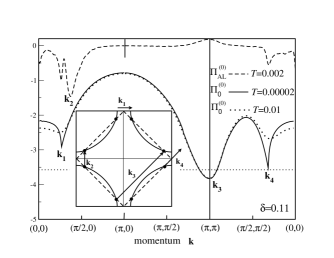
Figure 2: (color online) Momentum dependence of $\Pi_{0}^{(0)}({\bf k})$ and $\Pi_{AL}^{(0)}({\bf k})$ for doping $\delta=0.11$. ${\bf k}_{1}$ - ${\bf k}_{4}$ denote nesting vectors or vectors connecting hot spots, the latter are shown as filled circles in the inset.

The calculation of the second and third diagrams, the AL diagrams, needs some care in performing the analytic continuation. The usual procedure to sum over pole contributions leads in general to Green’s functions which should be evaluated right on the cut. Clearly, the resulting singularities must vanish again if all pole contributions are taken into account. Since it is difficult to achieve such a compensation explicitly we describe in detail a method in Appendix B where the compensation is done analytically. Our final result for the AL diagrams is,

$$\Pi_{AL}^{(0)}({\bf k}) =-\frac{3}{8\pi}\sum_{\bf q}J^{2}({\bf q})J^{2}({\bf k}-{\bf q})\int d\epsilon\;n(\epsilon)\Big{\{}$$

$$[{\rm Im}D({\bf q},\epsilon){\rm Re}D({\bf k}-{\bf q},-\epsilon)$$

$$+{\rm Re}D({\bf q},\epsilon){\rm Im}D({\bf k}-{\bf q},\epsilon)]$$

$$\times[({\rm Re}V^{S}({\bf k},{\bf q},\epsilon))^{2}-({\rm Im}V^{S}({\bf k},{\bf q},\epsilon))^{2}]$$

$$+2{\rm Im}V^{S}({\bf k},{\bf q},\epsilon){\rm Re}V^{S}({\bf k},{\bf q},\epsilon)$$

$$\times[{\rm Re}D({\bf q},\epsilon){\rm Re}D({\bf k}-{\bf q},\epsilon)$$

$$-{\rm Im}D({\bf q},\epsilon){\rm Im}D({\bf k}-{\bf q},\epsilon)]\Big{\}}.\;\;\;$$ (12)

$n(\epsilon)$ is equal to $1/({\rm exp}(\epsilon/T)-1)$ and $V^{S}$ is the symmetrized vertex given by

$$V^{S}({\bf k};{\bf q},\epsilon)= V({\bf k};{\bf q},\epsilon)+{\tilde{V}}({-\bf k};{-\bf q},-\epsilon),$$ (13)

with

$$V(k;q)=T\sum_{p}\gamma({\bf p})G(p)G(p+k)G(p+q),$$ (14)

$${\tilde{V}}(k;q)=T\sum_{p}\gamma({\bf p})G(p)G(p+k)G(p+k-q).$$ (15)

An explicit expression for $V(k;q)$ is given in Eq. (20).

Using the symmetrized vertex $V^{S}$ both AL diagrams are taken into account. $D({\bf k},\epsilon)$ is the spin response function given in Refs. Sherman, 2004; A.A. Vladimirov, D. Ihle, and N.M. Plakida, 2009; Tacon et al., 2011

$$D({\bf k},\epsilon)=\frac{A(1-\gamma_{\bf k})}{\omega_{\bf k}^{2}-\epsilon^{2}-{\rm i}\Gamma\epsilon},$$ (16)

with $\gamma_{\bf k}=(\cos(k_{x})+\cos(k_{y}))/2$, $\omega_{\bf k}^{2}=4J^{2}(1-\gamma_{\bf k})(1+\gamma_{\bf k}+1/(4\xi^{2}))$. $\xi$ is the magnetic correlation length given approximately by $\xi^{2}=1.6/\delta$, A.A. Vladimirov, D. Ihle, and N.M. Plakida (2009) $\Gamma$ is a phenomenological damping chosen to be 0.6 and $A$ a constant to be determined from the spin sum rule. Equation (16) describes well the experimental spin correlation function over a large doping region and represents a simplified version of the theoretically derived expressions in Refs. Sherman, 2004; A.A. Vladimirov, D. Ihle, and N.M. Plakida, 2009. For the numerical evaluation of the momentum sums in Eqs. (12), (14) and (15) we used 50x50 or 100x100 nets in the Brillouin zone, for the integration over $\epsilon$ in Eq. (12) about 1200 points.

The dashed curve in Fig. 2 shows the momentum dependence of $\Pi_{AL}^{(0)}$ at low temperature $T=0.002$. $\Pi_{AL}^{(0)}({\bf k})$ is over a wide momentum region small compared to $\Pi_{0}^{(0)}({\bf k})$, especially along the directions $(\pi,0)$ - $(\pi,\pi)$ - $(0,0)$. The smallness of $\Pi_{AL}^{(0)}({\bf k})$ along the diagonal can be understood in the following way: The main contribution in the sum over $\bf q$ in Eq. (12) comes from the region ${\bf q}\approx{\bf Q}=(\pi,\pi)$ and $\approx{\bf Q}-{\bf k}$ if $\xi$ is much larger than 1. $\bf q$ may then be fixed in $V^{S}({\bf k},{\bf q},\epsilon)$ to these values. Applying a reflection along the diagonal to the vertices $V$ and $\tilde{V}$ in Eqs. (14) and (15) reproduces $V$ and $\tilde{V}$ except for a minus sign due to the form factor $\gamma({\bf p})$. As a result $V$, $\tilde{V}$ and thus also $V^{S}$ and $\Pi_{AL}^{(0)}$ are zero if ${\bf k}$ lies along the diagonal. Allowing for the momentum dependence of the vertices $\Pi_{AL}^{(0)}({\bf k})$ is not exactly zero there but still small. As a result diagonal instabilities are not much enhanced by the AL diagram in our one-band model. This is different from the three-band model of Refs. Y. Yamakawa and H. Kontani, 2015; Tsuchiizu et al., 2016 where the AL diagram enhances both axial and diagonal charge fluctuations. The biggest modification of $\Pi_{0}^{(0)}$ by the AL diagram occurs in the axial direction between $(0,0)$ and $(\pi/2,0)$. Both $\Pi_{0}^{(0)}$ and $\Pi_{AL}^{(0)}$ show dips near the nesting vector ${\bf k}_{1}$. However, there is an additional dip in $\Pi_{AL}^{(0)}$ which is present only in $\Pi_{AL}^{(0)}$ and occurs at ${\bf k}_{{\rm min}}$ near the vector ${\bf k}_{2}$ (see the inset in Fig. 2) which connects nearest neighbor hot spots in the vertical or horizontal direction.

IV Charge instabilities

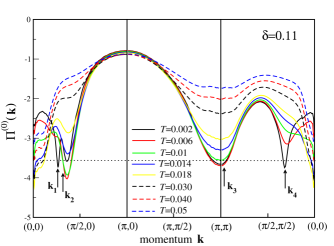
Figure 3: (color online) Momentum dependence of $\Pi^{(0)}({\bf k})$ for different temperatures and $\delta$ = 0.11.

The total irreducible charge correlation function is given by

$$\Pi^{(0)}({\bf k})=\Pi_{0}^{(0)}({\bf k})+\Pi_{AL}^{(0)}({\bf k}).$$ (17)

Figure 3 shows the momentum dependence of $\Pi^{(0)}({\bf k})$ throughout the Brillouin zone for 8 different temperatures. Disregarding the axial direction and the region very close to $\Gamma$ there are two minima near the momenta ${\bf k}_{\rm 3}$ and ${\bf k}_{\rm 4}$ which were present already in $\Pi_{0}^{(0)}$, see Fig. 2. The minimum with momentum ${\bf k}_{\rm 4}$ is due to nesting, shifts rapidly upwards with increasing temperature and soon ceases to be even a local minimum. The minimum with momentum ${\bf k}_{3}$ is broad, moves first with increasing temperature a little downwards and then slowly upwards. It does not change much its shape and remains a local minimum at all temperatures shown. Figure 4 shows the same curves as in Fig. 3 but in the small interval between $(0,0)$ and $(2,0)$. The minimum of $\Pi^{(0)}({\bf k})$ located near ${\bf k}_{\rm 1}$ is extremely sensitive to temperature and exists no longer above $T=0.006$. There is another minimum in axial direction at ${\bf k}_{{\rm min}}$, see Fig. 4. Its doping dependence and its closeness to ${\bf k}_{\rm 2}$ (see the inset of Fig. 6) suggest that it originates from transitions between nearest neighbor hot spots. Since in this case the nesting is only approximate the transitions involve a large region of momentum states around the hot spots. As a result ${\bf k}_{{\rm min}}$ deviates substantially from ${\bf k}_{\rm 2}$ and the temperature dependence around ${\bf k}_{{\rm min}}$ is rather weak similar as in the case of the flux state dip near ${\bf k}_{\rm 3}$. $\Pi^{(0)}({\bf k}_{{\rm min}})$ lies very near to the normal state at low temperatures, decreases first substantially with increasing temperature and then increases and moves back into the normal state. A similar reentrant behavior is found for $\Pi^{(0)}({\bf k})$ at small k near ${\bf k}=(0.03,0)$, see Fig. 4. It exhibits a minimum which moves first down from the normal state deep into the unstable region, reaches there an absolute minimum and then moves upwards again into the normal state. Interesting is that the relative or absolute minimum of $\Pi^{(0)}({\bf k})$ never occurs exactly at ${\bf k}=0$. This means that the homogeneous state is unstable against a modulation with a perhaps small, but finite wave vector ${\bf k}$.

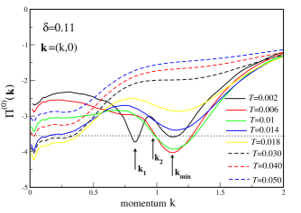
Figure 4: (color online) Enlarged Fig. 3 for axial momenta between $(0,0)$ and $(2,0)$.

The transition temperatures for charge modulations were obtained by starting at high temperatures and then lowering the temperature until minima of $\Pi^{(0)}({\bf k})$ cross the dotted line at $-1/J\sim-3.57$. The first crossing occurs at a very small momentum ${\bf k}\approx(0.03,0)$ and a temperature of about $T_{{\rm nem}}\sim 0.04$ and describes the transition to a nematic state. Due to the reentrant behavior of $\Pi^{(0)}$ there is another crossing at around $T\sim 0.011$ from the nematic back to the normal state. Lowering further the temperature the dip near ${\bf k}_{{\rm min}}$ touches the dotted line at around $T_{{\rm CDW}}\sim 0.0128$ as can be seen in Fig. 4. Due to the reentrant behavior there is also in this case a second crossing of $\Pi^{(0)}$ at a very low temperature $T_{{\rm CDW}}\sim 0.001$ to the normal state. For the temperature $T=0.014$, $\Pi^{(0)}({\bf k})$ lies except for very small momenta everywhere above the critical line. This means that it is stable with respect to other CDW states, in particular, the flux state with momentum ${\bf k}_{\rm 3}$. The dips near the perfect nesting vectors ${\bf k_{\rm 1}}$ and ${\bf k}_{\rm 4}$ can lead to instabilities only at very low temperatures as can be seen from Figs. 3 and 4. At higher temperatures these dips no longer exist. Figs. 3 and 4 show that the CDW state forms in general in the presence of the nematic state. This means that the band stucture of the nematic state and not that of the normal state should be used in calculating the CDW instabilities. Below we will show that the nematic distortion enhances the CDW instabilities but that in a first approximation this effect may be neglected.

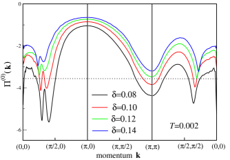
Figure 5: (color online) Momentum dependence of $\Pi^{(0)}({\bf k})$ at $T=0.002$ for different dopings.

Figure 5 shows the momentum dependence of $\Pi^{(0)}({\bf k})$ at a low temperature for different dopings. Interesting is that the axial minima outside of the nematic region are much lower than the diagonal ones for $\delta=0.08$. With increasing doping this difference becomes smaller. At around $\delta=0.12$ the lowest axial and diagonal dips have about the same depth. Increasing $\delta$ further the diagonal minima would be lower than the axial ones. However, all the minima would lie then above the dotted line and thus would not cause any instabilities.

The transition temperatures can be determined in the same way as in Fig. 4 for $\delta=0.11$. The result is shown in Fig. 6 by squares for the nematic and by circles for CDW states. Calculated transition temperatures have been smoothly joined by dashed curves and consist of two branches due to the reentrance behavior. Reentrant behavior has also been found previously in a model with forward scattering and BCS pairing interactions Yamase and Metzner (2007) and in the Hubbard model. R. Pietig, R. Bulla, and S. Blawid (1999) The modulated state exists in each case between the upper and lower branch. If no reentrance occurs the lower branch is given by the x-axis. Figure 6 indicates that in our approach nematic and CDW states are related and direct consequences of the AL diagrams. Compared with the experimental phase diagrams in Fig. 18 of Ref. Cyr-Choinière et al., 2018 and Fig. 3 of Ref. Y. Sato, S. Kasahara, H. Murayama, Y. Kasahara, E.-G. Moon, T. Nishizaki, T. Loew, J.Porra, B. Keimer, T. Shibauchi and Y. Matsuda, 2017 and disregarding the reentrant behavior essential features of the experiments are roughly reproduced. For instance, the strong, approximately linear decrease of $T_{{\rm nem}}$ with doping and the approach of $T_{{\rm nem}}$ to the weakly doping dependent $T_{{\rm CDW}}$ from above. The reentrant behavior has so far not been reported experimentally and is at present a theoretical prediction. The filled and empty circles in the inset of Fig. 6 show the doping dependence of the length of ${\bf k}_{2}$ and of ${\bf k}_{{\rm min}}$, respectively. The squares, triangles and diamonds are experimental data. The filled circles lie always a little below the empty circles. This means that in momentum space an extended region around the hot spots contributes to the CDW instability. This also explains the weak temperature dependence of $\Pi^{(0)}({\bf k})$ around ${\bf k}_{{\rm min}}$, compared to the regions around the minima near ${\bf k_{\rm 1}}$ and ${\bf k_{\rm 4}}$.

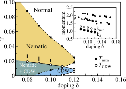
Figure 6: (color online) Nematic and CDW transition temperatures $T_{{\rm nem}}$ and $T_{{\rm CDW}}$, respectively. For the meaning of the vertical bars at the dopings $0.1$, $0.09$ and $0.08$ see the text. Inset: Length of ${\bf k}_{\rm 2}$ (filled circles), ${\bf k}_{{\rm min}}$ (empty circles) and experimental values for YBCO Tabis et al. (2017) (squares), Bi2201 Y. Y. Peng, M. Salluzzo, X. Sun, A. Ponti, D. Betto, A. M. Ferretti, F. Fumagalli, K. Kummer, M. LeTacon, X. J. Zhou, N. B. Brookes, L. Braicovich, and G. Ghiringhelli (2016) (triangles), and Hg1201 Tabis et al. (2017) (diamonds).

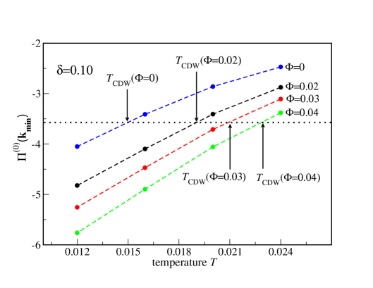
Figure 7: (color online) $\Pi^{(0)}({\bf k}_{{\rm min}})$ as a function of $T$ for several nematic distortions $\Phi$.

The three empty circles in Fig. 6 at the dopings 0.10, 0.09 and 0.08 denote CDW instabilities which lie in the nematic phase. This means that the change of the band structure due to the nematic distortion should be taken into account in calculating these CDW instabilities. Defining the nematic distortion by

$$\Phi=-\sum_{{\bf p},\alpha}\gamma({\bf p})\langle c^{\dagger}_{{\bf p}\alpha}c_{{\bf p}\alpha}\rangle,$$ (18)

we have calculated $\Pi^{(0)}({\bf k})$ for a fixed distortion $\Phi$ as a function of the axial momentum $\bf k$. $\Pi^{(0)}({\bf k})$ shows a well-pronounced minimum near the momentum ${\bf k}_{{\rm min}}$ defined in Fig. 4. The temperature dependence of this minimum is shown in Fig. 7. It crosses the critical line (dotted line) at the temperature $T_{{\rm CDW}}(\Phi)$ which defines the CDW transition temperature for this $\Phi$. The value for $T_{{\rm CDW}}(0)$ can be read off in Fig. 6 and is also shown in Fig. 7. Fig. 7 shows that $T_{{\rm CDW}}(\Phi)$ is a monotonically increasing function of $\Phi$, at least for the considered interval [0,0.04]. This implies that a nematic distortion always increases the CDW transition temperature and thus strengthens the CDW state. This conclusion also agrees with a recent calculations in the three-band model. K. Kawaguchi and Kontani (2017) Fig. 7 implies that the largest transition temperature is obtained for the largest possible value for $\Phi$. Restrictions for the variable $\Phi$ come from the condition that $\Pi^{(0)}({\bf k})$ lies for all momenta k above the critical line. This restricts $\Phi$ approximately to the interval $0.02<\Phi<0.04$ . The monotonic increase of $T_{{\rm CDW}}(\Phi)$ with $\Phi$ leads therefore to the inequality

$$T_{{\rm CDW}}(0.02)<T_{{\rm CDW}}(\Phi)<T_{{\rm CDW}}(0.04)$$

and thus to lower and upper bounds for the observable transtion temperature $T_{{\rm CDW}}$. We have inserted these lower and upper bounds in Fig. 6 for each of the three dopings in form of vertical bars connecting these bounds. The bars lie above the line which connects the open circles which represent $T_{{\rm CDW}}(\Phi=0)$. They are not far away from the empty circles for our considered dopings so that the empty circles may be considered as a reasonable approximation to the CDW instability also in the coexistence region.

Two of the filled squares in Fig. 6 lie in the CDW phase and correspond to instabilities of the CDW state with respect to an infinitesimally small nematic modulation. To describe these instabilities correctly one would have first to obtain the self-consistent CDW order parameter and then to calculate the position where the renormalized $\Pi^{(0)}({\bf k}\sim 0)$ crosses the critical line. Since we have not determined the CDW order parameter the physical relevance of these filled squares remains unclear.

V Conclusions

In conclusion, we have identified in our approach five different charge instabilities in the underdoped region. The leading one corresponds to a nematic transition with a transition temperature $T_{{\rm nem}}$, which decreases strongly and approximately linearly with increasing doping and vanishes near the doping $\delta=0.12$. Below $T_{{\rm nem}}$ there exist secondary charge instabilities with wave vectors ${\bf k}_{1},{\bf k}_{{\rm min}}\approx{\bf k}_{2},{\bf k}_{3}$ and ${\bf k}_{4}$ which are shown in the inset of Fig. 1 and in Figs. 3 and 4. ${\bf k}_{1}$ and ${\bf k}_{4}$ connect nested regions. The associated instabilities are extremely sensitive to temperature and do not play a role for the phase diagram at finite temperatures. The instabilities with wave vectors ${\bf k}_{{\rm min}}$ and ${\bf k}_{3}$ are much more robust and compete with each other. At low doping the minimum in $\Pi^{(0)}({\bf k})$ is much lower near ${\bf k}_{{\rm min}}$ than near ${\bf k}_{3}$. As a result the axial CDW with momentum ${\bf k}_{{\rm min}}$ will be more stable than the flux phase with momentum ${\bf k}_{3}$. With increasing doping the two minima come closer and closer until the absolute minimum has moved to ${\bf k}_{3}$ for $\delta$ larger than 0.12. However, both minima are then in the stable region and neither state represents the ground state. Our calculation leads thus to the result that the axial instability at ${\bf k}_{{\rm min}}$ is always the leading CDW instability and not the flux or any other diagonal instability. This reflects the fact that in our one-band model spin-induced axial charge fluctuations are substantially larger than diagonal ones. Moreover, the leading CDW instability is enhanced if it lies in the nematic phase as shown by the vertical bars in Fig. 6. Interesting is that in the three-band model of Refs. Y. Yamakawa and H. Kontani, 2015; Tsuchiizu et al., 2016 there is no flux phase and the competition between instabilities takes place near the momenta ${\bf k}_{{\rm min}}$ and ${\bf k}_{4}$ and not ${\bf k}_{{\rm min}}$ and ${\bf k}_{3}$. Other differences are that the leading instability is in our case a nematic transition with a wave vector ${\bf k}\sim(0,0)$ and that axial and not diagonal CDWs appear as leading secondary instabilities without further many-body corrections.

VI Acknowledgements

The authors acknowledge useful discussions with M. Bejas, W. Metzner, H. Yamase, M. Minola, and B. Keimer. A.G. thanks the Max-Planck Institut für Festkörperforschung for hospitality.

Appendix A Ladder summation for $\Pi_{rs}(k)$

Let us consider first the ladder contribution to $\Pi_{rs}(k)$ which is linear in $J$. Using the interaction $H^{\prime}$ of Eq. (8) two different diagrams can be drawn for $\Pi_{rs}(k)$ as shown in Fig. 8. Solid lines denote electron Green’s functions, $\gamma_{r}({\bf p})$ and $\gamma_{s}({\bf p})$ are functions defined below Eq. (3). The rectangle originates from the interaction $H^{\prime}$ and is equal to $-J/2\sum_{t}\gamma_{t}({\bf p})\gamma_{t}({\bf p^{\prime}})$ for the upper and equal to $-J/2\sum_{t}\gamma_{t}({\bf p^{\prime}}+{\bf k})\gamma_{t}({\bf p}+{\bf k})$ for the lower diagram. Since $\sum_{t}\gamma_{t}({\bf p})\gamma_{t}({\bf p^{\prime}})$ depends only on the difference ${\bf p}-{\bf p^{\prime}}$ the two factors as well as the two diagrams are equal. This is plausible because interchanging the left and right sides of the rectangle in the upper diagram produces the lower one and vice versa. Adding both diagrams yields $-\sum_{t}\Pi^{(0)}_{rt}(k)J\Pi^{(0)}_{ts}(k)$, i.e., the linear term in $J$ in Eq. (10). $\Pi^{(0)}_{rt}(k)$ is the unperturbed charge Green’s function.

Let us consider now the ladder contributions to $\Pi_{rs}(k)$ of order $J^{n}$. There is one diagram of this order where pairs of electrons connect opposite sides of adjacent rectangles. Interchanging the sides of one or more rectangles produces different diagrams which all have the same value similar as in the case $n=1$ treated above. Summing over all the diagrams, the overall prefactor becomes $(-1)^{n}(J/2)^{n}\times 2^{n}=J^{n}$. Moreover, the electron lines yield a matrix product of $n+1$ matrices $\Pi^{(0)}_{rt}(k)$, i.e., we have obtained the $n$-th order term in $J$ of Eq. (10).

Figure 8: (color online) First-order ladder diagrams for $\Pi_{rs}({k})$. $H^{\prime}$ is the interaction, $\gamma_{r}({\bf p})$ and $\gamma_{s}({\bf p})$ are functions defined below Eq. (3).

Appendix B Evaluation of the AL diagrams

The second diagram in Fig. 1 consists of a product of two identical vertices $V(k,q)$ which are connected by two spin propagators. $V(k,q)$ can be illustrated by a circle consisting of three Green’s functions and a bare vertex $\gamma({\bf p})$. Analytically, $V(k,q)$ is given by

$$V(k;q)=\sum_{p}\gamma({\bf p})G(p)G(p+k)G(p+q).$$ (19)

The sum over $p=({\bf p},{\rm i}\Omega_{n})$ also includes a sum over Matsubara frequencies ${\rm i}\Omega_{n}$ which can be carried out analytically. Writing $q=({\bf q},{\rm i}\nu_{n})$ and considering $z={\rm i}\nu_{n}$ as a general complex variable we get

$$V(k;{\bf q},z)= \sum_{\bf p}\frac{\gamma({\bf p})}{\epsilon_{{\bf p}+{\bf k}}-{\rm i}\omega_{n}-\epsilon_{\bf p}}$$

$$\times\left[\frac{f(\epsilon_{{\bf p}+{\bf k}})-f({\epsilon_{{\bf p}+{\bf q}}})}{z-{\rm i}\omega_{n}+\epsilon_{{\bf p}+{\bf k}}-\epsilon_{{\bf p}+{\bf q}}}\right.$$

$$+\left.\frac{f(\epsilon_{{\bf p}+{\bf q}})-f({\epsilon_{{\bf p}}})}{z+\epsilon_{{\bf p}}-\epsilon_{{\bf p}+{\bf q}}}\right].$$ (20)

Restricting ourselves to the static limit ${\rm i}\omega_{n}=0$ $V({\bf k};{\bf q},z)$ has the spectral representation

$$V({\bf k};{\bf q},z)=\int d\epsilon\frac{{\tilde{B}}({\bf k};{\bf q},\epsilon)}{z-\epsilon},$$ (21)

with the spectral function

$$\tilde{B}({\bf k};{\bf q},\epsilon) =\sum_{\bf p}\frac{\gamma({\bf p})}{\epsilon_{{\bf p}+{\bf k}}-\epsilon_{\bf p}}$$

$$\times\left[(f(\epsilon_{{\bf p}+{\bf k}})-f(\epsilon_{{\bf p}+{\bf q}}))\delta(\epsilon+\epsilon_{{\bf p}+{\bf k}}-\epsilon_{{\bf p}+{\bf q}})\right.$$

$$+\left.(f(\epsilon_{{\bf p}+{\bf q}})-f(\epsilon_{{\bf p}}))\delta(\epsilon+\epsilon_{\bf p}-\epsilon_{{\bf p}+{\bf q}})\right].$$ (22)

The third diagram in Fig. 1 is obtained from the second one by exchanging the right ends of the spin propagators. This does not affect the left vertex but changes the right one to

$${\tilde{V}}(k;q)=\sum_{p}\gamma({\bf p+\bf k})G(p)G(p+k)G(p+q).$$ (23)

Another AL diagram can be generated by exchanging the two ends of the spin propagators in the left vertex. This leaves the right vertex unchanged whereas the left vertex is now given by ${\tilde{V}}(k;q)$. Furthermore, another diagram is obtained by exchanging the two spin propagators yielding a diagram where both vertices are given by ${\tilde{V}}(k;q)$. The first and fourth diagram are topologically equivalent and give identical analytic contributions. The same holds for the second and third diagram. Thus, if the symmetrized vertex $V^{S}$,

$$V^{S}({\bf k};{\bf q},z)=V({\bf k};{\bf q},z)+{\tilde{V}}({-\bf k};{-\bf q},-z),$$ (24)

is used in the second diagram together with a factor 1/2 both topologically inequivalent diagrams are taken into account. From the above also follows that the symmetrized vertex function $V^{S}$ possesses a spectral representation,

$$V^{S}({\bf k};{\bf q},z)=\int d\epsilon\frac{B({\bf k};{\bf q},{\epsilon})}{z-\epsilon},$$ (25)

with a real spectral function $B({\bf k};{\bf q},\epsilon)$. Similarly, the spin propagator $D$ (it is independent of the Cartesian index which allows to drop it), can be written as

$$D({\bf q},{\rm i}\omega_{n})=\int d\epsilon\frac{A({\bf q},\epsilon)}{{\rm i}\omega_{n}-\epsilon}.$$ (26)

with the spectral function $A({\bf q},\epsilon)$. Using the above spectral representations the expression for the AL diagrams becomes

$$\Pi^{(0)}_{AL}({\bf k})= \frac{3}{8}\sum_{\bf q}J^{2}({\bf q})J^{2}({\bf k}-{\bf q})\int d\epsilon d\epsilon^{\prime}dxdx^{\prime}$$

$$A({\bf q},\epsilon)A({\bf k}-{\bf q},\epsilon^{\prime})B(x)B(x^{\prime})S,$$ (27)

$$S=(-1)\oint dz\frac{n(z)}{2\pi{\rm i}}\frac{1}{z-\epsilon}\cdot\frac{1}{z+\epsilon^{\prime}}\cdot\frac{1}{z-x}\cdot\frac{1}{z-x^{\prime}},$$ (28)

$n(z)$ is equal to $1/({\rm exp}(\beta z)-1)$ and $\oint$ a contour integral circling the real axis in the mathematically positive sense. The prefactor (-1) in Eq. (28) arises from changing the sign in the second factor to the right of the sign $\oint$ in Eq. (28). $S$ can also be written as an integral over real $z$,

$$S= (-1)\int_{-\infty}^{\infty}dz\frac{n(z)}{2\pi{\rm i}}\left[\frac{1}{z-{\rm i}\eta-\epsilon}\cdot\frac{1}{z-{\rm i}\eta+\epsilon^{\prime}}\right.$$

$$\cdot\frac{1}{z-{\rm i}\eta-x}\cdot\frac{1}{z-{\rm i}\eta-x^{\prime}}$$

$$-\frac{1}{z+{\rm i}\eta-\epsilon}\cdot\frac{1}{z+{\rm i}\eta+\epsilon^{\prime}}$$

$$\left.\cdot\frac{1}{z+{\rm i}\eta-x}\cdot\frac{1}{z+{\rm i}\eta-x^{\prime}}\right],$$ (29)

where $\eta$ is a positive infinitesimal.

A straightforward evaluation of the contour integral in Eq. (29) in terms of additive pole contributions along the real axis encounters some difficulties. For instance, if we take the pole contribution from the first factor in Eq. (28) we have to insert $z=\epsilon$ in the remaining factors under the integral. The third factor would lead to $V^{S}({\bf k};{\bf q},\epsilon)$, i.e., a Green’s function where the frequency lies exactly on the cut. Clearly, such a divergence will be canceled by a zero in the numerator. Such a compensation is, however, difficult to achieve, both numerically and analytically. We therefore present below a way where Green’s functions never have to be taken exactly on the real axis and the compensation of singularities is done automatically. Let us introduce the functions

$$g_{1}^{\pm}=\frac{1}{z\mp{\rm i}\eta-\epsilon},$$ (30)

$$g_{2}^{\pm}=\frac{1}{z\mp{\rm i}\eta+\epsilon^{\prime}},$$ (31)

$$g_{3}^{\pm}=\frac{1}{z\mp{\rm i}\eta-x},$$ (32)

$$g_{4}^{\pm}=\frac{1}{z\mp{\rm i}\eta-x^{\prime}},$$ (33)

and also

$$h_{i}^{\pm}=(g_{i}^{+}\pm g_{i}^{-})/2,\;\;\;\;i=1,..,4.$$ (34)

It follows that

$$g_{i}^{+}=h_{i}^{+}+h_{i}^{-},\;\;\;g_{i}^{-}=h_{i}^{+}-h_{i}^{-},\;\;\;\;i=1,..,4,$$ (35)

and thus

$$h_{i}^{+}={\rm Re}g_{i}^{+},\;\;\;h_{i}^{-}={\rm i}{\rm Im}g_{i}^{+},\;\;\;\;i=1,...4.$$ (36)

The content of the large parantheses in Eq. (29) can be written as,

$$\{\}=\Pi_{i=1}^{4}g_{i}^{+}-\Pi_{i=1}^{4}g_{i}^{-}=$$ (37)

$$\Pi_{i=1}^{4}(h_{i}^{+}+h_{i}^{-})-\Pi_{i=1}^{4}(h_{i}^{+}-h_{i}^{-})=$$ (38)

$$2(h_{1}^{-}h_{2}^{+}+h_{1}^{+}h_{2}^{-})(h_{3}^{+}h_{4}^{+}+h_{3}^{-}h_{4}^{-})$$

$$+2(h_{3}^{+}h_{4}^{-}+h_{3}^{-}h_{4}^{+})(h_{1}^{+}h_{2}^{+}+h_{1}^{-}h_{2}^{-}).$$ (39)

{ } contains only odd powers of the imaginary unit ${\rm i}$. Taking also the prefactor $1/(2\pi{\rm i})$ into account it follows that $\Pi^{(0)}_{AL}({\bf k})$ is real, as it should be. The first term in Eq. (39) represents pole contributions from spin propagators, the second one from vertices.

To evaluate the expression in Eq. (39) we split it into several contributions:

$$(A) \;\;\;\;\;2h_{1}^{-}h_{2}^{+}(h_{3}^{+}h_{4}^{+}+h_{3}^{-}h_{4}^{-})=$$

$$2{\rm i}{\rm Im}g_{1}^{+}\cdot{\rm Re}g_{2}^{+}({\rm Re}g_{3}^{+}\cdot{\rm Re}g_{4}^{+}-{\rm Im}g_{3}^{+}\cdot{\rm Im}g_{4}^{+}).$$ (40)

Taking the complete expression into account we find the following contribution to $\Pi^{(0)}_{AL}({\bf k})$:

$$\frac{3}{8}\sum_{\bf q} J^{2}({\bf q})J^{2}({\bf k}-{\bf q})\int d\epsilon\;n(\epsilon)A({\bf q},\epsilon){\rm Re}D({\bf k}-{\bf q},-\epsilon)$$

$$\times\left[({\rm Re}V^{S}({\bf k},{\bf q},\epsilon))^{2}-({\rm Im}V^{S}({\bf k},{\bf q},\epsilon))^{2}\right],$$ (41)

where retarded boundary conditions are applied to the Green’s functions $D$ and $V^{S}$.

$$(B) \;\;\;\;\;2h_{1}^{+}h_{2}^{-}(h_{3}^{+}h_{4}^{+}+h_{3}^{-}h_{4}^{-})=$$

$$2{\rm Re}g_{1}^{+}\cdot{\rm i}{\rm Im}g_{2}^{+}({\rm Re}g_{3}^{+}\cdot{\rm Re}g_{4}^{+}-{\rm Im}g_{3}^{+}\cdot{\rm Im}g_{4}^{+}).$$ (42)

The resulting contribution to $\Pi^{(0)}_{AL}({\bf k})$ is,

$$\frac{3}{8}\sum_{\bf q} J^{2}({\bf q})J^{2}({\bf k}-{\bf q})\int d\epsilon\;n(\epsilon){\rm Re}D({\bf q},\epsilon)A({\bf k}-{\bf q},\epsilon)$$

$$\times\left[({\rm Re}V^{S}({\bf k},{\bf q},\epsilon))^{2}-({\rm Im}V^{S}({\bf k},{\bf q},\epsilon))^{2}\right].$$ (43)

$$(C) \;\;\;\;\;2h_{3}^{+}h_{4}^{-}(h_{1}^{+}h_{2}^{+}+h_{1}^{-}h_{2}^{-})=$$

$$2{\rm Re}g_{3}^{+}\cdot{\rm i}{\rm Im}g_{4}^{+}({\rm Re}g_{1}^{+}\cdot{\rm Re}g_{2}^{+}-{\rm Im}g_{1}^{+}\cdot{\rm Im}g_{2}^{+}).$$ (44)

The resulting contribution to $\Pi^{(0)}_{AL}({\bf k})$ is,

$$\frac{3}{8}\sum_{\bf q} J^{2}({\bf q})J^{2}({\bf k}-{\bf q})\int d\epsilon\;n(\epsilon)B(\epsilon){\rm Re}V^{S}({\bf k},{\bf q},\epsilon)$$

$$\times \left[{\rm Re}D({\bf q},\epsilon){\rm Re}D({\bf k}-{\bf q},\epsilon)\right.$$

$$\left.-{\rm Im}D({\bf q},\epsilon){\rm Im}D({\bf k}-{\bf q},\epsilon)\right].$$ (45)

$$(D)\;\;\;\;\;2h_{3}^{-}h_{4}^{+}(h_{1}^{+}h_{2}^{+}+h_{1}^{-}h_{2}^{-}).$$ (46)

This contribution is identical with that of case (C). Adding all contributions yields

$$\Pi_{AL}^{(0)}({\bf k}) =\frac{3}{8}\sum_{\bf q}J^{2}({\bf q})J^{2}({\bf k}-{\bf q})\int d\epsilon\;n(\epsilon)\Big{\{}$$

$$\left[A({\bf q},\epsilon){\rm Re}D({\bf k}-{\bf q},-\epsilon)+{\rm Re}D({\bf q},\epsilon)A({\bf k}-{\bf q},\epsilon)\right]$$

$$\times\left[({\rm Re}V^{S}({\bf k},{\bf q},\epsilon))^{2}-({\rm Im}V^{S}({\bf k},{\bf q},\epsilon))^{2}\right]$$

$$+2B(\epsilon){\rm Re}V^{S}({\bf k},{\bf q},\epsilon)$$

$$\times\left[{\rm Re}D({\bf q},\epsilon){\rm Re}D({\bf k}-{\bf q},\epsilon)\right.$$

$$-\left.{\rm Im}D({\bf q},\epsilon){\rm Im}D({\bf k}-{\bf q},\epsilon)\right]\Big{\}}$$ (47)

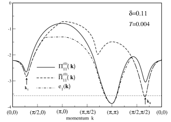
Figure 9: (color online) Lowest-order (bubble) contribution to $\Pi^{(0)}_{11}({\bf k})$, $\bar{\Pi}^{(0)}_{11}({\bf k})$ and to the lowest eigenvalue $e_{1}({\bf k})$ of $\Pi^{(0)}_{rs}({\bf k})$.

Appendix C Charge fluctuations with general symmetries

Keeping all 4 symmetry channels the static susceptibility becomes a 4x4 matrix $\Pi_{rs}({\bf k})$ which satisfies Eq. (10), i.e.,

$$\Pi_{rs}({\bf k})=\sum_{t}\Pi^{(0)}_{rt}(1+J\Pi^{(0)}({\bf k}))^{-1}_{ts}.$$ (48)

The matrix $\Pi^{(0)}_{rs}$ can be diagonalized by a unitary transformation $U$,

$$\Pi^{(0){\prime}}_{tt}({\bf k})=\sum_{rs}U_{tr}\Pi^{(0)}_{rs}({\bf k})U^{\dagger}_{st}.$$ (49)

Eq. (48) becomes then

$$\Pi^{\prime}_{tt}({\bf k})=\frac{\Pi^{(0){\prime}}_{tt}({\bf k})}{1+J{\Pi^{(0){\prime}}_{tt}({\bf k})}}.$$ (50)

A charge instability with symmetry $v$, wave vector ${\bf k}_{c}$ and transition temperature $T_{\rm c}$ requires that $\Pi^{(0){\prime}}_{tt}({\bf k})$ has a minimum and a positive curvature at ${\bf k}_{c}$. Furthermore, the temperature $T_{\rm c}$ must be such that $\Pi^{(0){\prime}}_{tt}({\bf k}_{c})=-1/J$. Alternatively, one can say that at the transition temperature ${T_{\rm c}}$ $\Pi^{(0){\prime}}_{tt}({\bf k})$ touches as a function of ${\bf k}$ the critical line $-1/J$ at ${\bf k}_{\rm c}$ from above.

In section IV we limited ourselves to the basis function $r=1$ and considered $\Pi^{(0)}_{11}({\bf k})$ and not $\Pi^{{(0)}\prime}_{11}({\bf k})$, which is the lowest eigenvalue $e_{1}({\bf k})$ of the matrix $\Pi^{(0)}_{rs}({\bf k})$. Keeping only $r=1$ is a good approximation if $\Pi^{(0)}_{11}({\bf k})$ and $\Pi^{{(0)}\prime}_{11}({\bf k})$ are close to each other near the instabilities. The first instability $M1$ has the wave vector ${\bf k}_{{\rm nem}}=(k_{{\rm nem}},0)$ and the transition temperature $T_{{\rm nem}}$ which implies $\Pi^{(0)}_{11}({\bf k}_{{\rm nem}})=-1/J\approx-3.571$. For doping $\delta=0.08$ we obtain $e_{1}({\bf k}_{{\rm nem}})=-3.522$, for $\delta=0.11$ $e_{1}({\bf k}_{{\rm nem}})=-3.551$. The approximation to keep only $r=1$ is thus extremely well fulfilled. The second instability $M2$ has the wave vector ${\bf k}_{{\rm min}}=(k_{{\rm min}},0)$ and the transition temperature $T_{{\rm CDW}}$ which again implies $\Pi^{(0)}_{11}({\bf k}_{{\rm min}})=-1/J\approx-3.571$. For doping $\delta=0.08$ we obtain $e_{1}({\bf k}_{{\rm min}})=-4.097$, for $\delta=0.11$ $e_{1}({\bf k}_{{\rm min}})=-4.025$. The interaction between different density variables is at $M2$ substantially larger than at $M1$. Nevertheless, the $d$-wave component dominates also at $M2$, as can be seen from the eigenvector belonging to $e_{1}({\bf k}_{{\rm min}})$: For $\delta=0.08$ we have $U_{11}=0.903,U_{21}=-0.265,U_{31}=U_{41}=-0.239$, for $\delta=0.11$ $U_{11}=0.922,U_{21}=-0.161,U_{31}=U_{41}=-0.249$. Thus the critical density fluctuation $\sum_{r}U_{r1}n_{r}({\bf k})$ is always dominated by its d-wave part.

Some authors prefer to define charge variables by

$${\bar{n}}_{r}({\bf k})=\sum_{{\bf p},\alpha}\gamma_{r}({\bf p})c^{\dagger}_{{\bf p}+{\bf k}/2,\alpha}c_{{\bf p}-{\bf k}/2,\alpha},$$ (51)

and Green’s functions ${\bar{\Pi}}^{(0)}_{rs}({\bf k})$ by Eq. (9) with $n_{r}({\bf k},\tau_{1})$ and $n^{\dagger}_{s}({\bf k},\tau_{2})$ replaced by ${\bar{n}}_{r}({\bf k},\tau_{1})$ and ${\bar{n}}^{\dagger}_{s}({\bf k},\tau_{2})$, respectively. Shifting $\bf p$ to ${\bf p}+{\bf k}/2$ in the sum over ${\bf p}$ and decomposing the trigonometric functions in $\gamma_{r}$ one recognizes that the two sets of density variables are related to each other by a unitary transformation. This means that the corresponding static Green’s functions $\Pi^{(0)}_{rs}({\bf k})$ and $\bar{\Pi}^{(0)}_{rs}({\bf k})$ are also related by a unitary transformation and have the same eigenvalues. The condition for charge instabilities is thus independent of the choice of density variables. This, however, is in general not true if one truncates the matrices to scalars. For instance, if one approximates $\Pi^{(0)}_{rs}({\bf k})$ and ${\bar{\Pi}}^{(0)}_{rs}({\bf k})$ by the bubble contribution, $\Pi^{(0)}_{11}({\bf k})$ and $\bar{\Pi}^{(0)}_{11}({\bf k})$ are given by the solid and dashed lines in Fig. 9, respectively. In the same approximation the dash-dotted line in that figure depicts the lowest eigenvalue $e_{1}({\bf k})$ of the matrix $\Pi^{(0)}_{rs}({\bf k})$. The three curves are close to each other at small momenta ${\bf k}$, that is, near ${\bf k}_{1}$ and ${\bf k}_{4}$, as one may expect from the definition of the density variables. However, for momenta ${\bf k}$ near $(\pi,\pi)$ only the solid line is close to the dash-dotted line whereas the dashed line lies much higher and well above the critical value $-1/J\approx-3.571$. This means that the flux instability is lost if $r=1$ and Eq. (51) are used. In this case the choice Eq. (4) is certainly preferable to that of Eq. (51).

References

- M. Vojta (2009) M. Vojta, Adv. Phys. 58, 699 (2009).
- Fradkin et al. (2010) E. Fradkin, S. Kivelson, M. Lawler, J. Eisenstein, and A. Mackenzie, Annual Review of Condensed Matter Physics 1, 153 (2010).
- Kivelson et al. (1998) S. A. Kivelson, E. Fradkin, and V. J. Emery, Nature (London) 393, 550 (1998).
- Kivelson et al. (2003) S. A. Kivelson, I. P. Bindloss, E. Fradkin, V. Oganesyan, J. M. Tranquada, A. Kapitulnik, and C. Howald, Rev. Mod. Phys. 75, 1201 (2003).
- Wu et al. (2011) T. Wu, H. Mayaffre, S. Krämer, M. Horvatić, C. Berthier, W. N. Hardy, R. Liang, D. A. Bon, and M.-H. Julien, Nature 477, 191 (2011).
- Ghiringhelli et al. (2012) G. Ghiringhelli, M. LeTacon, M. Minola, S. Blanco-Canosa, C. Mazzoli, N. B. Brookes, G. M. D. Luca, A. Frano, D. G. Hawthorn, F. He, T. Loew, M. M. Sala, D. C. Peets, M. Salluzzo, E. Schierle, R. Sutarto, G. A. Sawatzky, E. Weschke, B. Keimer, and L. Braicovich, Science 337, 821 (2012).
- Chang et al. (2012) J. Chang, E. Blackburn, A. T. Holmes, N. B. Christensen, J. Larsen, J. Mesot, R. Liang, D. A. Bonn, W. N. Hardy, A. Watenphul, M. v. Zimmermann, E. M. Forgan, and S. M. Hayden, Nat. Phys. 8, 871 (2012).
- Achkar et al. (2012) A. J. Achkar, R. Sutarto, X. Mao, F. He, A. Frano, S. Blanco-Canosa, M. LeTacon, G. Ghiringhelli, L. Braicovich, M. Minola, M. Moretti Sala, C. Mazzoli, R. Liang, D. A. Bonn, W. N. Hardy, B. Keimer, G. A. Sawatzky, and D. G. Hawthorn, Phys. Rev. Lett. 109, 167001 (2012).
- Blackburn et al. (2013) E. Blackburn, J. Chang, M. Hücker, A. T. Holmes, N. B. Christensen, R. Liang, D. A. Bonn, W. N. Hardy, U. Rütt, O. Gutowski, M. v. Zimmermann, E. M. Forgan, and S. M. Hayden, Phys. Rev. Lett. 110, 137004 (2013).
- LeBoeuf et al. (2013) D. LeBoeuf, S. Krämer, W. N. Hardy, R. Liang, D. A. Bonn, and C. Proust, Nat. Phys. 9, 79 (2013).
- Blanco-Canosa et al. (2014) S. Blanco-Canosa, A. Frano, E. Schierle, J. Porras, T. Loew, M. Minola, M. Bluschke, E. Weschke, B. Keimer, and M. LeTacon, Phys. Rev. B 90, 054513 (2014).
- Comin et al. (2014) R. Comin, A. Frano, M. M. Yee, Y. Yoshida, H. Eisaki, E. Schierle, E. Weschke, R. Sutarto, F. He, A. Soumyanarayanan, Y. He, M. LeTacon, I. S. Elfimov, J. E. Hoffman, G. A. Sawatzky, B. Keimer, and A. Damascelli, Science 343, 390 (2014).
- da Silva Neto et al. (2014) E. H. da Silva Neto, P. Aynajian, A. Frano, R. Comin, E. Schierle, E. Weschke, A. Gyenis, J. Wen, J. Schneeloch, Z. Xu, S. Ono, G. Gu, M. LeTacon, and A. Yazdani, Science 343, 393 (2014).
- Hashimoto et al. (2014) M. Hashimoto, G. Ghiringhelli, W.-S. Lee, G. Dellea, A. Amorese, C. Mazzoli, K. Kummer, N. B. Brookes, B. Moritz, Y. Yoshida, H. Eisaki, Z. Hussain, T. P. Devereaux, Z.-X. Shen, and L. Braicovich, Phys. Rev. B 89, 220511 (2014).
- Tabis et al. (2014) W. Tabis, Y. Li, M. LeTacon, L. Braicovich, A. Kreyssig, M. Minola, G. Dellea, E. Weschke, M. J. Veit, M. Ramazanoglu, A. I. Goldman, T. Schmitt, G. Ghiringhelli, N. Barišić, M. K. Chan, C. J. Dorow, G. Yu, X. Zhao, B. Keimer, and M. Greven, Nat. Commun. 5, 5875 (2014).
- Gerber et al. (2015) S. Gerber, H. Jang, H. Nojiri, S. Matsuzawa, H. Yasumura, D. A. Bonn, R. Liang, W. N. Hardy, Z. Islam, A. Mehta, S. Song, M. Sikorski, D. Stefanescu, Y. Feng, S. A. Kivelson, T. P. Devereaux, Z. X. Shen, C. C. Kao, W. S. Lee, D. Zhu, , and J. S. Lee, Science 350, 949 (2015).
- Y. Y. Peng, M. Salluzzo, X. Sun, A. Ponti, D. Betto, A. M. Ferretti, F. Fumagalli, K. Kummer, M. LeTacon, X. J. Zhou, N. B. Brookes, L. Braicovich, and G. Ghiringhelli (2016) Y. Y. Peng, M. Salluzzo, X. Sun, A. Ponti, D. Betto, A. M. Ferretti, F. Fumagalli, K. Kummer, M. LeTacon, X. J. Zhou, N. B. Brookes, L. Braicovich, and G. Ghiringhelli, Phys. Rev. B 94, 184511 (2016).
- Tabis et al. (2017) W. Tabis, B. Yu, I. Bialo, M. Bluschke, T. Kolodziej, A. Kozlowski, Y. Tang, E. Weschke, B. Vignolle, M. Hepting, H. Gretarsson, R. Sutarto, F. He, M. LeTacon, N. Barisik, G. Yu, and M. Greve, Phys. Rev. B 96, 134510 (2017).
- K. Yamada, C. H. Lee, K. Kurahashi, J. Wada, S. Wakimoto, S. Ueki, H. Kimura, Y. Endoh, S. Hosoya, G. Shirane, R. J. Birgeneau, M. Greven, M. A. Kastner, and Y. J. Kim (1998) K. Yamada, C. H. Lee, K. Kurahashi, J. Wada, S. Wakimoto, S. Ueki, H. Kimura, Y. Endoh, S. Hosoya, G. Shirane, R. J. Birgeneau, M. Greven, M. A. Kastner, and Y. J. Kim, Phys. Rev. B 57, 6165 (1998).
- Haug et al. (2010) D. Haug, V. Hinkov, Y. Sidis, P. Bourges, N. B. Christensen, A. Ivanov, T. Keller, C. T. Lin, and B. Keimer, New J. Phys. 12, 105006 (2010).
- M. Hücker, M. v. Zimmermann, G. D. Gu, Z. J. Xu, J. S. Wen, G. Xu, H. J. Kang, A. Zheludev, and J. M. Tranquada (2011) M. Hücker, M. v. Zimmermann, G. D. Gu, Z. J. Xu, J. S. Wen, G. Xu, H. J. Kang, A. Zheludev, and J. M. Tranquada, Phys. Rev. B 83, 104506 (2011).
- M. H. Hamidian, S. D. Edkins, Chung Koo Kim, J. C. Davis, A. P. Mackenzie, H. Eisaki, S. Uchida, M. J. Lawler, E.-A. Kim, S. Sachdev, and K. Fujita (2016) M. H. Hamidian, S. D. Edkins, Chung Koo Kim, J. C. Davis, A. P. Mackenzie, H. Eisaki, S. Uchida, M. J. Lawler, E.-A. Kim, S. Sachdev, and K. Fujita, Nat. Phys. 12, 150 (2016).
- Cyr-Choinière et al. (2018) O. Cyr-Choinière, R. Daou, F. Laliberté, C. Collignon, S. Badoux, D. LeBoeuf, J. Chang, B. J. Ramshaw, D. A. Bonn, W. N. Hardy, R. Liang, J.-Q. Yan, J.-G. Cheng, J.-S. Zhou, J. B. Goodenough, S. Pyon, T. Takayama, H. Takagi, N. Doiron-Leyraud, and L. Taillefer, Phys. Rev. B 97, 064502 (2018).
- Atkinson et al. (2015) W. Atkinson, A. Kampf, and S. Bulut, New J. Phys. 17, 013025 (2015).
- Atkinson et al. (2016) W. A. Atkinson, A. P. Kampf, and S. Bulut, Phys. Rev. B 93, 134517 (2016).
- Yamase and Kohno (2000a) H. Yamase and H. Kohno, J. Phys. Soc. Jpn. 69, 332 (2000a).
- Yamase and Kohno (2000b) H. Yamase and H. Kohno, J. Phys. Soc. Jpn. 69, 2151 (2000b).
- Cappelluti and Zeyher (1999) E. Cappelluti and R. Zeyher, Phys. Rev. B 59, 6475 (1999).
- Halboth and Metzner (2000) C. J. Halboth and W. Metzner, Phys. Rev. Lett. 85, 5162 (2000).
- Yamase and Metzner (2007) H. Yamase and W. Metzner, Phys. Rev. B 75, 155117 (2007).
- M. A. Metlitski and S. Sachdev (2010) M. A. Metlitski and S. Sachdev, New J. Phys. 12, 105007 (2010).
- Husemann and Metzner (2012) C. Husemann and W. Metzner, Phys. Rev. B 86, 085113 (2012).
- Bejas et al. (2012) M. Bejas, A. Greco, and H. Yamase, Phys. Rev. B 86, 224509 (2012).
- Sachdev and LaPlaca (2013) S. Sachdev and R. LaPlaca, Phys. Rev. Lett. 111, 027202 (2013).
- Allais et al. (2014) A. Allais, J. Bauer, and S. Sachdev, Phys. Rev. B 90, 155114 (2014).
- Sau and Sachdev (2014) J. D. Sau and S. Sachdev, Phys. Rev. B 89, 075129 (2014).
- Efetov et al. (2013) K. B. Efetov, H. Meier, and C. Pépin, Nat. Phys. 9, 442 (2013).
- Wang and Chubukov (2014) Y. Wang and A. Chubukov, Phys. Rev. B 90, 035149 (2014).
- Mishra and Norman (2015) V. Mishra and M. R. Norman, Phys. Rev. B 92, 060507 (2015).
- P. A. Volkov and K. B. Efetov (2016) P. A. Volkov and K. B. Efetov, J. Supercond. Novel Magn. 29, 1069 (2016).
- Y. Yamakawa and H. Kontani (2015) Y. Yamakawa and H. Kontani, Phys. Rev. Lett. 114, 257001 (2015).
- Tsuchiizu et al. (2016) M. Tsuchiizu, Y. Yamakawa, and H. Kontani, Phys. Rev. B 93, 155148 (2016).
- F.C. Zhang and T.M. Rice (1988) F.C. Zhang and T.M. Rice, Phys. Rev. B 37, 3759 (1988).
- Aslamasov and Larkin (1968) L. Aslamasov and A. Larkin, Phys. Lett. A 26, 238 (1968).
- Caprara et al. (2015) S. Caprara, M. Colonna, C. Di Castro, R. Hackl, B. Mutschler, L. Tassini, and M. Grilli, Phys. Rev. B 91, 205115 (2015).
- Kampf and Brenig (1992) A. Kampf and W. Brenig, Z. Physik B 89, 313 (1992).
- Liu et al. (2016) Y.-H. Liu, R. M. Konik, T. M. Rice, and F.-C. Zhang, Nature Commun. 7, 10378 (2016).
- Chowdhury and Sachdev (2014) D. Chowdhury and S. Sachdev, Phys. Rev. B 90, 134516 (2014).
- Zeyher and Kulić (1996) R. Zeyher and M. L. Kulić, Phys. Rev. B 54, 8985 (1996).
- Greco and Zeyher (2006) A. Greco and R. Zeyher, Phys. Rev. B 73, 195126 (2006).
- Brinckmann and Lee (1999) J. Brinckmann and P. A. Lee, Phys. Rev. Lett. 82, 2915 (1999).
- Norman (2001) M. R. Norman, Phys. Rev. B 63, 092509 (2001).
- T. Holder and W. Metzner (2012) T. Holder and W. Metzner, Phys. Rev. B 85, 165130 (2012).
- Sherman (2004) A. Sherman, Phys. Rev. B 70, 184512 (2004).
- A.A. Vladimirov, D. Ihle, and N.M. Plakida (2009) A.A. Vladimirov, D. Ihle, and N.M. Plakida, Phys. Rev. B 80, 104425 (2009).
- Tacon et al. (2011) M. L. Tacon, G. Ghiringhelli, J. Chaloupka, M. M. Sala, V. Hinkovand, M. W. Haverkort, M. Minola, M. Bakr, K. J. Zhou, S. Blanco-Canosa, C. Monney, Y. T. Song, G. L. Sun, C. T. Lin, G. M. D. Luca, M. Salluzzo, G. Khaliullin, T. Schmitt, L. Braicovich, and B. Keimer, Nat. Phys. 7, 725 (2011).
- R. Pietig, R. Bulla, and S. Blawid (1999) R. Pietig, R. Bulla, and S. Blawid, Phys. Rev. Lett. 82, 4046 (1999).
- Y. Sato, S. Kasahara, H. Murayama, Y. Kasahara, E.-G. Moon, T. Nishizaki, T. Loew, J.Porra, B. Keimer, T. Shibauchi and Y. Matsuda (2017) Y. Sato, S. Kasahara, H. Murayama, Y. Kasahara, E.-G. Moon, T. Nishizaki, T. Loew, J.Porra, B. Keimer, T. Shibauchi and Y. Matsuda, Nature Physics 13, 1074 (2017).
- K. Kawaguchi and Kontani (2017) M. T. K. Kawaguchi, Y. Yamakawa and H. Kontani, J. Phys. Soc. Jpn. 86, 063707 (2017).