Stability of a modified Jordan-Brans-Dicke theory in the dilatonic frame

Abstract

We investigate the Jordan-Brans-Dicke action in the cosmological scenario of FLRW spacetime with zero spatially curvature and with an extra scalar field minimally coupled to gravity as matter source. The field equations are studied in two ways. The method of group invariant transformations, i.e., symmetries of differential equations apply in order to constraint the free functions of the theory and determine conservation laws for the gravitational field equations. The second method that we apply for the study of the evolution of the field equations is the stability analysis of equilibrium points. Particularly, we find solutions with $w_{\text{tot}}=-1$, and we study their stability by means of the Center Manifold Theorem. We show this solution is an attractor in the dilatonic frame but it is an intermediate accelerated solution $a\simeq e^{At^{p}},p:=\frac{2}{2+l},\quad\frac{32}{57+6\omega_{0}}<p<\frac{2}{3},\;\text{as}\;t\rightarrow\infty$, and not de Sitter solution. The exponent $p$ is reduced, in a particular case, to the exponent already found for the Jordan’s and Einstein’s frames by A. Cid, G. Leon and Y. Leyva, JCAP 1602, no. 02, 027 (2016). We obtain some equilibrium points which represent stiff solutions. Additionally, we find solutions that can be a phantom solution, a solution with $w_{\text{tot}}=-1$ or a quintessence solution. Other equilibrium points mimic a standard dark matter source ($0<w_{\text{tot}}<1$), radiation ($w_{\text{tot}}=\frac{1}{3}$), among other interesting features. For the dynamical system analysis we develop an extension of the method of $F$-devisers. The new approach relies upon two arbitrary functions $h(\lambda,s)$ and $F(s)$. The main advantage of this procedure allows us to perform a phase-space analysis of the cosmological model without the need for specifying the potentials, revealing the full capabilities of the model.

1 Introduction

Various models have been proposed for the explanation of the results which is followed from the detailed analysis of the recent cosmological data Teg ; Kowal ; Komatsu ; suzuki11 ; Ade15 . The observable late time acceleration have been attributed to the so-called cosmological fluid Dark energy. The nature of dark energy is unknown and the theoretical approaches to the problem can be classified in two categories. The first category: the context of General Relativity an “exotic” matter source which is introduced and provides the late time acceleration of the universe Ar1 ; Ar2 ; Ar3 ; Ar4 ; Ar5 . On the other hand, the second category: the expansion of the universe is attributed to terms which follow from the modification of General Relativity (GR), see for instance ref1 ; ref2 ; ref3 ; ref4 ; ref5 ; ref6 ; ref7 and references therein. In the latter theories the new terms, which follow from the modification of the Einstein-Hilbert action, provide a geometric explanation for the acceleration of the universe.

Scalar fields have played an important role on the Dark energy problem during the last decades. The main characteristic of scalar fields is that they provide new dynamical variables in the gravitational field equations, which can modify the evolution of the field equations to describe the observations. In addition, scalar fields provide the main mechanism to explain the early accelerated era of the universe known as inflation guth . Quintessence is one of the most simplest scalar field model Ar1 which has many interesting applications in the literature qqq01 ; qqq02 ; qqq03 . Phantom scalar field is an extension of the quintessence model, where the scalar field has a non-canonical negative kinetic energy term. The main characteristic of the phantom field is that the equation of state parameter for the cosmological fluid is below the boundary of the cosmological constant ($w=-1$). However, there exist ghosts in that specific model lurena . Quintom scalar field models consist in two scalar fields: a quintessence field and a phantom field. The main property of the quintom models is that in general, the two scalar fields are minimally coupled and they can interact in the kinetic part (and in some models are proposed interactions through the potential function). In the quintom model, the dark energy equation of state parameter can cross the phantom divide line without the presence of ghosts quin00 ; Guo:2004fq ; Feng:2004ff ; Wei:2005nw ; Zhang:2005eg ; Zhang:2005kj ; Lazkoz:2006pa ; Lazkoz:2007mx ; Setare:2008pz ; Setare:2008pc ; Leon:2008aq ; Leon:2012vt ; Leon:2014bta ; Leon:2018lnd ; Mishra:2018dzq ; Marciu:2019cpb ; Marciu:2020vve ; Dimakis:2020tzc .

Another two scalar field cosmological model, which has played a significant role in the description of the early-time acceleration phase of the universe, is the Chiral cosmology. The theory is defined in the Einstein frame where the two kinetic energy of the scalar fields defines a two-dimensional manifold of constant nonzero curvature atr6 ; atr7 . While, the equation of state parameter of the dark energy fluid in Chiral cosmology is bounded by the values one and minus one. In a recent study ndch it was found that under a quantum transition during the early universe the equation of state parameter can cross the phantom divide line and be unbounded and vice versa. In particular, it can be seen as a model to describe all the components of the dark sector of the universe, i.e. the dark energy and the dark matter anchiral1 . It is clear that multi-scalar field models can provide a simple mechanism, generated by the variation of an Action Integral, such that to describe various epochs of the cosmological history Paliathanasis:2018vru ; Elizalde:2004mq ; Elizalde:2008yf .

In the context of this work, we are interested on the Brans-Dicke gravitational action in cosmological studies: the so-called Brans-Dicke theory (BDT). Brans and Dicke in 1961 proposed a gravitational action which satisfies Mach’s principle bdpaper , as the prototype of Scalar-tensor theories (STT). In general, Scalar-tensor theories (STT) of gravity bdpaper ; Wagoner:1970vr ; OHanlon:1972sdp ; OHanlon:1972ysn ; Bekenstein:1977rb ; Bergmann:1968ve ; Nordtvedt:1970uv are supported by fundamental physical theories like superstring theory Green:1996bh . The scalar field of BDT says that $\Phi,$ acts as the source for the gravitational coupling with a varying Newtonian “constant” $G\sim\Phi^{-1}.$ This theory satisfies several observational tests including Solar System tests Abramovici:1992ah and Big-Bang nucleosynthesis constraints Serna:2002fj ; Serna:1995tr . In extension, the BD parameter $\omega(\Phi),$ can vary depending on the scalar field. Additionally, a non-zero self-interaction potential $V(\Phi),$ can be incorporated. Also, the resulting theory survives astrophysical tests Will:1993ns ; Will:2005va ; Barrow:1996kc . On the other hand, some “Extended” inflationary models can be found in Barrow:1990nv ; Faraoni:2006ik ; Liddle:1991am ; La:1989za where the BDT is used as the correct theory of gravity. In this case, the vacuum energy leads directly to a powerlaw solution Mathiazhagan:1984vi , while the exponential expansion can be obtained when a cosmological constant is inserted explicitly into the field equations Barrow:1990nv ; Kolitch:1994kr ; Romero:1992ci .

The action for a general class of STT, can be written in the so-called Einstein frame (EF) as Kaloper:1997sh :

$$S_{EF}=\int_{M_{4}}d{}^{4}x\sqrt{|g|}\left\{\frac{1}{2}R-\frac{1}{2}(\nabla\phi)^{2}-V(\phi)+\Phi(\phi)^{-2}\mathcal{L}_{matter}(\mu,\nabla\mu,\Phi(\phi)^{-1}g_{\alpha\beta})\right\},$$ (1)

where $R$ is the curvature scalar, $\phi$ is the scalar field, related via conformal transformations with the (Brans-Dicke) field $\Phi$, $(\nabla\phi)^{2}$ denotes $g^{\mu\nu}\nabla_{\mu}\phi\nabla_{\nu}\phi$, where denotes $\nabla_{\alpha}$ is the covariant derivative; $V(\phi)$ is the quintessence self-interaction potential, $\Phi(\phi)^{-2}$ is the coupling function, $\mathcal{L}_{matter}$ is the matter Lagrangian, $\mu$ is a collective name for the matter degrees of freedom. The energy-momentum matter tensor is defined by

$$T_{\alpha\beta}=-\frac{2}{\sqrt{|g|}}\frac{\delta}{\delta g^{\alpha\beta}}\left\{\sqrt{|g|}\Phi^{-2}\mathcal{L}(\mu,\nabla\mu,\Phi^{-1}g_{\alpha\beta})\right\}.$$ (2)

The issue of regularity of conformal transformations, or the equivalence of Einstein and Jordan frames have been studied in detail in Magnano:1990qu ; Cotsakis:1993vm ; Teyssandier:1995wr ; Schmidt:1995ws ; Cotsakis:1995wt ; Capozziello:1996xg ; Magnano:1993bd ; Faraoni:1998qx ; Faraoni:2007yn ; Faraoni:2006fx and references therein. Using the conformal transformation $\bar{g}_{\alpha\beta}=\Phi(\phi)^{-1}$ “constant” $\omega(\Phi)$ in such way that
$d\phi=\pm\sqrt{\omega(\Phi)+3/2}\Phi^{-1}d\Phi$ and redefining $\bar{V}(\Phi)=\Phi^{2}V(\phi(\Phi))$ the action (1) can be written in the Jordan frame (JF) as (see Coley:2003mj ):

$$S_{JF}=\int_{M_{4}}d{}^{4}x\sqrt{|\bar{g}|}\left\{\frac{1}{2}\Phi\bar{R}-\frac{1}{2}\frac{\omega(\Phi)}{\Phi}(\bar{\nabla}\Phi)^{2}-\bar{V}(\Phi)+\mathcal{L}_{matter}(\mu,\nabla\mu,\bar{g}_{\alpha\beta})\right\},$$ (3)

where a bar is used to denote geometrical objects defined with respect to the metric $\bar{g}_{\alpha\beta}.$ In the STT given by (3), the energy-momentum of the matter fields is separately conserved. That is

$$\bar{\nabla}^{\alpha}\bar{T}_{\alpha\beta}=0,$$

where

$$\bar{T}_{\alpha\beta}=-\frac{2}{\sqrt{|\bar{g}|}}\frac{\delta}{\delta\bar{g}^{\alpha\beta}}\left\{\sqrt{|\bar{g}|}\mathcal{L}(\mu,\nabla\mu,\bar{g}_{\alpha\beta})\right\}.$$

However, when is written in EF (1), this one is no longer the case (although the overall energy density is conserved). In fact in the EF we find that

$$Q_{\beta}\equiv\nabla^{\alpha}T_{\alpha\beta}=-\frac{1}{2}T\frac{1}{\Phi(\phi)}\frac{\mathrm{d}\Phi(\phi)}{\mathrm{d}\phi}\nabla_{\beta}\phi,\;T=T^{\alpha}_{\alpha}.$$

By making use of the above “formal” conformal equivalence between the Einstein and Jordan frames we can find, for example, that the theory formulated in the EF with the coupling function $\Phi(\phi)=\Phi_{0}\exp((\phi-\phi_{0})/\varpi),\;\varpi\equiv\pm\sqrt{\omega_{0}+3/2}$ and potential $V(\phi)=\beta\exp({(\alpha-2){\varpi}/(\phi-\phi_{0})})$ corresponds to the Brans-Dicke theory (BDT) with a powerlaw potential, i.e., $\omega(\Phi)=\omega_{0},\;\bar{V}(\Phi)=\beta\Phi^{\alpha}.$ Exact solutions with exponential couplings and exponential potentials (in the EF) were investigated in Gonzalez:2006cj . It was found (see Coley:2003mj and references therein) that typically at early times ($t\rightarrow 0$) the BDT solutions are approximated by the vacuum solutions and at late times ($t\rightarrow\infty$) by matter dominated solutions, in which the matter is dominated by the BD scalar field (denoted by $\Phi$ in the Jordan frame). Exact perfect fluid solutions in STT of gravity with a non-constant BD parameter $\omega(\Phi)$ have been obtained by various authors Mimoso:1994wn ; Mimoso:1995ge ; Coley:1999yq . Summarizing, in BDT a new degree of freedom is introduced which is attribute to a scalar field which is nonminimally coupled to gravity. The importance of that theory is that it is equivalent under conformal transformation with GR which includes minimally coupled scalar field. Furthermore, other higher-order theories can be written in terms of Brans-Dicke field by using Lagrangian multipliers sotirioureview . In the cosmological scenario of a spatially flat Friedmann-Lemaître-Robertson-Walker geometry we assume the existence of a second perfect fluid which is described by a scalar-field minimally coupled to gravity. In this consideration and in the Einstein frame the gravitational field equation is that of GR in the so-called $\sigma$-models. That is, two scalar fields with interactions in the kinetic and in the dynamical parts of the Lagrangian. Integrable cosmological models with non-minimal coupling have been studied, e.g., in Kamenshchik:2013dga . In Kamenshchik:2015cla it was shown that sometimes is easier to prove the integrability of the model with non-minimal coupling then the corresponding model in the Einstein frame. Bianchi I model with non-minimal coupling has a general solution in the analytic form, but in the case of zero potential Kamenshchik:2017ojc .

In this paper we propose a modified Brans-Dicke theory where the Brans-Dicke field $\Phi$ is driven by a potential $U(\Phi)$ and the matter content is modeled by a second scalar field $\psi$ with potential $W(\psi)$. In particular, we define a two-scalar field model in the Jordan frame, where the field $\psi$ is minimally coupled to gravity. The scalar field potentials are not specified from the starting point. So, in order to specify the unknown potentials, we first express the action in the dilatonic frame by introducing the dilaton field $\varphi$ with potential $V\left(\varphi\right)$. The potentials can be derived by applying the method of group invariant transformations. The existence of a symmetry vector is important since the latter can be used as an invariant surface to be defined in the phase-space of the dynamical system. More details on the application of group invariant transformations in cosmological studies can be found in anGRG ; antwof ; sym1 ; sym2 and references therein. While a recent application of the point transformations in a two-scalar field model in the Jordan frame performed in angrg1 . The same class of models have been presented in Cid:2015pja , for an specific choice of the potential functions. In this paper we study a more general model and recover previous results of Cid:2015pja . Particularly, we find solutions with $w_{\text{tot}}=-1$, and we study their stability by means of the Center Manifold Theorem. We show the solution is an attractor in the dilatonic frame but it is an intermediate accelerated solution $a\simeq e^{At^{p}},p:=\frac{2}{2+l},\quad\frac{32}{57+6\omega_{0}}<p<\frac{2}{3},\;\text{as}\;t\rightarrow\infty$, and not a de Sitter solution. The exponent $p$ is reduced, in a particular case, to the exponent already found for the Jordan’s and Einstein’s frames by Cid:2015pja .

The present analysis is fairly more general because we consider the potentials to be free functions and then find the generic features of the dynamical system, under the assumption that the system can be written in a closed form. In this regard, we propose a general method for the construction of the phase space that relies in the specification of two arbitrary functions $F(s)$ and $h(s,\lambda)$. The equilibrium points with $s$ constant such that $h$ is only a function of $\lambda$ (depending on the choice of $W$), and with $F$ identically zero. They are easily found due to the problem can be reduced in one dimension. When $F(s)$ is not trivial, we discuss a general classification that can be implemented straightforwardly for any of the specific choices of $F$ for the scalar field potentials commonly used in the literature. On the other hand, the search of the equilibrium points with $\lambda\neq 0$, is not an easy task, and the success on it depends crucially on the choice of $h(s,\lambda)$.

The main advantage of this procedure is that it allows us to perform a phase-space analysis of the cosmological model, without the need for specifying potentials. Recent reviews on the phase space analysis of various cosmological models can be found in dynrev ; Quiros:2019ktw . This phase-space and stability examination let us to bypass the non-linearities and complications of the cosmological equations, which prevent complete analytical treatments by obtaining a qualitative description of the global dynamics of these scenarios, which is independent of the initial conditions and the specific evolution of the universe. Furthermore, we are able to calculate various observable quantities in these asymptotic solutions, such as the dark-energy and total equation-of-state parameters, the deceleration parameter, the various density parameters, etc. However, in order to remain in general, we extend beyond the usual procedure Burd:1988ss ; REZA ; Copeland:1997et ; Coley:2003mj ; Gong:2006sp ; Setare:2008sf ; Chen:2008ft ; Gupta:2009kk ; Matos:2009hf ; Copeland:2009be ; Leyva:2009zz ; Farajollahi:2011ym ; UrenaLopez:2011ur ; Escobar:2011cz ; Escobar:2012cq ; Xu:2012jf ; Leon:2013qh . As far as we know this methodology has not been introduced in the literature yet; although, it is inspired in the method of the $F$- devisers extensively used in the relativistic setting in Rendall:2004ic ; Fang:2008fw ; Leon:2008de ; Matos:2009hf ; Leyva:2009zz ; UrenaLopez:2011ur and that has been formalized in Escobar:2013js ; Fadragas:2013ina ; delCampo:2013vka . Thefereore, this method is a generalization of the procedure presented for single scalar field models.

For illustrating the advantages of the method we consider some specific forms of the potentials $V\left(\varphi\right)$ and $W\left(\psi\right)$ which lead to specific forms on functions $F(s)$ and $h(s,\lambda)$. For the Brans-Dicke field $\Phi~{}$we consider a power-law potential, where in terms of the field $\varphi$ has the exponential form $V(\varphi)=V_{0}e^{l\varphi}$. As far as, we study the cases of the second scalar field where the potential is (a) exponential and (b) power-law. Finally, we comment about general features of the equilibrium points of the dynamical system.

Comparing with the Jordan-Brans-Dicke theory introduced and studied in Cid:2015pja . We have in the Jordan’s and Einstein’s frames the following. In the Jordan frame the potentials of Cid:2015pja are (we have renamed the original constants as $\lambda_{U}$ and $\lambda_{W}$):

$$U(\Phi)=U_{0}\Phi^{2-\lambda_{U}\sqrt{\omega_{0}+\frac{3}{2}}},\;W(\psi)=W_{0}e^{-\lambda_{W}\psi}.$$

Therefore, the fields of this theory in the dilatonic action will be the dilaton $\varphi$ with potential

$$V(\varphi)=U_{0}e^{\left(1-\lambda_{U}\sqrt{\omega_{0}+\frac{3}{2}}\right)\varphi},$$

and a second scalar field $\psi$ with potential

$$W(\psi)=W_{0}e^{-\lambda_{W}\psi}.$$

Hence, the model studied in Cid:2015pja can be considered as a special case of the model studied in section 4.1 Case: $W(\psi)=W_{0}e^{k\psi}$ and $V(\varphi)=V_{0}e^{l\varphi}$ with $k=-\lambda_{W},l=1-\lambda_{U}\sqrt{\omega_{0}+\frac{3}{2}},\omega_{0}>-\frac{3}{2}$.

The paper is organized as follows. Our model is defined in Section 2. The point-like Lagrangian and some exact solutions by using group invariant transformations are presented in Section 3. In Section 4, we rewrite the field equations in dimensionless variables and we end up with a five first-order differential-algebraic system with two unknown functions which are related to the potentials of the two scalar fields. We study the evolution of the field equations by using dynamical system tools for some explicitly forms of the potentials. In particular, we consider the cases where the Brans-Dicke scalar field is power law while the minimally coupled field has an exponential, potential or a power law potential. The case: $W(\psi)=W_{0}e^{k\psi}$ and $V(\varphi)=V_{0}e^{l\varphi}$ is studied in Section 4.1, whereas, the case: $W(\psi)=W_{0}\psi^{k}$ and $V(\varphi)=V_{0}e^{l\varphi}$ is studied in Section 4.2. Going to the general set up, we find generic features of the dynamics without specifying the potentials in Section 5. This allows us to find generic results that are independent of the model choice. The cosmological implications of the model at hand are discussed in Section 6. Finally, our conclusions and discussions are given in Section 7.

2 Gravitational model

Considering the gravitational Action integral to be

$$S=\int d^{4}x\sqrt{-g}\left\{\frac{\Phi R}{2}-\frac{\omega_{0}}{2\Phi}\nabla^{\mu}\Phi\nabla_{\mu}\Phi-U(\Phi)-\frac{1}{2}\nabla^{\mu}\psi\nabla_{\mu}\psi-W(\psi)\right\},$$ (4)

where $\Phi$ is the Brans-Dicke field and $\psi$ representing a quintessence field. $U(\Phi)$ and $W(\psi)$ are the corresponding potentials for the scalar fields. For the sake of simplicity and without loss of generality we rescale the Brans-Dicke field $\Phi$ and the associated potential $U(\Phi)$ as,

$$\Phi=e^{\varphi}\quad\quad\text{and}\quad\quad U(\Phi)=e^{\varphi}V(\varphi).$$ (5)

Consequently, under a conformal transformation the action (4) is transformed into the dilatonic action:

$$S=\int d^{4}x\sqrt{-g}e^{\varphi}\left\{\frac{R}{2}-\frac{\omega_{0}}{2}\nabla^{\mu}\varphi\nabla_{\mu}\varphi-V(\varphi)-\frac{1}{2}e^{-\varphi}\nabla^{\mu}\psi\nabla_{\mu}\psi-e^{-\varphi}W(\psi)\right\}.$$ (6)

The field equations associated to action (6) are given by:

$$G_{\mu\nu}=(1+\omega_{0})\left(\nabla_{\mu}\varphi\nabla_{\nu}\varphi-\frac{1}{2}g_{\mu\nu}\nabla_{\alpha}\varphi\nabla^{\alpha}\varphi\right)-g_{\mu\nu}\left(\frac{1}{2}\nabla_{\alpha}\varphi\nabla^{\alpha}\varphi+V(\varphi)\right)$$

$$+\nabla_{\mu}\nabla_{\nu}\varphi-g_{\mu\nu}\nabla^{2}\varphi+e^{-\varphi}T_{\mu\nu}^{(\psi)},$$ (7a)

$$\nabla^{2}\varphi+\nabla_{\mu}\varphi\nabla^{\mu}\varphi=\frac{2}{3+2\omega_{0}}(V^{\prime}(\varphi)-V(\varphi))+\frac{e^{-\varphi}}{3+2\omega_{0}}T^{(\psi)},$$ (7b)

$$\nabla^{2}\psi=W^{\prime}(\psi),$$ (7c)

where $\nabla^{2}\equiv\nabla^{\mu}\nabla_{\mu}$ and $T^{(\psi)}=-\nabla^{\mu}\psi\nabla_{\mu}\psi-4W(\psi)$ is the trace of the energy-momentum tensor $T_{\mu\nu}^{(\psi)}=\nabla_{\mu}\psi\nabla_{\nu}\psi-g_{\mu\nu}\left(\frac{1}{2}\nabla^{\alpha}\psi\nabla_{\alpha}\psi+W(\psi)\right)$.

We assume the geometry which describes the universe is that of spatially flat Friedmann-Lemaître-Robertson-Walker spacetime

$$ds^{2}=-dt^{2}+a^{2}(t)\delta_{ij}dx^{i}dx^{j}.$$ (8)

For the latter line element and for the comoving observer $\left(u^{a}=\delta_{t}^{a}~{},~{}u^{a}u_{a}=-1\right)$, we calculate the field equations to be

$$3H^{2}=\frac{\omega_{0}}{2}\dot{\varphi}^{2}-3H\dot{\varphi}+V(\varphi)+e^{-\varphi}\left(\frac{1}{2}\dot{\psi}^{2}+W(\psi)\right),$$ (9a)

$$\dot{H}=-\frac{1}{2}\omega_{0}\dot{\varphi}^{2}+2H\dot{\varphi}+\frac{V^{\prime}(\varphi)-V(\varphi)}{3+2\omega_{0}}-\frac{e^{-\varphi}(1+\omega_{0})\dot{\psi}^{2}}{3+2\omega_{0}}-\frac{2e^{-\varphi}W(\psi)}{3+2\omega_{0}},$$ (9b)

$$\ddot{\varphi}+3H\dot{\varphi}+\dot{\varphi}^{2}=2\frac{V(\varphi)-V^{\prime}(\varphi)}{3+2\omega_{0}}-e^{-\varphi}\frac{\dot{\psi}^{2}-4W(\psi)}{3+2\omega_{0}},$$ (9c)

$$\ddot{\psi}+3H\dot{\psi}+W^{\prime}(\psi)=0.$$ (9d)

where (9a) is the modified first Friedmann’s equation, equation (9b) is the Raychaudhuri (acceleration) equation and equations (9c), (9d) are the “Klein-Gordon” equations in which the two scalar fields should satisfy.

In the following section, we determine the point-like Lagrangian for the field equations as we search for solutions by using the method of group invariant transformations.

3 Minisuperspace approach and exact solutions

From the Action integral (6) and for the FRW spacetime with line element

$$ds^{2}=-N^{2}\left(t\right)dt^{2}+a^{2}\left(t\right)\left(dx^{2}+dy^{2}+dz^{2}\right),$$ (10)

the following Lagrangian density can be defined by

$$\mathcal{L}=\frac{1}{N}\left(-3e^{\varphi}a\dot{a}^{2}-3e^{\varphi}a^{2}\dot{a}\dot{\varphi}+\frac{\omega_{0}}{2}a^{3}e^{\varphi}\dot{\varphi}^{2}+\frac{1}{2}a^{3}\dot{\psi}^{2}\right)-Na^{3}\left(e^{\varphi}V(\varphi)+W\left(\psi\right)\right),$$ (11)

where the field equations (9a)-(9d) follow from the Euler-Lagrange with respect to the variables $\left\{N,a,\varphi,\psi\right\}$. Lagrangian (11) describes a singular system of second-order differential equations, because the determinant of the Hessian matrix is zero, i.e. $\left|\frac{\partial\mathcal{L}}{\partial\dot{x}^{i}\partial\dot{x}^{j}}\right|=0$. Specifically, the field equations form a constraint dynamical system dirac , with constraint equation $\frac{\partial\mathcal{L}}{\partial N}=0.$

Without loss of generality we can consider that $N\left(t\right)=N\left(a\left(t\right),\varphi\left(t\right)\right)$, where now Lagrangian (11) is autonomous and admits the symmetry vector field $\partial_{t}$, where the corresponding conservation law is the Hamiltonian function $\mathcal{H}=const$. However, from the first modified Friedmann’s equation we have that $\mathcal{H}=0$.

We consider that $N=\bar{N}\left(t\right)e^{-\varphi/2}$ and $a=Ae^{-\varphi/2}$, where now the line element (10) becomes

$$ds^{2}=e^{-\varphi}\left(-\bar{N}^{2}\left(t\right)dt^{2}+A^{2}\left(t\right)\left(dx^{2}+dy^{2}+dz^{2}\right)\right),$$ (12)

while the Lagrangian of the field equations is written as follows

$$\mathcal{L}=\frac{1}{\bar{N}}\left[-3A\dot{A}^{2}+\frac{1}{2}A^{3}\left(\Omega_{0}\dot{\varphi}^{2}+e^{-\varphi}\dot{\psi}^{2}\right)\right]-\bar{N}A^{3}\left(e^{-\varphi}V(\varphi)+e^{-2\varphi}W\left(\psi\right)\right),$$ (13)

in which $\Omega_{0}=\frac{3+2\omega_{0}}{2}.$

Lagrangian (13) is nothing else that the cosmological model of two scalar fields minimally coupled in gravity but with interaction in the kinetic and dynamic terms. Specifically, Lagrangian (13) describes the field equations for the action integral

$$\bar{S}=\int d^{4}x\sqrt{-\bar{g}}\left(\bar{R}\left(\bar{g}_{\mu\nu}\right)-\frac{\Omega_{0}}{2}\bar{g}^{\mu\nu}\varphi_{;\mu}\varphi_{;\nu}-\frac{1}{2}e^{-\varphi}\bar{g}^{\mu\nu}\psi_{;\mu}\psi_{;\nu}-e^{-\varphi}V\left(\varphi\right)-e^{-2\varphi}W\left(\psi\right)\right),$$ (14)

where $\bar{g}_{\mu\nu}=e^{\varphi}g_{\mu\nu}$.

The last action belong to the action of the so-called nonlinear $\sigma$-models sigma1 . On the other hand, the action integral (14) can be seen like a complex scalar field where the norm of the complex plane is not defined by the unitary matrix but from a space of constant curvature $E_{B}^{A}=$diag$\left(\Omega_{0},e^{-\varphi}\right)$, with Ricciscalar $R_{\left(2\right)}=-\frac{1}{2\Omega_{0}}$. Finally, because of the constraint equation any solution of the dynamical system with Lagrangian (13) will be also a solution for the system (11) (for a discussion see anGRG ). Some exact solutions for cosmological models of the form of (14) can be found in antwof ; sigma2 and references therein. In the following without loss of generality in (13) we select $\bar{N}=1$.

In order to specify the unknown potentials $V\left(\varphi\right)$ and $W\left(\psi\right)$ we apply the method of group invariant transformations. We find that for

$$V\left(\varphi\right)=V_{0}e^{\left(\beta-1\right)\varphi}~{}\ ,~{}W\left(\psi\right)=W_{0}\psi^{2\beta}$$ (15)

Lagrangian (13) admits the Noether point symmetry vector

$$X=\left(2-\beta\right)t\partial_{t}+\frac{\left(2-\beta\right)}{3}a\partial_{t}+2\partial_{\varphi}+\psi\partial_{\psi},$$ (16)

where the corresponding conservation law is

$$I_{X}=\left(\beta-2\right)a^{2}\dot{a}+\Omega_{0}a^{3}\dot{\varphi}+\frac{1}{2}e^{-\varphi}a^{3}\psi\dot{\psi}.$$ (17)

Considering now that $\beta=2$, and the value of the conservation law is zero, that is, $I_{X}=0$, then from (17) follows

$$\dot{\varphi}=-\frac{1}{2\Omega_{0}}e^{-\varphi}\psi\dot{\psi}\rightarrow e^{\varphi}=-\frac{1}{4\Omega_{0}}\psi^{2}+c.$$ (18)

or

$$\varphi=\ln\left(-\frac{1}{4\Omega_{0}}\psi^{2}+c\right)$$

By replacing in the Hamiltonian function we have

$$\mathcal{H}=-3A\dot{A}^{2}+\frac{1}{2}A^{3}\left(\frac{1}{4\Omega_{0}}\frac{\left(1-\frac{1}{4\Omega_{0}}\right)\psi^{2}+c}{\left(-\frac{1}{4\Omega_{0}}\psi^{2}+c\right)^{2}}\right)\dot{\psi}^{2}+A^{3}\left(V_{0}+W_{0}\frac{\psi^{4}}{\left(-\frac{1}{4\Omega_{0}}\psi^{2}+c\right)^{2}}\right)=0$$ (19)

where in the limit $c=0$, the field equations correspond to that of GR with a cosmological constant and a stiff matter. The latter follows from the kinetic part of the scalar field $\dot{\Psi},$ where

$$d\Psi=\sqrt{\frac{\left(1-\frac{1}{4\Omega_{0}}\right)\psi^{2}+c}{\left(-\frac{1}{4\Omega_{0}}\psi^{2}+c\right)^{2}}}d\psi.$$ (20)

For a nonzero constant $c$, (19) corresponds to the first Friedmann’s equation of GR with a minimally coupled scalar field where the general solution is given in an3 . In the limit where $\Omega_{0}=-\frac{1}{4}$, i.e. $\omega_{0}=-\frac{5}{4}$, from (20) we have the closed-form expression $\psi=\sqrt{c}\tanh\Psi$, where (19) becomes

$$\mathcal{H}=-3A\dot{A}^{2}+\frac{1}{2}A^{3}\dot{\Psi}^{2}+A^{3}\sinh^{4}\left(\Psi\right)=0$$ (21)

that is, of a quintessence field with the hyperbolic potential $W\left(\Psi\right)=\sinh^{4}\left(\Psi\right)$.

In general, for $\beta\neq 2$ and from the symmetry vector (16) we define the Lagrange system

$$\frac{dt}{\left(2-\beta\right)t}=\frac{da}{\frac{\left(2-\beta\right)}{3}a}=\frac{d\varphi}{2}=\frac{d\psi}{\psi}$$ (22)

from where we define the invariants $u=At^{\frac{1}{3}},~{}v=e^{\varphi}t^{\frac{2}{\beta-2}},~{}w=\psi t^{{}^{\frac{1}{\beta-2}}}\,$. Recalling that a Noether symmetry is also a Lie point symmetry for the field equations.

The invariants can be used to reduce the order of the differential equations or to determine a special solution.  Considering that the invariants are constants, i.e. $\left(u,v,w\right)\rightarrow\left(A_{0},e^{\varphi_{0}},\psi_{0}\right)$, then, we observe that

$$A\left(t\right)=A_{0}t^{-\frac{1}{3}},~{}e^{\varphi}=e^{\varphi_{0}}t^{-\frac{2}{\beta-2}},~{}\psi=\psi_{0}t^{-\frac{1}{\beta-2}}$$ (23)

solve the field equations for the gravitational field equations with Lagrangian (13) and $\bar{N}\left(t\right)=1$, for the potentials (15) when the constants $W_{0},V_{0},~{}\Omega_{0}$ and $\beta$ are related as follows

$$W_{0}=\frac{2\beta-5}{2\beta\left(\beta-2\right)^{2}}e^{\varphi_{0}}\left(\psi_{0}\right)^{2\left(1-\beta\right)}~{},$$ (24)

$$V_{0}=e^{\left(1-\beta\right)\varphi_{0}}\left(\frac{5\left(\psi_{0}\right)^{2}+8e^{\varphi_{0}}\beta\omega_{0}}{2\beta\left(\beta-2\right)^{2}}\right),$$ (25)

and

$$\Omega_{0}=-\frac{e^{-\varphi_{0}}}{12}\left(2e^{2\varphi_{0}}\beta^{2}-8e^{\varphi_{0}}\beta+3\psi_{0}^{2}-8e^{\varphi_{0}}\right)$$ (26)

Solution (23) is a special solution of the field equations in the Einstein frame. Going back now in the Jordan frame, where

$$a\left(\tau\right)=A\left(\tau\right)e^{-\varphi\left(\tau\right)/2}~{},~{}e^{-\varphi/2}dt=d\tau$$ (27)

we have  $t=\sigma_{1}\left(\varphi_{0},\beta\right)t^{\frac{\beta-2}{\beta-1}},~{}\beta\neq 1,2$, and $t=\sigma_{2}\left(\varphi_{0}\right)e^{t}~{}$for$~{}\beta=1$, hence for the scale-factor holds $a\left(\tau\right)\simeq\tau^{\frac{5-\beta}{3\left(\beta-1\right)}}~{},~{}\beta\neq 1,2,~{}$and $a\left(\tau\right)\simeq e^{\sigma_{2}\tau}$. The latter is a de Sitter solution while the first one is a perfect fluid solution in which

$$w_{\text{eff}}=\frac{p_{\text{eff}}}{\rho_{\text{eff}}}=-\frac{3\beta-7}{\beta-5},$$

where there exists acceleration, i.e. $w_{\text{eff}}<-\frac{1}{3}$,
for $\beta\in\left(-\infty,2\right)\cup\left(5,+\infty\right)$, while for $\beta=\frac{13}{5}$, we have a radiation solution and for $\beta=\frac{7}{3}$ the solution is that of a pressureless fluid.

We continue our analysis with the equilibrium point analysis for the gravitational field equations, but we keep now the potentials unspecified.

4 The dynamical system

We define the normalized variables in order to express the above equations as an autonomous closed dynamical system

$$x=\frac{\dot{\varphi}}{\sqrt{6}H},\quad y=\frac{\sqrt{V(\varphi)}}{\sqrt{3}H},\quad z=\frac{e^{-\frac{\varphi}{2}}\dot{\psi}}{\sqrt{6}H},$$ (28)

and the auxiliary variables

$$s=-\frac{V^{\prime}(\varphi)}{V(\varphi)},\quad\lambda=-e^{\frac{\varphi}{2}}\frac{W^{\prime}(\psi)}{W(\psi)},\quad\Gamma_{\varphi}=\frac{V(\varphi)V^{\prime\prime}(\varphi)}{V^{\prime}(\varphi)^{2}},\quad\Gamma_{\psi}=\frac{W(\psi)W^{\prime\prime}(\psi)}{W^{\prime}(\psi)^{2}}.$$ (29)

which are related by

$$-\sqrt{6}x+x^{2}\omega_{0}+y^{2}+z^{2}+\frac{e^{-\varphi}W(\psi)}{3H^{2}}=1.$$ (30)

Since by definition $\Gamma_{\varphi}:=\frac{V(\varphi)V^{\prime\prime}(\varphi)}{V^{\prime 2}}$ depends only on $\varphi$ and simultaneously $\varphi$ is an implicit function of $s$ through $s=-\frac{V^{\prime}(\varphi)}{V(\varphi)}$ it follows $\Gamma_{\varphi}=f(s)$. Furthermore, since by definition $\lambda:=-e^{\frac{\varphi}{2}}\frac{W^{\prime}(\psi)}{W(\psi)}$, i.e., it depends on both $\varphi$ and $\psi$, thus, using the implicit relation between $\varphi$ and $s$ through $s=-\frac{V^{\prime}(\varphi)}{V(\varphi)}$ and between $\psi$ and $\Gamma_{\psi}$ through $\Gamma_{\psi}=\frac{W(\psi)W^{\prime\prime}(\psi)}{(W^{\prime 2}}$, we obtain $\lambda=g(s,\Gamma_{\psi})$. Assume that $\lambda=g(s,\Gamma_{\psi})$ can be explicitly solved for $\Gamma_{\psi}$, say $\Gamma_{\psi}=h(s,\lambda)$. Then, the evolution equations are

$$x^{\prime}=x\left[\frac{3(s-1)y^{2}}{2\omega_{0}+3}+\frac{18}{2\omega_{0}+3}+\frac{6\omega_{0}z^{2}}{2\omega_{0}+3}-3\right]+\frac{\sqrt{6}(s-1)y^{2}}{2\omega_{0}+3}+\frac{3x^{3}\omega_{0}(2\omega_{0}+1)}{2\omega_{0}+3}$$

$$-\frac{\sqrt{6}x^{2}(8\omega_{0}+3)}{2\omega_{0}+3}+\frac{2\sqrt{6}}{2\omega_{0}+3}-\frac{3\sqrt{6}z^{2}}{2\omega_{0}+3},$$ (31a)

$$y^{\prime}=-\frac{\sqrt{6}xy(2(s+4)\omega_{0}+3s)}{4\omega_{0}+6}+\frac{3(s-1)y^{3}}{2\omega_{0}+3}+\frac{3x^{2}y\omega_{0}(2\omega_{0}+1)}{2\omega_{0}+3}$$

$$+y\left[\frac{6}{2\omega_{0}+3}+\frac{6\omega_{0}z^{2}}{2\omega_{0}+3}\right],$$ (31b)

$$z^{\prime}=\sqrt{\frac{3}{2}}\lambda+y^{2}\left[\frac{3(s-1)z}{2\omega_{0}+3}-\sqrt{\frac{3}{2}}\lambda\right]+x^{2}\left[\frac{3\omega_{0}(2\omega_{0}+1)z}{2\omega_{0}+3}-\sqrt{\frac{3}{2}}\lambda\omega_{0}\right]+$$

$$+x\left[3\lambda-\frac{\sqrt{6}(10\omega_{0}+3)z}{4\omega_{0}+6}\right]+\frac{6\omega_{0}z^{3}}{2\omega_{0}+3}-\sqrt{\frac{3}{2}}\lambda z^{2}+\left[\frac{6}{2\omega_{0}+3}-3\right]z,$$ (31c)

$$\lambda^{\prime}=\sqrt{\frac{3}{2}}\lambda\left[x-2(h(s,\lambda)-1)\lambda z\right],$$ (31d)

$$s^{\prime}=-\sqrt{6}xF(s),$$ (31e)

where $$F(s):=s^{2}(f(s)-1)$$.

We have a dynamical system for the state vector $(x,y,z,\lambda,s)$ defined in the phase space

$$\left\{(x,y,z,\lambda,s)\in\mathbb{R}^{5}:-\sqrt{6}x+x^{2}\omega_{0}+y^{2}+z^{2}\leq 1,\lambda\in\mathbb{R},s\in\mathbb{R}\right\},$$ (32)

whose evolution is given respectively by (31).

Defining the function

$$C(x,y,z,s,\lambda)=-x^{2}\omega_{0}+\sqrt{6}x-y^{2}-z^{2}+1\geq 0,$$ (33)

and calculating the total derivative we have

$$C^{\prime}=C\Big{[}\frac{6\left((s-1)y^{2}+3x^{2}+2\sqrt{6}x-3z^{2}+2\right)}{2\omega_{0}+3}+6x^{2}\omega_{0}-6x^{2}-5\sqrt{6}x+6z^{2}-\sqrt{6}\lambda z\Big{]}.$$ (34)

From this, it follows that if we take the initial conditions over the surface $C=0$, the solutions remain on this surface all the time. And if we take the initial conditions on the half-space $C>0$, the solutions remain on this region for all the time. Estimating

$$\frac{6\left((s-1)y^{2}+3x^{2}+2\sqrt{6}x-3z^{2}+2\right)}{2\omega_{0}+3}+6x^{2}\omega_{0}-6x^{2}-5\sqrt{6}x+6z^{2}-\sqrt{6}\lambda z,$$

we can see how the errors propagate if we take the initial conditions on the surface
$C(x,y,z,s,\lambda)=C_{0}$, with $C_{0}$ arbitrarily small.

Explicitly, in order to obtain an autonomous dynamical system . Firstly, it is necessary to determine a specific potential form $V(\varphi)$ and $W(\psi)$. However, one could alternatively handle the potential differentiations when $F$ can be expressed as an explicit one-valued function of $s$, that is $F=F(s)$, as well as it can be defined an explicit function $h=h(s,\lambda)$ for some examples. Therefore, it results to a closed dynamical system for $s$, $\lambda$, and a set of normalized-variables. A similar approach has been applied in isotropic (FRW) scenarios Rendall:2004ic ; Fang:2008fw ; Leon:2008de ; Matos:2009hf ; Leyva:2009zz ; UrenaLopez:2011ur . However, we will improve it for the purpose of the present work . Such a procedure is possible for general physical potentials, and for the usual ansatzes of the cosmological literature. It results to very simple forms for $F(s)$, as can be seen in Table 1.

In order to continue we consider some specific forms of the potentials $V\left(\varphi\right)$ and $W\left(\psi\right)$ which lead to specific forms on the functions $F(s)$ and $h(s,\lambda)$. For the Brans-Dicke field $\Phi~{}$we consider a power-law potential where in terms of the field $\varphi$ has the exponential form $V(\varphi)=V_{0}e^{l\varphi}$. As far as it concerns in the second scalar field we study the cases where the potential is (a) exponential and (b) power-law. Finally, we comment about general features of the equilibrium points of (31) for arbitrary $h(\lambda,s)$ and $F(s)$ functions.

Table 1: The function $F(s)$ for the most common quintessence potentials Escobar:2013js .

Potential	References	$F(s)$
$V(\varphi)=V_{0}e^{-k\varphi}+V_{1}$	Yearsley:1996yg ; Pavluchenko:2003ge ; Cardenas2003	$-s(s-k)$
$V(\varphi)=V_{0}\left[e^{\alpha\varphi}+e^{\beta\varphi}\right]$	Barreiro:1999zs ; Gonzalez:2007hw ; Gonzalez:2006cj	$-(s+\alpha)(s+\beta)$
$V(\varphi)=V_{0}\left[\cosh\left(\xi\varphi\right)-1\right]$	Ratra:1987rm ; Wetterich:1987fm ; Matos:2009hf ; Copeland:2009be ; Leyva:2009zz ; Pavluchenko:2003ge ; delCampo:2013vka ; Sahni:1999qe ; Sahni:1999gb ; Lidsey:2001nj ; Matos:2000ng	$-\frac{1}{2}(s^{2}-\xi^{2})$
$V(\varphi)=V_{0}\sinh^{-\alpha}(\beta\varphi)$	Ratra:1987rm ; Wetterich:1987fm ; Copeland:2009be ; Leyva:2009zz ; Pavluchenko:2003ge ; Sahni:1999gb ; UrenaLopez:2000aj	$\frac{s^{2}}{\alpha}-\alpha\beta^{2}$

4.1 Case: $W(\psi)=W_{0}e^{k\psi}$ and $V(\varphi)=V_{0}e^{l\varphi}$

In this example we have $\Gamma_{\psi}=1,\Gamma_{\varphi}=1$, thus $f(s)=1,F(s)=0$ and $h(s,\lambda)=1$. Furthermore, $s=-l=\text{const.}$. In this particular, the system (31) simplifies to

$$x^{\prime}=x\left[-\frac{3(l+1)y^{2}}{2\omega_{0}+3}+\frac{18}{2\omega_{0}+3}+\frac{6\omega_{0}z^{2}}{2\omega_{0}+3}-3\right]-\frac{\sqrt{6}(l+1)y^{2}}{2\omega_{0}+3}+\frac{3x^{3}\omega_{0}(2\omega_{0}+1)}{2\omega_{0}+3}$$

$$-\frac{\sqrt{6}x^{2}(8\omega_{0}+3)}{2\omega_{0}+3}+\frac{2\sqrt{6}}{2\omega_{0}+3}-\frac{3\sqrt{6}z^{2}}{2\omega_{0}+3},$$ (35a)

$$y^{\prime}=\frac{\sqrt{6}xy(2(l-4)\omega_{0}+3l)}{4\omega_{0}+6}-\frac{3(l+1)y^{3}}{2\omega_{0}+3}+\frac{3x^{2}y\omega_{0}(2\omega_{0}+1)}{2\omega_{0}+3}$$

$$+y\left[\frac{6}{2\omega_{0}+3}+\frac{6\omega_{0}z^{2}}{2\omega_{0}+3}\right],$$ (35b)

$$z^{\prime}=\sqrt{\frac{3}{2}}\lambda-y^{2}\left[\frac{3(l+1)z}{2\omega_{0}+3}+\sqrt{\frac{3}{2}}\lambda\right]+x^{2}\left[\frac{3\omega_{0}(2\omega_{0}+1)z}{2\omega_{0}+3}-\sqrt{\frac{3}{2}}\lambda\omega_{0}\right]+$$

$$+x\left[3\lambda-\frac{\sqrt{6}(10\omega_{0}+3)z}{4\omega_{0}+6}\right]+\frac{6\omega_{0}z^{3}}{2\omega_{0}+3}-\sqrt{\frac{3}{2}}\lambda z^{2}+\left[\frac{6}{2\omega_{0}+3}-3\right]z,$$ (35c)

$$\lambda^{\prime}=\sqrt{\frac{3}{2}}\lambda x.$$ (35d)

The system is a form-invariant under the change $$(y,z,\lambda)\rightarrow(-y,-z,-\lambda) y\geq 0,z\geq 0,\lambda\geq 0 (x,y,z,\lambda)$$. Therefore, without losing generality we can investigate just the sector . Henceforth, we will focus on the stability properties of the system (35) for the state vector defined in the phase space

$$\Big{\{}(x,y,z,\lambda):-\sqrt{6}x+x^{2}\omega_{0}+y^{2}+z^{2}\leq 1,y\geq 0,z\geq 0,\lambda\geq 0\Big{\}},$$ (36)

whose evolution is given by (35).

The equilibrium points of the system (35) are the following:

1. $(x,y,z,\lambda)=\left(0,\frac{\sqrt{2}}{\sqrt{l+1}},0,0\right)$.
   There exists for $2\omega_{0}+3\neq 0,l\geq 1$.
   The eigenvalues are
   $\left\{0,-3,-\frac{1}{2}\left(3+\frac{\sqrt{-48l+18\omega_{0}+75}}{\sqrt{2\omega_{0}+3}}\right),-\frac{1}{2}\left(3-\frac{\sqrt{-48l+18\omega_{0}+75}}{\sqrt{2\omega_{0}+3}}\right)\right\}$.
   It is nonhyperbolic with a three dimensional stable manifold provided
   $\omega_{0}>-\frac{3}{2},1<l\leq\frac{1}{16}\left(6\omega_{0}+25\right)$.

2. $(x,y,z,\lambda)=\left(-\sqrt{\frac{2}{3}},0,\sqrt{-\frac{2\omega_{0}}{3}-1},0\right)$.
   There exists for $\omega_{0}<-\frac{3}{2}$.
   The eigenvalues are $\{-1,1,6,2-l\}$.
   It is always a saddle with a three dimensional unstable manifold if $l<2$.

3. $(x,y,z,\lambda)=\left(-\frac{\sqrt{6}}{l+1},-\frac{\sqrt{2-l}}{l+1},-\frac{\sqrt{(l-3)l-6\omega_{0}-7}}{l+1},0\right)$. There exists for

   1. $l<-1,\omega_{0}<-\frac{3}{2}$, or

   2. $l<-1,-\frac{3}{2}<\omega_{0}\leq\frac{1}{6}\left(l^{2}-3l-7\right)$.

   The eigenvalues are
   $\Big{\{}-\frac{3}{l+1},6,\frac{3}{2(l+1)}-\frac{\sqrt{6(17-8l)\omega_{0}+8l((l-5)l-1)+121}}{2(l+1)\sqrt{\frac{2\omega_{0}}{3}+1}}$,
   $\frac{3}{2(l+1)}+\frac{\sqrt{6(17-8l)\omega_{0}+8l((l-5)l-1)+121}}{2(l+1)\sqrt{\frac{2\omega_{0}}{3}+1}}\Big{\}}$.
   It is a saddle.

4. $(x,y,z,\lambda)=\left(-\frac{\sqrt{6}}{l+1},\frac{\sqrt{2-l}}{l+1},\frac{\sqrt{(l-3)l-6\omega_{0}-7}}{l+1},0\right)$. There exists for

   1. $-1<l\leq 1,\omega_{0}<-\frac{3}{2}$ or

   2. $-1<l\leq 1,-\frac{3}{2}<\omega_{0}\leq\frac{1}{6}\left(l^{2}-3l-7\right)$,

   3. $1<l<2,\omega_{0}\leq\frac{1}{6}\left(l^{2}-3l-7\right)$ or

   4. $l=2,\omega_{0}<-\frac{3}{2}$.

   The eigenvalues are
   $\Big{\{}-\frac{3}{l+1},6,\frac{3}{2(l+1)}-\frac{\sqrt{6(17-8l)\omega_{0}+8l((l-5)l-1)+121}}{2(l+1)\sqrt{\frac{2\omega_{0}}{3}+1}}$,
   $\frac{3}{2(l+1)}+\frac{\sqrt{6(17-8l)\omega_{0}+8l((l-5)l-1)+121}}{2(l+1)\sqrt{\frac{2\omega_{0}}{3}+1}}\Big{\}}$.
   It is a saddle.

5. $(x,y,z,\lambda)=\left(\frac{2\sqrt{\frac{2}{3}}}{2\omega_{0}+1},0,0,0\right)$. There is for

   1. $\omega_{0}<-\frac{3}{2}$ or

   2. $-\frac{5}{6}\leq\omega_{0}<-\frac{1}{2}$ or

   3. $\omega_{0}>-\frac{1}{2}$.

   The eigenvalues are $\left\{\frac{2}{2\omega_{0}+1},\frac{2(l+1)}{2\omega_{0}+1},-3,-\frac{2}{2\omega_{0}+1}-3\right\}$.
   It is a sink for $l>-1,\omega_{0}<-\frac{3}{2}$. It is a saddle otherwise.

6. $(x,y,z,\lambda)=\left(-\frac{\sqrt{\frac{2}{3}}(l-1)}{l+2\omega_{0}+2},-\frac{\sqrt{\left(2\omega_{0}+3\right)\left(2\omega_{0}-\frac{1}{3}(l-4)(l+2)\right)}}{l+2\omega_{0}+2},0,0\right)$.
   There is for

   1. $l<-2,\omega_{0}=\frac{1}{6}(l-4)(l+2)$ or

   2. $l>1,\omega_{0}=\frac{1}{6}(l-4)(l+2)$ or

   3. $-2<l<1,\frac{1}{6}(l-4)(l+2)\leq\omega_{0}<\frac{1}{2}(-l-2)$ or

   4. $l\leq 1,\omega_{0}<-\frac{3}{2}$ or

   5. $l>1,\omega_{0}<\frac{1}{2}(-l-2)$.

   The eigenvalues are
   $\left\{-\frac{l-1}{l+2\omega_{0}+2},\frac{2(l-1)(l+1)}{l+2\omega_{0}+2},\frac{l^{2}-3l-6\omega_{0}-7}{l+2\omega_{0}+2},\frac{l^{2}-2l-6\omega_{0}-8}{l+2\omega_{0}+2}\right\}$.
   It is a sink for $l<-1,\omega_{0}<-\frac{3}{2}$. It is a saddle otherwise.

7. $(x,y,z,\lambda)=\left(-\frac{\sqrt{\frac{2}{3}}(l-1)}{l+2\omega_{0}+2},\frac{\sqrt{\left(2\omega_{0}+3\right)\left(2\omega_{0}-\frac{1}{3}(l-4)(l+2)\right)}}{l+2\omega_{0}+2},0,0\right)$.
   There exists for

   1. $l>1,\omega_{0}\geq\frac{1}{6}(l-4)(l+2)$ or

   2. $l<-2,\omega_{0}\geq\frac{1}{6}(l-4)(l+2)$ or

   3. $l=-2,\omega_{0}>0$ or

   4. $l=1,\omega_{0}>-\frac{3}{2}$ or

   5. $-2<l<1,\omega_{0}>\frac{1}{2}(-l-2)$ or

   6. $l>1,\frac{1}{2}(-l-2)<\omega_{0}<-\frac{3}{2}$ or

   7. $-2<l<1,\omega_{0}=\frac{1}{6}(l-4)(l+2)$.

   The eigenvalues are
   $\left\{-\frac{l-1}{l+2\omega_{0}+2},\frac{2(l-1)(l+1)}{l+2\omega_{0}+2},\frac{l^{2}-3l-6\omega_{0}-7}{l+2\omega_{0}+2},\frac{l^{2}-2l-6\omega_{0}-8}{l+2\omega_{0}+2}\right\}$.
   It is a saddle.

8. $(x,y,z,\lambda)=\left(\frac{\sqrt{3}-\sqrt{2\omega_{0}+3}}{\sqrt{2}\omega_{0}},0,0,0\right)$.
   There is for $\omega_{0}>-\frac{3}{2},\omega_{0}\neq 0$.
   The eigenvalues are
   $\Big{\{}-\frac{\sqrt{6\omega_{0}+9}-3}{2\omega_{0}},-\frac{\sqrt{6\omega_{0}+9}-3}{2\omega_{0}},\frac{6\omega_{0}-\sqrt{6\omega_{0}+9}+3}{\omega_{0}},\frac{6\omega_{0}-(l+2)\left(\sqrt{6\omega_{0}+9}-3\right)}{2\omega_{0}}\Big{\}}$.
   It is a saddle.

9. $(x,y,z,\lambda)=\left(\frac{\sqrt{3}+\sqrt{2\omega_{0}+3}}{\sqrt{2}\omega_{0}},0,0,0\right)$.
   There exists for $\omega_{0}>-\frac{3}{2},\omega_{0}\neq 0$.
   The eigenvalues are
   $\Big{\{}\frac{\sqrt{6\omega_{0}+9}+3}{2\omega_{0}},\frac{\sqrt{6\omega_{0}+9}+3}{2\omega_{0}},\frac{6\omega_{0}+\sqrt{6\omega_{0}+9}+3}{\omega_{0}},\frac{(l+2)\left(\sqrt{6\omega_{0}+9}+3\right)+6\omega_{0}}{2\omega_{0}}\Big{\}}$.
   It is a sink for

   1. $-2<l\leq-1,\frac{1}{6}(l-4)(l+2)<\omega_{0}<0$, or

   2. $l>-1,-\frac{5}{6}<\omega_{0}<0$.

   It is a source for

   1. $l\leq-2,\omega_{0}>\frac{1}{6}(l-4)(l+2)$, or

   2. $l>-2,\omega_{0}>0$.
      It is a saddle otherwise.

10. $(x,y,z,\lambda)=\left(0,0,\sqrt{\frac{2}{3}},2\right)$. It always exists. The eigenvalues are
    $\left\{-1,2,\frac{1}{2}\left(-\sqrt{1-\frac{48}{2\omega_{0}+3}}-1\right),\frac{1}{2}\left(\sqrt{1-\frac{48}{2\omega_{0}+3}}-1\right)\right\}$.
    It is a saddle with a three dimensional stable manifold provided $\omega_{0}\geq\frac{45}{2}$.

4.1.1 Center manifold of $P_{1}$.

From the previous linear analysis, we have found that the equilibrium point $P_{1}$ is nonhyperbolic with a three dimensional stable manifold provided $\omega_{0}>-\frac{3}{2},1<l\leq\frac{1}{16}\left(6\omega_{0}+25\right)$. In this subsection, we use the Center Manifold Theorem to show that the solution corresponding to $P_{1}$ is indeed locally asymptotically stable under the above conditions.

Introducing the new variables:

$$u=\lambda,$$ (37a)

$$v_{1}=z-\frac{\lambda(l-1)}{\sqrt{6}(l+1)},$$ (37b)

$$v_{2}=\frac{-\frac{x\left(4(l-4)\omega_{0}+6l\right)}{\sqrt{l+1}}+\left(y-\frac{\sqrt{2}}{\sqrt{l+1}}\right)\left(\sqrt{\left(2\omega_{0}+3\right)\left(-16l+6\omega_{0}+25\right)}-2\sqrt{3}\omega_{0}+5\sqrt{3}\right)}{2\sqrt{\left(2\omega_{0}+3\right)\left(-16l+6\omega_{0}+25\right)}},$$ (37c)

$$v_{3}=\frac{\frac{x\left(4(l-4)\omega_{0}+6l\right)}{\sqrt{l+1}}-\left(y-\frac{\sqrt{2}}{\sqrt{l+1}}\right)\left(-\sqrt{\left(2\omega_{0}+3\right)\left(-16l+6\omega_{0}+25\right)}-2\sqrt{3}\omega_{0}+5\sqrt{3}\right)}{2\sqrt{\left(2\omega_{0}+3\right)\left(-16l+6\omega_{0}+25\right)}},$$ (37d)

which are real, the point $P_{1}$ is shifted to the origin and the linear part of the vector field is transformed to its real Jordan canonical form. Therefore, the evolution equations becomes

$$\left(\begin{array}[]{c}u^{\prime}\\ v_{1}^{\prime}\\ v_{2}^{\prime}\\ v_{3}^{\prime}\end{array}\right)=\left(\begin{array}[]{ccccc}0&0&0&0\\ 0&-3&0&0\\ 0&0&\lambda_{2}&0\\ 0&0&0&\lambda_{3}\\ \end{array}\right)\left(\begin{array}[]{c}u\\ v_{1}\\ v_{2}\\ v_{3}\end{array}\right)+\left(\begin{array}[]{c}f(u,\mathbf{v})\\ g_{1}(u,\mathbf{v})\\ g_{2}(u,\mathbf{v})\\ g_{3}(u,\mathbf{v})\end{array}\right)$$ (38)

where

$$\lambda_{2}=-\frac{\left(\sqrt{3}\sqrt{\left(2\omega_{0}+3\right)\left(-16l+6\omega_{0}+25\right)}+6\omega_{0}+9\right)}{4\omega_{0}+6},$$ (39a)

$$\lambda_{3}=-\frac{\left(6\omega_{0}+9-\sqrt{3}\sqrt{\left(2\omega_{0}+3\right)\left(-16l+6\omega_{0}+25\right)}\right)}{4\omega_{0}+6},$$ (39b)

$$f(u,\mathbf{v})=\frac{\sqrt{l+1}u\left(\sqrt{3}\sqrt{\left(2\omega_{0}+3\right)\left(-16l+6\omega_{0}+25\right)}(v_{3}-v_{2})-6\omega_{0}(v_{2}+v_{3})+15(v_{2}+v_{3})\right)}{\sqrt{2}\left(4(l-4)\omega_{0}+6l\right)}$$ (39c)

and the $g_{1}(u,\mathbf{v}),g_{2}(u,\mathbf{v}),g_{3}(u,\mathbf{v})$ are more complicated expressions. That is,

$$u^{\prime}=Cu+f\left(u,\mathbf{v}\right),\quad\mathbf{v}^{\prime}=P\mathbf{v}+\mathbf{g}\left(u,\mathbf{v}\right),$$ (40)

where $\left(u,\mathbf{v}\right)\in\mathbb{R}\times\mathbb{R}^{3},$ $C\equiv 0\in\mathbb{R}^{1\times 1}$, $P\in\mathbb{R}^{3\times 3}$ has negative eigenvalues, and $f(0)=0,\quad\mathbf{g}(\mathbf{0})=\mathbf{0}$, $f^{\prime}(0)=0,\quad D\mathbf{g}(\mathbf{0})=\mathbf{0}$. Using the center manifold theorem we have that there exists a 1-dimensional invariant local center manifold $W^{c}\left(\mathbf{0}\right)$ of (40) tangent to the center subspace $\mathbf{v}=\mathbf{0}$ such that

$$W^{c}\left(\mathbf{0}\right)=\Big{\{}\left(u,\mathbf{v}\right)\in\mathbb{R}\times\mathbb{R}^{3}:\mathbf{v}=\mathbf{h}\left(u\right),$$

$$\mathbf{h}\left(0\right)=\mathbf{0},\;D\mathbf{h}\left(0\right)=\mathbf{0},\;\left|u\right|<\delta\Big{\}},$$ (41)

where $\delta$ is small enough. The dynamics on the center manifold is governed by the equation

$$u^{\prime}=f\left(u,\mathbf{h}\left(u\right)\right).$$ (42)

According to the center manifold theorem, if the origin of (42) is stable, asymptotically stable or unstable, then the origin of (40) is also stable, asymptotically stable or unstable.

Completing the analysis is required the computation of $\mathbf{h}\left(u\right).$ By substituting $\mathbf{v}=\mathbf{h}\left(u\right)$ in (40) and using the chain rule we can deduce the system of differential equations

$$D\mathbf{h}\left(u\right)\left[f\left(u,\mathbf{h}\left(u\right)\right)\right]-P\mathbf{h}\left(u\right)-\mathbf{g}\left(u,\mathbf{h}\left(u\right)\right)=0.$$ (43)

The system (43) can be solved approximately by taking Taylor series of $\mathbf{h}\left(u\right)$ centered in $u=0.$ Since $\mathbf{h}\left(0\right)=\mathbf{0\ }$ and $D\mathbf{h}\left(0\right)=\mathbf{0},$ one substitutes

$$\mathbf{h}\left(x\right):=\left[\begin{array}[c]{c}h_{1}\left(u\right)\\ h_{2}\left(u\right)\\ h_{3}\left(u\right)\end{array}\right]=\left[\begin{array}[c]{c}a_{1}u^{2}+\mathcal{O}\left(u^{3}\right)\\ a_{2}u^{2}+\mathcal{O}\left(u^{3}\right)\\ a_{3}u^{2}+\mathcal{O}\left(u^{3}\right)\end{array}\right]$$

into (43). Collecting the coefficients of the same powers of $u$ in the left hand side of (43), and setting them to zero, we obtain the non-trivial coefficients

$$a_{2}=-\frac{\sqrt{2}(l-1)^{2}\left(\omega_{0}\sqrt{\left(2\omega_{0}+3\right)\left(-16l+6\omega_{0}+25\right)}+\sqrt{3}l\left(2\omega_{0}+3\right)-\sqrt{3}\left(2\omega_{0}+3\right)\omega_{0}\right)}{(l+1)^{5/2}\left(2\omega_{0}+3\right)\left(-3\sqrt{\left(2\omega_{0}+3\right)\left(-16l+6\omega_{0}+25\right)}+16\sqrt{3}l-\sqrt{3}\left(6\omega_{0}+25\right)\right)},$$

$$a_{3}=-\frac{\sqrt{2}(l-1)^{2}\left(-\omega_{0}\sqrt{\left(2\omega_{0}+3\right)\left(-16l+6\omega_{0}+25\right)}+\sqrt{3}l\left(2\omega_{0}+3\right)-\sqrt{3}\left(2\omega_{0}+3\right)\omega_{0}\right)}{(l+1)^{5/2}\left(2\omega_{0}+3\right)\left(3\sqrt{\left(2\omega_{0}+3\right)\left(-16l+6\omega_{0}+25\right)}+16\sqrt{3}l-\sqrt{3}\left(6\omega_{0}+25\right)\right)}.$$

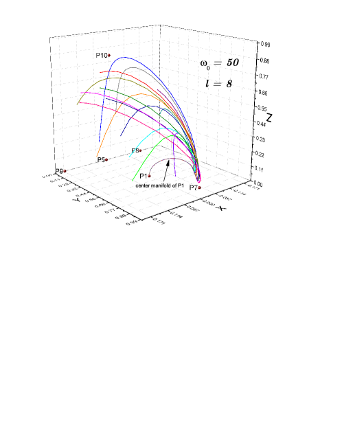
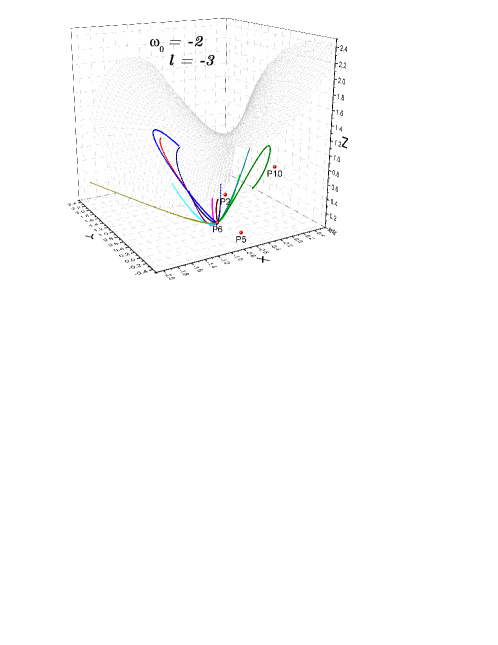
Figure 1: (Color online) Case: $W(\psi)=W_{0}e^{k\psi}$ and $V(\varphi)=V_{0}e^{l\varphi}$. Evolution of some orbits of the dynamical system (35) projected on space $(x,y,z)$ for $\omega_{0}=50,l=8.$ The initial conditions are chosen randomly to show that, irrespectively of the initial conditions, the orbits are attracted by the center manifold of the equilibrium point $P_{1}$.

Figure 2: (Color online) Case: $W(\psi)=W_{0}e^{k\psi}$ and $V(\varphi)=V_{0}e^{l\varphi}$. Evolution of some orbits of the dynamical system (35) projected on space $(x,y,z)$ for $\omega_{0}=-2,l=-3.$ The initial conditions are chosen randomly to show that, irrespectively of the initial conditions, the orbits are attracted by the the equilibrium point $P_{6}$.

Therefore, the local center manifold of the origin can be expressed

$$\left\{(u,v_{1},v_{2},v_{3})\in\mathbb{R}^{4}:v_{1}=0,\right.$$

$$\left.v_{2}=-\frac{\sqrt{2}(l-1)^{2}\left(-\sqrt{3}\left(2\omega_{0}+3\right)\omega_{0}+\sqrt{\left(2\omega_{0}+3\right)\left(-16l+6\omega_{0}+25\right)}\omega_{0}+\sqrt{3}l\left(2\omega_{0}+3\right)\right)u^{2}}{(l+1)^{5/2}\left(2\omega_{0}+3\right)\left(16\sqrt{3}l-\sqrt{3}\left(6\omega_{0}+25\right)-3\sqrt{\left(2\omega_{0}+3\right)\left(-16l+6\omega_{0}+25\right)}\right)},\right.$$

$$\left.v_{3}=-\frac{\sqrt{2}(l-1)^{2}\left(-\sqrt{3}\left(2\omega_{0}+3\right)\omega_{0}-\sqrt{\left(2\omega_{0}+3\right)\left(-16l+6\omega_{0}+25\right)}\omega_{0}+\sqrt{3}l\left(2\omega_{0}+3\right)\right)u^{2}}{(l+1)^{5/2}\left(2\omega_{0}+3\right)\left(16\sqrt{3}l-\sqrt{3}\left(6\omega_{0}+25\right)+3\sqrt{\left(2\omega_{0}+3\right)\left(-16l+6\omega_{0}+25\right)}\right)}\right\}.$$

The dynamics on the center manifold are given by a gradient like equation $u^{\prime}=-\nabla\Pi(u)$, where $\Pi(u)=\frac{(l-1)u^{4}}{8(l+1)^{2}}$, for which the origin is a degenerate local minimum whenever $l>1$ (recall the existence conditions for $P_{1}$ are $2\omega_{0}+3\neq 0,l\geq 1$). This implies that the center manifold of $P_{1}$ is stable when $1<l\leq\frac{1}{16}\left(6\omega_{0}+25\right)$. For $l>\frac{1}{16}\left(6\omega_{0}+25\right)$ the unstable manifold is not empty. Neglecting the order terms $\mathcal{O}(\lambda^{3})$ the center can be given in the original variables by the graph:

$$x=-\frac{(l-1)\lambda^{2}}{\sqrt{6}(l+1)^{2}},\quad y=\frac{\sqrt{2}}{\sqrt{l+1}}-\frac{\left((l-1)\left(l-2\omega_{0}\right)\right)\lambda^{2}}{4\left(\sqrt{2}(l+1)^{5/2}\right)},\quad z=\frac{(l-1)\lambda}{\sqrt{6}(l+1)}.$$ (44a)

In the figure 2 we present some orbits of the dynamical system (35) projected on the space $(x,y,z)$ for $W(\psi)=W_{0}e^{k\psi}$ and $V(\varphi)=V_{0}e^{l\varphi}$ with $\omega_{0}=50$ and $l=8$. The initial conditions were chosen randomly to show that, irrespectively of the initial conditions, the orbits are attracted by the center manifold of the equilibrium point $P_{1}$. Latter on, in Section 5.1 it will be shown that the cosmological solutions represented by these orbits, tends to the solution associated to $P_{1}$. Furthermore, as it is shown in Figure 3, the cosmological parameters behave in accordance with the current cosmological paradigm. This feature makes the model very interesting from the cosmological point of view.

In the Fig. 2 are displayed some orbits of the dynamical system (35) projected on space $(x,y,z)$ for $\omega_{0}=-2,l=-3.$ The initial conditions are chosen randomly to show that, irrespectively of the initial conditions, the orbits are attracted by the equilibrium point $P_{6}$. In this example, the phase space is the interior of a hyperboloid that corresponds to the boundary of the phase space and it is represented by a gray mesh. The late-time attractor is a phantom dominated solution.

As we have commented before, the model studied in Cid:2015pja can be considered as a special case of the model $W(\psi)=W_{0}e^{k\psi}$ and $V(\varphi)=V_{0}e^{l\varphi}$ with
$k=-\lambda_{W},l=1-\lambda_{U}\sqrt{\omega_{0}+\frac{3}{2}},\omega_{0}>-\frac{3}{2}$. In this section, we have investigated the stability of the equilibrium solutions in the dilatonic frame. In the reference Cid:2015pja it was studied the stability of the equilibrium points in both the Jordan and the Einstein frames, so our results complement those found in Cid:2015pja . In particular, we notice that the equilibrium point (in the Jordan frame), named $J_{4}$ in Cid:2015pja corresponds to $P_{1}$ investigated in this section with the identification $\lambda_{U}=(1-l)\gamma,\gamma^{-1}=\sqrt{\omega_{0}+\frac{3}{2}}$, due to it satisfies

$$J_{4}:\left(e^{-\frac{\varphi}{2}}\frac{\dot{\psi}}{\sqrt{6}H},\frac{\dot{\varphi}}{H},\frac{\sqrt{V(\varphi)}}{\sqrt{3}H}\right)=\left(0,0,\frac{\sqrt{2\gamma}}{\sqrt{2\gamma-\lambda_{U}}}\right)=\left(0,0,\frac{\sqrt{2}}{\sqrt{1+l}}\right).$$ (45)

The stability conditions deduced in Cid:2015pja the Jordan’s frame formulation and also in the Einstein’s frame formulation are $\lambda_{U}<0,\gamma>0$. That is, $\omega_{0}>-\frac{3}{2},l>1$. The stability in the dilatonic frame formulation is $1<l\leq\frac{1}{16}\left(6\omega_{0}+25\right)$. They are the equivalent conditions with the identifications $\lambda_{U}=(1-l)\gamma,\gamma^{-1}=\sqrt{\omega_{0}+\frac{3}{2}}$. The equilibrium points $J_{4}$ and $E_{4}$ (the representations of $P_{1}$ in the Jordan’s frame and in the Einstein’s frame, respectively) correspond to an intermediate accelerated solution instead of a de Sitter solution (see derivation in Cid:2015pja ). That is, an attractor in the Jordan frame corresponds to the solution of the form $a(t)\simeq e^{\alpha_{1}t^{p_{1}}}$, as $t\rightarrow\infty$ where $\alpha_{1}>0$ and $0<p_{1}<1$ for a wide range of parameters. Furthermore, when we work in the Einstein frame we get that the attractor is also the solution of the form $\bar{a}(\bar{t})\simeq e^{\alpha_{2}\bar{t}^{p_{2}}}$, as $\bar{t}\rightarrow\infty$ where $\alpha_{2}>0$ and $0<p_{2}<1$, for the same conditions on the parameter space as in the Jordan frame. An equivalent result can be deduced straightforwardly for the dilatonic frame. We proceed as follows. According to the center manifold calculation, we have from (44a), the definition $\lambda:=ke^{-\varphi/2}$, and the definition (28) that (as $\varphi\rightarrow\infty$):

$$\frac{d\varphi}{d\ln a}=-\frac{(l-1)k^{2}e^{-\varphi}}{(l+1)^{2}},\ \frac{d\psi}{d\ln a}=\frac{(l-1)k}{(l+1)},\ \frac{dt}{d\ln a}=\frac{8(l+1)^{2}e^{\varphi}-k^{2}(l-1)(l-2\omega_{0})}{4\sqrt{\frac{2}{3}}(l+1)^{5/2}\sqrt{V_{0}}e^{\frac{(2-l)\varphi}{2}}}.$$ (46a)

With general solution

$$\varphi(a)=\ln\left|c_{1}-\frac{k^{2}(l-1)\ln(a)}{(l+1)^{2}}\right|,\quad\psi(a)=c_{3}+\frac{k(l-1)\ln(a)}{l+1},$$ (47a)

$$t(a)=\frac{\sqrt{\frac{3}{2}}\left|c_{1}-\frac{k^{2}(l-1)\ln(a)}{(l+1)^{2}}\right|{}^{l/2}\left(k^{2}(l-1)(l(l+8\ln(a)+2)-2(l+2)\omega_{0})-8c_{1}l(l+1)^{2}\right)}{2k^{2}(l-1)l\sqrt{l+1}(l+2)\sqrt{V_{0}}}+c_{2},$$ (47b)

where $c_{1},c_{2},c_{3}$ are integration constants. For large $a$, the leading terms are

$$t(a)\simeq\frac{2\sqrt{6}\ln(a)\left|c_{1}-\frac{k^{2}(l-1)\ln(a)}{(l+1)^{2}}\right|{}^{l/2}}{\sqrt{l+1}(l+2)\sqrt{V_{0}}}$$

$$\implies\ln a\simeq t^{\frac{2}{2+l}}\implies a\simeq e^{At^{p}},\quad p:=\frac{2}{2+l},\quad\frac{32}{57+6\omega_{0}}<p<\frac{2}{3},\;\text{as}\;t\rightarrow\infty.$$ (48)

with the identifications $\lambda_{U}=(1-l)\gamma,\gamma^{-1}=\sqrt{\omega_{0}+\frac{3}{2}}$ we obtain the same exponent $p=p_{1}=p_{2}=\frac{2\gamma}{3\gamma-\lambda_{U}}$. Since $p<\frac{2}{3}$, $P_{1}$ is not a de Sitter solution (that requires $p=1$).

4.2 Case: $W(\psi)=W_{0}\psi^{k}$ and $V(\varphi)=V_{0}e^{l\varphi}$

In this example we have $s=-l=\text{const.},\lambda=-\frac{ke^{\varphi/2}}{\psi},\Gamma_{\varphi}=1,\Gamma_{\psi}=\frac{k-1}{k}$. Thus $h(s,\lambda)=\frac{k-1}{k}$. Assuming $k\neq 0$ and introducing $x_{1}=\frac{2\lambda z}{k}+x$ the system (31) becomes

$$x_{1}^{\prime}=\Big{[}-\frac{3(l+1)y^{2}}{2\omega_{0}+3}+\frac{6\lambda^{2}}{k}+z\left(\frac{4\sqrt{6}\omega_{0}\lambda^{3}}{k^{2}}+\frac{12\sqrt{6}\left(2\omega_{0}+1\right)\lambda}{k\left(2\omega_{0}+3\right)}\right)$$

$$+z^{2}\left(\frac{12\omega_{0}\left(2\omega_{0}+1\right)\lambda^{2}}{k^{2}\left(2\omega_{0}+3\right)}+\frac{6\omega_{0}}{2\omega_{0}+3}\right)+\frac{18}{2\omega_{0}+3}-3\Big{]}x_{1}$$

$$+\left[-\frac{\sqrt{6}\omega_{0}\lambda^{2}}{k}-\frac{12z\omega_{0}\left(2\omega_{0}+1\right)\lambda}{k\left(2\omega_{0}+3\right)}-\frac{\sqrt{6}\left(8\omega_{0}+3\right)}{2\omega_{0}+3}\right]x_{1}^{2}$$

$$+\left[3\omega_{0}+\frac{9}{2\omega_{0}+3}-3\right]x_{1}^{3}+y^{2}\left[-\frac{\sqrt{6}\lambda^{2}}{k}-\frac{\sqrt{6}(l+1)}{2\omega_{0}+3}\right]$$

$$+z^{2}\left[-\frac{4\sqrt{6}\omega_{0}\lambda^{4}}{k^{3}}-\frac{\sqrt{6}\left(3(k+2)+2(k+6)\omega_{0}\right)\lambda^{2}}{k^{2}\left(2\omega_{0}+3\right)}-\frac{3\sqrt{6}}{2\omega_{0}+3}\right]$$

$$+z\left[-\frac{12\lambda^{3}}{k^{2}}-\frac{24\lambda}{2\omega_{0}k+3k}\right]+\frac{2\sqrt{6}}{2\omega_{0}+3}+\frac{\sqrt{6}\lambda^{2}}{k},$$ (49a)

$$y^{\prime}=\left[\frac{6}{2\omega_{0}+3}\right]y+\left[\frac{\sqrt{6}\left(3l+2(l-4)\omega_{0}\right)}{4\omega_{0}+6}-\frac{12z\lambda\omega_{0}\left(2\omega_{0}+1\right)}{k\left(2\omega_{0}+3\right)}\right]x_{1}y$$

$$+\left[\left(\frac{12\omega_{0}\left(2\omega_{0}+1\right)\lambda^{2}}{k^{2}\left(2\omega_{0}+3\right)}+\frac{6\omega_{0}}{2\omega_{0}+3}\right)z+\frac{\sqrt{6}\lambda\left(-3l-2(l-4)\omega_{0}\right)}{k\left(2\omega_{0}+3\right)}\right]zy$$

$$-\frac{3(l+1)y^{3}}{2\omega_{0}+3}+\left[3\omega_{0}+\frac{9}{2\omega_{0}+3}-3\right]x_{1}^{2}y,$$ (49b)

$$z^{\prime}=\sqrt{\frac{3}{2}}\lambda+\left[\frac{12\omega_{0}\left(2\omega_{0}+1\right)\lambda^{2}}{k^{2}\left(2\omega_{0}+3\right)}+\frac{6\omega_{0}}{2\omega_{0}+3}\right]z^{3}$$

$$+\left[\frac{\sqrt{\frac{3}{2}}\lambda\left(-3k-2(k-10)\omega_{0}+6\right)}{k\left(2\omega_{0}+3\right)}-\frac{2\sqrt{6}\lambda^{3}\omega_{0}}{k^{2}}\right]z^{2}$$

$$+\left[-\frac{6\lambda^{2}}{k}+\frac{6}{2\omega_{0}+3}-3\right]z+y^{2}\left[-\frac{3(l+1)z}{2\omega_{0}+3}-\sqrt{\frac{3}{2}}\lambda\right]$$

$$+x_{1}^{2}\left[z\left(3\omega_{0}+\frac{9}{2\omega_{0}+3}-3\right)-\sqrt{\frac{3}{2}}\lambda\omega_{0}\right]$$

$$+x_{1}\left[-\frac{12\lambda\omega_{0}\left(2\omega_{0}+1\right)z^{2}}{k\left(2\omega_{0}+3\right)}+\left(\frac{2\sqrt{6}\lambda^{2}\omega_{0}}{k}-\frac{\sqrt{6}\left(10\omega_{0}+3\right)}{4\omega_{0}+6}\right)z+3\lambda\right],$$ (49c)

$$\lambda^{\prime}=\sqrt{\frac{3}{2}}x_{1}\lambda.$$ (49d)

The system is a form-invariant under the change $(y,z,\lambda)\rightarrow(-y,-z,-\lambda)$. Therefore, without losing generality we can investigate just the sector $y\geq 0,z\geq 0,\lambda\geq 0$. Henceforth, we will focus on the stability properties of the system (49) for the state vector $(x,y,z,\lambda)$ defined in the phase space

$$\Big{\{}(x_{1},y,z,\lambda)\in\mathbb{R}^{4}:y\geq 0,z\geq 0,\lambda\geq 0,2\omega_{0}+3\neq 0,k\left(k\left(-\sqrt{6}x_{1}+y^{2}+z^{2}-1\right)+2\sqrt{6}\lambda z\right)$$

$$+\omega_{0}(kx_{1}-2\lambda z)^{2}\leq 0\Big{\}}.$$ (50)

We will focus on the study of the particular choice of potentials (15):

$$V\left(\varphi\right)=V_{0}e^{\left(\beta-1\right)\varphi}~{}\ ,~{}W\left(\psi\right)=W_{0}\psi^{2\beta},$$ (51)

that lead to Noether pointlike symmetries, corresponding to the choice $l=\beta-1$, and $k=2\beta$. The equilibrium points are the following

1. $:=(x_{1},y,z,\lambda)=\left(0,\frac{\sqrt{2}}{\sqrt{\beta}},0,0\right)$.
   The eigenvalues are
   $\Big{\{}0,-3,-\frac{\sqrt{3}\sqrt{\left(2\omega_{0}+3\right)\left(-16\beta+6\omega_{0}+41\right)}}{4\omega_{0}+6}-\frac{3}{2},\frac{1}{2}\left(\frac{\sqrt{3}\sqrt{\left(2\omega_{0}+3\right)\left(-16\beta+6\omega_{0}+41\right)}}{2\omega_{0}+3}-3\right)\Big{\}}$.
   The stable manifold is three dimensional for $\beta>2,\omega_{0}\geq\frac{1}{6}(16\beta-41)$.

2. $:=(x_{1},y,z,\lambda)=\left(-\sqrt{\frac{2}{3}},0,\sqrt{-\frac{2\omega_{0}}{3}-1},0\right)$. The eigenvalues are
   $\{-1,1,6,3-\beta\}$.
   It is a saddle point with a three dimensional unstable manifold for $\beta<3$.

3. $:=(x_{1},y,z,\lambda)=\left(-\frac{\sqrt{6}}{\beta},-\frac{\sqrt{3-\beta}}{\beta},-\frac{\sqrt{(\beta-5)\beta-6\omega_{0}-3}}{\beta},0\right)$.
   The eigenvalues are $\Big{\{}-\frac{3}{\beta},6,\frac{3}{2\beta}-\frac{\sqrt{6(25-8\beta)\omega_{0}+8(\beta-6)(\beta-2)\beta+81}}{2\beta\sqrt{\frac{2\omega_{0}}{3}+1}}$,
   $\frac{3}{2\beta}+\frac{\sqrt{6(25-8\beta)\omega_{0}+8(\beta-6)(\beta-2)\beta+81}}{2\beta\sqrt{\frac{2\omega_{0}}{3}+1}}\Big{\}}$.
   It is a saddle.

4. $:=(x_{1},y,z,\lambda)=\left(-\frac{\sqrt{6}}{\beta},\frac{\sqrt{3-\beta}}{\beta},\frac{\sqrt{(\beta-5)\beta-6\omega_{0}-3}}{\beta},0\right)$.
   The eigenvalues are $\Big{\{}-\frac{3}{\beta},6,\frac{3}{2\beta}-\frac{\sqrt{6(25-8\beta)\omega_{0}+8(\beta-6)(\beta-2)\beta+81}}{2\beta\sqrt{\frac{2\omega_{0}}{3}+1}}$,
   $\frac{3}{2\beta}+\frac{\sqrt{6(25-8\beta)\omega_{0}+8(\beta-6)(\beta-2)\beta+81}}{2\beta\sqrt{\frac{2\omega_{0}}{3}+1}}\Big{\}}$.
   It is a saddle.

5. $:=(x_{1},y,z,\lambda)=\left(\frac{2\sqrt{\frac{2}{3}}}{2\omega_{0}+1},0,0,0\right)$.
   The eigenvalues are $\left\{\frac{2}{2\omega_{0}+1},\frac{2\beta}{2\omega_{0}+1},-3,-\frac{6\omega_{0}+5}{2\omega_{0}+1}\right\}$.
   It is a sink for $\beta>0,\omega_{0}<-\frac{3}{2}$.

6. $:=(x_{1},y,z,\lambda)$
   $=\left(-\frac{\sqrt{\frac{2}{3}}(\beta-2)}{\beta+2\omega_{0}+1},-\frac{\sqrt{\left(2\omega_{0}+3\right)\left(2\omega_{0}-\frac{1}{3}(\beta-5)(\beta+1)\right)}}{\beta+2\omega_{0}+1},0,0\right)$.
   The eigenvalues are
   $\left\{-\frac{\beta-2}{\beta+2\omega_{0}+1},\frac{2(\beta-2)\beta}{\beta+2\omega_{0}+1},\frac{\beta^{2}-5\beta-6\omega_{0}-3}{\beta+2\omega_{0}+1},\frac{\beta^{2}-4\beta-6\omega_{0}-5}{\beta+2\omega_{0}+1}\right\}$.
   It is a sink for $\beta<0,\omega_{0}<-\frac{3}{2}$. It is a saddle otherwise.

7. $:=(x_{1},y,z,\lambda)$
   $=\left(-\frac{\sqrt{\frac{2}{3}}(\beta-2)}{\beta+2\omega_{0}+1},\frac{\sqrt{\left(2\omega_{0}+3\right)\left(2\omega_{0}-\frac{1}{3}(\beta-5)(\beta+1)\right)}}{\beta+2\omega_{0}+1},0,0\right)$.
   The eigenvalues are
   $\left\{-\frac{\beta-2}{\beta+2\omega_{0}+1},\frac{2(\beta-2)\beta}{\beta+2\omega_{0}+1},\frac{\beta^{2}-5\beta-6\omega_{0}-3}{\beta+2\omega_{0}+1},\frac{\beta^{2}-4\beta-6\omega_{0}-5}{\beta+2\omega_{0}+1}\right\}$.
   It is a saddle.

8. $:=(x_{1},y,z,\lambda)=\left(\frac{\sqrt{3}-\sqrt{2\omega_{0}+3}}{\sqrt{2}\omega_{0}},0,0,0\right)$.
   The eigenvalues are
   $\Big{\{}-\frac{\sqrt{6\omega_{0}+9}-3}{2\omega_{0}},-\frac{\sqrt{6\omega_{0}+9}-3}{2\omega_{0}},\frac{6\omega_{0}-\sqrt{6\omega_{0}+9}+3}{\omega_{0}},\frac{6\omega_{0}-(\beta+1)\left(\sqrt{6\omega_{0}+9}-3\right)}{2\omega_{0}}\Big{\}}$.
   It is a saddle.

9. $:=(x_{1},y,z,\lambda)=\left(\frac{\sqrt{3}+\sqrt{2\omega_{0}+3}}{\sqrt{2}\omega_{0}},0,0,0\right)$.
   The eigenvalues are $\Big{\{}\frac{\sqrt{6\omega_{0}+9}+3}{2\omega_{0}},\frac{\sqrt{6\omega_{0}+9}+3}{2\omega_{0}},\frac{6\omega_{0}+\sqrt{6\omega_{0}+9}+3}{\omega_{0}}$,
   $\frac{(\beta+1)\left(\sqrt{6\omega_{0}+9}+3\right)+6\omega_{0}}{2\omega_{0}}\Big{\}}$.
   It is a sink for

   1. $-1<\beta\leq 0,\frac{1}{6}(\beta-5)(\beta+1)<\omega_{0}<0$, or

   2. $\beta>0,-\frac{5}{6}<\omega_{0}<0$.

   It is a source for

   1. $\beta\leq-1,\omega_{0}>\frac{1}{6}(\beta-5)(\beta+1)$, or

   2. $\beta>-1,\omega_{0}>0$.

   It is a saddle otherwise.

10. $:=(x_{1},y,z,\lambda)=\Big{(}0,-\frac{\sqrt{2\lambda^{2}\omega_{0}\left((14-(\beta-4)\beta)\lambda^{2}+6\beta(\beta+2)+6\lambda^{2}\omega_{0}\right)-3\left((\beta-5)\lambda^{2}-4\beta\right)\left(2\beta^{2}+(\beta+1)\lambda^{2}\right)}}{\sqrt{3}\left(2\beta^{2}+(\beta+1)\lambda^{2}+2\lambda^{2}\omega_{0}\right)}$,
    $\frac{\sqrt{\frac{2}{3}}(\beta-2)\beta\lambda}{2\beta^{2}+(\beta+1)\lambda^{2}+2\lambda^{2}\omega_{0}},\lambda\Big{)}$. The eigenvalues and the nature of the equilibrium points has to be handled for specific choices of the parameters in the region of existence.

11. $:=(x_{1},y,z,\lambda)=\Big{(}0,\frac{\sqrt{2\lambda^{2}\omega_{0}\left((14-(\beta-4)\beta)\lambda^{2}+6\beta(\beta+2)+6\lambda^{2}\omega_{0}\right)-3\left((\beta-5)\lambda^{2}-4\beta\right)\left(2\beta^{2}+(\beta+1)\lambda^{2}\right)}}{\sqrt{3}\left(2\beta^{2}+(\beta+1)\lambda^{2}+2\lambda^{2}\omega_{0}\right)}$,
    $\frac{\sqrt{\frac{2}{3}}(\beta-2)\beta\lambda}{2\beta^{2}+(\beta+1)\lambda^{2}+2\lambda^{2}\omega_{0}},\lambda\Big{)}$. The eigenvalues and the nature of the equilibrium points have to be handled for specific choices of the parameters in the region of existence.

12. $:=(x_{1},y,z,\lambda)=\left(0,0,\sqrt{-\frac{2\omega_{0}}{3}-1},\frac{\beta}{\sqrt{-\omega_{0}-\frac{3}{2}}}\right)$.
    The eigenvalues are $\{3-\beta,1,-2(\beta-3),1\}$.
    It is a source for

    1. $\omega_{0}\in\mathbb{R},\beta=0$, or

    2. $0<\beta<3,\omega_{0}<-\frac{3}{2}$.

13. $:=(x_{1},y,z,\lambda)={\left(0,0,\frac{1}{96\beta^{2}\sqrt{(-10+2\beta)(2+2\beta)-24\omega_{0}}\omega_{0}\sqrt{3+2\omega_{0}}}\right.}\newline {\left(-48\sqrt{3}\omega_{0}^{2}+3(2+2\beta)\left(-2\sqrt{3}+2\sqrt{3}\beta+\sqrt{3(-2+2\beta)^{2}+8\omega_{0}\left(6+2\beta+6\omega_{0}\right)}\right)+\right.}\newline {\left.4\omega_{0}\left(\sqrt{3}(-6+2\beta)(2+2\beta)+3\sqrt{3(-2+2\beta)^{2}+8\omega_{0}\left(6+2\beta+6\omega_{0}\right)}\right)\right)}\newline {\surd(-6\beta(-8+2\beta(-14+2\beta))+}\newline {\left.2\beta\left(12(4+2\beta)\omega_{0}-(-4+2\beta)\sqrt{9(-2+2\beta)^{2}+24\omega_{0}\left(6+2\beta+6\omega_{0}\right)}\right)\right),}\newline {\left.\left(8\sqrt{3}\beta^{3/2}\right)\right/(\surd(6\beta(-8+2\beta(-14+2\beta))-}\newline {\left.\left.\left.2\beta\left(12(4+2\beta)\omega_{0}+(-4+2\beta)\sqrt{9(-2+2\beta)^{2}+24\omega_{0}\left(6+2\beta+6\omega_{0}\right)}\right)\right)\right)\right)}$. The eigenvalues and the nature of the equilibrium points have to be handled for specific choices of the parameters in the region of existence.

14. $:=(x_{1},y,z,\lambda)={\left(0,0,\frac{1}{96\beta^{2}\sqrt{(-10+2\beta)(2+2\beta)-24\omega_{0}}\omega_{0}\sqrt{3+2\omega_{0}}}\right.}\newline {\left(-48\sqrt{3}\omega_{0}^{2}+4\omega_{0}\left(\sqrt{3}(-6+2\beta)(2+2\beta)-3\sqrt{3(-2+2\beta)^{2}+8\omega_{0}\left(6+2\beta+6\omega_{0}\right)}\right)+\right.}\newline {\left.3(2+2\beta)\left(-2\sqrt{3}+2\sqrt{3}\beta-\sqrt{3(-2+2\beta)^{2}+8\omega_{0}\left(6+2\beta+6\omega_{0}\right)}\right)\right)}\newline {\surd(-6\beta(-8+2\beta(-14+2\beta))+}\newline {\left.2\beta\left(12(4+2\beta)\omega_{0}+(-4+2\beta)\sqrt{9(-2+2\beta)^{2}+24\omega_{0}\left(6+2\beta+6\omega_{0}\right)}\right)\right),}\newline {\left.\left(8\sqrt{3}\beta^{3/2}\right)\right/(\surd(6\beta(-8+2\beta(-14+2\beta))+}\newline {\left.\left.\left.2\beta\left(-12(4+2\beta)\omega_{0}+(-4+2\beta)\sqrt{9(-2+2\beta)^{2}+24\omega_{0}\left(6+2\beta+6\omega_{0}\right)}\right)\right)\right)\right)}$. The eigenvalues and the nature of the equilibrium points have to be handled for specific choices of the parameters in the region of existence.

4.2.1 Center manifold of $P_{1}$.

From the previous linear analysis we found that the equilibrium point $P_{1}$ is nonhyperbolic with a three dimensional stable manifold provided $\beta>2,\omega_{0}\geq\frac{1}{6}(16\beta-41)$.

Introducing the new variables

$$u=\lambda,$$

$$v_{1}=z-\frac{(\beta-2)\lambda}{\sqrt{6}\beta}$$

$$v_{2}=-\frac{x\left(4(\beta-5)\omega_{0}+6(\beta-1)\right)}{2\sqrt{\beta}\sqrt{\left(2\omega_{0}+3\right)\left(-16\beta+6\omega_{0}+41\right)}}$$

$$+\frac{\left(\sqrt{\left(2\omega_{0}+3\right)\left(-16\beta+6\omega_{0}+41\right)}-2\sqrt{3}\omega_{0}+5\sqrt{3}\right)\left(y-\frac{\sqrt{2}}{\sqrt{\beta}}\right)}{2\sqrt{\left(2\omega_{0}+3\right)\left(-16\beta+6\omega_{0}+41\right)}},$$

$$v_{3}=\frac{x\left(4(\beta-5)\omega_{0}+6(\beta-1)\right)}{2\sqrt{\beta}\sqrt{\left(2\omega_{0}+3\right)\left(-16\beta+6\omega_{0}+41\right)}}$$

$$+\frac{\left(\sqrt{\left(2\omega_{0}+3\right)\left(-16\beta+6\omega_{0}+41\right)}+2\sqrt{3}\omega_{0}-5\sqrt{3}\right)\left(y-\frac{\sqrt{2}}{\sqrt{\beta}}\right)}{2\sqrt{\left(2\omega_{0}+3\right)\left(-16\beta+6\omega_{0}+41\right)}},$$

we obtain the evolution equations

$$u^{\prime}=-\frac{\sqrt{\beta}uv_{2}\left(\sqrt{3}\sqrt{(2\omega_{0}+3)(-16\beta+6\omega_{0}+41)}+6\omega_{0}-15\right)}{2\sqrt{2}(2(\beta-5)\omega_{0}+3(\beta-1))}+$$

$$\frac{\sqrt{\beta}uv_{3}\left(\sqrt{3}\sqrt{(2\omega_{0}+3)(-16\beta+6\omega_{0}+41)}-6\omega_{0}+15\right)}{2\sqrt{2}(2(\beta-5)\omega_{0}+3(\beta-1))},$$ (52a)

$$v_{1}^{\prime}=-3v_{1}+\mathcal{O}(2),$$ (52b)

$$v_{2}^{\prime}=-\frac{v_{2}\left(\sqrt{3}\sqrt{(2\omega_{0}+3)(-16\beta+6\omega_{0}+41)}+6\omega_{0}+9\right)}{4\omega_{0}+6}+\mathcal{O}(2),$$ (52c)

$$v_{3}^{\prime}=\frac{v_{3}\left(\sqrt{3}\sqrt{(2\omega_{0}+3)(-16\beta+6\omega_{0}+41)}-6\omega_{0}-9\right)}{4\omega_{0}+6}+\mathcal{O}(2).$$ (52d)

The system (52) can be diagonalized as

$$u^{\prime} =Cu+f\left(u,\mathbf{v}\right),$$

$$\mathbf{v}^{\prime} =P\mathbf{v}+\mathbf{g}\left(u,\mathbf{v}\right),$$ (53)

where $\left(u,\mathbf{v}\right)\in\mathbb{R}\times\mathbb{R}^{3},$ $C\equiv 0\in\mathbb{R}^{1\times 1}$, $P\in\mathbb{R}^{3\times 3}$ has negative eigenvalues, and $f(0)=0,\quad\mathbf{g}(\mathbf{0})=\mathbf{0}$, $f^{\prime}(0)=0,\quad D\mathbf{g}(\mathbf{0})=\mathbf{0}$. Using the center manifold theorem we have that there exists a 1-dimensional invariant local center manifold $W^{c}\left(\mathbf{0}\right)$ of (53) tangent to the center subspace $\mathbf{v}=\mathbf{0}$ at $\mathbf{0}.$ Moreover, $W^{c}\left(\mathbf{0}\right)$ can be represented as

$$W^{c}\left(\mathbf{0}\right)=\Big{\{}\left(u,\mathbf{v}\right)\in\mathbb{R}\times\mathbb{R}^{3}:\mathbf{v}=\mathbf{h}\left(u\right),\mathbf{h}\left(0\right)=\mathbf{0},D\mathbf{h}\left(0\right)=\mathbf{0},\;\left|u\right|<\delta\Big{\}},$$ (54)

for $\delta$ small enough. The dynamics over the center manifold is given by the equation

$$u^{\prime}=f\left(u,\mathbf{h}\left(u\right)\right),$$ (55)

where the function $\mathbf{h}\left(u\right)$ defines the local center manifold and satisfies

$$D\mathbf{h}\left(u\right)\left[f\left(u,\mathbf{h}\left(u\right)\right)\right]-P\mathbf{h}\left(u\right)-\mathbf{g}\left(u,\mathbf{h}\left(u\right)\right)=0.$$

Following the same implemented procedure in section 4.1.1 we obtain

$$\mathbf{h}\left(u\right):=\left[\begin{array}[c]{c}h_{1}\left(u\right)\\ h_{2}\left(u\right)\\ h_{3}\left(u\right)\end{array}\right]=\left[\begin{array}[c]{c}a_{1}u^{2}+\mathcal{O}\left(u^{3}\right)\\ a_{2}u^{2}+\mathcal{O}\left(u^{3}\right)\\ a_{3}u^{2}+\mathcal{O}\left(u^{3}\right)\end{array}\right]$$

where $a_{1}=0$,

$$a_{2}=\frac{\sqrt{2}(\beta-2)^{2}\left(\omega_{0}\sqrt{(2\omega_{0}+3)(-16\beta+6\omega_{0}+41)}+\sqrt{3}\beta(2\omega_{0}+3)-\sqrt{3}(\omega_{0}+1)(2\omega_{0}+3)\right)}{\beta^{5/2}(2\omega_{0}+3)\left(3\sqrt{(2\omega_{0}+3)(-(16\beta-6\omega_{0}-41))}-16\sqrt{3}\beta+\sqrt{3}(6\omega_{0}+41)\right)},$$

$$a_{3}=\frac{\sqrt{2}(\beta-2)^{2}\left(\omega_{0}\left(-\sqrt{(2\omega_{0}+3)(-16\beta+6\omega_{0}+41)}\right)+\sqrt{3}\beta(2\omega_{0}+3)-\sqrt{3}(\omega_{0}+1)(2\omega_{0}+3)\right)}{\beta^{5/2}(2\omega_{0}+3)\left(-3\sqrt{(2\omega_{0}+3)(-(16\beta-6\omega_{0}-41))}-16\sqrt{3}\beta+\sqrt{3}(6\omega_{0}+41)\right)}.$$

Therefore, the dynamics on the center manifold is given by the gradient-like equation

$$u^{\prime}=-\frac{(\beta-2)u^{3}}{2\beta^{2}}=-\frac{d}{du}\left[\frac{(\beta-2)u^{4}}{8\beta^{2}}\right],$$

under the potential $\Pi(u)=\frac{(\beta-2)u^{4}}{8\beta^{2}}$, for which the origin is a degenerate local minimum whenever $\beta>2$ (recall the existence conditions for $P_{1}$ are $\beta>2,\omega_{0}\geq\frac{1}{6}(16\beta-41)$), and under these conditions, the center manifold of $P_{1}$ is stable. In the original variables (28) the center manifold can be locally expressed as the graph

$$x=-\frac{(\beta-2)u^{2}}{\sqrt{6}\beta^{2}},$$ (56a)

$$y=-\frac{(\beta-2)u^{2}(\beta-2\omega_{0}-1)-8\beta^{2}}{4\sqrt{2}\beta^{5/2}},$$ (56b)

$$z=\frac{(\beta-2)u}{\sqrt{6}\beta},$$ (56c)

$$\lambda=u.$$ (56d)

According to the center manifold calculation, we have from (44a), the definition $\lambda:=-\frac{2\beta}{\psi}e^{-\varphi/2}$, and the definition (28), and introducing the time rescaling $\frac{df}{d\tau}=\psi^{2}\frac{df}{d\ln a}$ we have that (as $\lambda\rightarrow 0$):

$$\frac{d\varphi}{d\tau}={4(2-\beta)e^{-\varphi}},$$ (57a)

$$\frac{d\psi}{d\tau}={2(2-\beta)}{\psi},$$ (57b)

$$\frac{dt}{d\tau}=\frac{\sqrt{\frac{3}{2}}e^{-\frac{1}{2}(\beta+1)\varphi}\left(2\psi^{2}e^{\phi}-(\beta-2)(\beta-2\omega_{0}-1)\right)}{\sqrt{\beta}\sqrt{V_{0}}}.$$ (57c)

Integrating the equations, and using the first integral $\ln\left[\frac{a}{a_{0}}\right]=\int\psi^{2}d\tau$ we have the general solution

$$\varphi(\tau)=\ln\left|c_{1}-4(\beta-2)\tau\right|,$$ (58a)

$$\psi(\tau)=c_{2}e^{-2(\beta-2)\tau},$$ (58b)

$$a=a_{0}\exp\left[-\frac{c_{2}^{2}e^{-4(\beta-2)\tau}}{4(\beta-2)}\right],$$ (58c)

$$t-t_{0}=\frac{\sqrt{\frac{3}{2}}\int\left|c_{1}-4(\beta-2)\tau\right|{}^{\frac{1}{2}(-\beta-1)}\left((2-\beta)(\beta-2\omega_{0}-1)+2c_{2}^{2}e^{-4(\beta-2)\tau}\left|c_{1}-4(\beta-2)\tau\right|\right)\,d\tau}{\sqrt{\beta}\sqrt{V_{0}}}$$

$$\simeq-\frac{\sqrt{\frac{3}{2}}(\beta-2\omega_{0}-1)\left|-4\beta\tau+c_{1}+8\tau\right|{}^{\frac{1}{2}-\frac{\beta}{2}}}{2(\beta-1)\sqrt{\beta}\sqrt{V_{0}}}\;\text{for large}\;\tau.$$ (58d)

5 Cosmological consequences

Considering the equations written in the dilatonic frame: (9a),(9b), (9c), and (9d), we can define the following observable quantities:

$${\Omega_{1}}\equiv e^{-\varphi}\frac{{\rho_{1}}}{3H^{2}},\;\text{where}\;{\rho_{1}}:=e^{\varphi}\left(\frac{\omega_{0}\dot{\varphi}^{2}}{2}-3H\dot{\varphi}+V(\varphi)\right),$$ (59a)

$${\Omega_{2}}\equiv e^{-\varphi}\frac{\rho_{2}}{3H^{2}},\;\text{where}\;{\rho_{2}}:=\frac{1}{2}{\dot{\psi}}^{2}+W(\psi),$$ (59b)

$${w_{1}}\equiv\frac{{p_{1}}}{{\rho_{1}}},\;\text{where}\;{p_{1}}:=\frac{4\left(3-2\omega_{0}\right)He^{\varphi}\dot{\varphi}}{4\omega_{0}+6}+\frac{12H^{2}e^{\varphi}}{2\omega_{0}+3}$$

$$-\frac{e^{\varphi}\left(4V^{\prime}(\varphi)+2\left(2\omega_{0}+5\right)V(\varphi)+\left(1-2\omega_{0}\right)\omega_{0}\dot{\phi}^{2}\right)+6\dot{\psi}^{2}}{4\omega_{0}+6},$$ (59c)

$$w_{2}=w_{\psi}\equiv\frac{p_{2}}{\rho_{2}},\;\text{where}\;p_{2}:=\frac{1}{2}{\dot{\psi}}^{2}-W(\psi),\;\text{and}\;$$ (59d)

$${w_{\text{tot}}}:=\frac{{p_{1}}+{p_{2}}}{{\rho_{1}}+{\rho_{2}}}.$$ (59e)

These cosmological parameters can be written in terms of the phase space variables expressed as

$${\Omega_{1}}=x^{2}\omega_{0}-\sqrt{6}x+y^{2},$$ (60a)

$${\Omega_{2}}=-x^{2}\omega_{0}+\sqrt{6}x-y^{2}+1,$$ (60b)

$${w_{1}}=\frac{3\left((2s-5)y^{2}-2\omega_{0}y^{2}-6z^{2}+4\right)+3x^{2}\omega_{0}\left(2\omega_{0}-1\right)+2\sqrt{6}x\left(3-2\omega_{0}\right)}{3\left(2\omega_{0}+3\right)\left(x^{2}\omega_{0}-\sqrt{6}x+y^{2}\right)},$$ (60c)

$${w_{2}}=\frac{x^{2}\omega_{0}-\sqrt{6}x+y^{2}+2z^{2}-1}{x^{2}\left(-\omega_{0}\right)+\sqrt{6}x-y^{2}+1},$$ (60d)

$${w_{\text{tot}}}=\frac{6(s-1)y^{2}+2\omega_{0}\left(6x^{2}\omega_{0}+3x^{2}-5\sqrt{6}x+6z^{2}-3\right)-3\sqrt{6}x+3}{6\omega_{0}+9}.$$ (60e)

$w_{\text{tot}}$ is related to the deceleration for isotropic metrics by $q=\frac{1}{2}(1+3w_{\text{tot}})$.

We continue with the discussion for the interpretations of the model for the choices studied in sections: 4.1, and 4.2. We finish the section with a discussion of the generic features of the models.

5.1 Case: $W(\psi)=W_{0}e^{k\psi}$ and $V(\varphi)=V_{0}e^{l\varphi}$

Table 2: Cosmological parameters corresponding to the formulation in the dilatonic frame as given by Eqs. (9) for $W(\psi)=W_{0}e^{k\psi}$ and $V(\varphi)=V_{0}e^{l\varphi}$.

Equil.	$\Omega_{2}$	$w_{1}$	$w_{2}$	${w_{\text{tot}}}$
Points
$P_{1}$	$\frac{(l-1)}{l+1}$	$-1$	$-1$	$-1$
$P_{2}$	$-\frac{2\omega_{0}}{3}-1$	$1$	$1$	$1$
$P_{3}$	$\frac{\left((l-3)l-6\omega_{0}-7\right)}{(l+1)^{2}}$	$1$	$1$	$1$
$P_{4}$	$\frac{\left((l-3)l-6\omega_{0}-7\right)}{(l+1)^{2}}$	$1$	$1$	$1$
$P_{5}$	$\frac{\left(2\omega_{0}+3\right)\left(6\omega_{0}+5\right)}{3\left(2\omega_{0}+1\right){}^{2}}$	$-1$	$-1$	$-1$
$P_{6}$	$0$	$\frac{2\left(l^{2}-1\right)}{3\left(l+2\omega_{0}+2\right)}-1$	Indeterminate	$\frac{2\left(l^{2}-1\right)}{3\left(l+2\omega_{0}+2\right)}-1$
$P_{7}$	$0$	$\frac{2\left(l^{2}-1\right)}{3\left(l+2\omega_{0}+2\right)}-1$	Indeterminate	$\frac{2\left(l^{2}-1\right)}{3\left(l+2\omega_{0}+2\right)}-1$
$P_{8}$	$0$	$\frac{3\omega_{0}-\sqrt{6\omega_{0}+9}+3}{3\omega_{0}}$	$-1$	$\frac{3\omega_{0}-\sqrt{6\omega_{0}+9}+3}{3\omega_{0}}$
$P_{9}$	$0$	$\frac{3\omega_{0}+\sqrt{6\omega_{0}+9}+3}{3\omega_{0}}$	$-1$	$\frac{3\omega_{0}+\sqrt{6\omega_{0}+9}+3}{3\omega_{0}}$
$P_{10}$	$1$	Indeterminate	$\frac{1}{3}$	$\frac{1}{3}$

In Table 2 we present the cosmological parameters corresponding to the formulation in the dilatonic frame as given by Eqs. (9) for $W(\psi)=W_{0}e^{k\psi}$ and $V(\varphi)=V_{0}e^{l\varphi}$. We have the following results:

• $P_{1}$ satisfies $\Omega_{2}=1-\Omega_{1}=\frac{(l-1)}{l+1}$ with $w_{1}=-1$, $w_{2}=-1$ and ${w_{\text{tot}}}=-1$. Both energy densities $\Omega_{1},\Omega_{2}$ are in the same order of magnitude, that is a scaling solution. We have proved that its center manifold is stable for $1<l\leq\frac{1}{16}\left(6\omega_{0}+25\right)$. Hence, this point is a late-time attractor.

• The equilibrium points $P_{2},P_{3}$ and $P_{4}$ satisfy $w_{1}=1$, $w_{2}=1$, ${w_{\text{tot}}}=1$. That is, they represent stiff solutions. The three solutions are saddle therefore they are not relevant for the late-time cosmology, neither for the early-time cosmology.

• The equilibrium point $P_{5}$, which exists $\omega_{0}<-\frac{3}{2}$ or $-\frac{5}{6}\leq\omega_{0}<-\frac{1}{2}$ or $\omega_{0}>-\frac{1}{2}$, satisfies $\Omega_{2}=\frac{\left(2\omega_{0}+3\right)\left(6\omega_{0}+5\right)}{3\left(2\omega_{0}+1\right){}^{2}}$, $w_{1}=-1$, $w_{2}=-1$ and ${w_{\text{tot}}}=-1$. Both energy densities $\Omega_{1},\Omega_{2}$ are of the same order of magnitude, that is a scaling solution. It is a sink for $l>-1,\omega_{0}<-\frac{3}{2}$ or a saddle otherwise.

• The equilibrium point $P_{6}$, which exists for $l<-2,\omega_{0}=\frac{1}{6}(l-4)(l+2)$ or $l>1,\omega_{0}=\frac{1}{6}(l-4)(l+2)$ or $-2<l<1,\frac{1}{6}(l-4)(l+2)\leq\omega_{0}<\frac{1}{2}(-l-2)$ or $l\leq 1,\omega_{0}<-\frac{3}{2}$ or $l>1,\omega_{0}<\frac{1}{2}(-l-2)$, satisfies $\Omega_{2}=0$, that is, the energy density of the dilatonic field is dominant and the energy density of the quintessence field is negligible. Furthermore, $w_{1}=\frac{2\left(l^{2}-1\right)}{3\left(l+2\omega_{0}+2\right)}-1$ and ${w_{\text{tot}}}=\frac{2\left(l^{2}-1\right)}{3\left(l+2\omega_{0}+2\right)}-1$. That is, according to whether ${w_{\text{tot}}}<-1,{w_{\text{tot}}}=-1$ or $-1<{w_{\text{tot}}}<-\frac{1}{3}$ it represents a phantom solution, a solution with $w_{\text{tot}}=-1$ or a quintessence solution. It is a sink for $l<-1,\omega_{0}<-\frac{3}{2}$. It is a saddle otherwise.

• The equilibrium point $P_{7}$ exists for $l>1,\omega_{0}\geq\frac{1}{6}(l-4)(l+2)$ or $l<-2,\omega_{0}\geq\frac{1}{6}(l-4)(l+2)$ or $l=-2,\omega_{0}>0$ or $l=1,\omega_{0}>-\frac{3}{2}$ or $-2<l<1,\omega_{0}>\frac{1}{2}(-l-2)$ or $l>1,\frac{1}{2}(-l-2)<\omega_{0}<-\frac{3}{2}$ or $-2<l<1,\omega_{0}=\frac{1}{6}(l-4)(l+2)$. The cosmological observables are $\Omega_{2}=0$, $w_{1}=\frac{2\left(l^{2}-1\right)}{3\left(l+2\omega_{0}+2\right)}-1$ and ${w_{\text{tot}}}=\frac{2\left(l^{2}-1\right)}{3\left(l+2\omega_{0}+2\right)}-1$. It is a saddle, therefore they are not relevant for the late-time cosmology, neither for the early-time cosmology.

• The equilibrium point $P_{8}$, which exists for $\omega_{0}>-\frac{3}{2},\omega_{0}\neq 0$, satisfies $\Omega_{2}=0$ that is, the energy density of the dilatonic field is dominant and the energy density of the quintessence field is negligible. Furthermore,
  $w_{1}=\frac{3\omega_{0}-\sqrt{6\omega_{0}+9}+3}{3\omega_{0}}$, $w_{2}=-1$, and $w_{\text{tot}}=\frac{3\omega_{0}-\sqrt{6\omega_{0}+9}+3}{3\omega_{0}}$. The total energy density represents a standard matter source with $0<w_{\text{tot}}<1$. It is a saddle. Therefore, they are not relevant for the late-time cosmology neither for the early-time cosmology.

• The equilibrium point $P_{9}$, which exists for $\omega_{0}>-\frac{3}{2},\omega_{0}\neq 0$, satisfies $\Omega_{2}=0$ that is, the energy density of the dilatonic field is dominant and the energy density of the quintessence field is negligible. Furthermore,
  $w_{1}=\frac{3\omega_{0}+\sqrt{6\omega_{0}+9}+3}{3\omega_{0}}$, $w_{2}=-1$, and $w_{\text{tot}}=\frac{3\omega_{0}+\sqrt{6\omega_{0}+9}+3}{3\omega_{0}}$. That is, the second fluid behaves as a cosmological constant whereas the effective equation of state (of the total cosmic budget) is that of quintessence field for $-\frac{9}{8}<\omega_{0}<-\frac{5}{6}$, a cosmological constant for $\omega_{0}=-\frac{5}{6}$ and the phantom field for $-\frac{5}{6}<\omega_{0}<0$. It is a sink for $-2<l\leq-1,\frac{1}{6}(l-4)(l+2)<\omega_{0}<0$, or $l>-1,-\frac{5}{6}<\omega_{0}<0$ (in both cases it is a phantom attractor). It is a source for $l\leq-2,\omega_{0}>\frac{1}{6}(l-4)(l+2)$, or $l>-2,\omega_{0}>0$ (and then, it behaves as a standard matter source ). It is a saddle otherwise.

• The equilibrium point $P_{10}$ satisfies $\Omega_{2}=1$. That is dominated by the quintessence field and the contribution of the dilatonic field to the total energy density is negligible. It satisfies $w_{2}=\frac{1}{3}$ and ${w_{\text{tot}}}=\frac{1}{3}$. This means that the corresponding cosmological solution mimics radiation. Interestingly, it is a saddle with a three dimensional stable manifold provided $\omega_{0}\geq\frac{45}{2}$.

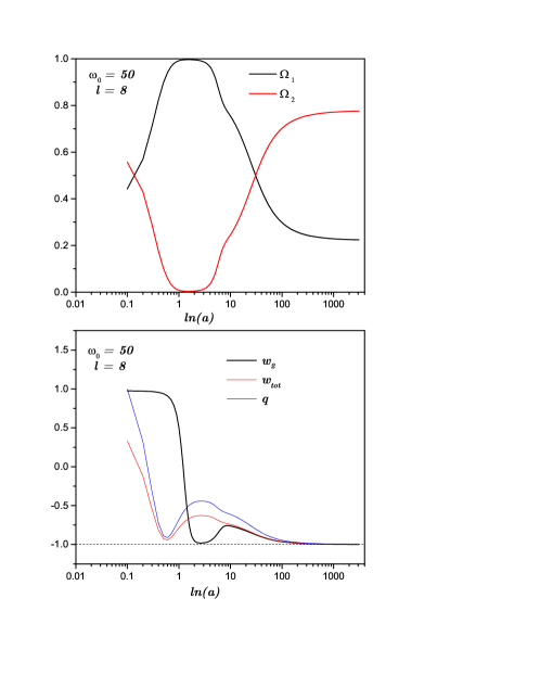
Figure 3: Qualitative evolution of the dimensionless energy densities $\Omega_{1},\Omega_{2}$ and the observables $w_{2},{w_{\text{tot}}},q$ vs $\ln(a)$ for $W(\psi)=W_{0}e^{k\psi}$ and $V(\varphi)=V_{0}e^{l\varphi}$ with $\omega_{0}=50,l=8$.

In the Fig. 3 is presented evolution of the dimensionless energy densities $\Omega_{1},\Omega_{2}$ and the observables $w_{2},{w_{\text{tot}}},q$ vs $\ln(a)$ for $W(\psi)=W_{0}e^{k\psi}$ and $V(\varphi)=V_{0}e^{l\varphi}$ with $\omega_{0}=50,l=8$.

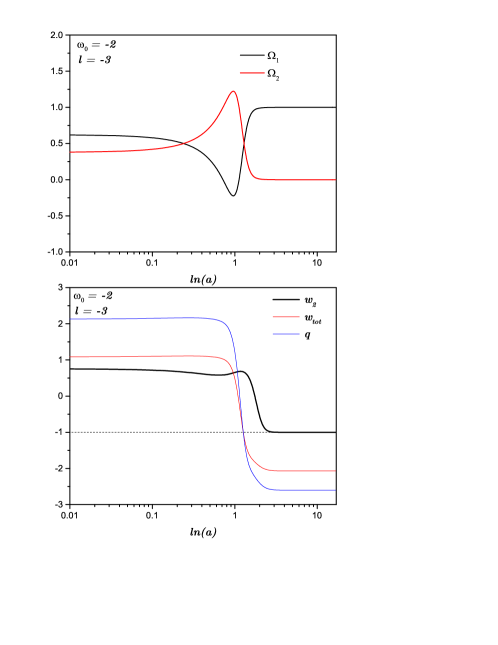
Figure 4: Qualitative evolution of the dimensionless energy densities $\Omega_{1},\Omega_{2}$ and the observables $w_{2},{w_{\text{tot}}},q$ vs $\ln(a)$ for $W(\psi)=W_{0}e^{k\psi}$ and $V(\varphi)=V_{0}e^{l\varphi}$ with $\omega_{0}=-2,l=-3$.

In the Fig. 4 is presented evolution of the dimensionless energy densities $\Omega_{1},\Omega_{2}$ and the observables $w_{2},{w_{\text{tot}}},q$ vs $\ln(a)$ for $W(\psi)=W_{0}e^{k\psi}$ and $V(\varphi)=V_{0}e^{l\varphi}$ with $\omega_{0}=-2,l=-3$.

5.2 Case: $W(\psi)=W_{0}\psi^{2\beta}$ and $V(\varphi)=V_{0}e^{(\beta-1)\varphi}$

For this model we have the same results for the first nine equilibrium points in Table 2, in section 5.1 replacing $l=\beta-1,k=2\beta$, and the additional equilibrium points $P_{11}-P_{15}$.

The relevant early- and late-time attractors are the following:

• The stable manifold of $P_{1}$ is three dimensional for $\beta>2,\omega_{0}\geq\frac{1}{6}(16\beta-41)$.

• The equilibrium point $P_{5}$ is a sink for $\beta>0,\omega_{0}<-\frac{3}{2}$.

• The equilibrium point $P_{6}$ is a sink for $\beta<0,\omega_{0}<-\frac{3}{2}$.

• The equilibrium point $P_{6}$ is a sink for $-1<\beta\leq 0,\frac{1}{6}(\beta-5)(\beta+1)<\omega_{0}<0$, or $\beta>0,-\frac{5}{6}<\omega_{0}<0$. It is a source for $\beta\leq-1,\omega_{0}>\frac{1}{6}(\beta-5)(\beta+1)$, or $\beta>-1,\omega_{0}>0$.

• $P_{13}$ is a source for $\omega_{0}\in\mathbb{R},\beta=0$, or $0<\beta<3,\omega_{0}<-\frac{3}{2}$.

• The observables for $P_{11,12}$ and $P_{14,15}$ have to be evaluated for specific choices of the parameters.

6 Some results for arbitrary potentials

In the sections 4.1 and 4.2, we have investigated an exponential potential $V(\varphi)$ for which $s$ is a constant such that $h$ is only a function of $\lambda$ that depends on the choice of $W$, and $F$ is identically zero. For complementing these results, in this section we comment about the generic features of the equilibrium points of (31) for arbitrary $h(\lambda,s)$ and $F(s)$ functions.

Since the system is form-invariant under the change
$(y,z,\lambda)\rightarrow(-y,-z,-\lambda)$. Thus, without losing generality we can investigate just the sector $y\geq 0,z\geq 0,\lambda\geq 0$. Henceforth, we will focus on the stability properties of the system (31) for the state vector $(x,y,z,\lambda)$ defined in the phase space

$$\Big{\{}(x,y,z,s,\lambda)\in\mathbb{R}^{5}:-\sqrt{6}x+x^{2}\omega_{0}+y^{2}+z^{2}\leq 1,y\geq 0,z\geq 0,\lambda\geq 0,s\in\mathbb{R}\Big{\}}.$$ (61)

The equilibrium points of (31) that are independent of $h(s,\lambda)$ are summarized below. In table 3 are shown the cosmological parameters corresponding to the formulation in the dilatonic frame as given by Eqs. (9) for the equilibrium points in the invariant set $\lambda=0$ for arbitrary potentials.

1. $(x,y,z,\lambda,s)=\left(0,\frac{\sqrt{2}}{\sqrt{1-s_{c}}},0,0,s_{c}\right)$.
   Exists for $s_{c}\leq-1$.
   The eigenvalues are
   $\Big{\{}0,0,-3$,
   $\frac{1}{2}\left(-\frac{\sqrt{3}\sqrt{\left(s_{c}-1\right)\left(16F\left(s_{c}\right)+\left(s_{c}-1\right)\left(16s_{c}+6\omega_{0}+25\right)\right)}}{\sqrt{2\omega_{0}+3}\left(s_{c}-1\right)}-3\right)$,
   $\frac{1}{2}\left(\frac{\sqrt{3}\sqrt{\left(s_{c}-1\right)\left(16F\left(s_{c}\right)+\left(s_{c}-1\right)\left(16s_{c}+6\omega_{0}+25\right)\right)}}{\sqrt{2\omega_{0}+3}\left(s_{c}-1\right)}-3\right)\Big{\}}$.
   This line of equilibrium points contains the cases $s_{c}=\hat{s}:F(\hat{s})=0$, for which the eigenvalues simplifies to
   $\left\{0,0,-3,\frac{1}{2}\left(-\frac{\sqrt{16\hat{s}+6\omega_{0}+25}}{\sqrt{2\omega_{0}+3}}-3\right),\frac{1}{2}\left(\frac{\sqrt{16\hat{s}+6\omega_{0}+25}}{\sqrt{2\omega_{0}+3}}-3\right)\right\}$.
   It is non-hyperbolic. The stable manifold of $P_{1}$ is three dimensional provided
   $s_{c}\leq-1,1-s_{c}^{2}<F\left(s_{c}\right)\leq-\frac{1}{16}\left(s_{c}-1\right)\left(16s_{c}+6\omega_{0}+25\right)$, in other case the stable manifold is a lower dimensional.

2. $(x,y,z,\lambda,s)=\left(-\sqrt{\frac{2}{3}},0,\sqrt{-\frac{2\omega_{0}}{3}-1},0,\hat{s}\right)$, where $F(\hat{s})=0$.
   Exists for $\omega_{0}<-\frac{3}{2}$.
   The eigenvalues are $\left\{6,-1,1,\hat{s}+2,2F^{\prime}\left(\hat{s}\right)\right\}$.
   The equilibrium point is a saddle and has a four dimensional unstable manifold provided $\hat{s}>-2,F^{\prime}(\hat{s})>0$. In other case, the unstable manifold is a lower dimensional.

3. $(x,y,z,\lambda,s)=\left(\frac{\sqrt{6}}{\hat{s}-1},\frac{\sqrt{\hat{s}+2}}{\hat{s}-1},\frac{\sqrt{\hat{s}\left(\hat{s}+3\right)-6\omega_{0}-7}}{\hat{s}-1},0,\hat{s}\right)$.
   Exists for

   1. $\hat{s}>1,\omega_{0}<-\frac{3}{2}$, or

   2. $\hat{s}>1,-\frac{3}{2}<\omega_{0}\leq\frac{1}{6}\left(\hat{s}^{2}+3\hat{s}-7\right)$.

   The eigenvalues are
   $\Big{\{}\frac{3}{\hat{s}-1},6,-\frac{3}{2\left(\hat{s}-1\right)}-\frac{\sqrt{-8\hat{s}\left(\hat{s}\left(\hat{s}+5\right)-6\omega_{0}-1\right)+102\omega_{0}+121}}{2\left(\hat{s}-1\right)\sqrt{\frac{2\omega_{0}}{3}+1}}$,
   $-\frac{3}{2\left(\hat{s}-1\right)}+\frac{\sqrt{-8\hat{s}\left(\hat{s}\left(\hat{s}+5\right)-6\omega_{0}-1\right)+102\omega_{0}+121}}{2\left(\hat{s}-1\right)\sqrt{\frac{2\omega_{0}}{3}+1}},-\frac{6F^{\prime}\left(\hat{s}\right)}{\hat{s}-1}\Big{\}}$.
   It is a saddle.

4. $(x,y,z,\lambda,s)=\left(\frac{\sqrt{6}}{\hat{s}-1},\frac{\sqrt{\hat{s}+2}}{1-\hat{s}},\frac{\sqrt{\hat{s}\left(\hat{s}+3\right)-6\omega_{0}-7}}{1-\hat{s}},0,\hat{s}\right)$. Exists for

   1. $\hat{s}=-2,\omega_{0}<-\frac{3}{2}$, or

   2. $-2<\hat{s}<-1,\omega_{0}\leq\frac{1}{6}\left(\hat{s}^{2}+3\hat{s}-7\right)$, or

   3. $-1<\hat{s}<1,-\frac{3}{2}<\omega_{0}\leq\frac{1}{6}\left(\hat{s}^{2}+3\hat{s}-7\right)$, or

   4. $-1\leq\hat{s}<1,\omega_{0}<-\frac{3}{2}$.

   The eigenvalues are
   $\Big{\{}\frac{3}{\hat{s}-1},6,-\frac{3}{2\left(\hat{s}-1\right)}-\frac{\sqrt{-8\hat{s}\left(\hat{s}\left(\hat{s}+5\right)-6\omega_{0}-1\right)+102\omega_{0}+121}}{2\left(\hat{s}-1\right)\sqrt{\frac{2\omega_{0}}{3}+1}}$,
   $-\frac{3}{2\left(\hat{s}-1\right)}+\frac{\sqrt{-8\hat{s}\left(\hat{s}\left(\hat{s}+5\right)-6\omega_{0}-1\right)+102\omega_{0}+121}}{2\left(\hat{s}-1\right)\sqrt{\frac{2\omega_{0}}{3}+1}},-\frac{6F^{\prime}\left(\hat{s}\right)}{\hat{s}-1}\Big{\}}$.
   It is a saddle.

5. $(x,y,z,\lambda,s)=\left(\frac{2\sqrt{\frac{2}{3}}}{2\omega_{0}+1},0,0,0,\hat{s}\right)$, where $F(\hat{s})=0$.
   Exists for

   1. $\omega_{0}<-\frac{3}{2}$, or

   2. $-\frac{5}{6}\leq\omega_{0}<-\frac{1}{2}$, or

   3. $\omega_{0}>-\frac{1}{2}$.

   The eigenvalues are
   $\left\{\frac{2}{2\omega_{0}+1},-\frac{2\left(\hat{s}-1\right)}{2\omega_{0}+1},-3,-\frac{6\omega_{0}+5}{2\omega_{0}+1},-\frac{4F^{\prime}\left(\hat{s}\right)}{2\omega_{0}+1}\right\}$.
   It is a sink for $\omega_{0}<-\frac{3}{2},\hat{s}<1,F^{\prime}\left(\hat{s}\right)<0$. It is a saddle otherwise.

6. $(x,y,z,\lambda,s)$
   $=\left(-\frac{\sqrt{\frac{2}{3}}\left(\hat{s}+1\right)}{\hat{s}-2\left(\omega_{0}+1\right)},\frac{\sqrt{\left(2\omega_{0}+3\right)\left(-\hat{s}\left(\hat{s}+2\right)+6\omega_{0}+8\right)}}{\sqrt{3}\left(\hat{s}-2\left(\omega_{0}+1\right)\right)},0,0,\hat{s}\right)$, where $F(\hat{s})=0$. Exists for

   1. $\hat{s}<-1,\omega_{0}=\frac{1}{6}\left(\hat{s}-2\right)\left(\hat{s}+4\right)$, or

   2. $\hat{s}<-1,\omega_{0}<\frac{1}{2}\left(\hat{s}-2\right)$, or

   3. $-1\leq\hat{s}\leq 2,\omega_{0}<-\frac{3}{2}$, or

   4. $-1<\hat{s}<2,\frac{1}{6}\left(\hat{s}-2\right)\left(\hat{s}+4\right)\leq\omega_{0}<\frac{1}{2}\left(\hat{s}-2\right)$, or

   5. $\hat{s}>2,\omega_{0}=\frac{1}{6}\left(\hat{s}-2\right)\left(\hat{s}+4\right)$, or

   6. $\hat{s}>2,\omega_{0}<-\frac{3}{2}$.

   The eigenvalues are
   $\Big{\{}-\frac{\hat{s}+1}{\hat{s}-2\omega_{0}-2},-\frac{2\left(\hat{s}-1\right)\left(\hat{s}+1\right)}{\hat{s}-2\omega_{0}-2},-\frac{\hat{s}^{2}+2\hat{s}-6\omega_{0}-8}{\hat{s}-2\omega_{0}-2},-\frac{\hat{s}^{2}+3\hat{s}-6\omega_{0}-7}{\hat{s}-2\omega_{0}-2},\frac{2\left(\hat{s}+1\right)F^{\prime}\left(\hat{s}\right)}{\hat{s}-2\omega_{0}-2}\Big{\}}$.
   It is a sink for $\omega_{0}<-\frac{3}{2},\hat{s}>1,F^{\prime}\left(\hat{s}\right)<0$, or a saddle otherwise.

7. $(x,y,z,\lambda,s)$
   $=\left(-\frac{\sqrt{\frac{2}{3}}\left(\hat{s}+1\right)}{\hat{s}-2\left(\omega_{0}+1\right)},-\frac{\sqrt{\left(2\omega_{0}+3\right)\left(-\hat{s}\left(\hat{s}+2\right)+6\omega_{0}+8\right)}}{\sqrt{3}\left(\hat{s}-2\left(\omega_{0}+1\right)\right)},0,0,\hat{s}\right)$,
   where $F(\hat{s})=0$.
   Exists for

   1. $\hat{s}<-1,\frac{1}{2}\left(\hat{s}-2\right)<\omega_{0}<-\frac{3}{2}$, or

   2. $\hat{s}<-1,\omega_{0}\geq\frac{1}{6}\left(\hat{s}-2\right)\left(\hat{s}+4\right)$, or

   3. $\hat{s}=-1,\omega_{0}>-\frac{3}{2}$, or

   4. $-1<\hat{s}<2,\omega_{0}=\frac{1}{6}\left(\hat{s}-2\right)\left(\hat{s}+4\right)$, or

   5. $-1<\hat{s}<2,\omega_{0}>\frac{1}{2}\left(\hat{s}-2\right)$, or

   6. $\hat{s}=2,\omega_{0}>0$, or

   7. $\hat{s}>2,\omega_{0}\geq\frac{1}{6}\left(\hat{s}-2\right)\left(\hat{s}+4\right)$.

   The eigenvalues are
   $\Big{\{}-\frac{\hat{s}+1}{\hat{s}-2\omega_{0}-2},-\frac{2\left(\hat{s}-1\right)\left(\hat{s}+1\right)}{\hat{s}-2\omega_{0}-2},-\frac{\hat{s}^{2}+2\hat{s}-6\omega_{0}-8}{\hat{s}-2\omega_{0}-2}$,
   $-\frac{\hat{s}^{2}+3\hat{s}-6\omega_{0}-7}{\hat{s}-2\omega_{0}-2},\frac{2\left(\hat{s}+1\right)F^{\prime}\left(\hat{s}\right)}{\hat{s}-2\omega_{0}-2}\Big{\}}$.
   It is always a saddle point.

8. $(x,y,z,\lambda,s)=\left(\frac{\sqrt{3}-\sqrt{2\omega_{0}+3}}{\sqrt{2}\omega_{0}},0,0,0,\hat{s}\right)$, where $F(\hat{s})=0$.
   Exists for $\omega_{0}>-\frac{3}{2},\omega_{0}\neq 0$.
   The eigenvalues are
   $\Big{\{}-\frac{\sqrt{6\omega_{0}+9}-3}{2\omega_{0}},-\frac{\sqrt{6\omega_{0}+9}-3}{2\omega_{0}},\frac{6\omega_{0}-\sqrt{6\omega_{0}+9}+3}{\omega_{0}}$,
   $\frac{\hat{s}\left(\sqrt{6\omega_{0}+9}-3\right)+6\omega_{0}-2\sqrt{6\omega_{0}+9}+6}{2\omega_{0}},\frac{\left(\sqrt{6\omega_{0}+9}-3\right)F^{\prime}\left(\hat{s}\right)}{\omega_{0}}\Big{\}}$.
   It is a saddle.

9. $(x,y,z,\lambda,s)=\left(\frac{\sqrt{3}+\sqrt{2\omega_{0}+3}}{\sqrt{2}\omega_{0}},0,0,0,\hat{s}\right)$, where $F(\hat{s})=0$.
   Exists for $\omega_{0}>-\frac{3}{2},\omega_{0}\neq 0$.
   The eigenvalues are
   $\Big{\{}\frac{\sqrt{6\omega_{0}+9}+3}{2\omega_{0}},\frac{\sqrt{6\omega_{0}+9}+3}{2\omega_{0}},\frac{6\omega_{0}+\sqrt{6\omega_{0}+9}+3}{\omega_{0}}$,
   $\frac{-\hat{s}\left(\sqrt{6\omega_{0}+9}+3\right)+6\omega_{0}+2\sqrt{6\omega_{0}+9}+6}{2\omega_{0}},-\frac{\left(\sqrt{6\omega_{0}+9}+3\right)F^{\prime}\left(\hat{s}\right)}{\omega_{0}}\Big{\}}$.
   It is a source for

   1. $\hat{s}\leq 2,\omega_{0}>0,F^{\prime}\left(\hat{s}\right)<0$, or

   2. $\hat{s}>2,\omega_{0}>\frac{1}{6}\left(\hat{s}-2\right)\left(\hat{s}+4\right),F^{\prime}\left(\hat{s}\right)<0$.

   It is a sink for

   1. $\hat{s}\leq 1,-\frac{5}{6}<\omega_{0}<0,F^{\prime}\left(\hat{s}\right)<0$, or

   2. $1<\hat{s}<2,\frac{1}{6}\left(\hat{s}-2\right)\left(\hat{s}+4\right)<\omega_{0}<0,F^{\prime}\left(\hat{s}\right)<0$.

As we see, the stability of these points depends on the character of the zeros $\hat{s}$ of the function $F(s)$, and their first order derivative evaluated at $\hat{s}$. The function $F(s)$ for the most common quintessence potentials Escobar:2013js is displayed in table 1.

The points $P_{1}$- $P_{9}$ were found in the previous three examples, for which $s$ is a constant, such that $h$ is only a function of $\lambda$ that depends on the choice of $W$, and $F$ is identically zero ( the problem can be reduced in one dimension). When $F(s)$ is not trivial, the above classification can be implemented straightforwardly, as for the specific choices of $F$ in table 1. The search of the equilibrium points with $\lambda\neq 0$ is not an easy task, and the success on it depends crucially on the choice of $h(s,\lambda)$. Indeed, for a given $h$, there are equilibrium points on the surface $x-2\lambda z(h(s,\lambda)-1)=0$. On this surface the existence conditions of an equilibrium point are $\Big{\{}(x,y,z,\lambda,s)\in\mathbb{R}^{5}:y\geq 0,z\geq 0,\lambda\geq 0,2\omega_{0}+3\neq 0,\\ z^{2}\left(4\lambda^{2}\omega_{0}(h(s,\lambda)-1)^{2}+1\right)+y^{2}\leq 2\sqrt{6}\lambda z(h(s,\lambda)-1)+1\Big{\}}.$

For example, the given $h(s,\lambda)\equiv 1$, we have the additional equilibrium points $(x,y,z,\lambda,s)=\left(0,0,\sqrt{\frac{2}{3}},2,s_{c}\right)$, where $h(s_{c},2)=1$. For $h(s,\lambda)=1-\frac{1}{2\beta}$, we have the additional points $P_{11}$- $P_{15}$ investigated in section 4.2.

Table 3: Cosmological parameters corresponding to the formulation in the dilatonic frame as given by Eqs. (9) for the equilibrium points in the invariant set $\lambda=0$ for arbitrary potentials.

Equil.	$\Omega_{2}$	$w_{1}$	$w_{2}$	${w_{\text{tot}}}$
Points
$P_{1}$	$\frac{s_{c}+1}{s_{c}-1}$	$-1$	$-1$	$-1$
$P_{2}(\hat{s})$	$-\frac{2\omega_{0}}{3}-1$	$1$	$1$	$1$
$P_{3}(\hat{s})$	$\frac{\hat{s}\left(\hat{s}+3\right)-6\omega_{0}-7}{\left(\hat{s}-1\right)^{2}}$	$1$	$1$	$1$
$P_{4}(\hat{s})$	$\frac{\hat{s}\left(\hat{s}+3\right)-6\omega_{0}-7}{\left(\hat{s}-1\right)^{2}}$	$1$	$1$	$1$
$P_{5}(\hat{s})$	$\frac{\left(2\omega_{0}+3\right)\left(6\omega_{0}+5\right)}{3\left(2\omega_{0}+1\right){}^{2}}$	$-1$	$-1$	$-1$
$P_{6}(\hat{s})$	$0$	$-\frac{2\left(\hat{s}^{2}-1\right)}{3\left(\hat{s}-2\left(\omega_{0}+1\right)\right)}-1$	Indeterminate	$-\frac{2\left(\hat{s}^{2}-1\right)}{3\left(\hat{s}-2\left(\omega_{0}+1\right)\right)}-1$
$P_{7}(\hat{s})$	$0$	$-\frac{2\left(\hat{s}^{2}-1\right)}{3\left(\hat{s}-2\left(\omega_{0}+1\right)\right)}-1$	Indeterminate	$-\frac{2\left(\hat{s}^{2}-1\right)}{3\left(\hat{s}-2\left(\omega_{0}+1\right)\right)}-1$
$P_{8}(\hat{s})$	$0$	$\frac{3\omega_{0}-\sqrt{6\omega_{0}+9}+3}{3\omega_{0}}$	$-1$	$\frac{3\omega_{0}-\sqrt{6\omega_{0}+9}+3}{3\omega_{0}}$
$P_{9}(\hat{s})$	$0$	$\frac{3\omega_{0}+\sqrt{6\omega_{0}+9}+3}{3\omega_{0}}$	$-1$	$\frac{3\omega_{0}+\sqrt{6\omega_{0}+9}+3}{3\omega_{0}}$

7 Discussion and Conclusions

In this work the Brans-Dicke action has been considered in the cosmological scenario of FLRW spacetime with spatially flat curvature; while a minimally coupled scalar field was considered as a matter source. We show that this action in the Einstein frame provides the dilatonic action integral and it is equivalent to the $\sigma$-models. The method of the group invariant transformations, i.e., symmetries of differential equations was applied in order to constraint the free functions of the theory, and determine conservation laws for the gravitational field equations. We found that for a family of potentials there exists a Noetherian conservation law. From the admitted symmetries we derived the zero-order invariants and we derived specific solutions for the field equations which correspond to matter-like dominant eras. Additionally, we have studied the stability of the equilibrium points of the dynamical system for specific and arbitrary potentials.

For the model 1, corresponding to the formulation in the dilatonic frame as given by Eqs. (9) for $W(\psi)=W_{0}e^{k\psi}$ and $V(\varphi)=V_{0}e^{l\varphi}$, we have obtained the following main results. The equilibrium for $P_{1}$ corresponds to a solution with $w_{\text{tot}}=-1$. We have proved that its center manifold is stable for $1<l\leq\frac{1}{16}\left(6\omega_{0}+25\right)$. We show this solution is an attractor in the dilatonic frame but it is an intermediate accelerated solution $a\simeq e^{At^{p}},p:=\frac{2}{2+l},\quad\frac{32}{57+6\omega_{0}}<p<\frac{2}{3},\;\text{as}\;t\rightarrow\infty$, and not a de Sitter solution. The exponent $p$ is reduced, in a particular case, to the exponent already found for the Jordan’s and Einstein’s frames by Cid:2015pja . We have obtained some equilibrium points, $P_{2},P_{3}$ and $P_{4}$, that represent stiff solutions which are saddle. The equilibrium point $P_{5}$, satisfies $w_{\text{tot}}=-1$. It is a sink for $l>-1,\omega_{0}<-\frac{3}{2}$ or a saddle otherwise. The equilibrium point $P_{6}$, corresponds to a solution where the energy density of the dilatonic field is dominant and the energy density of the quintessence field is negligible. According to whether ${w_{\text{tot}}}:=\frac{2\left(l^{2}-1\right)}{3\left(l+2\omega_{0}+2\right)}-1$ satisfies ${w_{\text{tot}}}<-1,{w_{\text{tot}}}=-1$ or $-1<{w_{\text{tot}}}<-\frac{1}{3}$ we have found it represents a phantom solution, a solution with $w_{\text{tot}}=-1$ or a quintessence solution. It is a sink for $l<-1,\omega_{0}<-\frac{3}{2}$. It is a saddle otherwise. Other equilibrium point as $P_{8}$ mimics a standard dark matter source with $0<w_{\text{tot}}<1$. It is a saddle. The equilibrium point $P_{9}$ corresponds to a solution where the energy density of the dilatonic field is dominant and the energy density of the quintessence field is negligible. Furthermore, $w_{1}=\frac{3\omega_{0}+\sqrt{6\omega_{0}+9}+3}{3\omega_{0}}$, $w_{2}=-1$, and $w_{\text{tot}}=\frac{3\omega_{0}+\sqrt{6\omega_{0}+9}+3}{3\omega_{0}}$. That is, the second fluid behaves as a cosmological constant whereas the effective equation of state (of the total cosmic budget) is that of quintessence field for $-\frac{9}{8}<\omega_{0}<-\frac{5}{6}$, a cosmological constant for $\omega_{0}=-\frac{5}{6}$ and the phantom field for $-\frac{5}{6}<\omega_{0}<0$. It is a sink for $-2<l\leq-1,\frac{1}{6}(l-4)(l+2)<\omega_{0}<0$, or $l>-1,-\frac{5}{6}<\omega_{0}<0$ (in both cases is a phantom attractor). It is a source for $l\leq-2,\omega_{0}>\frac{1}{6}(l-4)(l+2)$, or $l>-2,\omega_{0}>0$ (and it behaves as a standard matter source then). It is a saddle otherwise. Finally, the equilibrium point $P_{10}$ is dominated by the quintessence field and the contribution of the dilatonic field to the total energy density is negligible. It satisfies $w_{2}=\frac{1}{3}$ and ${w_{\text{tot}}}=\frac{1}{3}$. This means that the corresponding cosmological solution mimics radiation. Interestingly, it is a saddle with a three dimensional stable manifold provided $\omega_{0}\geq\frac{45}{2}$. These results illustrate the capabilities of the model.

For the second model, we have $V\left(\varphi\right)=V_{0}e^{\left(\beta-1\right)\varphi}~{}\ ,~{}W\left(\psi\right)=W_{0}\psi^{2\beta}$. The particular parameters where chosen to lead to Noether pointlike symmetries. For this model, we have the same results for the first nine equilibrium points in Table 2 , in section 5.1, and discussed before, by replacing $l=\beta-1,k=2\beta$. We have found the additional equilibrium points $P_{11}-P_{15}$, whose stability and cosmological observables have to be evaluated numerically.

We recall that the points $P_{1}$- $P_{9}$ were found in the previous examples, under the assumption $s$ is a constant such that $h$ is only a function of $\lambda$ that depends on the choice of $W$, and $F$ is identically zero (that is, the problem can be reduced in one dimension). When $F(s)$ is not trivial, the above classification can be implemented straightforwardly, as for the specific choices of $F$ in table 1. The search of the equilibrium points with $\lambda\neq 0$ is not an easy task, and the success on it depends crucially on the choice of $h(s,\lambda)$. For example, given $h(s,\lambda)\equiv 1$, we have the additional equilibrium points $(x,y,z,\lambda,s)=\left(0,0,\sqrt{\frac{2}{3}},2,s_{c}\right)$, where $h(s_{c},2)=1$. For $h(s,\lambda)=1-\frac{1}{2\beta}$, we have the additional points $P_{11}$- $P_{15}$ investigated in section 4.2. A more complete study requires the specification of the free functions and this is far the scope of the present research.

A possible generalization on the context of scalar-tensor theories will be interesting. In this respect, after dealing with two simple examples, we made the first steps to provide a complete dynamical system analysis of dilatonic JBD cosmology keeping the potentials arbitrary, which is a major improvement since it allows for the extraction of information that is related to the foundations of the cosmological model and not to the specific potentials forms. In particular, we apply an extended version of the method of $f$-devisers Escobar:2013js ; Fadragas:2013ina ; delCampo:2013vka - in the sense that it was developed for two free functions such that additionally to the $f$-deviser we have an $h$-deviser. Using this approach, one first performs the analysis without the need of a priori specification of the potentials forms. At the end, one just substitutes the specific potential forms in the results, instead of having to repeat the whole dynamical elaboration from the start. Therefore, the results are richer and more general, revealing the full capabilities of dilatonic JBD cosmology.

References

(1) M. Tegmark et al., Astrophys. J. 606, 702 (2004)
(2) M. Kowalski et al., Astrophys. J. 686, 749 (2008)
(3) E. Komatsu et al., Astrophys. J. Suppl. Ser. 180,
330 (2009).
(4) N. Suzuki et. al., Astrophys. J. 746, 85 (2012)
(49)
R. V. Wagoner,
Phys. Rev. D 1 (1970), 3209-3216
(50)
J. O’ Hanlon,
J. Phys. A 5 (1972), 803-811
(51)
J. O’ Hanlon and B. Tupper,
Nuovo Cim. B 7 (1972), 305-312
(52)
J. Bekenstein,
Phys. Rev. D 15 (1977), 1458-1468
(53)
P. G. Bergmann,
Int. J. Theor. Phys. 1 (1968), 25-36
(54)
K. Nordtvedt, Jr.,
Astrophys. J. 161 (1970), 1059-1067
(55)
M. B. Green, C. M. Hull and P. K. Townsend,
Phys. Lett. B 382 (1996), 65-72
(56)
A. Abramovici, W. E. Althouse, R. W. Drever, Y. Gursel, S. Kawamura, F. J. Raab, D. Shoemaker, L. Sievers, R. E. Spero, K. S. Thorne, R. E. Vogt, R. Weiss, S. E. Whitcomb and M. E. Zucker,
Science 256 (1992), 325-333
(57)
A. Serna, J. Alimi and A. Navarro,
Class. Quant. Grav. 19 (2002), 857-874
(58)
A. Serna and J. Alimi,
Phys. Rev. D 53 (1996), 3087-3098
(59)
J. D. Barrow and P. Parsons,
Phys. Rev. D 55 (1997), 1906-1936
(60)
C. Will,
“Theory and experiment in gravitational physics,”
(61)
C. M. Will,
Living Rev. Rel. 9, 3 (2006)
(62)
J. D. Barrow and K. i. Maeda,
Nucl. Phys. B 341 (1990), 294-308
(63)
V. Faraoni and M. N. Jensen,
Class. Quant. Grav. 23 (2006), 3005-3016
(64)
A. R. Liddle and D. Wands,
Phys. Rev. D 45 (1992), 2665-2673
(65)
D. La and P. J. Steinhardt,
Phys. Rev. Lett. 62 (1989), 376
(66)
C. Mathiazhagan and V. Johri,
Class. Quant. Grav. 1 (1984), L29-L32
(67)
S. J. Kolitch,
Annals Phys. 246 (1996), 121-132
(68)
C. Romero and A. Barros,
Gen. Rel. Grav. 25 (1993), 491-502
(69)
N. Kaloper and K. A. Olive,
Phys. Rev. D 57, 811-822 (1998)
(70)
G. Magnano, M. Ferraris and M. Francaviglia,
Class. Quant. Grav. 7 (1990), 557-570
(71)
S. Cotsakis,
Phys. Rev. D 47 (1993), 1437-1439
(72)
P. Teyssandier,
Phys. Rev. D 52, 6195-6197 (1995)
(73)
H. Schmidt,
Phys. Rev. D 52, 6198 (1995)
(74)
S. Cotsakis,
Phys. Rev. D 52, 6199-6200 (1995)
(75)
S. Capozziello, R. de Ritis and A. A. Marino,
Class. Quant. Grav. 14, 3243-3258 (1997)
(76)
G. Magnano and L. M. Sokolowski,
Phys. Rev. D 50, 5039-5059 (1994)
(77)
V. Faraoni, E. Gunzig and P. Nardone,
Fund. Cosmic Phys. 20, 121 (1999)
(78)
V. Faraoni,
Phys. Rev. D 75, 067302 (2007)
(79)
V. Faraoni and S. Nadeau,
Phys. Rev. D 75, 023501 (2007)
(80) A. A. Coley. Dynamical systems and cosmology,
Dordrecht, Netherlands: Kluwer (2003).
(81) T. Gonzalez, G. Leon and I. Quiros, Class. Quant. Grav. 23,3165 (2006).
(82)
J. P. Mimoso and D. Wands,
Phys. Rev. D 51 (1995), 477-489
(83)
J. P. Mimoso and D. Wands,
Phys. Rev. D 52 (1995), 5612-5627
(84)
A. Coley,
Gen. Rel. Grav. 31 (1999), 1295
(85) T.P. Sotiriou and V. Faraoni, Rev. Mod. Phys.
82, 451-497 (2010).
(86) A. Y. Kamenshchik, E. O. Pozdeeva,
A. Tronconi, G. Venturi and S. Y. Vernov,
Class. Quant. Grav. 31, 105003 (2014).
(87) A. Y. Kamenshchik, E. O. Pozdeeva,
A. Tronconi, G. Venturi and S. Y. Vernov,
Class. Quant. Grav. 33, no. 1, 015004 (2016).
(88) A. Y. Kamenshchik, E. O. Pozdeeva,
A. A. Starobinsky, A. Tronconi, G. Venturi and S. Y. Vernov,
Phys. Rev. D 97, no. 2, 023536 (2018).
(89) M. Tsamparlis, A. Paliathanasis, S. Basilakos and S.
Capozziello, Gen. Rel. Gravit. 45, 2003 (2013).
(90) A. Paliathanasis and M. Tsamparlis, Phys. Rev. D 90, 043529 (2014).
(91) A. Paliathanasis, M. Tsamparlis, S. Basilakos and J.D.
Barrow, Phys. Rev. D 93, 043528 (2016).
(92) A. Zampeli, T. Pailas, P.A. Terzis and T. Christodoulakis,
JCAP 1605, 066 (2015).
(93) A. Paliathanasis, Gen. Rel. Gravit. 51, 101 (2019)
(94) A. Cid, G. Leon and Y. Leyva,
JCAP 1602, no. 02, 027 (2016).
(95) S. Bahamonte, C.G. Boehmer, S. Carloni, E.J. Copeland, W. Fang and N. Tamanini, Phys. Rept. 775-777, 1 (2018)
(96)
I. Quiros,
Int. J. Mod. Phys. D 28 (2019) no.07, 1930012
doi:10.1142/S021827181930012X
[arXiv:1901.08690 [gr-qc]].
(97) E. J. Copeland, S. Mizuno and M. Shaeri,
Phys. Rev. D 79, 103515 (2009).
(98) D. Escobar, C. R. Fadragas, G. Leon and Y. Leyva,
Class. Quant. Grav. 29, 175005 (2012).
(99) D. Escobar, C. R. Fadragas, G. Leon and Y. Leyva,
Class. Quant. Grav. 29, 175006 (2012).
(100) A. B. Burd and J. D. Barrow,
Nucl. Phys. B 308, 929 (1988).
(101) R. Tavakol, Introduction to dynamical systems, in
Dynamical systems in cosmology, J. Wainwright and G. F. R. Ellis
(eds) Cambridge University Press, Cambridge, England (1997).
(102) E. J. Copeland, A. R. Liddle and D. Wands,
Phys. Rev. D 57, 4686 (1998).
(103) Y. Gong, A. Wang and Y. Z. Zhang,
Phys. Lett. B 636, 286 (2006).
(104) M. R. Setare and E. N. Saridakis,
Phys. Rev. D 79, 043005 (2009).
(105) X. -m. Chen, Y. -g. Gong and E. N. Saridakis,
JCAP 0904, 001 (2009).
(106) G. Gupta, E. N. Saridakis and A. A. Sen,
Phys. Rev. D 79, 123013 (2009).
(107) H. Farajollahi, A. Salehi, F. Tayebi and
A. Ravanpak,
JCAP 1105, 017 (2011).
(108) C. Xu, E. N. Saridakis and G. Leon,
JCAP 1207, 005 (2012).
(109) G. Leon, J. Saavedra and E. N. Saridakis,
Class. Quant. Grav. 30, 135001 (2013).
(110) T. Matos, J. -R. Luevano, I. Quiros,
L. A. Urena-Lopez, J. A. Vazquez,
Phys. Rev. D80, 123521 (2009).
(111) Y. Leyva, D. Gonzalez, T. Gonzalez, T. Matos,
I. Quiros,
Phys. Rev. D80, 044026 (2009).
(112) L. A. Urena-Lopez, JCAP 1203, 035 (2012).
(113) A. D. Rendall,
Class. Quant. Grav. 21, 2445-2454 (2004).
(114) W. Fang, Y. Li, K. Zhang, H. -Q. Lu,
Class. Quant. Grav. 26, 155005 (2009).
(115) G. Leon,
Class. Quant. Grav. 26, 035008 (2009).
(116) D. Escobar, C. R. Fadragas, G. Leon and Y. Leyva,
Astrophys. Space Sci. 349, 575 (2014).
(117) S. del Campo, C. R. Fadragas, R. Herrera,
C. Leiva, G. Leon and J. Saavedra, Phys. Rev. D 88, 023532 (2013).
(118) C. R. Fadragas, G. Leon and E. N. Saridakis,
Class. Quant. Grav. 31, 075018 (2014).
(119) P.A.M. Dirac, Can. J. Math. 2, 129 (1950).
(120) S.V. Chervon, Quantum Matter 2, 71 (2013).
(121) V.B. Bezerra, S. Chervon and C. Romero, Int. J. Mod. Phys. D 14, 1927 (2005).
(122) N. Dimakis, A. Karagiorgos, A. Zampeli, A. Paliathanasis, T.
Christodoulakis and P.A. Terzis, Phys. Rev. D. 93, 123518.
(123) J. Yearsley and J. D. Barrow, Class. Quant. Grav. 13, 2693 (1996).
(124) S. A. Pavluchenko, Phys. Rev. D 67,103518 (2003).
(125) R. Cardenas, T. Gonzalez, Y. Leiva, O. Martin and
I. Quiros, Phys. Rev. D 67, 083501 (2003).
(126) T. Barreiro, E. J. Copeland and N. J. Nunes,
Phys. Rev. D 61, 127301 (2000).
(127) T. Gonzalez, R. Cardenas, I. Quiros and Y. Leyva,
Astrophys. Space Sci. 310, 13 (2007).
(128) V. Sahni and L. -M. Wang, Phys. Rev. D 62, 103517 (2000).
(129) V. Sahni and A. A. Starobinsky, Int. J. Mod. Phys. D 9, 373 (2000).
(130) J. E. Lidsey, T. Matos and L. A. Urena-Lopez,
Phys. Rev. D 66, 023514, (2002).
(131) T. Matos and L. A. Urena-Lopez, Class. Quant. Grav. 17, L75 (2000).
(132) B. Ratra and P. J. E. Peebles,
Phys. Rev. D 37, 3406 (1988).
(133) C. Wetterich,
Nucl. Phys. B 302, 668 (1988).
(134) L. A. Urena-Lopez and T. Matos, Phys. Rev. D 62, 081302 (2000).
(135) G. Leon and E. N. Saridakis,
Class. Quant. Grav. 28, 065008 (2011).
(136) R. García-Salcedo, T. González and
I. Quiros,
Phys. Rev. D 92, no. 12, 124056 (2015).