FDTD simulation algorithm of magnetized plasma media
Aleksandr Friman
Solid State Physics department LPI RAS
Moscow, Russia
friman_a@sci.lebedev.ru
Abstract
A technique of magnetized plasma simulation have been implemented into a well known FDTD solver MEEP as a child class of ”susceptibility” class. Magnetized plasma posses gyrotrophic properties,
polarization vector is being rotated while the wave propagates through the material. Solid state plasma can be found in semiconductor materials which rises a question of using gyrotrophic
properties of plasma in modern photonic development.
To test the software, a circular polarized wave propagation through 9mm layer of magnetized plasma has been simulated and compared to the analytical solution.
Plasma media are widespread in solid state physics. These media can be magnetized and behave as magnetoactive materials in electromagnetic systems.
One of important properties of magnetized plasmas is Parity Time symmetry (PT-symmetry) breaking. That leads to many interesting phenomena such as a new class of Talbot effects [1],
unidirectional invisibility [2][3]
and absorption [4] control.
For semiconductor industry
especially important kind of plasmas for semiconductor industry is solid state plasmas.
Using magnetized solid state plasma medias would allow to exploit PT symmetry breaking effect in integrated circuits.
Apparently we have found out that there was no publicly available FDTD software capable to simulate electromagnetic effects in magnetized plasmas.
To overcome this problem we initially modified MEEP to
simulate magnetized plasmas with cyclotron resonance caused by Z-axle directed static magnetic field [5]. In this work we are presenting a next version of the
algorithm allowing to set any direction of the static magnetic field.
II FDTD basics
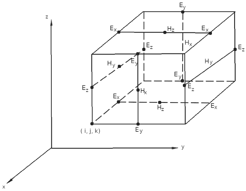
Initially FDTD algorithm has been designed by Kane Yee [6] as a technique to solve Maxwell equations in isotropic media. The fields are spatially distributed across a specific grid, so called
Yee lattice, shown in Fig. 1. Time distribution is also different for electric and magnetic fields. The electric field stored at time moments where is integer, while
the magnetic fields keep time positions.
This pattern of fields allocation might seems strange, but shows robust stability and reduces required memory [7].
As it has been shown at [6] in isotropic non-dispersive case fields can be calculated as:
(1)
The same way we obtain equations for and accounting also current .
When electric and magnetic inductions are known, we have to calculate the intensity fields ( and ) for the next time step.
The way it is implemented in MEEP [8] can be assumed as a two step procedure. First we subtract material
polarizations from the induction fields ( and ), after we divide this value by or .
The used approach allows to account material responses of different physical nature at the same time. Each non-trivial material response corresponds to a polarization.
III Recursive convolutions
The simplest case of magnetized plasma is a situation when cyclotron resonance is caused by Z-directed static magnetic field. The corresponding permittivity tensor can be found in [9]:
(2)
where
(3)
(4)
(5)
As it has been shown in [10] the corresponding electric susceptibilities can be considered as real parts of complex variables:
(6)
(7)
(8)
Corresponding polarization equations have been derived in the previous work [5]:
(9)
where index can be or .To treat polarizations as recursive convolutions and avoid expensive calculations, diagonal and off-diagonal parts are splitted into two parts each:
(10)
Both of the terms of 10 can be calculated as a recursive convolution:
(11)
(12)
Diagonal parts of the polarization calculated similar way and their recursive convolution form can be written as:
(13)
Material response to field is z-component of the polarization vector can be accounted a recursive convolution too:
(14)
(15)
(16)
To distinguish physically valuable polarization from the parts, we will rename the parts and will call them ”convolutions”:
(17)
IV Coordinate frame change
Consider two coordinate frames. The first is our old coordinates where bias static magnetic field directed along Z-axis. For simplicity sake we will consider .
The second one is a new frame where the bias field is
arbitrary directed. There is a transformation matrix changing coordinates of vectors from to . As tensor projects vector into , in
the new coordinate frame tensor should project into :
(18)
If we rewrite and using matrix:
(19)
or
(20)
Now we have to find matrix, to do this we can use Rodrigues’ rotation formula [11]:
(21)
where is a cosine between the Z axis and the bias field, s – sinus os the same angle, and is defined as:
(22)
or in our case this matrix can be written as:
(23)
while
(24)
The function (21) is not defined in a case when the sinus between and the Z-axis is 0. To overcome this we manually define two cases.
First, when directed along the Z-axis, is trivial and the matrix is identity matrix. In the second case, when is directed opposite the Z axis, described one of two possible matrices:
(25)
(26)
these matrices give the same result. For sake of certainty we will use (25).
V Implementation
As elements of tensor are formulas one can not directly use (20). Instead of that we can decompose as:
(27)
Applying (20) on matrices from decomposition (27) we obtain projection matrices:
(28)
The projection matrices (28) are generated in the constructor of ”gyroelectric-susceptibility” class.
Since a high precision 3D simulation can require billions of grid cells, memory allocation is an important task. Memory allocation algorithm is determined in ”new_internal_data” function of the class.
The function allocates 2 complex double float numbers for each grid cell for every non-zero projection matrix element. Those recursive convolutions are calculated in ”update_P” function
of ”gyroelectric-susceptibility” class. New values of the polarizations are calculated as sum of products of convolutions and according projections:
(29)
Function ”subtract_P” and the next steps are not affected by the change of coordinate system.
VI Test case
The analytical model is 9mm layer of magnetized plasma with the bias field directed along the Z-axis.
Parameters for the analytical model are chosen to be: rad/s, rad/s, and Hz.
As it has been shown in [12] transmission of a slab can be written as:
(30)
where and are the complex
Fresnel reflection and transmission amplitude coefficients for vacuum (index 1) and the plasma (index 2).
There are very strong dependence frequency of transmission for left and right circular polarized waves when we put according [9] into (30):
(31)
(32)
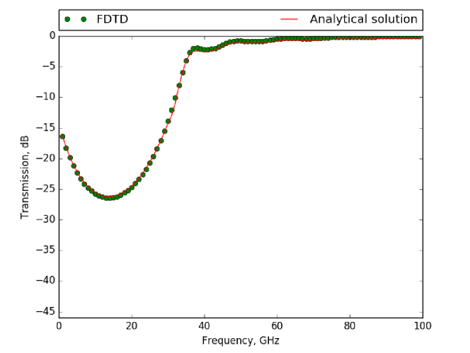
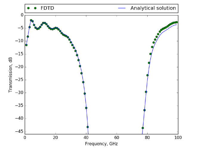
The analytical solution is compared to the FDTD calculations result in Fig.2 and Fig.3
Figure 2: Comparison of the right circular polarized electromagnetic wave transmission.Figure 3: Comparison of the left circular polarized electromagnetic wave transmission.
To test the coordinate frame change algorithm the bias field was directed opposite the Z-axis. In this case LCP and RCP transmission swapped as it should be according to the T matrix defined in
(25). The reader might substitute it into equations (28) keeping in mind that in this case T matrix is involutory.
VII Summary
A new approach of FDTD simulation of magnetized plasma media allowing to set arbitrary direction of the bias field is proposed. The implementation is based on MEEP, a widely used FDTD solver.
The simulation results for four cases compared to the analytical solutions and matched.
The source code is available on https://github.com/alexfriman/offidiagonal-meep
Acknowledgment
The author would like to thank Nikolay Shubin for the discussion on linear algebra.
References
[1] Hamidreza Ramezani, D. N. Christodoulides, V. Kovanis, I. Vitebskiy, and Tsampikos Kottos, ”PT-Symmetric Talbot Effects”, Phys. Rev. Lett., vol. 109, pp. 033902, Jul 2012
[2] Zin Lin, Hamidreza Ramezani, Toni Eichelkraut, Tsampikos Kottos, Hui Cao, and Demetrios N. Christodoulides, ”Unidirectional Invisibility Induced by PT-Symmetric Periodic Structures”, Phys. Rev. Lett., vol. 106, pp. 213901, May 2011
[3] Ali Mostafazadeh, ”Invisibility and PT-symmetry”, Phys. Rev. A, vol. 87, pp. 012103, January 2013
[4] Maryam Sakhdari, Nasim Mohammadi Estakhri, Hakan Bagci, and Pai-Yen Chen, ”Low-Threshold Lasing and Coherent Perfect Absorption in Generalized PT-Symmetric Optical Structures”, Phys. Rev. Applied, vol. 10, pp. 024030, August 2018
[5] A. V. Friman, A. A. Gorbatsevich and P. P. Sverbil, ”Finite-Difference Time-Domain Technique for Gyroelectric Material Structure Simulation Using Recursive Convolutions in Polarization,” IEEE Transactions on Antennas and Propagation, vol. 65, no. 5, pp. 2745–2747, May 2017.
[6] K. Yee, ”Numerical solution of inital boundary value problems involving Maxwell’s equations in isotropic media”, IEEE Transactions on Antennas and Propagation, vol. 14, issue 3, pp. 302–307, May 1966.
[7] A. Taflove, S.C. Hagness ”Computational Electrodynamics: The Finite-difference Time-domain Method”, Artech House, 2005.
[8] Ardavan F. Oskooi, David Roundy, Mihai Ibanescu, Peter Bermel, J.D. Joannopoulos, Steven G. Johnson, ”Meep: A flexible free-software package for electromagnetic simulations by the FDTD method”, Computer Physics Communications, vol. 181, pp. 687–702, March 2010
[9] V. Ginzburg, ”Propagation of Electromagnetic Waves in Plasma (Russian Monographs and Texts on Advanced Mathematics and Physics).”, New York, NY, USA: Gordon and Breach, 1962.
[10] F. Hunsberger, R. Luebbers, and K. Kunz, “Finite-difference time-domain analysis of gyrotropic media. I. Magnetized plasma,”, IEEE Trans. Antennas Propag., vol. 40, no. 12, pp. 1489–1495, Dec. 1992.
[11] Tadej Bajd, Matjaž Mihelj, Marko Munih, ”Introduction to Robotics”, Netherlands, Springer, 2013
[12] M. Born and E. Wolf, ”Principles of Optics: Electromagnetic Theory of Propagation, Interference, and Diffraction of Light.”, Oxford, U.K.: Pergamon Press, 1959.