Guided Graph Spectral Embedding

Abstract

Graph spectral analysis can yield meaningful embeddings of graphs by providing insight into distributed features not directly accessible in nodal domain. Recent efforts in graph signal processing have proposed new decompositions—e.g., based on wavelets and Slepians—that can be applied to filter signals defined on the graph. In this work, we take inspiration from these constructions to define a new guided spectral embedding that combines maximizing energy concentration with minimizing modified embedded distance for a given importance weighting of the nodes. We show that these optimization goals are intrinsically opposite, leading to a well-defined and stable spectral decomposition. The importance weighting allows to put the focus on particular nodes and tune the trade-off between global and local effects. Following the derivation of our new optimization criterion, we exemplify the methodology on the C. elegans structural connectome. The results of our analyses confirm known observations on the nematode’s neural network in terms of functionality and importance of cells. Compared to Laplacian embedding, the guided approach, focused on a certain class of cells (sensory neurons, interneurons or motoneurons), provides more biological insights, such as the distinction between somatic positions of cells, and their involvement in low or high order processing functions.

Network Neuroscience

Institute of Bioengineering, École Polytechnique Fédérale de Lausanne, Campus Biotech, Geneva, Switzerland Department of Radiology and Medical Informatics, University of Geneva, Geneva, Switzerland

Dimitri Van De Villedimitri.vandeville@epfl.ch

1 Introduction

Many aspects of network science relate to graph partitioning—the grouping of nodes in subgraphs—and graph embedding—their representation in a low-dimensional space that accounts for graph topology (Von Luxburg, 2007). Spectral graph theory motivates analytical methods based on the eigenvectors of fundamental graph operators, such as the adjacency and the Laplacian operators (Chung, 1997). For instance, the well-known graph cut problem can be convexly relaxed and solved by thresholding of the Laplacian eigenvector with the smallest non-zero eigenvalue, known as the Fiedler vector (Fiedler, 1989). More recently, new approaches in graph signal processing have taken advantage of the Laplacian eigenvectors to define the graph Fourier transform, which can then be used to process (i.e., filter) graph signals in the spectral domain (Shuman ., 2013; Ortega ., 2018); the spectral graph wavelet transform by Hammond . (2011) is one such example.

The Laplacian eigenvectors also provide a meaningful embedding by mapping nodes onto a line, or higher-dimensional representation, that minimizes distances between connected nodes (Belkin  Niyogi, 2003). Other well-known embedding techniques use different metrics for distance in order to assess local graph properties, ranging from simple Euclidean distance in locally linear embedding (Roweis, 2000), to shortest path in Isomap (Tenenbaum, 2000), transition probability  (Shen  Meyer, 2008), or conditional probability of an edge in t-distributed stochastic neighbor embedding (van der Maaten  Hinton, 2008). A time-dependent dynamical similarity measure has also been introduced  (Schaub ., 2018). In addition, efforts have been made to employ global properties of the graph, such as in Sammon mapping (Sammon, 1969), where a cost function including all pairwise distances is optimized. In this manner, embedding is performed while taking in consideration both local (neighborhood) and global (distant nodes) properties of the graph. However, these techniques are not aware of the network at the mesoscale: one cannot guide the embedding by giving a certain subgraph more importance while still preserving local features and global topology characteristics.

In essence, the most powerful feature of graph spectral embedding is to effectively summarize local structure across the graph into low-dimensional global patterns. This is achieved, for instance, with the recently introduced concept of graph Slepians; i.e., graph signals that are bandlimited and take into account a subset of selected nodes. Specifically, two types of Slepian designs that respectively optimize for energy concentration and modified embedded distance have been introduced (Van De Ville, 2016; Van De Ville ., 20172).

In this work, we further build on this framework by providing a simple way to guide analyses with additional flexibility. Guidance includes the selection of a given subgraph or group of nodes to study, and the ability to specify the intensity of the focus set on these selected nodes. With respect to graph Slepians, we hereby provide several extensions. First, we allow the selection process to be weighted, so that the importance of a node can be gradually changed. Second, we propose a new criterion that meaningfully combines the two existing ones; i.e., we want to maximize energy concentration and minimize modified embedded distance at the same time. Third, as we detail below, these two criteria are counteracting, and hence, we obtain stable solutions even at full bandwidth, where the original Slepian designs degenerate numerically. Fourth, we show how this criterion can be rewritten as an eigenvalue problem of an easy modification of the adjacency matrix, which can be interpreted as reweighting paths in the graph, and thus significantly simplifies the whole Slepian concept. The solution of the eigendecomposition then defines the guided spectral domain, spanned by its eigenvectors. We illustrate the proposed approach with a proof-of-concept on the Caenorhabditis elegans (C. elegans) connectome. Through spectral embedding-based visualization, we observe the effects of focusing on a specific cellular population made of sensory neurons, interneurons or motoneurons, and we reveal trajectories of these neurons as a function of focus strength.

Figure 1: Spectral embedding of the C. elegans connectome according to the eigenvectors of the Laplacian matrix with second and third smallest eigenvalues. The purpose of this work is to introduce guided spectral analysis; that is, to indicate direction by selecting a subset of nodes, and to adjust the strength of the focus set on this subset. Each colored circle in the figure depicts one C. elegans neuron. Light gray strokes link the cells that are connected by gap junctions or chemical synapses. Labels and connectivity were retrieved from Varshney . (2011).

2 Methods

2.1 Essential Graph Concepts

We consider an undirected graph with $N$ nodes, labeled $1,2,\ldots,N$. The edge weights are contained in the symmetric weighted adjacency matrix $\tilde{{\bf A}}$ with non-negative real-valued elements $\tilde{a}_{i,j}$, $i,j=1,\ldots,N$. We also assume that the graph contains no self-loops; i.e., all diagonal elements $\tilde{a}_{i,i}$ are zero. The degree matrix ${\bf D}$ is the diagonal matrix with elements $d_{i,i}=\sum_{j=1}^{N}\tilde{a}_{i,j}$. The graph Laplacian is defined as $\tilde{{\bf L}}={\bf D}-\tilde{{\bf A}}$ and can be interpreted as a second-order derivative operator on the graph. Here, we use the symmetrically normalized variants of the adjacency $\tilde{{\bf A}}$ and graph Laplacian $\tilde{{\bf L}}$ defined as ${\bf A}={\bf D}^{-1/2}\tilde{{\bf A}}{\bf D}^{-1/2}$ and ${\bf L}={\bf I}-{\bf A}$. This normalization is often used in applications to emphasize the changes in topology and not in nodal degree (De Lange ., 2014).

Let us define a graph signal as a vector of length $N$ that associates a value to each node (Shuman ., 2013). One way to recognize the importance of the Laplacian and its eigendecomposition is to consider the smoothness of a graph signal ${\bf x}$ as

$${\bf x}^{\top}{\bf L}{\bf x}=\sum_{i,j=1}^{N}a_{i,j}(x_{i}-x_{j})^{2},$$ (1)

which sums squared differences between signal values on nodes that are connected, proportionally to their link strength $a_{i,j}$. The eigenvectors of ${\bf L}$ minimize this distance that is reflected by the eigenvalues, sorted by convention increasingly as ${\lambda_{1}=0\leq\lambda_{2}\leq\ldots\leq\lambda_{N}}$. Therefore, considering the eigenvectors associated to the smallest non-zero eigenvalues provides the Laplacian embedding of the nodes that minimizes distance in a lower-dimensional space (Belkin  Niyogi, 2003). The eigenvector with the smallest non-zero eigenvalue is also known as the Fiedler vector (Fiedler, 1989), which relates to the solution of the convex relaxation of the graph cut problem (Von Luxburg, 2007).

Therefore, the eigendecomposition ${\bf L}={\bf U}{\bf\Lambda}{\bf U}^{\top}$ of the graph Laplacian is the cornerstone of spectral methods for graphs, as the eigenvectors $\{\mathbf{u}_{k}\}$, $k=1,...,N$ (columns of ${\bf U}$) play the role of graph Fourier components, and the associated eigenvalues $\{\lambda_{k}\}$, $k=1,...,N$, of frequencies (Chung, 1997). The graph Fourier transform (GFT) then provides the link between a graph signal ${\bf x}$ and its spectral coefficients given by vector $\hat{{\bf x}}$:

$${\bf x}={\bf U}\hat{{\bf x}},\text{ and }\hat{{\bf x}}={\bf U}^{\top}{\bf x}.$$

2.2 Graph Slepians

In earlier work, the combination of the concepts of selectivity and bandwidth for graph signals has been used to define “graph Slepians” (Tsitsvero ., 2016; Van De Ville, 2016; Van De Ville ., 20172); i.e., bandlimited graph signals with maximal energy concentration in the subset of nodes $\mathcal{S}$—a generalization of prolate spheroidal wave functions that were proposed fifty years ago on regular domains to find a trade-off between temporal and spectral energy concentrations (Slepian  Pollak, 1961; Slepian, 1978). The presence or absence of a node in $\mathcal{S}$ is encoded by the diagonal elements of the selection matrix ${\bf S}$; that is, we have $S_{i,i}=\delta_{i\in\mathcal{S}}$, $i=1,\ldots,N$, where $\delta$ is the Kronecker delta. The Slepian design then boils down to finding the linear combination of Laplacian eigenvectors, encoded by spectral coefficients $\hat{{\bf g}}$, within the bandlimit $W$ with maximal energy in $\mathcal{S}$, reverting to the Rayleigh quotient

$$\mu=\frac{\hat{{\bf g}}^{\top}{\bf W}^{\top}{\bf U}^{\top}{\bf S}{\bf U}{\bf W}\hat{{\bf g}}}{\hat{{\bf g}}^{\top}\hat{{\bf g}}},$$ (2)

where ${\bf W}$ is a spectral selection matrix that has $W$ ones on its diagonal followed by $N-W$ zeros. This problem can be solved by the eigendecomposition of the concentration matrix ${\bf C}={\bf W}^{\top}{\bf U}^{\top}{\bf S}{\bf U}{\bf W}$ as ${\bf C}\mathbf{\hat{g}}_{k}=\mu_{k}\mathbf{\hat{g}}_{k}$, $k=1,...,W$. The graph Slepians $\mathbf{g}_{k}={\bf U}\mathbf{\hat{g}}_{k}$, $k=1,...,W$, are orthonormal over the entire graph as well as orthogonal over the subset $\mathcal{S}$; i.e., we have $\mathbf{g}_{k}^{\top}\mathbf{g}_{l}=\delta_{k-l}$ as well as $\mathbf{g}_{k}^{\top}{\bf S}\mathbf{g}_{l}=\mu_{k}\delta_{k-l}$.

For the purpose of this work, we introduce the set of bandlimited graph signals

$$\mathcal{B}_{W}=\left\{{\bf x}|\hat{{\bf x}}={\bf W}\hat{{\bf x}}\right\},$$

such that we can then rewrite the Slepian criterion of Eq. (2) directly in the vertex domain as

$$\mu=\frac{{\bf g}^{\top}{\bf S}{\bf g}}{{\bf g}^{\top}{\bf g}}\quad\text{s.t. }{\bf g}\in\mathcal{B}_{W}.$$ (3)

An alternative Slepian design was also proposed in Van De Ville . (20172)—see also Huang . (2018), modifying the Laplacian embedded distance of Eq. (1) as follows:

$$\xi=\frac{{\bf g}^{\top}{\bf L}^{1/2}{\bf S}{\bf L}^{1/2}{\bf g}}{{\bf g}^{\top}{\bf g}}\quad\text{s.t. }{\bf g}\in\mathcal{B}_{W}.$$ (4)

The Laplacian embedded distance ${\bf x}^{\top}{\bf L}{\bf x}$ is a measure of smoothness of the vector ${\bf x}$ over the graph, which is why eigenvectors of ${\bf L}$ with increasing eigenvalues are ordered according to smoothness. Imposing the modification with the selection matrix ${\bf S}$ focuses the smoothness on a certain subgraph, notwithstanding how the signal behaves outside it. Eq. (4) can also be seen as a generalization of Laplacian embedding, since ${\bf L}^{1/2}{\bf S}{\bf L}^{1/2}$ reverts to ${\bf L}$ for the special case of ${\bf S}={\bf I}$.

It is important to realize that the eigenvalues $\{\mu_{k}\}$ of the original design reflect the energy concentration in the subset $\mathcal{S}$, while the eigenvalues $\{\xi_{k}\}$ of the alternative design correspond to a modified embedded distance that can be interpreted as a “frequency value” localized in $\mathcal{S}$, in analogy to the global GFT case. Consequently, “interesting” eigenvectors correspond to those with high $\mu_{k}$, concentrated in the subset $\mathcal{S}$, or low $\xi_{k}$, showing the main localized low-frequency trends, respectively. However, the eigendecompositions, taken individually, do not necessarily lead to eigenvectors that combine both virtues.

2.3 Guiding Spectral Embedding Using a New Criterion

We hereby propose to further generalize the Slepian design in a number of ways. First, we relax the selection matrix ${\bf S}$ to a cooperation matrix ${\bf M}$ with diagonal elements that can take any non-negative real values $m_{l}\geq 0$, $l=1,\ldots,N$. This allows to gradually change the impact of a node on the analysis, between an enhanced ($m_{l}>1$), an unmodified ($m_{l}=1$) and a reduced ($m_{l}<1$) importance with respect to the selection matrix case. Second, we combine the criteria of both already existing Slepian designs by subtracting the modified embedded distance from the energy concentration:

$$\zeta=\mu-\xi=\frac{{\bf g}^{\top}{\bf M}{\bf g}-{\bf g}^{\top}{\bf L}^{1/2}{\bf M}{\bf L}^{1/2}{\bf g}}{{\bf g}^{\top}{\bf g}}\quad\text{s.t. }{\bf g}\in\mathcal{B}_{W}.$$ (5)

Third, we remove the bandlimit constraint and allow ${\bf g}$ to be any graph signal, which is an operational choice due to the joint optimization of both criteria, as will be illustrated and discussed later on.

Using the Taylor series approximation of the square root function, we derive ${\bf L}^{1/2}$ in terms of the adjacency matrix ${\bf A}$:

$${\bf L}^{1/2}=({\bf I}-{\bf A})^{1/2} = {\bf I}-\frac{1}{2}{\bf A}-\frac{1}{8}{\bf A}^{2}-\frac{1}{16}{\bf A}^{3}-\ldots$$ (6)

$$= {\bf I}-\sum_{k=1}^{\infty}c_{k}{\bf A}^{k},$$ (7)

with $c_{k}=\frac{(2k)!}{2^{2k}(k!)^{2}(2k-1)}.$ Details on the series expansion are discussed in Section 3.3. We can then further rewrite the internal part of the criterion (5) as

$${\bf M}-({\bf I}-{\bf A})^{1/2}{\bf M}({\bf I}-{\bf A})^{1/2} = \sum_{k=1}^{\infty}c_{k}\left({\bf M}{\bf A}^{k}+{\bf A}^{k}{\bf M}\right)$$ (8)

$$-\sum_{k_{1}=1}^{\infty}\sum_{k_{2}=1}^{\infty}\left(c_{k_{1}}c_{k_{2}}\right){\bf A}^{k_{1}}{\bf M}{\bf A}^{k_{2}}.$$

By convention, the associated eigenvalues are sorted in decreasing order. Based on the fact that eigenvalues of the symmetric normalized Laplacian are greater or equal to 0 and lower or equal to 2, one can derive ${m_{\text{max}}\geq\zeta_{1}\geq\zeta_{2}\geq\ldots\geq-2m_{\text{max}}}$, where $m_{\text{max}}$ is the highest cooperation value appearing in ${\bf M}$, using bounds from Corollary 2.4 in  Lu  Pearce (2000).

In what follows, we will be considering the linear and quadratic approximations of the new criterion’s eigenvalues:

$$\zeta_{\text{lin}} = \frac{{\bf g}^{\top}\left(\frac{{\bf M}{\bf A}+{\bf A}{\bf M}}{2}\right){\bf g}}{{\bf g}^{\top}{\bf g}}$$ (9)

$$\zeta_{\text{quad}} = \frac{{\bf g}^{\top}\left(\frac{{\bf M}{\bf A}+{\bf A}{\bf M}}{2}+\frac{{\bf M}{\bf A}^{2}+{\bf A}^{2}{\bf M}}{8}-\frac{{\bf A}{\bf M}{\bf A}}{4}\right){\bf g}}{{\bf g}^{\top}{\bf g}}.$$ (10)

Interestingly, the combination of both existing Slepian criteria leads to the emergence of the adjacency matrix ${\bf A}$ as the key player in our new formalism. In fact, when the cooperation matrix is the identity matrix, the criterion reverts to the eigendecomposition of ${\bf A}$ itself.

Let us now interpret the impact of the cooperation weights: obviously, an element $a_{i,j}$ of the adjacency matrix contains the weight of a direct path from $i$ to $j$. The linear approximation $\zeta_{\text{lin}}$ reweights such a direct path with the average $(m_{i}+m_{j})/2$ of the cooperation weights that are attributed to nodes $i$ and $j$, as illustrated in Fig. 2A (left half). Notice that paths where only one node has a cooperation weight equal to $0$ are still possible, as the other cooperation weight is then simply divided by two.

As for the quadratic approximation, it takes into account length-2 paths between nodes $i$ and $j$. For instance, the sum of all length-2 paths between $i$ and $j$ can be read out from the squared adjacency matrix:

$$[{\bf A}^{2}]_{i,j}=\sum_{l=1}^{N}a_{i,l}a_{l,j}=\left<\mathbf{a}_{i,\cdot},\mathbf{a}_{\cdot,j}\right>,$$

where the inner product reveals the kernel interpretation of the length-2 walk matrix. Therefore, as illustrated in Fig. 2A (right half), the term

$$[{\bf M}{\bf A}^{2}+{\bf A}^{2}{\bf M}]_{i,j}=(m_{i}+m_{j})\sum_{l=1}^{N}a_{i,l}a_{l,j}$$

reweights all length-2 paths by the summed cooperation weight between the start and end nodes, while subtracting the term

$$[{\bf A}{\bf M}{\bf A}]_{i,j}=\sum_{l=1}^{N}m_{l}a_{i,l}a_{l,j}$$

penalizes the path according to the cooperation weight of node $l$ through which it passes.

Analogously, the term ${\bf A}^{k}$ in the criterion introduces modifications of $k$-length paths in the graph. However, for $k>N$, reweighting reduces to modifications of lower-length paths. The Cayley-Hamilton theorem implies that for every matrix ${\bf A}$ of size $N\times N$, the matrix ${\bf A}^{N}$ can be written as a linear combination of matrices ${\bf A}^{k}$ for $k=0,1,\ldots N-1$. By induction, it holds that ${\bf A}^{k}$ for every $k>N$ can also be written as a linear combination of the same set of $N$ matrices. Hence, modifications of paths longer than $N-1$ can be seen as a linear combination of additional modifications of paths of length 0 to $N-1$.

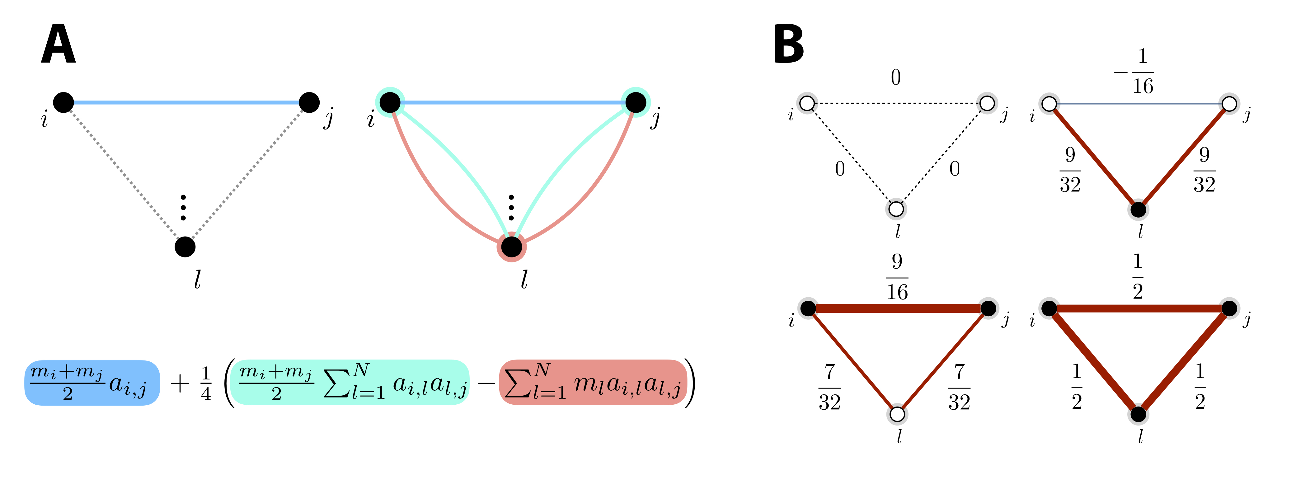
Figure 2: A. In the case of two nodes $i$ and $j$, the average of their cooperation weights yields the multiplying factor for $a_{i,j}$ (blue term). When a third node $l$ is added, the difference between average cooperation weight between nodes $i$ and $j$ (light blue term), and the cooperation weight of node $l$ (salmon term), multiplies the length-2 path and then also contributes to the output entry. B. In an example three-node network, output entries for different examples where cooperation weights are either set to $0$ (white nodes) or to $1$ (black nodes). Edge thickness is proportional to the output entry weight. Red strokes denote positive edge values, while blue strokes highlight negative edge values. All non-zero entries of the normalized adjacency matrix of the example network equal 1/2.

3 Mathematical Considerations

This section provides mathematical foundations supporting the methods and the results presented in this work. We start by discussing the link between the selection matrix and the eigenspectrum associated to the energy concentration criterion, and the relationship with the modified embedded distance criterion, using full bandwidth. Then, we provide a formal justification of the Taylor series approximation of the square root matrix function used in Eq. (6), and discuss the error associated to this approximation.

3.1 Eigenspectrum associated to the energy concentration criterion

For full bandwidth, the concentration matrix is defined as ${\bf C}={\bf U}^{\top}{\bf S}{\bf U}$, where ${\bf U}$ is the matrix whose columns are eigenvectors of the graph Laplacian, and ${\bf S}$ is a diagonal selection matrix. Hence, the eigendecomposition of ${\bf C}$ is trivial: its eigenvectors are the rows of ${\bf U}$, and the eigenvalues of ${\bf C}$ correspond to the diagonal entries of ${\bf S}$, as can be seen from Fig. 3A for $W=279$.

3.2 Eigenspectrum associated to the modified embedded distance criterion

We show that for full bandwidth, the number of zero eigenvalues of the modified embedded distance matrix, denoted $z_{\lambda}$, is lower-bounded by the number of zeros on the diagonal of the selection matrix, denoted $z_{S}$. To see this, consider the following decomposition of the modified embedded distance matrix ${\bf C}_{emb}$:

$${\bf C}_{emb}={\bf L}^{1/2}{\bf S}{\bf L}^{1/2}=\sum_{k=1}^{N-z_{S}}s_{i_{k}}l_{i_{k}}l_{i_{k}}^{\top},$$

where $i_{k}$ is the index of the $k^{\text{th}}$ non-zero entry of the selection matrix ${\bf S}$, and $l_{i_{k}}$ denotes the $i_{k}$^th column vector of the matrix ${\bf L}^{1/2}$. From this expression, it can be seen that the rank of ${\bf C}_{emb}$ is at most $N-z_{S}$ and hence, $z_{\lambda}\geq z_{S}$. Equality holds when the set of vectors $\{l_{i_{k}}\}$ corresponding to the non-zero entries of ${\bf S}$ are linearly independent. This is the case for connected graphs, as any subset (with cardinality strictly less than $N$) of the columns of ${\bf L}^{1/2}$ is linearly independent. This relationship is observed in Fig. 3B for $W=279$.

3.3 Taylor series of matrix-valued functions

The Taylor expansion of ${\bf L}^{1/2}$ proposed in Eq. (6) is derived using the scalar Taylor series of $f(x)=\sqrt{x}$ evaluated around the point $a=1$:

$$\sqrt{x}=1+\sum_{k=1}^{\infty}t_{k}(x-1)^{k},$$

where $t_{k}=\frac{(-1)^{k-1}(2k)!}{2^{2k}(k!)^{2}(2k-1)}$ and $x\in\mathbb{R},x>0$. The square root matrix of ${\bf L}$ then writes:

$${\bf L}^{1/2} = {\bf U}_{L}{\bf\Lambda}^{1/2}_{L}{\bf U}_{L}^{\top}$$

$$= {\bf U}_{L}\begin{bmatrix}1+\sum_{k=1}^{\infty}t_{k}(\lambda_{1}-1)^{k}&&\\ &\ddots&\\ &&1+\sum_{k=1}^{\infty}t_{k}(\lambda_{N}-1)^{k}\\ \end{bmatrix}{\bf U}_{L}^{\top}$$

$$= {\bf U}_{L}({\bf I}+\sum_{k=1}^{\infty}t_{k}({\bf\Lambda}_{L}-{\bf I})^{k}){\bf U}_{L}^{\top}.$$

Since the Laplacian and adjacency matrices are normalized, their eigenvalues verify ${\bf\Lambda}_{L}={\bf I}-{\bf\Lambda}_{A}$ and their eigenvectors are equal (${\bf U}_{L}={\bf U}_{A}$) when ordered following increasing and decreasing eigenvalues, respectively. The previous equation finally reduces to:

$${\bf L}^{1/2} = {\bf I}+{\bf U}_{A}(\sum_{k=1}^{\infty}t_{k}(-{\bf\Lambda}_{A})^{k}){\bf U}_{A}^{\top}$$

$$= {\bf I}+\sum_{k=1}^{\infty}(-1)^{k}t_{k}{\bf U}_{A}{\bf\Lambda}_{A}^{k}{\bf U}_{A}^{\top}$$

$$= {\bf I}-\sum_{k=1}^{\infty}c_{k}{\bf A}^{k},$$

where $c_{k}=\frac{(2k)!}{2^{2k}(k!)^{2}(2k-1)}$, which is the expression used in Eq. (6).

Truncation of the Taylor series of a function $f(x)$ to a finite upper bound on $k\leq K$ leads to an approximation error which can be estimated by the Lagrange form of the remainder

$$R_{K}(x)=\frac{f^{(K+1)}(y)}{(K+1)!}(x-1)^{K+1},$$

where the $(K+1)^{\text{th}}$ derivative is evaluated at the point $y$ found between $x$ and $1$. On the other hand, since the eigenvectors forming ${\bf U}_{L}$ are unit-norm vectors, the distance $d_{K}$ between a finite sum approximation of ${\bf L}^{1/2}$ and the true square root of the matrix is bounded as:

$$d_{K}=||{\bf L}^{1/2}-({\bf I}-\sum_{k=1}^{K}c_{k}{\bf A}^{k})||_{F}\leq\sum_{i=1}^{N}|R_{K}(\lambda_{i})|,$$

where $||\cdot||_{F}$ denotes the Frobenius norm. In the case of a first order Taylor approximation ($K=1$), we get:

$$d_{1}\leq\sum_{i=1}^{N}\frac{|f^{(2)}(y_{i})|}{2!}(\lambda_{i}-1)^{2}.$$

The eigenvalues $\lambda_{i}$ range from $0$ to $2$, and all contribute to the total approximation error $d_{1}$, with eigenvalues further from $1$ contributing more. Since the second-order derivative of the square root function increases as its argument approaches $0$, the most contributing factors of the error derive from Taylor approximation terms with near-zero eigenvalues. Hence, graphs whose Laplacian spectrum exhibits higher eigengaps in the lower band tend to have lower approximation error.

Finally, the Frobenius distance $d_{K,M}$ between the true proposed criterion ${\bf M}-{\bf L}^{1/2}{\bf M}{\bf L}^{1/2}$ and its approximation using a $K$^th-order Taylor approximation of ${\bf L}^{1/2}$ verifies:

$$d_{K,M}\leq d_{K}||{\bf M}||_{F}d_{K},$$

where $||{\bf M}||_{F}$ corresponds to the Frobenius norm of the cooperation matrix. Hence, the upper bound on $d_{K,M}$ reduces as the nodes are given less importance; i.e., when the cooperation values get closer to 0.

4 Results

The C. elegans worm is an intensely studied model organism in biology. In particular, the wiring diagram of its 302 neurons has been carefully mapped during a long and effortful study (White ., 1986). Here, we use the graph that summarizes data from 279 somatic neurons (unconnected and pharyngeal neurons were excluded from the full diagram of 302 neurons), and combined connectivity from chemical synapses and gap junctions (Chen ., 2006). The binary adjacency matrix ${\bf A}_{bin}$ with edge weights 0 or 1 has been symmetrically normalized with the degree matrix ${\bf D}$ into ${\bf A}={\bf D}^{-1/2}{\bf A}_{bin}{\bf D}^{-1/2}$, as described in Section 2.1. We retrieved the type of each neuron (sensory neuron, interneuron or motoneuron) from the WormAtlas database (http://www.wormatlas.org/).

In their modeling work, Varshney . (2011) studied network properties of the worm connectome using different approaches, including Laplacian embedding. In particular, the topological view generated by mapping nodes on the first two eigenvectors with smallest non-zero eigenvalues already reveals interesting network organization (see Fig. 1). The horizontal dimension (${\bf u}_{2}$) mainly distinguishes the motoneurons from the head (right green circles) and from the ventral cord (left green circles). The vertical dimension (${\bf u}_{3}$) reflects information flow from sensory neurons and interneurons of the animal’s head (top) to the nerve ring and ventral cord circuitries (bottom).

4.1 Eigenvalues of Different Criteria

To illustrate the eigenvalues obtained with the existing Slepian designs, as well as the newly proposed criterion, we considered the 128 motoneurons and “unselected” them by setting their respective entries in ${\bf S}$ to $0$. We applied the original, concentration-based Slepian design for different bandwidths $W=100,150,200,279$, the latter corresponding to full bandwidth. The eigenvalues $\mu_{k}$, which reflect energy concentration in the 151 remaining neurons, are shown in Fig. 3A. The characteristic behavior of classical Slepians is preserved for the graph variant; i.e., eigenvalues cluster around $1$ and $0$ for well and poorly concentrated eigenvectors, respectively, and the phase transition occurs more abruptly at higher bandwidth. For full bandwidth, perfect concentration becomes possible, and the problem degenerates in retrieving two linear subspaces of 151 and 128 dimensions spanned by eigenvectors with concentration $1$ and $0$, respectively (see Section 3.1 for a proof on the number of distinct eigenvalues). In practical terms, for high but not full bandwidth, the “interesting” eigenvectors with large concentration correspond to the part indicated by the green area on the plot, and become numerically indistinguishable. A few indicative examples of Slepian vectors across bandwidths are displayed in Supplementary Fig. S1C.

Next, we applied the modified Slepian design inspired by the Laplacian embedded distance. As shown in Fig. 3B, the eigenvalues $\xi_{k}$ reflect the modified embedded distance, which we now want to minimize. For increasing bandwidth (darker curves), its smallest values can be made lower; however, the subset of nodes with $S_{i,i}$ entries set to $0$ is also described by eigenvectors with small eigenvalues. This becomes even clearer at full bandwidth, a case for which a subspace of 128 dimensions spanned by eigenvectors with a modified embedded distance of $0$ is retrieved, as indicated by the green area in Fig. 3B and explicitly demonstrated in Section 3.2. Some examples of Slepians across bandwidths can be seen in Supplementary Fig. S1D.

The degeneracies of the Slepian designs at full bandwidth are instructive about the opposing effects of maximizing energy concentration and minimizing modified embedded distance; i.e., the subspaces indicated by the green areas in Figs. 3A and B, which are optimal for the corresponding criteria, are actually different ones, representing signals on sensory and interneurons (151 nodes) on the one hand, and on motoneurons (128 nodes) on the other hand (compare Supplementary Figs. S1C and D, first rows). This leads us to the eigenvalues $\zeta_{k}$ of the proposed criterion, as shown in Fig. 3C (black curve).

The maximum eigenvalue peaks close to $1$, a case reflecting jointly high equivalent $\mu_{k}$ (blue curve) and low equivalent $\xi_{k}$ (purple curve); i.e., a high energy concentration at the same time as a low modified embedded distance (low localized graph frequency) within $\mathcal{S}$. The low amount of such solutions shows that it is difficult to conceal high energy concentration and small modified embedded distance.

As values of $\zeta_{k}$ decrease, we first observe a rise in modified embedded distance (eigenvectors remain reasonably concentrated within $\mathcal{S}$, but rapidly exhibit a larger localized graph frequency), and then a decrease of both $\mu_{k}$ and $\xi_{k}$, which indicates that eigenvectors become less concentrated within the subset of interest. Afterwards, we observe a regime in which both quantities are null at the same time; that is, a subspace spanned by eigenvectors that are fully concentrated outside $\mathcal{S}$. Notice that this set of eigenvectors is now “pushed away” from the meaningful low $\xi_{k}$ ones, and lie in the middle of the spectrum. Finally, the sign of $\zeta_{k}$ switches, and the right hand side of Fig. 3C denotes eigenvectors of increasing concentration within $\mathcal{S}$ and localized graph frequency, the latter effect dominating over the former.

Interestingly, computing the eigenspectrum using a linear approximation of the criterion matrix (Fig. 3D, light brown curve) leads to very similar results, which only slightly vary for the largest eigenvalues. When the approximation order is increased up to 20 (increasingly dark brown curves), this low error further diminishes, although a mild difference remains with the ground truth. Inspection of the Slepian vectors related to several locations of the eigenspectrum (Supplementary Fig. S2) confirmed that the only salient differences actually involved the first Slepian vector (largest eigenvalue one).

Figure 3: Plots of eigenvalues obtained using different Slepian criteria: (A) energy concentration $\mu$, (B) modified embedded distance $\xi$, and (C) our new proposed criterion $\zeta$. For the first two cases, in which the design depends on a bandwidth parameter, eigenvalue spectra are plotted for $W=100$, $150$, $200$ and $279$ with increasingly lighter blue or purple shades, respectively. In the full bandwidth case, the shaded green areas highlight eigenvalues linked to optimal solutions of the respective criteria (see Sections 3.1 and 3.2 for the associated mathematical derivations). In the third case, equivalent $\mu$ and $\xi$ eigenspectra are plotted in blue and purple on top of the $\zeta$ one. The full $\zeta$ eigenspectrum is also compared to approximations obtained through Taylor series of increasing order (D), from linear to order 20, as depicted by increasingly darker brown curves. The two smaller plots are insets sampled at the start and at the end of the main plot, respectively.

4.2 Topology Revealed by Guided Spectral Analysis

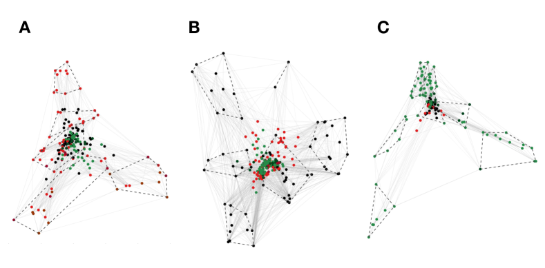
Figure S4: Clusters derived by repeated k-means clustering of the focused nodes in the case of sensory neurons (A), interneurons (B) or motoneurons (C). The optimal number of clusters was estimated with the Silhouette approach. Nodes constituting the border of each cluster’s convex hull are connected by a dashed black line to visualize the clusters.

We now guide the spectral analysis to focus on the three different types of neurons. For instance, when focussing on the role of the sensory neurons, we gradually decrease the cooperation weights of interneurons and motoneurons from $1$ to $0$. For each setting, we then visualize the topology revealed by the guided analysis by projecting the nodes on the eigenvectors with the second and third largest eigenvalues. We build the trajectory of each node through this two-dimensional embedding, after applying the Procrustes transform (Schönemann, 1966) to compensate for any irrelevant global transformations. As a complementary visualization, note that we provide the start, intermediate and end points of each trajectory as separate figures in Supplementary Fig. S3. Finally, k-means clustering was performed on the nodes in focus at the end point embedding of trajectories, producing sets of clusters given in Supplementary Fig. S4 and Supplementary Tables 1-3 (see Section 6.1 for details). Example visualizations when resorting to different Slepian vectors are provided in Supplementary Fig. S5.

In Figs. 4A and B, the trajectories are depicted when focussing on the sensory neurons by attributing cooperation weights to the other types of neurons ranging from $1$ to $0.5$, and from $0.5$ to $0$, respectively. During the first half (Fig. 4A), the network organization is only slightly altered with respect to the initial view of Fig. 1; i.e., the sensory neurons move slightly more to the periphery, while the interneurons and motoneurons move to the origin. In the second part of the trajectory (Fig. 4B), a major split occurs in the bottom right branch of Fig. 4A between the left and right versions of a whole series of neurons, while the bottom left branch neurons move back to the center of the coordinate frame. The cell types found in the top branch are amphid neurons, whereas the rest of the sensory neurons split into their left and right counterparts located in the left and right bottom branches. The clusters found by the k-means approach (see Supplementary Table 1) include a group of $5$ bilateral amphid neurons (AWA, AWC, ASE, ASI and AFD; cluster C₃) and $6$ other clusters, 2 of which span the bottom left and right sub-branches (clusters C₅ and C₂).

As described in Section 2.3, since paths through nodes with cooperation weights set to 0 are still considered by the proposed criterion, the embedding focusing on a particular subtype of neurons can still include functionally distinct cells as clearly standing out in the visualization. For instance, in addition to the above clustering of sensory neurons in Fig. 4B, we notice the segregation of the bilateral RIP interneurons towards the left and the right branch. This shows that the embedding does not neglect nodes outside the focus, even when their cooperation weight is set to 0.

Figure 4: Focussing on the sensory neurons by reducing the cooperation weights of the interneurons and motoneurons (A) from $1$ to $0.5$, and (B) from $0.5$ to $0$. The trajectory of a neuron is represented by a colour change from light to dark tones, and dots represent final positions. Note that the starting configuration in (A) is identical to the representation in Fig. 1. Cells are labeled according to Varshney . (2011).

In Figs. 5A and B, we then focus on the interneurons by reducing the cooperation weights of sensory neurons and motoneurons in two steps. As expected, the interneurons move towards the periphery. Their organization does not seem to be dominated by left versus right variants, as we found for sensory neurons, but rather by a set of well-defined clusters related to their functional involvement in the C. elegans neuronal circuitry (see Supplementary Table 2): in the first quadrant, we find the isolated AIA bilateral pair (cluster C₄). Moving clockwise, a larger cluster of neurons includes the bilateral AIY, AIZ, AIN, AIB, RIA, RIB, AUA and the single neurons RIR and RIH (cluster C₃). Next we find a cluster including AVE, AVK, RIG, PVT, DVA and other neurons located closer to the origin of Fig. 5 (cluster C₅), before reaching another large ensemble of neurons including the bilateral AVA, AVD, LUA, PVC, PVW, and the single neuron PVR (cluster C₆). Moving back upwards, cluster C₁ contains the bilateral AVB, AVJ, BDU, the single neuron AVG, and PVPR, whose left counterpart PVPL belongs to cluster C₅, thus standing as the only bilateral pair of neurons split into different clusters. Finally, we reach the last group of cells containing the bilateral RIF, AVH, AIM, PVQ and AVF (cluster C₂).

Figure 5: Focussing on the interneurons by reducing the cooperation weights of the sensory neurons and motoneurons (A) from $1$ to $0.5$, and (B) from $0.5$ to $0$. The trajectory of a neuron is represented by a colour change from light to dark tones, and dots represent final positions. Note that the starting configuration in (A) is identical to the representation in Fig. 1. Cells are labeled according to Varshney . (2011).

Finally, in Figs. 6A and B, the organization of motoneurons is examined. Already in the first step (Fig. 6A), when reducing the cooperation weights of the sensory and interneurons from $1.0$ to $0.5$, we observe much stronger changes than in the previous cases. In particular, the initial organization completely collapses and the left branch of the motoneurons spreads out. This branch then develops into a peripheral organization when further decreasing the cooperation weights (Fig. 6B), with three main subsets of neurons and ambiguous positioning of the cell DVB between the left and the right bottom branches. K-means clustering into optimal cell groups captured this architecture into $7$ smaller clusters (Supplementary Table 3): clusters C₄ and C₇ spanned top neurons, clusters C₂ and C₃ included the bottom left branch neurons, and clusters C₅ and C₆ contained the bottom right branch cells.

Figure 6: Focussing on the motoneurons by reducing the cooperation weights of the sensory neurons and interneurons (A) from $1$ to $0.5$, and (B) from $0.5$ to $0$. The trajectory of a neuron is represented by a colour change from light to dark tones, and dots represent final positions. Note that the starting configuration in (A) is identical to the representation in Fig. 1. Cells are labeled according to Varshney . (2011).

5 Discussion

5.1 Beyond Original Slepian Designs

The originality of our approach lies in providing a new and simple way to guide graph spectral analysis. Inspired by graph Slepians, we propose a novel criterion that combines energy concentration and modified embedded distance, taking into account cooperation weights that can gradually increase or decrease the importance of selected nodes. The new criterion lets the adjacency matrix emerge as the central graph operator, instead of the Laplacian, and is operational at full bandwidth.

This is surprising at first sight, because neither of the conventional Slepian criteria is practical without the bandlimit constraint. For the energy concentration with binary cooperation weights, as shown in Fig. 3A for an illustrative example on the C. elegans connectome, full bandwidth leads to two eigenvalues ($1$ and $0$), the dimensionality of the corresponding subspaces being the number of nodes with cooperation weight $1$ and $0$, respectively. For the modified embedded distance, as shown in Fig. 3B, full bandwidth creates a subspace with eigenvalue $0$ of dimensionality equal to the number of nodes with cooperation weight $0$. Therefore, subtracting both criteria leads to opposing objectives; i.e., at full bandwidth, an energy concentration of $1$ encodes the subspace for nodes with weight $1$, while a modified embedded distance of $0$ encodes the subspace for nodes with weight $0$.

The obtained eigenspectrum for the new criterion, shown in Fig. 3C, illustrates that only a few eigenvectors are able to combine high energy concentration with low modified embedded distance, a counterbalance that can be further revealed by measuring $\mu$ and $\xi$ separately for these new eigenvectors. Such a large eigengap is also good news for numerical computation of the leading eigenvectors for large graphs when relying upon efficient large-scale solvers (Lehoucq  Sorensen, 1996) implemented in widely available software libraries such as ARPACK.

Intriguingly, the approximation error was already low using a linear approximation, and did not noticeably decrease further, except for the first Slepian vector, when resorting to higher-order terms (see Fig. 3 and Supplementary Fig. S2). Modifying the importance of a node via the corresponding cooperation value affects all-length paths through that node according to the series expansion from Eq. (8), where the power of ${\bf A}$ in each term corresponds to the affected path length. Once we restrict the criterion to a linear approximation, the only paths whose importance is changed are those of length 1. This does not mean that other paths are not included in the graph analysis, but rather that they are included with their original (unmodified) effect on the topology. Low error of linear approximation suggests that the highest percentage of topological importance of a node falls into the importance of its length-1 paths. Further, a slightly higher error at eigenvectors with the highest $\zeta$ may be explained similarly: not modifying higher order paths produces greater error at these eigenvectors because of their increased relative importance due to the fact that high $\zeta$ eigenvectors tend to be very smooth (even approaching a constant signal); thus, in order to even out the values at all nodes in the process, one needs to ”reach” far enough.

The proposed criterion should not be confused with the Sobolev norm that is sometimes used to regularize graph signals (Mahadevan  Maggioni, 2006). Specifically, in the case of ${\bf M}={\bf I}$, our criterion of Eq. (5) applied to ${\bf g}$ reverts to ${\bf g}^{\top}{\bf g}-{\bf g}^{\top}{\bf L}{\bf g}$, whereas the Sobolev norm of ${\bf g}$ reads ${\bf g}^{\top}{\bf g}+{\bf g}^{\top}{\bf L}{\bf g}$. The difference in the sign of the second term introduces significantly distinct optimization goals regardless of the apparent similarity of the two expressions.

As for future extensions of our approach, one could envisage to dig into the relationship with graph uncertainty principles (Agaskar  Lu, 2013; Tsitsvero ., 2016; Teke  Vaidyanathan, ), to consider statistical resampling for graphs (Pirondini ., 2016), or to focus on the discovery of hierarchical graph structure (Arenas ., 2008; Irion  Saito, 2014) by gradual refinement of the subgraph. The design could also be extended to directed graphs using recent extensions of spectral decompositions in this context (Sandryhaila  Moura, 2013; Mhaskar, 2018).

5.2 Gaining Insights on C. elegans

The application of our newly developed approach to the C. elegans connectome enabled to confirm past findings from the literature, and to shed light on additional cellular targets and groupings that may deserve further experimental analyses. At the level of sensory neurons (Fig. 4, Supplementary Fig. S3A and Supplementary Fig. S4A), seven clusters were extracted, collectively accounting for the three branches evident in Fig. 4: the top branch made of twelve (including the thermosensor AFD) pairs of amphid neurons (at y-coordinate greater than $0.04$), and other cells split into the left and right bottom branches. Interestingly, one of the clusters found by k-means included five pairs of bilateral amphid neurons: AWA and AWC involved in odortaxis (Bargmann ., 1993; Li ., 2012), the thermosensor AFD (Mori  Ohshima, 1995), and ASE and ASI implicated in chemotaxis (Bargmann  Horvitz, 1991; Luo ., 2014). These neurons act as low-order sensors, whose extraction as a separate cluster inside the amphid group may suggest new information worth further exploration.

The lower branches in Fig. 4 split the neurons into their right and left counterparts, thus extracting relevant somatic information. These neurons act as higher-order sensing apparatus as compared with amphid neurons: IL1 and OLQ have jointly been implicated in the worm foraging response (Hart ., 1995); CEP and ADE are involved in the response upon food sensing (Sawin ., 2000); URX, URY and OLL are linked to the reproductive drive (Barrios ., 2012), and so on. The split between low and high order sensing is summarized in Fig. 7A.

Further inspection of the branches (Supplementary Fig. S6A) showed that the left-right segregation involved chemical synapses, but not gap junctions. Also, Supplementary Fig. S5 (second row) shows that for higher-order Slepian vectors (fourth and fifth), additional contributors emerge, such as the bilateral PHA/PHB. This suggests that the approach finds different subgroups of higher-order sensory neurons depending on the choice of the embedding eigenvectors. The biological/functional intepretation of the exact clusters asks for a more detailed analysis of the subgroups of neurons. Finally, the emergence of RIP interneurons in the embedding (Fig. 4) points towards an important role of the sensory neurons yet to be explained, possibly in connection with their presynaptic inputs from IL1 (White ., 1986).

Turning to interneurons (Fig. 5, Supplementary Fig. S3B and Supplementary Fig. S4B), we notice a trend of grouping neurons at the same command-chain level. Starting from the top of Fig. 5, we find AIA, AIB, AIY and AIZ jointly known for their role on locomotory behaviour and acting as a first-relay drives (Wakabayashi ., 2004; Gray ., 2005). Moving clockwise, we find RIA and RIB acting as second-layer intermediates, and further on, neurons such as AVE, and in the next cluster AVAL and AVD, all being command interneurons (Hobert, 2003; Haspel ., 2010; Kawano ., 2011). The trend of following the locomotory pathway clockwise in the embedding space suggests that the approach targets relevant information about the neural system. However, the exact compact clusters in Supplementary Fig. S4B need further elaboration. Some of the interesting findings worth exploring would be the unexplained grouping of the scarcely studied RIR neuron (Hobert ., 2002) with the cluster of cells including AIB and AIY, or the grouping of PVR and LUA (Chalfie ., 1985; Wicks  Rankin, 1995) with locomotion-regulating neurons such as AVD and AVA.

Figure 7: Summary of the main functions operated by the sensory neurons (A), interneurons (B) and motoneurons (C) unraveled by guided spectral analysis. Clusters of neurons discussed in Section 5.2 are delineated and color coded according to their main roles: this may be in sensing (thermosensation in red, olfactory sensation in yellow, chemosensation in green and mechanosensation in blue), higher-order functions (reproduction in pink, food responses in brown), or locomotion (from first cellular relays to effector motoneurons in increasingly darker shades of gray). A gradient in the color coding indicates that more than one function is performed by neurons from a given cluster. Neurons that could not be clearly related to the rest of the unraveled circuitry are encircled in white.

Considering motoneurons (Fig. 6, Supplementary Fig. S3C and Supplementary Fig. S4C), the embedding positions fit somatic location (see Supplementary Fig. S7): a spiral beginning at the origin, turning right, then moving clockwise and ending in the top branch follows the postero-anterior direction. This confirms that the approach has extracted meaningful information. However, the exact split between the three branches as well as the k-means clustering into the seven ensembles remains unclear, since, from preliminary explorations, we find both A-type and B-type cholinergic motoneurons and the inhibitory D-type motoneurons in all clusters. Finally, DVB deserves further attention (Schuske ., 2004) due to its isolated location between the two bottom branches.

In Fig. 6B, two sensory nodes stick out the furthest away from the center; i.e., towards the lower left and right branches of motoneurons. These are PVD and PHC neurons, responsible for nociceptive mechano- and thermosensation, respectively. The locations of these nodes in the embedding may be linked to the fact that harmful nociceptive stimuli induce a locomotory response. As in the case of RIP interneurons emerging in the focused embedding of sensory neurons, we once again confirm the ability of the proposed approach to extract important nodes even when their cooperation weight was initially set to 0.

In summary, as illustrated in Fig. 7, all three types of neurons found in the C. elegans nematode could be arranged in a meaningful hierarchy thanks to the introduced guided graph spectral embedding. Sensory neurons were separated between first-order and higher-order sensors. Different levels of processing of motor functions were distinguished (see the gradient from white to dark gray tones going clockwise in Fig. 7B), with the eventual recruitment of motoneurons, which have been separated on the basis of somatic location. Future analyses will allow the study of different types of neurons through more elaborate combinations of focused nodes. In addition, it will be interesting to see whether future experimental work can shed light on some of the neurons that were extracted here without being yet extensively documented in the literature, such as AVKL or RIR.

5.3 Perspectives for Future Uses

The proposed graph embedding provides a simple, yet powerful approach to visualization and, if combined with clustering techniques, to the extraction of meaningful subgraphs from any graph-modeled dataset. In neuroimaging, focusing on a specific subgraph of interest (by setting the appropriate cooperation values) can direct research onto clinically relevant concepts, such as the medial temporal lobe and limbic structures for human brain imaging studies comparing healthy controls and Alzheimer patients (Krasuski ., 1998). Be it using the structural or the functional connectome for analyses (Contreras ., 2015), features such as cluster size and/or the inclusion of specific nodes (brain regions) in a cluster may become biomarkers for an early diagnosis or prediction of the disease.

Furthermore, graph modeling of the human brain is frequently employed to extract important nodes/brain regions and to identify their topological roles, such as a provincial/connector hubs suggesting clinically significant functional roles (van den Heuvel  Sporns, 2013). Doing so requires the use of diverse node centrality measures, such as degree or betweenness centrality. On the other hand, entries of the proposed Slepian eigenvectors may be interpreted as higher-order spectral centrality measures relative to the focused subgraph, and for the special case ${\bf M}={\bf I}$, the eigenvector corresponding to the highest positive eigenvalue reverts to the eigenvector centrality (M. Newman, 2010). Hence, if clustering of a dataset based on the proposed embedding coordinates reveals nodes distant from the rest of the graph, it is suggested that those nodes exhibit a hub-like role when the focused subgraph is considered more important than the rest of the graph. For example, the AIA pair in the discussed C. elegans example emerges as a separate cluster in Fig. 5 and Supplementary Fig. S4B, where the focus is set on interneurons. Its role as a hub can be confirmed by the high number of connections to the set of amphid neurons, and a small number of connections to the other cells, as compared to the rest of the interneurons. Identification of hubs and/or peripheral nodes with respect to other similar type nodes may lead to a better understanding of the functional role of both neurons and brain regions, depending on the inspected dataset.

6 Supportive Information

6.1 Results of k-means clustering

In Fig. S4, we present the proposed embedding from Figs. 4-6 and clusters of nodes with cooperation weight $1$ derived by the k-means approach with 20 repetitions. Dimensionality of the considered data points was set to $2$, i.e. entries of the two Slepian eigenvectors were used for clustering – the second and the third. The Silhouette method (Rousseeuw, 1987) was used to estimate the optimal number of clusters as the one which produces the minimal number of negative silhouette values. Convex hulls of each found cluster are represented by dashed black lines. The exact lists of neurons assigned to each cluster, for the three investigated cell types, are provided in Supplementary Tables 1, 2 and 3.

Table 1: Sensory neurons of the C. elegans. Columns correspond to clusters derived by optimized k-means.

C₁ C₂ C₃ C₄ C₅ C₆ C₇ AVM CEPDR AFDL PHAL ADEL ADFR ADFL PDEL CEPVR AFDR PHAR ADER ADLR ADLL PDER IL1DR ASEL PHBL ALMR ASGL ALA PHCL IL1R ASER PHBR CEPDL ASGR ALML PHCR IL1VR ASIL CEPVL ASHR ALNL PLML IL2DR ASIR IL1DL ASKL ALNR PLMR IL2R AWAL IL1L ASKR AQR PVM IL2VR AWAR IL1VL AWBL ASHL OLLR AWCL IL2DL AWBR ASJL OLQVR AWCR IL2L ASJR URXR IL2VL BAGL OLLL BAGR OLQDL FLPL OLQDR FLPR OLQVL PLNL URYDL PLNR URYDR PQR URYVL PVDL URYVR PVDR SDQL SDQR URXL

Table 2: Interneurons of the C. elegans. Columns correspond to clusters derived by optimized k-means.

C₁ C₂ C₃ C₄ C₅ C₆ AVBL AIML AIBL AIAL ADAL AVAL AVBR AIMR AIBR AIAR ADAR AVAR AVG AVFL AINL AVEL AVDL AVJL AVFR AINR AVER AVDR AVJR AVHL AIYL AVKL LUAL BDUL AVHR AIYR AVKR LUAR BDUR PVQL AIZL DVA PVCL PVPR PVQR AIZR DVC PVCR RIFL AUAL PVPL PVR RIFR AUAR PVT PVWL RIAL RICL PVWR RIAR RICR RIBL RIGL RIBR RIGR RIH RIPL RIR RIPR RIS RMGL RMGR URBL URBR

Table 3: Motoneurons of the C. elegans. Columns correspond to clusters derived by optimized k-means.

C₁ C₂ C₃ C₄ C₅ C₆ C₇ AS10 DD04 DD05 DA04 AVL AS11 AS01 AS06 VA07 VA08 DB03 DA08 DA09 AS02 AS07 VB06 VA09 DB04 DB07 DD06 AS03 AS08 VB07 VB08 DD02 PVNR DVB AS04 AS09 VD07 VB09 DD03 RID PDA AS05 DA07 VD08 VD10 VA06 RIML PDB DA01 DB05 VD09 VB02 RIMR VA11 DA02 DB06 VB03 RIVL VA12 DA03 HSNL VB04 RIVR VB10 DA05 PVNL VB05 RMDDL VB11 DA06 RMHL VC01 RMDDR VD12 DB01 RMHR VC02 RMDL VD13 DB02 SABD VC03 RMDR DD01 SABVL VD02 RMDVL HSNR SABVR VD03 RMDVR VA01 SIADL VD04 RMED VA02 SIADR VD05 RMEL VA03 SIAVL VD06 RMER VA04 SIAVR RMEV VA05 SIBDL RMFL VB01 SIBDR RMFR VC04 SIBVL SAADL VD01 SIBVR SAADR SMBDR SAAVL URADL SAAVR VA10 SMBDL VC05 SMBVL SMBVR SMDDL SMDDR SMDVL SMDVR URADR URAVL URAVR VD11

6.2 Evaluation of The Clustering

In order to evaluate the inspected clusters of sensory neurons (Fig. 4B), interneurons (Fig. 5B) and motoneurons (Fig. 6B), we used statistical testing of communities (clusters). In all three cases, the nodes with importance $m_{i}=0$ are considered as one additional cluster. We use the Newman-Girvan modularity as statistic (MEJ. Newman, 2006). A vector of nodal assignments to clusters expresses its goodness of fit to the underlying adjacency matrix through the value of modularity $Q$. It is calculated as:

$$Q=\frac{1}{2w}\sum_{i,j}^{N}([\mathbf{A}_{bin}]_{i,j}-\frac{d_{i}d_{j}}{2w})\delta_{C_{i},C_{j}},$$ (11)

where $N$ is the number of nodes, $w$ is the total strength of edges in the graph, ${\bf A}_{bin}$ is the graph binary adjacency matrix, $d_{i}$ denotes the degree of the $i$^th node, $\delta$ is the Kronecker delta function, and $C_{i}$ denotes the cluster to which the $i$^th node belongs.

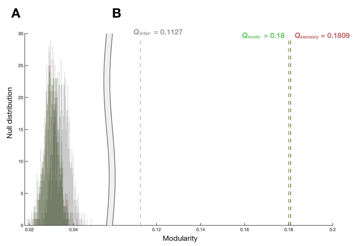
Figure S8: Testing of clustering assignments when the focus is on sensory neurons (red), interneurons (grey) or motoneurons (green). For each case, all nodes of other types are considered as one additional cluster. The null distributions of the modularity of random assignments to clusters are given on the left side of the plot (A).The dashed straight lines on the right represent values of modularity $Q$ for the clusters in Fig. S4 derived by the k-means approach (B). The x-axis is broken at $0.06$ for better visualization.

In Supplementary Fig. S8, we present the results of the statistical approach for the case of sensory (red plots), inter- (grey plots) and motoneurons (green plots). The modularity values for the assignments to clusters as found by k-means clustering (see Section 6.1) are marked with the dashed lines and labeled with $Q\textsubscript{sensory}$, $Q\textsubscript{inter-}$, and $Q\textsubscript{moto-}$ (Supplementary Fig. S8B). For the number of clusters estimated by the Silhouette method, we generated 999 random assignment vectors and calculated $Q$ each time, in order to build a null distribution (Supplementary Fig. S8A).

As $Q\textsubscript{sensory}$, $Q\textsubscript{inter-}$, and $Q\textsubscript{moto-}$ are above the corresponding distributions of modularity for random assignments, we conclude that the found clustering is significant. Since these modularity values are strictly greater than all other $Q$ values for random assignments, and, consequently, from any chosen percentile of the calculated distributions, the test rejects the null hypothesis that the chosen clustering is random at even very small significance levels. Finally, we note that the distribution of $Q$ in the case of interneurons is slightly closer to the corresponding value of $Q\textsubscript{inter-}$ than in the case of sensory or motoneurons. This can be expected, since interneurons are more strongly connected to other cell types, and thus, do not impose as strong communities as for the clusters formed from sensory or motoneurons.

6.3 Supplementary Figures

Figure S1: For energy concentration (A) and modified embedded distance (B) criteria, eigenspectra at bandwidth $W=100,150,200,279$, as depicted by increasingly darker blue or purple shades, respectively. Yellow and orange vertical bars map locations of the eigenspectra at which Slepian vectors are shown (C and D). They are displayed for increasing bandwidth going from left ($W=100$) to right ($W=279$, full bandwidth). For energy concentration (C), the first row illustrates two Slepian vectors mapping the start of the spectrum (normalized indices of $0.1$ — strongly concentrated in $\mathcal{S}$ — and $0.4$ — still concentrated, but less for lower bandwidth). The second row denotes two Slepian vectors from the second half of the spectrum (normalized indices of $0.6$ — mildly concentrated in $\mathcal{S}$ using a smaller bandwidth — and $0.9$ — not concentrated at all). Visualizations are similar for modified embedded distance (D), but in this case, low eigenvalues imply either non-concentrated (e.g., X axis, first row of plots) or mildly concentrated but low localized spatial frequency Slepian vectors (for instance, Y axis, first row of plots, $W=200$), while high eigenvalues relate to high localized spatial frequency Slepian vectors (see Y axis, second row of plots). See Van De Ville . (20171) for another preliminary analysis of the dataset from the modified embedded distance viewpoint. $\mu$ and $\xi$ values of the shown Slepian vectors are provided in parentheses on each axis.

Figure S2: Eigenspectrum of the newly developped $\zeta$ criterion (A), with vertical bars highlighting the locations of the spectrum at which four pairs of Slepian vectors were sampled for display (B, from first to fourth row as respectively depicted by yellow, orange, brown and red color codes). Results obtained with linear, quadratic and order 10 approximations, as well as from a full computation of $\mathbf{M}-\mathbf{L}^{1/2}\mathbf{M}\mathbf{L}^{1/2}$, are respectively shown from left to right. $\zeta$ values of the shown Slepian vectors are provided in parentheses on each axis.

Figure S3: Start (left column), intermediate (middle column) and end (right column) representations of sensory neuron (A), interneuron (B) or motoneuron (C) trajectories, respectively, setting cooperation weights for other neuron types to $1$, $0.5$ or $0$. Cells are labeled according to Varshney . (2011). The start representation is the same across cases, since then $\mathbf{M}=\mathbf{I}$ and the problem boils down to the eigendecomposition of the adjacency matrix $\mathbf{A}$, or equivalently of the Laplacian $\mathbf{L}=\mathbf{I}-\mathbf{A}$ highlighted in Fig. 1.

Figure S5: Focussing on (A) sensory neurons (red), (B) interneurons (black) or (C) motoneurons (green), two-dimensional visualization using alternative sets of Slepian vectors: first and second (first row), fourth and fifth (second row), or last two (third row). Cells are labeled according to Varshney . (2011). $\zeta$ values of the shown Slepian vectors are provided in parentheses on each axis.

Figure S6: Separate two-dimensional visualizations when only considering chemical synapses (left column) or gap junctions (right column) for sensory neurons (A), interneurons (B) or motoneurons (C). Cells are labeled according to Varshney . (2011). $\zeta$ values of the shown Slepian vectors are provided in parentheses on each axis.

Figure S7: Two-dimensional visualizations for sensory neurons (A), interneurons (B) or motoneurons (C) when representing each neuron as a function of its position along the X direction. A value of 0 indicates the location of the nerve ring, and positional data was retrieved from Varier  Kaiser (2011). $\zeta$ values of the shown Slepian vectors are provided in parentheses on each axis.

References

- Agaskar \BBA Lu (\APACyear2013) \APACinsertmetastarAgaskar.2013{APACrefauthors}Agaskar, A.\BCBT \BBA Lu, Y\BPBIM. \APACrefYearMonthDay2013. \BBOQ\APACrefatitleA Spectral Graph Uncertainty Principle A spectral graph uncertainty principle.\BBCQ \APACjournalVolNumPagesIEEE Transactions on Information Theory5974338–4356. \PrintBackRefs\CurrentBib
- Arenas \BOthers. (\APACyear2008) \APACinsertmetastarArenas.2008{APACrefauthors}Arenas, A., Fernández, A.\BCBL \BBA Gómez, S. \APACrefYearMonthDay2008\APACmonth05. \BBOQ\APACrefatitleAnalysis of the structure of complex networks at different resolution levels Analysis of the structure of complex networks at different resolution levels.\BBCQ \APACjournalVolNumPagesNew Journal of Physics105053039. \PrintBackRefs\CurrentBib
- Bargmann \BOthers. (\APACyear1993) \APACinsertmetastarBargmann1993{APACrefauthors}Bargmann, C\BPBII., Hartwieg, E.\BCBL \BBA Horvitz, H\BPBIR. \APACrefYearMonthDay1993. \BBOQ\APACrefatitleOdorant-selective genes and neurons mediate olfaction in C. elegans Odorant-selective genes and neurons mediate olfaction in C. elegans.\BBCQ \APACjournalVolNumPagesCell743515–527. \PrintBackRefs\CurrentBib
- Bargmann \BBA Horvitz (\APACyear1991) \APACinsertmetastarBargmann1991{APACrefauthors}Bargmann, C\BPBII.\BCBT \BBA Horvitz, H\BPBIR. \APACrefYearMonthDay1991. \BBOQ\APACrefatitleChemosensory neurons with overlapping functions direct chemotaxis to multiple chemicals in C. elegans Chemosensory neurons with overlapping functions direct chemotaxis to multiple chemicals in C. elegans.\BBCQ \APACjournalVolNumPagesNeuron75729–742. \PrintBackRefs\CurrentBib
- Barrios \BOthers. (\APACyear2012) \APACinsertmetastarBarrios2012{APACrefauthors}Barrios, A., Ghosh, R., Fang, C., Emmons, S\BPBIW.\BCBL \BBA Barr, M\BPBIM. \APACrefYearMonthDay2012. \BBOQ\APACrefatitlePDF-1 neuropeptide signaling modulates a neural circuit for mate-searching behavior in C. elegans PDF-1 neuropeptide signaling modulates a neural circuit for mate-searching behavior in C. elegans.\BBCQ \APACjournalVolNumPagesNature neuroscience15121675. \PrintBackRefs\CurrentBib
- Belkin \BBA Niyogi (\APACyear2003) \APACinsertmetastarBelkin.2003{APACrefauthors}Belkin, M.\BCBT \BBA Niyogi, P. \APACrefYearMonthDay2003. \BBOQ\APACrefatitleLaplacian eigenmaps for dimensionality reduction and data representation Laplacian eigenmaps for dimensionality reduction and data representation.\BBCQ \APACjournalVolNumPagesNeural Computation1561373–1396. \PrintBackRefs\CurrentBib
- Chalfie \BOthers. (\APACyear1985) \APACinsertmetastarChalfie1985{APACrefauthors}Chalfie, M., Sulston, J\BPBIE., White, J\BPBIG., Southgate, E., Thomson, J\BPBIN.\BCBL \BBA Brenner, S. \APACrefYearMonthDay1985. \BBOQ\APACrefatitleThe neural circuit for touch sensitivity in Caenorhabditis elegans The neural circuit for touch sensitivity in Caenorhabditis elegans.\BBCQ \APACjournalVolNumPagesJournal of Neuroscience54956–964. \PrintBackRefs\CurrentBib
- Chen \BOthers. (\APACyear2006) \APACinsertmetastarChen.2006{APACrefauthors}Chen, B\BPBIL., Hall, D\BPBIH.\BCBL \BBA Chklovskii, D\BPBIB. \APACrefYearMonthDay2006\APACmonth03. \BBOQ\APACrefatitleWiring optimization can relate neuronal structure and function Wiring optimization can relate neuronal structure and function.\BBCQ \APACjournalVolNumPagesProceedings of the National Academy of Sciences of the United States of America103124723–4728. \PrintBackRefs\CurrentBib
- Chung (\APACyear1997) \APACinsertmetastarChung.1997{APACrefauthors}Chung, F\BPBIR\BPBIK. \APACrefYear1997. \APACrefbtitleSpectral Graph Theory Spectral graph theory. \APACaddressPublisherProvidenceAmer. Math. Soc. \PrintBackRefs\CurrentBib
- Contreras \BOthers. (\APACyear2015) \APACinsertmetastarContreras2015{APACrefauthors}Contreras, J\BPBIA., Goñi, J., Risacher, S\BPBIL., Sporns, O.\BCBL \BBA Saykin, A\BPBIJ. \APACrefYearMonthDay2015oct. \BBOQ\APACrefatitleThe Structural and Functional Connectome and Prediction of Risk for Cognitive Impairment in Older Adults The structural and functional connectome and prediction of risk for cognitive impairment in older adults.\BBCQ \APACjournalVolNumPagesCurrent Behavioral Neuroscience Reports24234–245. {APACrefURL} https://doi.org/10.1007/s40473-015-0056-z {APACrefDOI} 10.1007/s40473-015-0056-z \PrintBackRefs\CurrentBib
- De Lange \BOthers. (\APACyear2014) \APACinsertmetastardeLange2014{APACrefauthors}De Lange, S., De Reus, M.\BCBL \BBA Van den Heuvel, M. \APACrefYearMonthDay2014. \BBOQ\APACrefatitleThe Laplacian spectrum of neural networks The laplacian spectrum of neural networks.\BBCQ \APACjournalVolNumPagesFrontiers in Computational Neuroscience71891–12. \PrintBackRefs\CurrentBib
- Fiedler (\APACyear1989) \APACinsertmetastarFiedler.1989{APACrefauthors}Fiedler, M. \APACrefYearMonthDay1989. \BBOQ\APACrefatitleLaplacian of graphs and algebraic connectivity Laplacian of graphs and algebraic connectivity.\BBCQ \APACjournalVolNumPagesCombinatorics and Graph Theory2557-70. \PrintBackRefs\CurrentBib
- Gray \BOthers. (\APACyear2005) \APACinsertmetastarGray2005{APACrefauthors}Gray, J\BPBIM., Hill, J\BPBIJ.\BCBL \BBA Bargmann, C\BPBII. \APACrefYearMonthDay2005. \BBOQ\APACrefatitleA circuit for navigation in Caenorhabditis elegans A circuit for navigation in Caenorhabditis elegans.\BBCQ \APACjournalVolNumPagesProceedings of the National Academy of Sciences10293184–3191. \PrintBackRefs\CurrentBib
- Hammond \BOthers. (\APACyear2011) \APACinsertmetastarHammond.2011{APACrefauthors}Hammond, D\BPBIK., Vandergheynst, P.\BCBL \BBA Gribonval, R. \APACrefYearMonthDay2011. \BBOQ\APACrefatitleWavelets on graphs via spectral graph theory Wavelets on graphs via spectral graph theory.\BBCQ \APACjournalVolNumPagesAppl. and Comp. Harm. Anal.302129–150. \PrintBackRefs\CurrentBib
- Hart \BOthers. (\APACyear1995) \APACinsertmetastarHart1995{APACrefauthors}Hart, A\BPBIC., Sims, S.\BCBL \BBA Kaplan, J\BPBIM. \APACrefYearMonthDay1995. \BBOQ\APACrefatitleSynaptic code for sensory modalities revealed by C. elegans GLR-1 glutamate receptor Synaptic code for sensory modalities revealed by C. elegans GLR-1 glutamate receptor.\BBCQ \APACjournalVolNumPagesNature378655282. \PrintBackRefs\CurrentBib
- Haspel \BOthers. (\APACyear2010) \APACinsertmetastarHaspel2010{APACrefauthors}Haspel, G., O’Donovan, M\BPBIJ.\BCBL \BBA Hart, A\BPBIC. \APACrefYearMonthDay2010. \BBOQ\APACrefatitleMotoneurons dedicated to either forward or backward locomotion in the nematode Caenorhabditis elegans Motoneurons dedicated to either forward or backward locomotion in the nematode Caenorhabditis elegans.\BBCQ \APACjournalVolNumPagesJournal of Neuroscience303311151–11156. \PrintBackRefs\CurrentBib
- Hobert (\APACyear2003) \APACinsertmetastarHobert2003{APACrefauthors}Hobert, O. \APACrefYearMonthDay2003. \BBOQ\APACrefatitleBehavioral plasticity in C. elegans: paradigms, circuits, genes Behavioral plasticity in C. elegans: paradigms, circuits, genes.\BBCQ \APACjournalVolNumPagesJournal of neurobiology541203–223. \PrintBackRefs\CurrentBib
- Hobert \BOthers. (\APACyear2002) \APACinsertmetastarHobert2002{APACrefauthors}Hobert, O., Johnston Jr, R\BPBIJ.\BCBL \BBA Chang, S. \APACrefYearMonthDay2002. \BBOQ\APACrefatitleLeft–right asymmetry in the nervous system: the Caenorhabditis elegans model Left–right asymmetry in the nervous system: the Caenorhabditis elegans model.\BBCQ \APACjournalVolNumPagesNature Reviews Neuroscience38629. \PrintBackRefs\CurrentBib
- Huang \BOthers. (\APACyear2018) \APACinsertmetastarHuang_2018{APACrefauthors}Huang, W., Bolton, T\BPBIA., Medaglia, J\BPBID., Bassett, D\BPBIS., Ribeiro, A.\BCBL \BBA Van De Ville, D. \APACrefYearMonthDay2018. \BBOQ\APACrefatitleA Graph Signal Processing Perspective on Functional Brain Imaging A graph signal processing perspective on functional brain imaging.\BBCQ \APACjournalVolNumPagesProceedings of the IEEE. \PrintBackRefs\CurrentBib
- Irion \BBA Saito (\APACyear2014) \APACinsertmetastarIrion.2014{APACrefauthors}Irion, J.\BCBT \BBA Saito, N. \APACrefYearMonthDay2014. \BBOQ\APACrefatitleHierarchical graph Laplacian eigen transforms Hierarchical graph Laplacian eigen transforms.\BBCQ \APACjournalVolNumPagesJSIAM Letters621-24. {APACrefDOI} 10.14495/jsiaml.6.21 \PrintBackRefs\CurrentBib
- Kawano \BOthers. (\APACyear2011) \APACinsertmetastarKawano2011{APACrefauthors}Kawano, T., Po, M\BPBID., Gao, S., Leung, G., Ryu, W\BPBIS.\BCBL \BBA Zhen, M. \APACrefYearMonthDay2011. \BBOQ\APACrefatitleAn imbalancing act: gap junctions reduce the backward motor circuit activity to bias C. elegans for forward locomotion An imbalancing act: gap junctions reduce the backward motor circuit activity to bias C. elegans for forward locomotion.\BBCQ \APACjournalVolNumPagesNeuron724572–586. \PrintBackRefs\CurrentBib
- Krasuski \BOthers. (\APACyear1998) \APACinsertmetastarKrasuski1998{APACrefauthors}Krasuski, J\BPBIS., Alexander, G\BPBIE., Horwitz, B., Daly, E\BPBIM., Murphy, D\BPBIG., Rapoport, S\BPBII.\BCBL \BBA Schapiro, M\BPBIB. \APACrefYearMonthDay1998jan. \BBOQ\APACrefatitleVolumes of Medial Temporal Lobe Structures in Patients with Alzheimer’s Disease and Mild Cognitive Impairment (and in Healthy Controls) Volumes of medial temporal lobe structures in patients with alzheimer’s disease and mild cognitive impairment (and in healthy controls).\BBCQ \APACjournalVolNumPagesBiological Psychiatry43160–68. {APACrefURL} https://doi.org/10.1016/s0006-3223(97)00013-9 {APACrefDOI} 10.1016/s0006-3223(97)00013-9 \PrintBackRefs\CurrentBib
- Lehoucq \BBA Sorensen (\APACyear1996) \APACinsertmetastarLehoucq.1996{APACrefauthors}Lehoucq, R\BPBIB.\BCBT \BBA Sorensen, D\BPBIC. \APACrefYearMonthDay1996. \BBOQ\APACrefatitleDeflation techniques for an implicitly restarted Arnoldi iteration Deflation techniques for an implicitly restarted Arnoldi iteration.\BBCQ \APACjournalVolNumPagesSIAM Journal on Matrix Analysis and Applications174789–821. \PrintBackRefs\CurrentBib
- Li \BOthers. (\APACyear2012) \APACinsertmetastarLi2012{APACrefauthors}Li, Z., Li, Y., Yi, Y., Huang, W., Yang, S., Niu, W.\BDBLothers \APACrefYearMonthDay2012. \BBOQ\APACrefatitleDissecting a central flip-flop circuit that integrates contradictory sensory cues in C. elegans feeding regulation Dissecting a central flip-flop circuit that integrates contradictory sensory cues in C. elegans feeding regulation.\BBCQ \APACjournalVolNumPagesNature communications3776. \PrintBackRefs\CurrentBib
- Lu \BBA Pearce (\APACyear2000) \APACinsertmetastarLu2000eigvalbounds{APACrefauthors}Lu, L\BHBIZ.\BCBT \BBA Pearce, C\BPBIE\BPBIM. \APACrefYearMonthDay2000. \BBOQ\APACrefatitleSome new bounds for singular values and eigenvalues of matrix products Some new bounds for singular values and eigenvalues of matrix products.\BBCQ \APACjournalVolNumPagesAnnals of Operations Research981-4141–148. \PrintBackRefs\CurrentBib
- Luo \BOthers. (\APACyear2014) \APACinsertmetastarLuo2014{APACrefauthors}Luo, L., Wen, Q., Ren, J., Hendricks, M., Gershow, M., Qin, Y.\BDBLothers \APACrefYearMonthDay2014. \BBOQ\APACrefatitleDynamic encoding of perception, memory, and movement in a C. elegans chemotaxis circuit Dynamic encoding of perception, memory, and movement in a C. elegans chemotaxis circuit.\BBCQ \APACjournalVolNumPagesNeuron8251115–1128. \PrintBackRefs\CurrentBib
- Mahadevan \BBA Maggioni (\APACyear2006) \APACinsertmetastarMahadevan.2006{APACrefauthors}Mahadevan, S.\BCBT \BBA Maggioni, M. \APACrefYearMonthDay2006. \BBOQ\APACrefatitleValue Function Approximation with Diffusion Wavelets and Laplacian Eigenfunctions Value function approximation with diffusion wavelets and Laplacian eigenfunctions.\BBCQ \BIn Y. Weiss, B. Schölkopf\BCBL \BBA J\BPBIC. Platt (\BEDS), \APACrefbtitleAdvances in Neural Information Processing Systems 18 Advances in neural information processing systems 18 (\BPGS 843–850). \APACaddressPublisherMIT Press. \PrintBackRefs\CurrentBib
- Mhaskar (\APACyear2018) \APACinsertmetastarMhaskar.2018{APACrefauthors}Mhaskar, H. \APACrefYearMonthDay2018may. \BBOQ\APACrefatitleA unified framework for harmonic analysis of functions on directed graphs and changing data A unified framework for harmonic analysis of functions on directed graphs and changing data.\BBCQ \APACjournalVolNumPagesApplied and Computational Harmonic Analysis443611–644. {APACrefURL} https://doi.org/10.1016/j.acha.2016.06.007 {APACrefDOI} 10.1016/j.acha.2016.06.007 \PrintBackRefs\CurrentBib
- Mori \BBA Ohshima (\APACyear1995) \APACinsertmetastarMori1995{APACrefauthors}Mori, I.\BCBT \BBA Ohshima, Y. \APACrefYearMonthDay1995. \BBOQ\APACrefatitleNeural regulation of thermotaxis in Caenorhabditis elegans Neural regulation of thermotaxis in Caenorhabditis elegans.\BBCQ \APACjournalVolNumPagesNature3766538344. \PrintBackRefs\CurrentBib
- M. Newman (\APACyear2010) \APACinsertmetastarNewman.2010{APACrefauthors}Newman, M. \APACrefYear2010. \APACrefbtitleNetworks: An Introduction Networks: An introduction. \APACaddressPublisherNew York, NY, USAOxford Univ. Press. \PrintBackRefs\CurrentBib
- M\BPBIE\BPBIJ. Newman (\APACyear2006) \APACinsertmetastarnewman2006{APACrefauthors}Newman, M\BPBIE\BPBIJ. \APACrefYearMonthDay2006sep. \BBOQ\APACrefatitleFinding community structure in networks using the eigenvectors of matrices Finding community structure in networks using the eigenvectors of matrices.\BBCQ \APACjournalVolNumPagesPhysical Review E743. {APACrefURL} https://doi.org/10.1103/physreve.74.036104 {APACrefDOI} 10.1103/physreve.74.036104 \PrintBackRefs\CurrentBib
- Ortega \BOthers. (\APACyear2018) \APACinsertmetastarOrtega2018{APACrefauthors}Ortega, A., Frossard, P., Kovačević, J., Moura, J\BPBIM.\BCBL \BBA Vandergheynst, P. \APACrefYearMonthDay2018. \BBOQ\APACrefatitleGraph signal processing: Overview, challenges, and applications Graph signal processing: Overview, challenges, and applications.\BBCQ \APACjournalVolNumPagesProceedings of the IEEE1065808–828. \PrintBackRefs\CurrentBib
- Pirondini \BOthers. (\APACyear2016) \APACinsertmetastarpirondini1601{APACrefauthors}Pirondini, E., Vybornova, A., Coscia, M.\BCBL \BBA Van De Ville, D. \APACrefYearMonthDay2016September. \BBOQ\APACrefatitleSpectral Method for Generating Surrogate Graph Signals Spectral method for generating surrogate graph signals.\BBCQ \APACjournalVolNumPagesIEEE Signal Processing Letters2391275-1278. {APACrefURL} /index.php/software/graph-surrogates {APACrefDOI} 10.1109/LSP.2016.2594072 \PrintBackRefs\CurrentBib
- Rousseeuw (\APACyear1987) \APACinsertmetastarRousseeuw1987{APACrefauthors}Rousseeuw, P\BPBIJ. \APACrefYearMonthDay1987nov. \BBOQ\APACrefatitleSilhouettes: A graphical aid to the interpretation and validation of cluster analysis Silhouettes: A graphical aid to the interpretation and validation of cluster analysis.\BBCQ \APACjournalVolNumPagesJournal of Computational and Applied Mathematics2053–65. {APACrefURL} https://doi.org/10.1016/0377-0427(87)90125-7 {APACrefDOI} 10.1016/0377-0427(87)90125-7 \PrintBackRefs\CurrentBib
- Roweis (\APACyear2000) \APACinsertmetastarRoweis2000{APACrefauthors}Roweis, S\BPBIT. \APACrefYearMonthDay2000dec. \BBOQ\APACrefatitleNonlinear Dimensionality Reduction by Locally Linear Embedding Nonlinear dimensionality reduction by locally linear embedding.\BBCQ \APACjournalVolNumPagesScience29055002323–2326. {APACrefURL} https://doi.org/10.1126/science.290.5500.2323 {APACrefDOI} 10.1126/science.290.5500.2323 \PrintBackRefs\CurrentBib
- Sammon (\APACyear1969) \APACinsertmetastarSammon1969{APACrefauthors}Sammon, J. \APACrefYearMonthDay1969may. \BBOQ\APACrefatitleA Nonlinear Mapping for Data Structure Analysis A nonlinear mapping for data structure analysis.\BBCQ \APACjournalVolNumPagesIEEE Transactions on ComputersC-185401–409. {APACrefURL} https://doi.org/10.1109/t-c.1969.222678 {APACrefDOI} 10.1109/t-c.1969.222678 \PrintBackRefs\CurrentBib
- Sandryhaila \BBA Moura (\APACyear2013) \APACinsertmetastarSandryhaila.2013{APACrefauthors}Sandryhaila, A.\BCBT \BBA Moura, J\BPBIM\BPBIF. \APACrefYearMonthDay2013\APACmonth03. \BBOQ\APACrefatitleDiscrete Signal Processing on Graphs Discrete signal processing on graphs.\BBCQ \APACjournalVolNumPagesIEEE Transactions on Signal Processing6171644–1656. \PrintBackRefs\CurrentBib
- Sawin \BOthers. (\APACyear2000) \APACinsertmetastarSawin2000{APACrefauthors}Sawin, E\BPBIR., Ranganathan, R.\BCBL \BBA Horvitz, H\BPBIR. \APACrefYearMonthDay2000. \BBOQ\APACrefatitleC. elegans locomotory rate is modulated by the environment through a dopaminergic pathway and by experience through a serotonergic pathway C. elegans locomotory rate is modulated by the environment through a dopaminergic pathway and by experience through a serotonergic pathway.\BBCQ \APACjournalVolNumPagesNeuron263619–631. \PrintBackRefs\CurrentBib
- Schaub \BOthers. (\APACyear2018) \APACinsertmetastarSchaub2018{APACrefauthors}Schaub, M\BPBIT., Delvenne, J\BHBIC., Lambiotte, R.\BCBL \BBA Barahona, M. \APACrefYearMonthDay2018. \APACrefbtitleMultiscale dynamical embeddings of complex networks. Multiscale dynamical embeddings of complex networks. \PrintBackRefs\CurrentBib
- Schönemann (\APACyear1966) \APACinsertmetastarProcrustes{APACrefauthors}Schönemann, P\BPBIH. \APACrefYearMonthDay1966. \BBOQ\APACrefatitleA generalized solution of the orthogonal procrustes problem A generalized solution of the orthogonal procrustes problem.\BBCQ \APACjournalVolNumPagesPsychometrika3111–10. \PrintBackRefs\CurrentBib
- Schuske \BOthers. (\APACyear2004) \APACinsertmetastarSchuske2004{APACrefauthors}Schuske, K., Beg, A\BPBIA.\BCBL \BBA Jorgensen, E\BPBIM. \APACrefYearMonthDay2004. \BBOQ\APACrefatitleThe GABA nervous system in C. elegans The GABA nervous system in C. elegans.\BBCQ \APACjournalVolNumPagesTrends in neurosciences277407–414. \PrintBackRefs\CurrentBib
- Shen \BBA Meyer (\APACyear2008) \APACinsertmetastarShen2008{APACrefauthors}Shen, X.\BCBT \BBA Meyer, F\BPBIG. \APACrefYearMonthDay2008jul. \BBOQ\APACrefatitleLow-dimensional embedding of fMRI datasets Low-dimensional embedding of fMRI datasets.\BBCQ \APACjournalVolNumPagesNeuroImage413886–902. {APACrefURL} https://doi.org/10.1016/j.neuroimage.2008.02.051 {APACrefDOI} 10.1016/j.neuroimage.2008.02.051 \PrintBackRefs\CurrentBib
- Shuman \BOthers. (\APACyear2013) \APACinsertmetastarShuman.2013{APACrefauthors}Shuman, D\BPBII., Narang, S\BPBIK., Frossard, P., Ortega, A.\BCBL \BBA Vandergheynst, P. \APACrefYearMonthDay2013. \BBOQ\APACrefatitleThe emerging field of signal processing on graphs: Extending high-dimensional data analysis to networks and other irregular domains The emerging field of signal processing on graphs: Extending high-dimensional data analysis to networks and other irregular domains.\BBCQ \APACjournalVolNumPagesIEEE Signal Processing Magazine30383–98. \PrintBackRefs\CurrentBib
- Slepian (\APACyear1978) \APACinsertmetastarSlepian.1978{APACrefauthors}Slepian, D. \APACrefYearMonthDay1978. \BBOQ\APACrefatitleProlate Spheroidal Wave-Functions, Fourier-Analysis, and Uncertainty. Discrete Case Prolate spheroidal wave-functions, Fourier-analysis, and uncertainty. Discrete case.\BBCQ \APACjournalVolNumPagesBell System Technical Journal5751371–1430. \PrintBackRefs\CurrentBib
- Slepian \BBA Pollak (\APACyear1961) \APACinsertmetastarSlepian.1961{APACrefauthors}Slepian, D.\BCBT \BBA Pollak, H\BPBIO. \APACrefYearMonthDay1961. \BBOQ\APACrefatitleProlate Spheroidal Wave Functions, Fourier Analysis and Uncertainty Prolate spheroidal wave functions, Fourier analysis and uncertainty.\BBCQ \APACjournalVolNumPagesBell System Technical Journal40143–63. \PrintBackRefs\CurrentBib
- Teke \BBA Vaidyanathan (\APACyear\BIP) \APACinsertmetastarTeke.2017{APACrefauthors}Teke, O.\BCBT \BBA Vaidyanathan, P\BPBIP. \APACrefYearMonthDay\BIP. \BBOQ\APACrefatitleUncertainty Principles and Sparse Eigenvectors of Graphs Uncertainty principles and sparse eigenvectors of graphs.\BBCQ \APACjournalVolNumPagesIEEE Transactions on Signal Processing. \PrintBackRefs\CurrentBib
- Tenenbaum (\APACyear2000) \APACinsertmetastarTenenbaum2000{APACrefauthors}Tenenbaum, J\BPBIB. \APACrefYearMonthDay2000dec. \BBOQ\APACrefatitleA Global Geometric Framework for Nonlinear Dimensionality Reduction A global geometric framework for nonlinear dimensionality reduction.\BBCQ \APACjournalVolNumPagesScience29055002319–2323. {APACrefURL} https://doi.org/10.1126/science.290.5500.2319 {APACrefDOI} 10.1126/science.290.5500.2319 \PrintBackRefs\CurrentBib
- Tsitsvero \BOthers. (\APACyear2016) \APACinsertmetastarTsitsvero.2016{APACrefauthors}Tsitsvero, M., Barbarossa, S.\BCBL \BBA Di Lorenzo, P. \APACrefYearMonthDay2016. \BBOQ\APACrefatitleSignals on Graphs: Uncertainty Principle and Sampling Signals on graphs: Uncertainty principle and sampling.\BBCQ \APACjournalVolNumPagesIEEE Transactions on Signal Processing64184845–4860. \PrintBackRefs\CurrentBib
- van den Heuvel \BBA Sporns (\APACyear2013) \APACinsertmetastarvandenHeuvel2013{APACrefauthors}van den Heuvel, M\BPBIP.\BCBT \BBA Sporns, O. \APACrefYearMonthDay2013dec. \BBOQ\APACrefatitleNetwork hubs in the human brain Network hubs in the human brain.\BBCQ \APACjournalVolNumPagesTrends in Cognitive Sciences1712683–696. {APACrefURL} https://doi.org/10.1016/j.tics.2013.09.012 {APACrefDOI} 10.1016/j.tics.2013.09.012 \PrintBackRefs\CurrentBib
- van der Maaten \BBA Hinton (\APACyear2008) \APACinsertmetastarvanDerMaaten2008{APACrefauthors}van der Maaten, L.\BCBT \BBA Hinton, G. \APACrefYearMonthDay2008. \BBOQ\APACrefatitleVisualizing Data using t-SNE Visualizing data using t-SNE.\BBCQ \APACjournalVolNumPagesJournal of Machine Learning Research92579–2605. {APACrefURL} http://www.jmlr.org/papers/v9/vandermaaten08a.html \PrintBackRefs\CurrentBib
- Van De Ville (\APACyear2016) \APACinsertmetastarVDV_Slepians_1{APACrefauthors}Van De Ville, D. \APACrefYearMonthDay2016. \BBOQ\APACrefatitleSteering Macro-Scale Network Community Structure by Micro-Scale Features Steering macro-scale network community structure by micro-scale features.\BBCQ \APACjournalVolNumPagesarXiv preprint arXiv:1603.05623. \PrintBackRefs\CurrentBib
- Van De Ville \BOthers. (\APACyear2017\APACexlab\BCnt1) \APACinsertmetastarVDV2017_Guiding{APACrefauthors}Van De Ville, D., Demesmaeker, R.\BCBL \BBA Preti, M\BPBIG. \APACrefYearMonthDay2017\BCnt1. \BBOQ\APACrefatitleGuiding network analysis using graph slepians: an illustration for the C. Elegans connectome Guiding network analysis using graph slepians: an illustration for the c. elegans connectome.\BBCQ \BIn \APACrefbtitleWavelets and Sparsity XVII Wavelets and sparsity xvii (\BVOL 10394, \BPG 103941Y). \PrintBackRefs\CurrentBib
- Van De Ville \BOthers. (\APACyear2017\APACexlab\BCnt2) \APACinsertmetastarvandeville1701{APACrefauthors}Van De Ville, D., Demesmaeker, R.\BCBL \BBA Preti, M\BPBIG. \APACrefYearMonthDay2017\BCnt2. \BBOQ\APACrefatitleWhen Slepian Meets Fiedler: Putting a Focus on the Graph Spectrum When Slepian meets Fiedler: Putting a focus on the graph spectrum.\BBCQ \APACjournalVolNumPagesIEEE Signal Processing Letters241001–1004. {APACrefURL} /index.php/software/graph-slepians {APACrefDOI} 10.1109/LSP.2017.2704359 \PrintBackRefs\CurrentBib
- Varier \BBA Kaiser (\APACyear2011) \APACinsertmetastarVarier2011{APACrefauthors}Varier, S.\BCBT \BBA Kaiser, M. \APACrefYearMonthDay2011. \BBOQ\APACrefatitleNeural development features: Spatio-temporal development of the Caenorhabditis elegans neuronal network Neural development features: Spatio-temporal development of the Caenorhabditis elegans neuronal network.\BBCQ \APACjournalVolNumPagesPLoS computational biology71e1001044. \PrintBackRefs\CurrentBib
- Varshney \BOthers. (\APACyear2011) \APACinsertmetastarVarshney2011{APACrefauthors}Varshney, L\BPBIR., Chen, B\BPBIL., Paniagua, E., Hall, D\BPBIH.\BCBL \BBA Chklovskii, D\BPBIB. \APACrefYearMonthDay2011. \BBOQ\APACrefatitleStructural properties of the Caenorhabditis elegans neuronal network Structural properties of the caenorhabditis elegans neuronal network.\BBCQ \APACjournalVolNumPagesPLoS computational biology72e1001066. \PrintBackRefs\CurrentBib
- Von Luxburg (\APACyear2007) \APACinsertmetastarVonLuxburg2007{APACrefauthors}Von Luxburg, U. \APACrefYearMonthDay2007. \BBOQ\APACrefatitleA tutorial on spectral clustering A tutorial on spectral clustering.\BBCQ \APACjournalVolNumPagesStatistics and computing174395–416. \PrintBackRefs\CurrentBib
- Wakabayashi \BOthers. (\APACyear2004) \APACinsertmetastarWakabayashi2004{APACrefauthors}Wakabayashi, T., Kitagawa, I.\BCBL \BBA Shingai, R. \APACrefYearMonthDay2004. \BBOQ\APACrefatitleNeurons regulating the duration of forward locomotion in Caenorhabditis elegans Neurons regulating the duration of forward locomotion in Caenorhabditis elegans.\BBCQ \APACjournalVolNumPagesNeuroscience research501103–111. \PrintBackRefs\CurrentBib
- White \BOthers. (\APACyear1986) \APACinsertmetastarWhite1986{APACrefauthors}White, J\BPBIG., Southgate, E., Thomson, J\BPBIN.\BCBL \BBA Brenner, S. \APACrefYearMonthDay1986. \BBOQ\APACrefatitleThe structure of the nervous system of the nematode Caenorhabditis elegans The structure of the nervous system of the nematode Caenorhabditis elegans.\BBCQ \APACjournalVolNumPagesPhilos Trans R Soc Lond B Biol Sci31411651–340. \PrintBackRefs\CurrentBib
- Wicks \BBA Rankin (\APACyear1995) \APACinsertmetastarWicks1995{APACrefauthors}Wicks, S\BPBIR.\BCBT \BBA Rankin, C\BPBIH. \APACrefYearMonthDay1995. \BBOQ\APACrefatitleIntegration of mechanosensory stimuli in Caenorhabditis elegans Integration of mechanosensory stimuli in Caenorhabditis elegans.\BBCQ \APACjournalVolNumPagesJournal of Neuroscience1532434–2444. \PrintBackRefs\CurrentBib