Link between brightest cluster galaxy properties and large scale extensions of 38 DAFT/FADA and CLASH clusters in the redshift range $0.2<z<0.9$

Abstract

Context. In the context of large-scale structure formation, clusters of galaxies are located at the nodes of the cosmic web, and continue to accrete galaxies and groups along filaments. In some cases, they show a very large extension and a preferential direction. Brightest cluster galaxies (BCGs) are believed to grow through the accretion of many small galaxies, and their structural properties are therefore expected to vary with redshift. In some cases BCGs show an orientation comparable to that of the cluster to which they belong.

Aims. We analyse the morphological properties of 38 BCGs from the DAFT/FADA and CLASH surveys, and compare the position angles of their major axes to the direction of the cluster elongation at large scale (several Mpc).

Methods. The morphological properties of the BCGs were studied by applying the GALFIT software to HST images and fitting the light distribution with one or two Sérsic laws, or with a Nuker plus a Sérsic law. The cluster elongations at very large scale were estimated by computing density maps of red sequence galaxies.

Results. The morphological analysis of the 38 BCGs shows that in 11 cases a single Sérsic law is sufficient to account for the surface brightness, while for all the other clusters two Sérsic laws are necessary. In five cases, a Nuker plus a Sérsic law give a better fit. For the outer Sérsic component, the effective radius increases with decreasing redshift, and the effective surface brightness decreases with effective radius, following the Kormendy law. An agreement between the major axis of the BCG and the cluster elongation at large scale within $\pm 30$ deg is found for 12 clusters out of the 21 for which the PAs of the BCG and of the large-scale structure can be defined.

Conclusions. The variation with redshift of the effective radius of the outer Sérsic component agrees with the growing of BCGs by accretion of smaller galaxies from z=0.9 to 0.2, and it would be interesting to investigate this variation at higher redshift. The directions of the elongations of BCGs and of their host clusters and large scale structures surrounding them agree for 12 objects out of 21, implying that a larger sample is necessary to reach more definite conclusions.

1 Introduction

The brightest cluster galaxies (hereafter BCGs) are typically more than one magnitude brighter than the second brightest galaxy and have long been a topic of investigation, both based on observations and on numerical simulations to explain their formation (see e.g. Aragón-Salamanca et al., 1998). Their very high mass (typically $10^{13}$ M_⊙) and extended stellar envelope suggest that they have formed by the accretion of many galaxies (e.g. De Lucia & Blaizot 2007, Lavoie et al. 2016 and references therein). The alignments of the great axes of BCGs with the main directions of the clusters to which they belong has been observed in a number of occasions, suggesting that the accretion of smaller galaxies by the BCG occurs predominantly along the direction of the cluster elongation. This seems also to be the case for superclusters. For example, Jöeveer et al. (1978) showed that in the Perseus–Pisces supercluster the main galaxies of the clusters are directed along the chain connecting this supercluster to other nearby superclusters. They concluded that there must be a physical link between cluster galaxies and their environment, suggesting a common origin and evolution of galaxies and galaxy clusters in the cosmic web. Many studies later confirmed the presence of alignments of brightest cluster galaxies (and sometimes of several bright cluster galaxies, not just the brightest one) in all kinds of large scale structures (West & Blakeslee 2000, Plionis & Basilakos 2002, Hopkins et al. 2005, Paz et al. 2011, Tempel et al. 2015, Tempel & Tamm 2015, Foëx et al. 2017, Hirv et al. 2017, West et al. 2017, Einasto et al. 2018).

Large-scale elongations and neighbouring clusters have been observed around a number of clusters at various redshifts up to $z\leq 0.9$ based on density maps computed from catalogues of galaxies selected around the cluster red sequence (Durret et al. 2016 and references therein). In some cases, the extensions are much larger than the typical sizes of clusters, suggesting we are detecting matter that may be associated with the clusters and/or infalling into them, or in some cases pairs of clusters or even superclusters. In view of the alignments found between the BCGs and large scale structure mentioned above, we propose to extend the sample of studied BCGs, by analysing the properties of a sample of 38 BCGs covering the redshift range $0.2\leq z\leq 0.9$, based on high quality HST images in the F814W band. Our aims are: 1) to fit the BCGs with several models and see if some of their properties vary with redshift, 2) to compare the position angles of their major axes with the general elongation of the clusters derived from galaxy density maps of red sequence galaxies.

2 Sample and data

The sample of BCGs studied here includes 38 massive clusters. The masses of the CLASH clusters are in the range $5\ 10^{14}<M_{vir}<3\ 10^{15}$ M_⊙ (Postman et al. 2012) and those of the DAFT/FADA have masses ${\rm M_{200}}\geq 3\ 10^{14}$ M_⊙ (see e.g. Martinet et al. 2015).

The BCGs cover the redshift range $0.206\leq z\leq 0.890$ and have HST ACS imaging available in the F814W band (except for ZwCl13332 which was observed in the F775W band). Out of these, 21 clusters were taken from the DAFT/FADA survey (Guennou et al. 2010) and 17 from the Cluster Lensing And Supernova survey with Hubble (CLASH) survey (Postman et al. 2012). Four clusters are common to both surveys, in which case we used the CLASH data. We limited our sample to the clusters with good quality data in the BCG area, and eliminated those where a bright star or galaxy was located too close to the BCG on the image.

For the DAFT/FADA clusters, the data were reduced with a modified version of the HAGGLeS pipeline (Bradac et al. 2008) to subtract the background and eliminate the bad pixels, and with Multidrizzle (Koekemoer et al. 2011) to combine all the images for each cluster and obtain a final image with a pixel size of 50 mas. For the CLASH clusters, the reduction was made by the CLASH team using MosaicDrizzle (Koekemoer et al. 2011), leading to images with a pixel size of 30 mas. Since we are mostly interested here by the properties of the BCGs at large scales, the fact that our images are sampled with two different pixel sizes is not a problem.

Table 1: Sample of 38 clusters in which the BCG was studied in detail and in a subsample of which the large scale structure around the cluster was explored with a density map. The columns are : full cluster name, coordinates of the BCG, redshift, scale, relevant survey(s), and for the density maps: instrument (M=CFHT/MegaCam, S=Subaru/SuprimeCam, V=ESO VLT/FORS2), filters. The coordinates of BMW-HRI J122657.3+333253 are wrong in NED and have been corrected here. LCDCS 0829 is often also found under the name RX J1347.5-1145.

Cluster	RA (J2000.0)	DEC (J2000.0)	Redshift	scale	Survey	Instrument	Filters
				(kpc/”)
Cl0016+1609	$00:18:33.80$	$+16:26:17.0$	$0.5455$	6.385	CLASH, DAFT/FADA	M	g’,i’
Abell 209	$01:31:52.55$	$-13:36:40.5$	$0.206$	3.377	CLASH	S	B,R
Cl J0152.7-1357	$01:52:41.00$	$-13:57:45.0$	$0.8310$	7.603	DAFT/FADA	S	V,R
MACS J0329.6-0211	$03:29:41.50$	$-02:11:46.0$	$0.450$	5.759	CLASH	S	B,I
MACS J0416.1-2403	$04:16:09.13$	$-24:04:03.5$	$0.396$	5.340	CLASH	S	B,I
MACS J0429.6-0253	$04:29:36.00$	$-02:53:08.0$	$0.399$	5.365	CLASH	S	V,I
MACS J0454.1-0300	$04:54:11.10$	$-03:00:54.0$	$0.5377$	6.339	DAFT/FADA	M	g’,z’
MACS J0647.7+7015	$06:47:50.50$	$+70:14:55.0$	$0.584$	6.130	CLASH, DAFT/FADA	S	V,I
MACS J0717.5+3745	$07:17:32.52$	$+37:44:34.9$	$0.548$	6.400	CLASH	S	V,I
MACS J0744.9+3927	$07:44:52.80$	$+39:27:26.6$	$0.686$	7.087	CLASH	S	V,I
Abell 611	$08:00:56.82$	$+36:03:23.6$	$0.288$	4.329	CLASH	S	B,R
Abell 851	$09:42:58.00$	$+46:59:12.0$	$0.4069$	5.429	DAFT/FADA	M	g’,i’
LCDCS 0110	$10:37:52.36$	$-12:44:49.0$	$0.5789$	6.574	DAFT/FADA
LCDCS 0130	$10:40:40.27$	$-11:56:04.2$	$0.7043$	7.163	DAFT/FADA
LCDCS 0172	$10:54:24.42$	$-11:46:19.4$	$0.6972$	7.134	DAFT/FADA	V	V,I
LCDCS 0173	$10:54:43.53$	$-12:45:51.9$	$0.7498$	7.337	DAFT/FADA
CL J1103.7-1245	$11:03:34.95$	$-12:46:46.4$	$0.6300$	6.835	DAFT/FADA
MACS J1115.8+0129	$11:15:51.91$	$+01:29:55.0$	$0.352$	4.958	CLASH	S	B,R
LCDCS 0340	$11:38:10.18$	$-11:33:38.1$	$0.4798$	5.969	DAFT/FADA
MACS J1149.6+2223	$11:49:35.71$	$+22:23:54.8$	$0.544$	6.376	CLASH	S	B,R
MACS J1206.2-0847	$12:06:12.15$	$-08:48:03.4$	$0.440$	5.685	CLASH	M	r’,z’
LCDCS 0504	$12:16:45.23$	$-12:01:17.4$	$0.7943$	7.490	DAFT/FADA
BMW-HRI J122657.3+333253	$12:26:58.25$	$+33:32:48.6$	$0.8900$	7.765	CLASH, DAFT/FADA	S	V,I
LCDCS 0531	$12:27:58.91$	$-11:35:13.8$	$0.6355$	6.861	DAFT/FADA
LCDCS 0541	$12:32:30.29$	$-12:50:36.5$	$0.5414$	6.361	DAFT/FADA
MACS J1311-0310	$13:11:01.80$	$-03:10:39.7$	$0.494$	6.065	CLASH	S	B,R
ZwCl 1332.8+5043	$13:34:20.40$	$+50:31:05.0$	$0.6200$	6.786	DAFT/FADA	M	g’,r’
LCDCS 0829	$13:47:30.60$	$-11:45:10.0$	$0.4510$	5.767	CLASH	S	B,R
LCDCS 0853	$13:54:09.75$	$-12:31:01.4$	$0.7627$	7.383	DAFT/FADA
MACS J1621.4+3810	$16:21:24.70$	$+38:10:08.0$	$0.4650$	5.867	DAFT/FADA	S	V,I
OC02 J1701+6412	$17:01:23.00$	$+64:14:09.0$	$0.4530$	5.781	DAFT/FADA	M	g’,i’
MACS J1720.2+3536	$17:20:16.75$	$+35:36:26.2$	$0.391$	5.298	CLASH	S	B,I
ABELL 2261	$17:22:27.10$	$+32:08:02.0$	$0.2240$	3.601	CLASH	S	B,R
MACS J2129.4-0741	$21:29:26.20$	$-07:41:26.0$	$0.5889$	6.627	CLASH, DAFT/FADA	S	V,I
RX J2129+0005	$21:29:39.96$	$+00:05:21.2$	$0.234$	3.722	CLASH	S	B,R
MS 2137.3-2353	$21:40:15.16$	$-23:39:40.1$	$0.313$	4.586	CLASH	S	B,R
RX J2248-4431	$22:48:43.97$	$-44:31:51.3$	$0.348$	4.921	CLASH
RX J2328.8+1453	$23:28:49.90$	$+14:53:12.0$	$0.4970$	6.084	DAFT/FADA	M	g’,i’

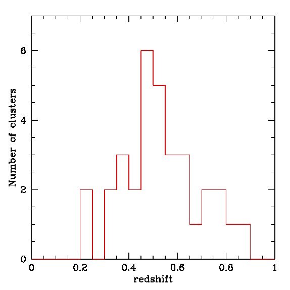
Figure 1: Histogram of the redshifts for the 38 BCGs of the sample.

The list of the 38 clusters analysed here is given in Table 1. We give the full names of all the clusters in column 1, but use abridged names in the text to make them more readable. The coordinates given in Table 1 are those of the BCG, which in a few cases differ slightly from those given in NED for the cluster. The scales given in column 5 were computed with Ned Wright’s cosmology calculator, taking H${}_{0}=70$ km s^-1 Mpc^-1, $\Omega_{\rm M}=0.3$ and $\Omega_{\rm vac}=0.7$. A histogram of the redshifts of the 38 BCGs of our sample is shown in Fig. 1.

3 Surface brightness analysis of BCGs

3.1 The method

To fit the surface brightnesses of BCGs, we used the GALFIT software developed by Peng et al. (2002). Before running GALFIT, the knowledge of several parameters is required. First, the PSF must be defined. This was done for all the CLASH clusters by Martinet et al. (2017), who measured the FWHM of stars on each of the images in the F814W band (using the PSFEx software developed by E. Bertin and found values between 0.05 and 0.25 arcsec (see Martinet et al. 2017, Table 1). The properties of the HST ACS instrument in the F814W filter leads to observe 80% of the energy received in a radius of $\sim 0.2$ arcsec and 90% in a radius of $\sim 0.5$ arcsec. The values of the effective radius of the inner component $R_{e,int}$ that we find (see below) are in the range 0.69 to 14.94 kpc, corresponding to 0.19 to 9.73 arcsec. Considering that the FWHM of the PSF is 2-3 pixels, for all the clusters with $R_{e,int}$ larger than 6 pixels (twice the FWHM of the PSF) the influence of the PSF can be neglected, and there are only 6 clusters for which $R_{e,int}$ is smaller than 6 pixels. We can note that this estimation is conservative, since some authors consider that the influence of the PSF can be neglected for clusters with $R_{e,int}>1$ pixel (see e.g. Hoyos et al. 2011). In this case, there is no need to take the PSF into account for any of our clusters. We therefore decided not to take the PSF into account in our analysis, since we mostly want to study the shapes and extensions of the outer envelopes of the BCGs.

Second, the background of each image was measured in several zones containing no visible object. Third, masks of bad pixels and of neighbouring objects were constructed.

Several models were tested: a single Sérsic, a double Sérsic, a Nuker plus a Sérsic, and a core-Sérsic model.

The Sérsic law is defined as:

$$I(r)=I_{e}exp\{-b_{n}\left[\left(\frac{r}{R_{e}}\right)^{1/n}-1\right]\}$$ (1)

where $I_{e}$ is the intensity at the effective radius $R_{e}$ (the half-light radius), $b_{n}$ is a constant defined by $b_{n}=2n-0.33$ (Caon et al. 1993) and $n$ is the Sérsic index.

For a sample of BCGs in the redshift range $0.3<z<0.9$, Bai et al. (2014) found that a single Sérsic law with an index $n\sim 6$ was sufficient to account for the profile. However, in some cases we could not fit our BCGs with a single Sérsic law, and we had to model the BCGs by the sum of two Sérsic laws, one accounting for the central region, and the second one with the large envelope that characterizes BCGs. The fits with two components were then of better quality.

Observations of BCGs with the HST have also indicated that these galaxies often show a strong peak at their center. For example, for a sample of 60 BCGs observed with the HST, Laine et al. (2003) found that 88% had well-resolved cores. In some of our BCGs, a central peak was observed, so instead of a Sérsic law we propose the Nuker model to account for it, following the relation:

$$I(r)=I_{b}\ 2^{\frac{\beta-\gamma}{\alpha}}\left(\frac{r}{r_{b}}\right)^{-\gamma}\left[1+\left(\frac{r}{r_{b}}\right)^{\alpha}\right]^{\frac{\gamma-\beta}{\alpha}}$$ (2)

(Lauer et al. 1995), where $I_{b}$ represents the intensity at the break radius that marks the transition between the inner and outer power laws. The inner and outer power laws are described by $\gamma$ and $\beta$ respectively, and the $\alpha$ parameter allows us to characterize the sharpness of the transition. Since the Nuker law models the inner parts of elliptical galaxies, we added to a Nuker profile a Sérsic profile to account for the outer envelope. We keep in mind however the remarks of Graham et al. (2003) who noted that the Nuker profile had five free parameters that could not all represent a physical quantity.

We will therefore first start fitting the BCGs with a single Sérsic profile. If this fit is not good, we will try to improve it by adding a second component, so that one Sérsic law accounts for the outer zone and another law for the inner zone. We will try both Sérsic and Nuker profiles for the inner component. Eleven cases can be fit with a single Sérsic component, the others require a two-component fitting, and the Nuker inner profile provided results as good as a double Sérsic (see Tables 2 and 3) only in a handful of galaxies.

To decide if a fit is acceptable, we first look at its reduced $\chi^{2}$. As a second test to the quality of the fit, we create a synthetic image of the galaxy built with the parameters of the best fit and subtract it to the initial image to obtain an image of the residuals. In some cases, we note that the residuals may be quite large even if the reduced $\chi^{2}$ is close to 1.0. As a third test of the quality of the fit, we obtain the elliptical profile of each BCG with the ELLIPSE routine in PyRAF, using the parameters determined by GALFIT (such as the ellipticity and major axis position angle) as guess parameters for the ELLIPSE routine. We then superimpose the profile computed from the results given by GALFIT to the observed profile.

The residual and sharp divided images (see next subsection) are shown and discussed in Appendix A. We do not show the profiles here to save space.

3.2 Sharp divided images

A sharp-divided image (Márquez et al. 1999, 2003) is obtained by dividing the original image, $I$, by a filtered version of it, $BI$, in other words $I/BI$. In our case, the images are median filtered with the IRAF command ‘median’ using a box of 30 pixels. The result is very similar to that of the unsharp masking technique (which subtracts $BI$ to $I$, that is computes $I-BI$, instead of dividing $I$ by $BI$), but the former provides comparable levels for very different objects, so the comparison between different objects is easier. Features departing from axisymmetry, together with those with sizes close to the size of the filter are better seen in the sharp-divided images. As seen in Fig. 6, the results clearly show several asymmetric structures in the center of a number of BCGs, together with the presence of small companions close in projection, that are not clearly seen in the original images. A few details on individual BCGs are given in Appendix A.

These sharp divided images can be compared to the residual images of the 2D fit with two Sérsic components. When the model fittings do not reproduce well the central regions and hence strong signal remains in the residual images, sharp-divided images still show more details since they are model-independent. Those cases generally indicate the presence of additional components that the 2D fitting is not able to reproduce (see for instance MACS0429, MACS0454, A851, Zw1332, RX1347, MACS1621,OC02 or RX2328).

3.3 Results

3.3.1 Modelling with a single Sérsic function

Eleven BCGs can be satisfactorily modelled with a single Sérsic function, and adding a second component does not improve the fit. The parameters of the fit are given in Table 2. For all the other BCGs, it is necessary to add a second component. The parameters of the fits, exactly as provided in the output file from GALFIT, are given in Tables 2 and 3, with the numbers of digits given by GALFIT. However, since the effective radii are computed in pixels, we prefer to give them in kpc and limit the precision on these quantities to one digit. We note however that GALFIT substantially underestimates the true fit uncertainties and its error bars are not very indicative of the true error (see e.g. Haussler et al. 2007). This is the reason to avoid considering them for plots; in fact, the errors on effective radii are smaller than the symbols (see Fig. 2).

3.3.2 Modelling with two Sérsic functions

Table 2: Best fit parameters obtained for the sum of two Sérsic models (38 BCGs): $n$ is the Sérsic index, $m$ the magnitude (AB F814W) and $R_{e}$ the effective radius, with the $int$ and $ext$ indexes corresponding to the inner and outer profiles respectively. The last column gives the reduced $\chi^{2}$ of the fit. For the clusters for which a single Sérsic law is sufficient there is only one set of parameters.

Cluster	$n_{int}$	$m_{int}$	$R_{e,int}$ (kpc)	$n_{ext}$	$m_{ext}$	$R_{e,ext}$ (kpc)	$\chi^{2}_{\nu}$
Cl0016+1609	$3.26$	$26.14$	$4.4$	$3030$	$25.10$	$45.0$	$0.245$
Cl0152.7-1357				$3.07$	$21.62$	$3.2$	$0.511$
Abell 209	$0.81$	$20.09$	$0.7$	$2.41$	$15.60$	$29.2$	$1.625$
MACS J0329.6-0211	$1.41$	$22.11$	$11.6$	$2.67$	$54.39$	$24.3$	$1.128$
MACS J0416.1-2403	$1.24$	$18.78$	$6.7$	$1.92$	$16.84$	$118.3$	$1.856$
MACS J0429.6-0253	$0.84$	$21.83$	$2.9$	$2.20$	$15.34$	$56.4$	$0.548$
MACS J0454.1-0300				$4.40$	$24.93$	$42.2$	$0.262$
MACS J0647.7+7015				$3.67$	$23.40$	$14.0$	$0.225$
MACS J0717.5+3745	$0.52$	$22.19$	$1.4$	$2.42$	$18.30$	$21.0$	$0.979$
MACS J0744.9+3927	$0.97$	$21.07$	$4.4$	$1.76$	$18.93$	$28.8$	$0.856$
Abell 611	$0.82$	$19.77$	$3.2$	$1.88$	$16.14$	$35.5$	$1.038$
Abell 851				$2.60$	$22.49$	$8.1$	$0.571$
LCDCS 0110	$0.79$	$21.83$	$1.3$	$2.71$	$19.12$	$15.6$	$1.003$
LCDCS 0130	$1.03$	$22.21$	$2.1$	$2.47$	$19.98$	$26.3$	$1.017$
LCDCS 0172	$1.01$	$21.96$	$1.3$	$1.85$	$20.09$	$8.5$	$0.921$
LCDCS 0173	$0.93$	$22.21$	$2.6$	$1.65$	$19.95$	$25.0$	$1.064$
CLJ 1103.7-1245	$0.70$	$22.93$	$1.3$	$2.57$	$19.97$	$12.2$	$1.280$
MACS J1115.8+0129	$0.90$	$20.25$	$2.8$	$2.47$	$16.79$	$60.9$	$1.060$
LCDCS 0340	$1.42$	$20.82$	$3.1$	$1.55$	$19.47$	$16.8$	$0.977$
MACS J1149.6+2223	$0.92$	$21.21$	$4.2$	$1.89$	$17.64$	$75.1$	$1.007$
MACS J1206.2-0847	$2.41$	$18.47$	$14.9$	$2.46$	$17.36$	$158.8$	$1.105$
LCDCS 0504	$0.77$	$22.00$	$5.8$	$1.40$	$19.59$	$27.8$	$0.937$
BMW-HRI J122657.3+333253				$2.20$	$23.21$	$24.6$	$0.569$
LCDCS 0531	$0.90$	$21.26$	$2.4$	$1.75$	$19.99$	$16.2$	$1.134$
LCDCS 0541	$1.61$	$20.45$	$5.0$	$1.04$	$18.45$	$40.7$	$0.803$
MACS J1311-0310	$0.89$	$20.66$	$3.3$	$2.38$	$17.91$	$34.4$	$0.978$
ZwCl 1332.8+5043				$1.64$	$21.38$	$10.6$	$0.318$
LCDCS 0829	$0.85$	$21.20$	$2.0$	$1.78$	$17.80$	$28.7$	$0.729$
LCDCS 0853	$1.11$	$22.24$	$2.5$	$2.58$	$19.72$	$34.4$	$0.998$
MACS J1621.4+3810				$2.00$	$19.67$	$4.0$	$0.544$
OC02 J1701+6412				$2.63$	$22.49$	$14.9$	$0.528$
MACS J1720.2+3536	$1.10$	$20.72$	$2.0$	$2.13$	$17.25$	$26.2$	$1.096$
ABELL 2261	$0.51$	$17.70$	$6.2$	$1.26$	$15.34$	$27.8$	$5.398$
MACS J2129.4-0741				$4.00$	$25.10$	$43.8$	$0.428$
RX J2129+0005	$1.10$	$19.00$	$3.0$	$1.92$	$15.58$	$50.5$	$1.088$
MS 2137.3-2353				$2.31$	$16.70$	$18.2$	$1.128$
RX J2248-4431	$0.73$	$19.51$	$4.6$	$1.82$	$16.16$	$49.4$	$0.964$
RX J2328.8+1453				$3.09$	$21.18$	$4.7$	$0.580$

These last years two component models have been widely used to model cluster cD galaxies. For example Gonzalez et al. (2005) used two de Vaucouleurs laws, Seigar et al. (2007) and Donzelli et al. (2011) considered the sum of a Sérsic and an exponential law, while Madrid & Donzelli (2016) applied two Sérsic laws.

This led us to fit with two laws the BCGs of our sample that could not be fit with a single Sérsic law. The parameters of the fits are given in Table 2. For the inner component, we give the index $n_{int}$, the corresponding apparent magnitude $m_{int}$, and the effective radius $R_{e,int}$ in kpc. The equivalent quantities $n_{ext}$, $m_{ext}$, and $R_{e,ext}$ are given for the external component, which corresponds to the extended envelope of the BCG. The last column of the table gives the reduced chi-square $\chi^{2}_{\nu}$, which indicates the quality of the fit.

There are several BCGs with $\chi^{2}_{\nu}$ values strongly differing from 1.0, for which the fit cannot be considered as satisfactory, based on the $\chi^{2}_{\nu}$ value alone. For the BCGs of some other clusters (e.g. MACS0717, LCDCS0172 and LCDCS0531), the $\chi^{2}_{\nu}$ values close to 1.0 seem to indicate that the fit is good, but the residuals and profiles do not appear acceptable. This justifies the fact that we cannot base our decision on the quality of fits only on the $\chi^{2}_{\nu}$ values. We will therefore also base it on the residual images.

3.3.3 Modelling with a Nuker and a Sérsic functions

Table 3: Best fit parameters obtained for the sum of a Nuker and a Sérsic models. The $\mu_{b}$ surface brightnesses correspond to AB magnitudes in the F814W filter.

Cluster	$\alpha$	$\beta$	$\gamma$	$\mu_{b}$ (mag/arcsec${}^{2})$	$R_{b,int}$ (kpc)	$n$	$m$	$R_{e}$ (kpc)	$\chi^{2}_{\nu}$
Abell 611	$2.16$	$1.89$	$0.06$	$19.92$	$1.9$	$1.65$	$16.35$	$37.3$	$1.035$
MACS J1149.6+2223	$1.91$	$2.60$	$0.01$	$21.36$	$3.3$	$1.71$	$17.71$	$78.4$	$1.005$
MACS J1206.2-0847	$1.29$	$2.37$	$0.01$	$20.13$	$1.3$	$2.41$	$17.60$	$40.9$	$1.109$
LCDCS 0541	$1.25$	$2.26$	$0.01$	$20.43$	$2.0$	$1.15$	$18.52$	$43.5$	$0.793$
MACS J1311-0310	$1.91$	$1.69$	$0.00$	$19.60$	$1.9$	$0.85$	$19.76$	$28.5$	$0.07$

In five cases, the fit of the BCG is of better quality when a Nuker and a Sérsic function are superimposed, rather than two Sérsic laws. For these we give the corresponding Nuker and Sérsic parameters in Table 3.

We searched the Véron-Cetty & Véron (2010) catalogue of quasars to see if these five BCGs hosted an AGN that could explain why their profile was so strongly peaked in the centre, but found no correspondence.

3.3.4 Modelling with a core-Sérsic function

Graham et al. (2003) criticized the Nuker law because of the instability of its results, and proposed the core-Sérsic law. As the Nuker law, this model comprises two power laws, one for the internal and one for the external parts of the galaxy, but with the external power law corresponding to a Sérsic law:

$$I(r)=I^{\prime}\left[1+\left(\frac{R_{b}}{r}\right)^{\alpha}\right]^{\gamma/\alpha}exp\left[-b_{n}\left(\frac{r^{\alpha}+R_{b}^{\alpha}}{R_{e}^{\alpha}}\right)^{1/\alpha n}\right]$$ (3)

where $R_{b}$ is the radius where a break occurs between the inner law (represented by $\gamma$) and the external Sérsic law, which has an index $n$ and an effective radius $R_{e}$. The $b_{n}$ parameter is defined as in the single Sérsic law, so $R_{e}$ is the effective radius of the outer component and not of the full model. The $\alpha$ parameter characterizes the sharpness of the break and the $I^{\prime}$ intensity is defined by:

$$I^{\prime}=I_{b}\ 2^{-\gamma/\alpha}\ exp\left[b_{n}\left(2^{1/\alpha}\ \frac{R_{b}}{R_{e}}\right)^{1/n}\right].$$ (4)

With the GALFIT-CORSAIR software (Bonfini 2014) we attempted to fit several BCGs with a core-Sérsic model, but the fits were poor. The difference between the core-Sérsic and Nuker+Sérsic models resides in the supplementary power law in the latter model. Obviously, this power law is necessary to obtain a good fit, so we decided not to consider the results of the core-Sérsic fits.

4 Variations of the BCG morphological parameters with redshift

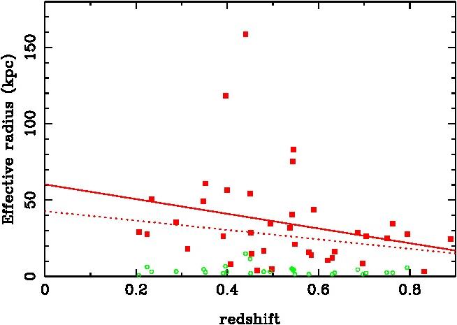
Figure 2: Variations of the Sérsic effective radii of the inner (empty green circles) and outer (red squares) components. The error bars given by the GALFIT programme are smaller than the symbols. The full red line shows the best linear fit when all the red points are included, and the dashed line the best fit after eliminating the points with an effective radius larger than 70 kpc.

One of our objectives when analysing this large sample of BCGs was to check if we could detect a variation of some of the Sérsic (or Nuker) parameters with redshift. We indeed find a variation of the effective radius $R_{e}$ of the outer component with redshift $z$, as seen in Fig. 2. As expected, the effective radius increases with decreasing redshift, agreeing with the general idea that BCGs are formed by accreting numerous galaxies in a more or less continuous way. However, there is a large scatter. When a linear fit is made between the effective radius $R_{e}$ and the redshift $z$, for the outer component we find a slope of $-48.1\pm 29.7$, an intercept of $60.3\pm 16.3$, a correlation coefficient of $-0.26$ and a probability that these two quantities are correlated P=89%. If the galaxies with an effective radius larger than 70 kpc are excluded, we find a slope of $-30.8\pm 14.5$, an intercept of $42.8\pm 8.0$, a correlation coefficient of $-0.35$ and a probability that these two quantities are correlated P=96%. For the inner component, the probability that these two quantities are correlated is only P=50%, so there is no apparent trend.

We should note that in the two clusters with the largest values of $R_{e,ext}$ extended intracluster light has been detected (MACS0416, see Montes & Trujillo 2018, and MACS1206, see DeMaio et al. 2015). In these two cases, the values of $R_{e,ext}$ are probably overestimated due to the contribution of the intracluster light (hereafter ICL).

The cosmological dimming factor makes the detection of low surface brightness features at high redshift difficult. The same source at z=0 and at z=0.8 will be 2.55 magnitudes arcsec^-2 fainter at hight redshift. Consequently, external parts of BCG profiles may be lost at high redshift.

A way to estimate this effect is to use Fig. 4, where we plot the effective surface brightness as a function of radius for our BCGs. Assuming a 2.55 magnitude dimming for a given BCG is equivalent to reducing the effective radius by 3 kpc to 10 kpc. If we now look at Fig. 2, even in the worst case (10 kpc), this is not enough to explain the decrease of the effective radius between z=0 and z=0.8 only with cosmological dimming effects.

Our results are at least qualitatively in agreement with Ascaso et al. (2011), who found an increase in the size of BCGs from intermediate to local redshift.

Lidman et al. (2013) considered a sample of 18 distant clusters with many spectroscopically confirmed cluster members, and found a major merger rate of $0.38\pm 0.14$ mergers Gyr^-1 at $z\sim 1$. Assuming that this rate continues to the present day, they find that it can explain the growth of the stellar mass in BCGs.

5 Comparison of the orientations of the BCGs and clusters

For the 28 clusters for which we analysed both the BCG properties and the galaxy distribution at very large scale (several Mpc) through density maps, we now compare the orientations of the BCG and of the cluster (at the cluster scale or at an even larger scale). For the remaining ten clusters we could not draw large scale density maps because we only had small images where the background could not be estimated sufficiently far from the cluster to estimate the significance level of the galaxy density.

The method to compute density maps is the following: first, for each cluster the galaxies located on the cluster red sequence were selected (the telescope, camera and filter set used for this purpose are indicated in the last two columns of Table 1). We then computedgalaxy density maps for these galaxies, based on an adaptive kernel technique with a generalized Epanechnikov kernel as suggested by Silverman (1986). Our method is based on an earlier version developed by Timothy Beers (ADAPT2) and further improved by Biviano et al. (1996). The statistical significance is established by bootstrap resampling of the data. A density map is computed for each new realisation of the distribution, with a pixel size of $0.001$ deg (3.6 arcsec). For each pixel of the map, the final value is taken as the mean over all realisations. A mean bootstrapped map of the distribution is thus obtained. The number of bootstraps used here is 100. More details can be found in the paper by Durret et al. (2016) from which some density maps are drawn, while the remaining density maps were computed more recently, based on data taken from CLASH.

Table 4: Comparison of the major axis position angle of 28 BCGs (PA_BCG) and large scale structures, measured anticlockwise from north. For three clusters, the PA of the cluster itself (PA_cluster) is different from that of the LSS (PA_LSS), and in these cases both PAs are given. The density maps of the clusters marked with an asterisk have already been published in Durret et al. (2016). The : sign indicates that the PA is not well determined (due to an ellipticity close to 0), and in four cases the PA is not given at all when the contours are too close to circular.

Cluster	PABCG	PALSS	PAcluster
Cl0016+16∗	56	35
A209	146	131
Cl0152∗	134	160
MACS0329	158	144
MACS0416	40	52
MACS0429	167	125:
MACS0454∗	113	150
MACS0647∗	46	90
MACS0717∗	63	122
MACS0744∗	22	96
A611	38	63
A851∗	76	$-$
LCDCS0172	1	100
MACS1115	148	147
MACS1149	131	90:	140
MACS1206∗	104	180
BMW-HRI1226∗	95	$-$
MACS1311	132:	174
Zw1332∗	59	$-$
LCDCS0829∗	30	51
MACS1621∗	78	125
OC02∗	126	90
MACS1720	177	49	150
A2261	174	91	60
MACS2129∗	81	80
RX2129	64	78
MS2137	71:	136
RX2328∗	113	$-$

Table 5: Maximum extents of the 3$\sigma$ contours of the density maps for 28 clusters. The density maps of the clusters marked with an asterisk have already been published in Durret et al. (2016).

Cluster	major axis	minor axis
	(Mpc)	(Mpc)
Cl0016+16∗	7.4	3.2
A209	3.6	1.5
Cl0152∗	2.5	2.1
MACS0329	3.8	2.0
MACS0416	4.1	2.0
MACS0429	2.0	1.6
MACS0454∗	3.9	3.4
MACS0647∗	6.8	2.2
MACS0717∗	6.0	1.8
MACS0744∗	3.8	1.5
A611	2.3	1.2
A851∗	5.9	5.9
LCDCS0172	4.9	3.2
MACS1115	5.1	1.7
MACS1149	8.6	4.0
MACS1206∗	5.7	2.4
BMW-HRI1226∗	2.3	2.0
MACS1311	2.4	1.4
Zw1332∗	5.8	5.4
LCDCS0829∗	7.5	3.3
MACS1621∗	7.6	2.1
OC02∗	6.0	4.6
MACS1720	2.9	2.2
A2261	2.9	1.8
MACS2129∗	3.7	1.6
RX2129	2.6	0.9
MS2137	1.9	1.0
RX2328∗	1.3	1.2

We initially intended to measure the major axis position angles of the BCGs (PA_BCG) with SExtractor. However, if the inner and outer isophotes are not elongated along the same PA, the final PA given by SExtractor is an average between these values. Since we wanted to compare the elongations of the outer isophotes of the BCGs to the elongations at the cluster scale or larger, we decided to use for BCGs the PA given by the IRAF task ELLIPSE, with which we also computed the BCG light profiles (see Sect. 3.1). The corresponding PAs are given in Table 4. The values of PA_BCG have typical uncertainties smaller than $\pm 10$ deg. In the cases when the BCGs appear very round, their PAs are ill-defined and noted with the : sign in Table 4.

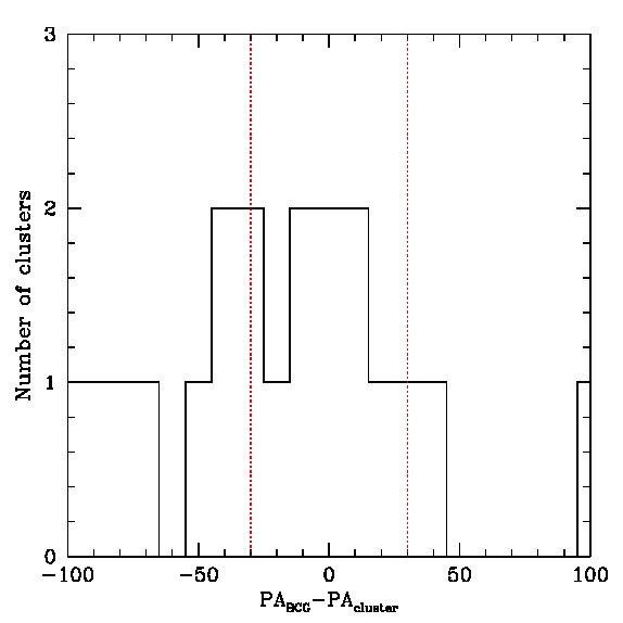
Figure 3: Histogram of the differences between the PA of the BCG and that of the LSS (or that of the cluster for the three clusters with $PA_{cluster}$ given in Table 4 for the objects with well defined BCG and large-scale structure PAs. The red lines show the limits of $\pm 30$ deg within which the PAs are considered to be compatible.

At very large scale, an indicative ellipse was adjusted by eye to the 3$\sigma$ contours of the density maps (see Durret et al. 2016), and the major axis position angles of these ellipses (PA_LSS) are also given in Table 4. Since it is necessary to extract the mean background value in the density map (far from the cluster region) to compute significance levels, such density maps were only computed for the clusters of the CLASH or DAFT/FADA surveys for which large field images (obtained with Subaru/SuprimeCam or CFHT/Megacam) were available. In view of the shapes sometimes irregular of the 3$\sigma$ contours, we estimate that the errors on PA_LSS can reach about $\pm 20$ deg. The images of the BCG of Cl0016 and its density maps are shown in Fig. 7.

The sizes of the major and minor axes of the ellipses that were fit to the $3\sigma$ contours of the large scale density maps are given in Table 5. We can see in particular the very large extent of several structures, already noted by Durret et al. (2016), and that of MACS1149, reported here for the first time.

In three cases (MACS1149, RX1720, and A2261), the PA of the cluster itself (${\rm PA_{cluster}}$) does not coincide with the PA of the elongation at a larger scale (${\rm PA_{\rm LSS}}$). In this case, we also give ${\rm PA_{cluster}}$ in Table 4.

The histogram of the values of the difference between the PA of the BCG and that of the large scale structure (in three cases, the PA of the cluster itself) is shown in Fig. 3. For two of the three clusters for which ${\rm PA_{LSS}}$ is different from ${\rm PA_{cluster}}$ (MACS1149 and MACS1720) we can note that ${\rm PA_{cluster}}$ is much closer to the value of ${\rm PA_{\rm BCG}}$ than ${\rm PA_{\rm LSS}}$. Therefore, the values of PA_BCG and either ${\rm PA_{\rm LSS}}$ or ${\rm PA_{cluster}}$ agree within less than 30 deg in 12 cases out of 21 (we count 21 objects, since out of the 28 objects, 7 have at least one of the two PAs that is ill-defined).

We now briefly consider the objects for which the BCG and larger scale PAs disagree. For MACS0717, the main cluster has several components, and PA_BCG does not seem to differ very much from that of the main western component. The BCGs of MACS1311 and MS2137 appear very round, so their PA_BCG are probably ill-defined. This is also the case for MACS1149, and besides the large scale structure shows a large curved extension, so PA_cluster is difficult to estimate. For the other clusters, the PAs appear well defined but obviously disagree.

In conclusion, out of 28 clusters, if we exclude the three BCGs with ill-defined PA_BCG and the clusters with ill-defined or undefined PA_LSS or PA_cluster (in view of their round shape), we find an agreement of the BCG and large-scale structure PAs within $\pm 30$ deg for 12 clusters out of 21.

6 Discussion and conclusions

6.1 Kormendy relation and BCG morphological parameters

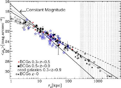
Figure 4: Effective surface brightness as a function of effective radius (Kormendy 1977 relation) drawn by Bai et al. (2014) for BCGs at various redshifts. We use their Fig. 7 as a reference, where the shaded region (here drawn with small dotted vertical lines) indicates a size that is larger than the BCG images that they used in their study; the black solid line shows the slope of the constant magnitude relation (indicated with an arrow); the other black line is the best fit to their BCG sample; the dotted line is for local BCGs and the dashed line is the best fit for the lower-mass ETGs. We superimpose as blue stars our values for the Sérsic outer component (all our objects were observed in the F814W filter except one).

Fig. 4 shows the Kormendy (1977) relation drawn by Bai et al. (2014, see their figure 7) for BCGs at various redshifts. We can see that our results for the Sérsic outer component fall quite well on this relation, though Bai et al. (2014) analysed only profiles (instead of 2D structures) and fit them by a single Sérsic law. For our 38 BCGs, the best fit corresponds to a slope of $2.64\pm 0.35$ and intercept of $19.7\pm 0.5$, with a correlation coefficient of 0.79.

This can be compared to the relation found by Kormendy (1977):

$$\mu_{B}=3.02\ logr_{0}+19.74$$ (5)

in units of B magnitudes arcsec^-2. Although the slope is somewhat different from that of the Kormendy relation, Fig. 4 shows that we overall agree.

Bai et al. (2014) found that the masses of the BCGs appear to have grown by at least a factor of 1.5 from $z=0.5$ to $z=0$, in contrast to previous findings of no evolution, and argued that such an evolution validates the expectation from the $\Lambda$CDM model. Since our results are consistent with theirs, we believe that this strengthens their conclusions. These results also agree with Burke & Collins (2013) who counted galaxies around the BCGs of 14 clusters in the redshift range $0.8<z<1.4$ and found that the BCG stellar mass could have increased by as much as a factor of 1.8 between $z=1$ and the present epoch.

We have seen in Fig. 2 that the effective radius of BCGs increases with decreasing redshift. This agrees with models of BCG formation and evolution (e.g. Aragón-Salamanca et al. 1998, De Lucia & Blaizot 2007), who found that BCGs assemble quite late (half their final mass is typically locked up in a single galaxy after z$\sim$0.5).

In a future work, we plan to estimate the masses of our 38 BCGs, to quantify the growth in mass with decreasing redshift for our sample. It would also be interesting to see if the offset of the BCG position relative to the cluster centre is correlated to the degree of concentration of cluster X-ray morphology, and to see if the brighter BCGs are preferentially found in morphologically disturbed clusters, as done by Hashimoto et al. (2014), based on ground-based data obtained with Subaru.

6.2 Preferential orientations

In Sect. 5, we have compared the PAs of the structures at different scales: PA_BCG, PA_cluster, and PA_LSS. We found an agreement of PA_BCG and PA_LSS (or in three cases PA_cluster) within $\pm 30$ deg for 12 clusters out of 21 (excluding BCGs or clusters where the PAs are ill-defined or undefined). In view of recent results by West et al. (2017), we expected that the PAs would agree for a larger number of clusters. Based on Hubble Space Telescope observations of 65 distant galaxy clusters, these authors found that giant elliptical galaxies in the centres of rich clusters often have major axes sharing the same orientation as the surrounding matter distribution on larger scales. They argued that BCGs are the product of a special formation history, influenced by the development of the cosmic web over billions of years. At lower mass, Paz et al. (2011) found an alignment of galaxy groups with the surrounding large scale structure, with a strong alignment signal between the projected major axis of group shapes and the surrounding galaxy distribution up to scales of 30 Mpc h^-1, this observed anisotropy signal becoming larger as the galaxy group mass increases.

Looking at the figures of Appendix B (right column), we can see that in 6 cases out of 17 (MACS0329, MACS0416, MACS1149, LCDCS0829, RX2129, and MS2137) the main cluster is elongated towards the other nearby structures. Plionis & Basilakos (2002) stated that clusters were aligned towards their nearest neighbour, specially within superclusters, suggesting anisotropic merging. This is probably the case in the six above-mentioned clusters, which also have properties comparable to those of the three intermediate redshift clusters studied by Foëx et al. (2017). These authors found that the optical morphology of the clusters correlates with the orientation of their BCG, and with the position of the main axes of accretion.

6.3 Relation between the BCG and the ICL

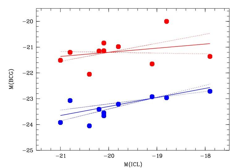
Figure 5: Absolute magnitude of the outer (blue points) and inner (red points) components of the BCG as a function of the absolute magnitude of the intracluster light for the ten clusters in common with Guennou et al. (2012). The corresponding regressions are shown as full lines and the regressions within $\pm 1\sigma$ of the best fit parameters as dotted lines (see text).

Comparing our results (Table 2) with the work of Guennou et al. (2012), we first note that all ten clusters of Guennou et al. (2012) have detected intracluster light (ICL) and that they are all better fit with two Sérsic functions. This could suggest that physical processes having created the ICL are also at the origin of an extended halo of the BCGs. In order to investigate further this possible relation, we compared for these ten clusters the total absolute magnitude of the external Sérsic component of the BCG $\rm M_{BCG,ext}$ (see Table 2) with the total absolute magnitude of the cluster ICL $\rm M_{ICL}$ from Guennou et al. (2012). Fig. 5 shows the correlation between these two components, the best fit being:

$$\rm M_{BCG,ext}=(0.35\pm 0.11)M_{ICL}-(16.3\pm 2.1).$$

As a comparison, we perform the same exercise with the total absolute magnitude of the internal Sérsic component of the BCG, and as expected we have no significant relation:

$$\rm M_{BCG,int}=(0.16\pm 0.19)M_{ICL}-(18.0\pm 3.8).$$

To explain this relation, one may argue that the ICL detected by Guennou et al. (2012) is simply a part of the external BCG halo for each cluster. However, the external BCG halos are much brighter than the detected ICL, so we are not considering the same light sources. Moreover, ICL sources are extending up to 60 kpc from the cluster centers (see Fig. 5 of Guennou et al. 2012), while the effective radii of Table 2 are in most cases lower than 30 kpc. We are therefore not sampling the same cluster areas. We therefore propose that the physical phenomena at the origin of the ICL are related to the formation of the BCG halos, both qualitatively and quantitatively.

However, based on CLASH data, Burke et al. (2015) claim that the ICL and BCG were not built up by the same mechanism. They found that minor mergers (mergers with objects with masses half of the BCG mass) are the dominant process for stellar mass assembly at low redshifts, the majority of the stellar mass from interactions contributing to the ICL, rather than building up the BCG. Therefore, their point of view is that different processes build up the ICL and BCGs. We must however note that they do not extract the ICL contribution in the same way as Guennou et al. (2012), so the results of these two papers may not be not directly comparable.

6.4 Conclusions

Our study is limited here to redshifts $z<0.9$. It would be interesting to study BCGs at larger redshifts to see if their growth can be traced at higher redshifts. Concerning the alignments of the major axes of BCGs with the elongations of larger scale structures, the study of a statistically significant sample of clusters in the present redshift range is now timely to reach conclusive results, and observations at $z>1$ would be of interest to check if the properties discussed here are also observed in the earlier universe. The implications of such a study for testing the cluster formation and evolution paradigm clearly requires larger samples and a proper comparison with cosmological simulations, and this will be the object of future work.

Appendix A Residual and sharp-divided maps

In Fig. 6, we show for the BCG of Cl0016 analysed with GALFIT the map of the residuals obtained after subtracting to the BCG its best fit (by the sum of two Sérsic models), and the corresponding sharp divided image, in the F814W band. The sharp divided image was mainly used to identify correctly the objects that needed to be masked in order to obtain the best possible fit of the BCGs. The maps of the residuals obtained by subtracting to the BCGs its best fits (by a single Sérsic model, by the sum of two Sérsic models, or by the sum of a Sérsic and a Nuker models) for all the clusters of our sample and the corresponding sharp divided images are available on this link : ftp://ftp.iap.fr/pub/from_users/durret/BCGs/Durret_BCGs.pdf

Cl0016: the residuals are very faint, showing that the fit is good. The sharp divided image seems to show a diffuse halo around the BCG.

A209: the residuals show matter in the very centre of the BCG as well as in its outskirts.

Cl0152: here also there is matter left in the central part of the galaxy.

MACS0329: a relatively bright feature extends up to about 20 kpc north-west of the BCG centre.

MACS0416: some large scale diffuse emission is seen around the BCG.

MACS 0429: besides possible diffuse light at large scale, there are many features in the BCG area.

MACS0454: the fit is very good except in the very central regions of the BCG.

MACS0647: an excess is visible near the BCG centre.

MACS 0717: an excess is visible near the BCG centre.

MACS0744, A611, A851, LCDCS0110, LCDCS0130: same as Cl0016.

LCDCS0172: the fit to the BCG is not perfect, probably due to the presence of a small galaxy a few kpc north of the BCG.

LCDCS0173, Cl1103, MACS1115, LCDCS0340: same as Cl0016.

MACS1149: an elongated emission region crosses the BCG in the north-west to south-east direction.

MACS1206, LCDCS0504, BMW1226, LCDCS0531: same as Cl0016.

LCDCS0541: the fit is not perfect.

MACS1311: same as Cl0016.

Zw1332: the fit is good, and the sharp divided image reveals faint features south-west and north-east of the BCG centre.

LCDCS0829 (RX1347), LCDCS0853: the fit is not perfect, and large diffuse emission is visible.

MACS1621: the fit is very good.

OC02: the fit is not perfect, and some diffuse emission is visible.

MACS1720: same as Cl0016.

A2261: same as Cl0016 though the fit is not perfect.

MACS2129: the fit is not perfect.

RX2129, MS2137, RX2248: same as Cl0016.

RX2328: an elliptical residual is clearly seen in the central zones of the BCG

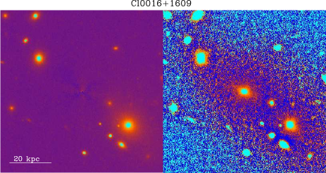
Figure 6: Left: residuals after fitting Cl0016 with two Sérsic profiles. Right: sharp divided image of the BCG of Cl0016. The two images have identical scales. North is top and East is left.

Appendix B Comparison of the orientations of the BCGs and clusters

In Fig. 7 we show for the cluster Cl0016 the image of the BCG and of the large scale structure around the cluster. As mentioned in Appendix A, these figures for all the clusters are available on this website : ftp://ftp.iap.fr/pub/from_users/durret/BCGs/Durret_BCGs.pdf. Some of the large scale density maps have already been published in Durret et al. (2016) but we show them again for easy comparison with the BCG. In some cases, we zoomed them to show only the cluster and its immediate surroundings. Some regions labeled on the density maps (A, B…) are the same as in Durret et al. (2016).

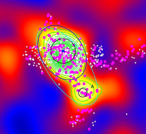
Figure 7: Cl0016+1609. Left: image of the BCG. The BCG is indicated with a red cross, the small galaxy to the north-east belongs to the cluster, but not the large galaxy located south-west of the BCG. Right: large scale density map computed from the galaxies located on the cluster red sequence. The black circle is centred on the position of the cluster given in Table 1 and has a 1 Mpc radius, as in all following figures (in some cases, the circle is drawn in another colour to be more visible). In both figures, the contour levels start at $3\sigma$, they increase by $2\sigma$ or $3\sigma$ in the left figures, depending on the brightness of the BCG, and by $1\sigma$ in the density maps. In the right figure, the ellipse (here in cyan, but drawn with different colours for other clusters to be clearly visible) indicates the maximum extent of the $3\sigma$ contours. The small green or white points show the positions of the galaxies with a measured spectroscopic redshift. The magenta points show the galaxies with redshifts in the approximate cluster redshift range (this range is indicated in the figure caption of each cluster, it is $0.53<z<0.57$ for Cl0016+1609), and the small blue rectangle at the centre shows the size of the left figure (in this and following figures). North is up and east is left in all figures.