Quasiparticle Bound States around Fractional Vortices in $s$-wave Superconductor

Abstract

Since the experimental formation of a vortex with a fractional quantized magnetic flux in a thin superconducting $s$-wave bi-layer was recently reported, we calculate the local density of states (LDOS) around two half quantum vortices in a $s$-wave superconductor on the basis of the quasiclassical Eilenberger theory to investigate the effect of the phase discontinuity. We show that the LDOS pattern around fractional vortices is qualitatively different from that around conventional vortex. We find that the novel bow-tie-shaped bound states appear in the high energy region, which can be an evidence for the fractional vortices through scanning tunneling microscopy/spectroscopy. We also show that the system with $n$ fractional vortices with the vorticity $1/n$ has a similarity to the Josephson junctions.

I Introduction

Recently, Tanaka et al. reported observation of fractionalization of magnetic flux $\Phi_{0}$ in a thin superconducting Nb bi-layer Tanaka through magnetic field distribution image taken by a scanning superconducting quantum interference device (SQUID) microscope. As an earlier relevant study, Moler’s group reported signature for phase soliton TanakaPRL and fractionally quantized flux in the pattern of current as a functional of the applied flux in superconducting aluminum rings of various sizes Moler2006 . Her group also reported sub-$\Phi_{0}$ features in highly underdoped cuprate superconductors YBCO and they attributed it to the kinked stacks of pancake vorticesMoler2008 . The authors in Ref. Tanaka claimed that fractional vortices in their system are explained by a multi-component $s$-wave conventional superconductivity.

The term “fractional vortex”, however, has been used in two ways: fractionally-quantized-flux vortex and/or fractional-phase vortex. The former is the vortex whose magnetic flux is fractionally quantized and the latter is the vortex whose superconducting phase is fractional. In both cases, the magnetic flux of a vortex is fractionally quantized. Fractionally-quantized-flux vortices have been discussed in multi-component superconductorsTanakaPRL ; Babaev ; Lin . Machida et al. suggested that half fractionally-quantized-flux vortices spontaneously emerge in corners of $d$-wave superconductor dot embedded in $s$-wave superconducting matrix due to the phase interference between superconducting order parameters with different symmetries.Machida Fractional-phase vortices has been discussed by Volovik in chiral superfluids and superconductorsVolovik . The half quantum phase vortices are allowed in the triplet superfluids due to their spin degrees of freedom. The stability of the half quantum vortices have been discussed in $p_{x}+ip_{y}$ superconductors by Chung et al.Chung They showed that the stability of two half quantum vortices is enhanced when the ratio of spin superfluid density to superfluid density is small.

The observation of fractional quantized magnetic flux in the bi-layer $s$-wave superconductor does not necessarily mean the existence of the latter fractional vortex, a fractional-phase one, since the SQUID experiment can not measure the phase of the order parameter. Thus, another experimental measurement is needed to conclude which fractional vortex appears in the bi-layer $s$-wave superconductor. Through out this paper, we use “fractional vortex” as the fractional-phase vortex.

The quasiparticle bound states around a vortex reflects the pairing symmetry.Caroli ; Ichioka ; Hayashi ; Nagai ; Nagaitopo ; Bao The local density of states (LDOS) around a vortex has been investigated in various superconductors such as $s$-wave, anisotropic $s$-wave and $d$-wave superconductors. The LDOS can be observed by the scanning tunneling microscopy/spectroscopy (STM/STS) Hess ; Nishimori ; Tao . In the system with conventional vortices, the phase of the pair-potential changes $2\pi$ around a vortex, so that quasiparticles feel $\pi$-shift of pair-potential running through a vortex core. In the system with the half quantum vortices, there is the phase discontinuity, so that the shape of the quasiparticle bound states around these fractional vortices is nontrivial.

The purpose of this paper is to investigate the quasiparticle bound states around fractional vortices in $s$-wave superconductor. For simplicity, we consider the single-band isotropic $s$-wave superconductor with the two-dimensional isotropic Fermi surface on the basis of quasiclassical Eilenberger theoryEilenberger ; Larkin . It is appropriate to investigate the phase discontinuity. We consider two kinds of the system with half vortices. The former is the system with “isolated” fractional vortices, where the gap amplitude on the line between two half vortices is not zero (See, Fig. 1(a)). The latter is the system with “connected” fractional vortices, where the gap amplitude on the line between two half vortices is zero (See, Fig. 1(b)). We discuss how to obtain the evidence for the fractional vortices.

This paper is organized as follows. The model and method are shown in Sec. II. The systems with the isolated fractional vortices are shown in Sec. III. In this section, we consider the two half vortices and $n$ fractional vortices with vorticity $1/n$. The system with the two connected fractional vortices is shown in Sec. VI. The discussion is given in Sec. V. The conclusion is given in Sec. VI.

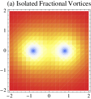
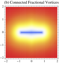
Figure 1: (Color online) Schematic figures of a spatial dependence of the gap amplitude $f(\mbox{\boldmath$r$})$ with two half vortices. (a)“Isolated” denotes that $f(\mbox{\boldmath$r$})\neq 0$ on the branch cut. (b) “connected” denotes that $f(\mbox{\boldmath$r$})=0$ on the branch cut.

II Model and Method

We use the quasiclassical theory developed by Eilenberger, Larkin and Ovchinnikov Eilenberger ; Larkin , which is suited to discuss most superconductors. We consider two-dimensional clean superconductors with isotropic Fermi surface in the type II limit for simplicity and we ignore the self-energy part of Green function and the vector potential.

We discuss LDOS $\nu(\epsilon,{\bm{r}})$ for quasiparticles with excitation energy $\epsilon$ at each position $\bm{r}$ around fractional vortices. For our purpose, it suffices to calculate diagonal part (in particle-hole space) of quasiclassical Green function $g(\epsilon+{\rm i}0,\hat{\bm{k}})$ as a function of $\epsilon$ and the position on the Fermi surface (denoted by a two-dimensional unit vector $\hat{\bm{k}}$). The LDOS follows from $g$ averaged over the Fermi surface $\langle\cdots\rangle_{\hat{\bm{k}}}$,

$$\nu(\mbox{\boldmath$r$},\epsilon)=-\nu(0)\langle{\rm Re}\;g(\epsilon+{\rm i}\delta,\hat{\bm{k}})\rangle_{\hat{\bm{k}}},$$ (1)

where $\nu(0)$ denotes the density of states on Fermi surface in the normal metallic state.

The equation of motion for $g$ is called Eilenberger equation, which can be simplified by introducing auxiliary functions $a$ and $b$ defined by

$$g=-\frac{1-ab}{1+ab}.$$ (2)

The auxiliary functions $a$ and $b$ satisfy

$$\mbox{\boldmath$v$}_{\rm F}\cdot\mbox{\boldmath$\nabla$}a+2\omega_{n}a+a\Delta^{\ast}(\bm{r})a-\Delta(\bm{r}) = 0,$$ (3)

$$\mbox{\boldmath$v$}_{\rm F}\cdot\mbox{\boldmath$\nabla$}b+2\omega_{n}b-b\Delta(\bm{r})b+\Delta^{\ast}(\bm{r}) = 0,$$ (4)

which is Eilenberger equation in Riccati formalismNagato ; Schopohl . Here $\mbox{\boldmath$v$}_{\rm F}=v_{\rm F}\hat{k}$ denotes the Fermi velocity and $\Delta(\bm{r})$ the gap function. We use the analytic continuation $i\omega_{n}\rightarrow\epsilon+{\rm i}\delta$ when we calculate the LDOS. Since these equations (3) and (4) contain $\nabla$ only through $\mbox{\boldmath$v$}_{\rm F}\cdot\mbox{\boldmath$\nabla$}$, they reduce to a one-dimensional problem on a straight line, the direction of which is given by that of the Fermi velocity $\mbox{\boldmath$v$}_{\rm F}$.We calculate the LDOS by solving (3) and (4) with the fourth order Runge-Kutta method. For simplicity, we defined the gap function $\Delta(\mbox{\boldmath$r$})$ without self-consistent gap equation.

There are branch cuts between fractional vortices. Crossing the branch cut, the phase $\arg(\Delta(\mbox{\boldmath$r$}))\equiv\phi$ changes $\pi/n$. Here, $n$ denotes an inverse of a vorticity (i.e., $n=2$ with two half vortices). We consider two cases about a spatial dependence of the gap amplitude. In the former case, we consider “isolated” fractional vortices, where the gap amplitude $|\Delta(\mbox{\boldmath$r$})|\equiv f(\mbox{\boldmath$r$})\neq 0$ on the branch cut between each isolated fractional vortex as shown in Fig. (1)(a). In the latter, we consider “connected” fractional vortices, where $f(\mbox{\boldmath$r$})=0$ on the branch cut between each connected fractional vortices as shown in Fig. (1)(b).

III Isolated Fractional Vortices

III.1 Two Half Vortices

Figure 2: Frame of the space with two half vortices. $\delta$ is the inter-vortex distance. $\theta_{r}$ is the angle between the $a$ axis and $r$.

We consider the system with the two isolated half fractional vortices. Here, the origin is at a midpoint between half vortices(See, Fig. 2 and our previous paperNagai ). We denote by $X,Y$ a Cartesian coordinate in a laboratory frame (and we reserve the symbols $x$ and $y$ as the coordinate for $\hat{\bm{k}}$ dependent-frame). We consider the pair function of the two isolated half fractional vortices written as

$$\frac{\Delta(r)}{\Delta_{\infty}} = f_{+}(X,Y)f_{-}(X,Y)\exp[i(\phi_{+}(X,Y)+\phi_{-}(X,Y))],$$ (6)

$$\equiv f(r)\exp[i\phi(r)],$$

where

$$f_{\pm}(X,Y) = \tanh^{1/2}(\sqrt{(X\pm\delta)^{2}+Y^{2}}),$$ (7)

$$\phi_{\pm}(X,Y) = \arctan(Y/(X\pm\delta))/2,$$ (8)

as shown in Fig. 1(a). $\Delta_{\infty}$ denotes the modulus of the gap function far away from the vortices. Here, $\delta$ denotes the inter-vortex distance. The phase $\phi(r)$ changes $\pi/2$ crossing the branch cut between two half vortices.

Figure 3: (Color Online) Local density of the states in the system with two isolated half fractional vortices. The inter-vortex distance $\delta=0.8\xi_{0}$. The distributions of the LDOS on the left hand side and the sets of the quasiparticle paths on the right hand side. (a) and (d):the energy $\epsilon=0.1\Delta_{\infty}$, (b) and (e): the energy $\epsilon=0.4\Delta_{\infty}$ and (c) and (f):the energy $\epsilon=0.9\Delta_{\infty}$. the smearing factor $\eta=0.001\Delta_{\infty}$.

III.1.1 Numerical Results

We calculate the LDOS with $\delta=0.8\xi$ numerically as shown in Fig. 3(a)-(c). The LDOS patterns can be divided into three energy regions. In the low energy region as shown in Fig. 3(a) ($\epsilon\gtrsim 0.3\Delta$), the LDOS pattern is quite different from that around a single vortex. The LDOS around a single vortex has a circular pattern and the peak position of this LDOS is located near the center of the vortex core. In contrast, the peak positions of the LDOS with the half vortices are located at $(X,Y)\sim(\pm 0.3\xi_{0},0)$, whose points are near the midpoint between two half vortices. In the middle energy region ($0.3\Delta\gtrsim\epsilon\gtrsim 0.8\Delta$), the LDOS patterns change from that like the triangular to that like the ellipse. We show the LDOS with the energy $\epsilon=0.4\Delta$ in Fig. 3(b). In the high energy region, the novel quasiparticle bound states are found inside the conventional circular LDOS pattern (See, Fig. 3(c)).

In the quasiclassical theory, the equations of motion for quasiparticles running in a certain direction can be respectively solved since we assume the non-selfconsistent gap function as shown in Eqs. (3), (4) and (6). Therefore, results can be respectively explained by the enveloping curves of the set of quasiclassical paths.Nagai We draw the set of quasiclassical paths as shown in Fig. 3(d)-(f). We can show that the analysis by the quasiparticle paths used in our previous paperNagai can be applied to the analysis of the LDOS by the numerical method. In the following sections, we explain the origins of the LDOS patterns in the each energy region.

III.1.2 Low Energy Region

The features of the LDOS pattern in this energy region are that the low energy LDOS pattern is like a triangular shape (See, Fig. 4(a)) and that the peak positions of the LDOS with the half vortices are located near the midpoint between two half vortices. Around a single vortex, the LDOS has a circular symmetric pattern and the peak position of this LDOS is located near the center of the vortex core.

We show the energy dependence of the peak positions for the quasiparticles running in the $Y$-direction are shown in Fig. 6(a). $y$ in Fig. 6(a) denotes an impact parameter, which is equal to $X$ as shown in Fig. 5. Therefore, these peak positions shift away from the origin with increasing the energy.

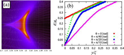
Figure 4: (Color Online)(a): The local density of the states in the system with two isolated half fractional vortices at the energy $\epsilon=0.1\Delta_{\infty}$. This figure is the enlargement of Fig. 3(a). (b)The energy dependence of the peak positions for quasiparticles in the various directions.

Figure 5: Frame of the space with $\theta=\pi/2$.

This feature is explained on the basis of the Kramer-Pesch approximation, which is appropriate in the low energy region.Nagai ; Kramer This approximation is the perturbation theory where the denominator of the Green function around the origin is expanded with respect to $y$ and an energy $\omega_{n}$. On the $Y$-axis, we can easily solve Eqs. (3),(4), since the phase of the pair-function $\phi(0,Y)$ changes only at the origin from $3\pi/2$ to $\pi/2$. The Green function at the origin is written as

$$g(\mbox{\boldmath$r$}=0;i\omega_{n}) = -\frac{1-a(x\rightarrow-\infty)b(x\rightarrow\infty)}{1+a(x\rightarrow-\infty)b(x\rightarrow\infty)},$$ (9)

$$= -\frac{(\omega_{n}+\sqrt{\omega_{n}^{2}+|\Delta_{\infty}|^{2}})^{2}+|\Delta_{\infty}|^{2}}{(\omega_{n}+\sqrt{\omega_{n}^{2}+|\Delta_{\infty}|^{2}})^{2}-|\Delta_{\infty}|^{2}}.\>\>\>\>\>\>\>$$ (10)

This Green function diverges at the zero energy ($i\omega_{n}=0$) so that the Andreev bound states occur at the zero energy at the origin. We consider this Green function as an unperturbed Green function. Let us expand the pair function $\Delta(x,y)=f(x,y)\exp(i\phi(x,y))$ with respect to $y$ near the origin. We can regard as $f(x,y)\sim const.$ when the inter-vortex distance is large. The phase $\phi$ is expressed as

$$\phi(x>0) = \frac{3\pi}{2}+\frac{\delta\theta_{1}+\delta\theta_{2}}{2},$$ (11)

$$\phi(x<0) = \frac{\pi}{2}-\frac{\delta\theta_{1}+\delta\theta_{2}}{2}.$$ (12)

Here, $\delta\theta_{1}$ and $\delta\theta_{2}$ are defined as shown in Fig. 5. In the first order with respect to $y$, $\exp(i\phi(x))$ is written as

$$e^{i\phi(x)}\sim-{\rm sign}\>(x)\exp\left({\rm i}\frac{\pi}{2}\right)\left(1+{\rm i}\frac{x}{\delta^{2}+x^{2}}y\right).$$ (13)

Then, we obtain the pair function $\Delta(x,y)$ with respect to $y$:

$$\Delta(x,y) \sim -\Delta_{\infty}{\rm sign}\>(x)\exp\left({\rm i}\frac{\pi}{2}\right)\left(1+{\rm i}\frac{x}{\delta^{2}+x^{2}}y\right),$$ (15)

$$= \Delta_{0}+{\rm i}\frac{x}{\delta^{2}+x^{2}}y\Delta_{0}.$$

Here, $\Delta_{0}=-\Delta_{\infty}{\rm sign}\>(x)\exp\left({\rm i}\frac{\pi}{2}\right)$. In the Kramer-Pesch approximation about a single vortex, the first order of the pair function is expressed as $\Delta_{1}=iy/x\Delta_{0}$. Therefore, as in the Ref. Nagai, , the energy dependence of the peak position for the quasiparticles running in the $Y$-direction is written as

$$y\propto\epsilon.$$ (16)

This relation means that, with increasing the energy, the quasiparticle path shifts away from the origin, so that the peak positions of quasiparticle bound states also shift away from the origin on the $X$-axis.

As shown in Fig. 4(a), the low energy LDOS pattern is like a triangular shape. This shape is explained by the set of the quasiparticle paths shown in Fig. 3(d). The quasiparticles can not run in the $X$-direction, since the quasiparticle path in the $X$-direction does not exist as shown in Fig. 3(d). In the energy range $\epsilon<0.3\Delta_{\infty}$, the quasiparticles running such a direction is not allowed, since these quasiparticles have the gap as shown in Fig.6(b). We show the energy dependence of the peak positions for quasiparticles running in the various directions ($\theta$) in Fig. 4(b). In the energy $\epsilon=0.1\Delta_{\infty}$, the impact parameters $y$ for quasiparticles in Fig. 4(b) are small. Therefore, the quasiparticles can not form the circler symmetric LDOS pattern. The dispersion relation of the quasiparticle running in the $X$-direction shown in Fig.6(b). In Figs. 3(d)-(f), the set of quasiparticle paths are drawn calculating the energy dispersion relations of the quasiparticles running in the various directions.

Figure 6: Energy dependence of peak positions for the quasiparticle running in the (a):$Y$ direction and (b):$X$ direction with isolated two half vortices.

III.1.3 Middle Energy Region

At the gap energy $\epsilon\sim 0.3\Delta$, the LDOS patterns change from that like the triangular to that like the ellipse. We show the LDOS with the energy $\epsilon=0.4\Delta$ in Fig. 3(b). In this middle energy region, the quasiparticles do not cross the branch cut ($-\delta<X<\delta$) as shown in Fig. 3(e). On the other hand, the quasiparticles cross the branch cut as shown in Fig. 3(d) in the low energy region. We show the energy dependence of the LDOS at the half fractional vortex core ($X=\delta=0.8\xi$) in Fig. 7.

Figure 7: Energy dependence of the LDOS at the half fractional vortex core.

In the energy $\epsilon=0.33\Delta$, the LDOS at the half vortex core diverges. This result shows that the peak position cross a vortex core with increasing energy.

As shown Fig. 4(b), the energy dependence of peak positions in the various directions in this middle energy region can be written as

$$\epsilon\sim c_{1}y+c_{0}.$$ (17)

Here, $c_{0}$ and $c_{1}$ do not depend on the angle $\theta$. Therefore, the ellipsoidal LDOS patterns are in proportion to the energy in this energy region.

III.1.4 High Energy Region

In the high energy region, the novel quasiparticle bow-tie-shaped bound states are found inside the conventional circular symmetric LDOS pattern (See, Fig. 3(c)). As shown in Fig. 6(b), another branch in the high energy region appears in the energy dependence of peak positions for the quasiparticles running in the $X$ direction. We show the energy dependence of the retarded Green function in the $X$ direction in Fig. 8(a). In this figure, two Andreev bound states are clearly observed under the gap energy. The bow-tie-shaped Andreev bound states with a high energy are near the origin as shown in Figs. 3(c) and (f). The LDOS pattern in the high energy region are the superposition of the bow-tie-shaped pattern and the circular pattern, since the quasiparticle paths of the each pattern are superposed as shown in Figs. 3(f).

One can observe the LDOS pattern as the evidence of the fractional vortices in the high energy region rather than the low energy region. In the low energy region, the novel bound states are located between two half vortices, so that one has to observe it precisely. One can easily observe the bow-tie-shaped LDOS patterns in high energy region by STM/STS since the novel bound states in this region are larger than the two half vortices.

III.1.5 Dependence of the inter-vortex distance

The inter-vortex distance $\delta$ depends on the free-energy in the real materials. We investigate the energy dependence of peak positions for the quasiparticles running in $X$-direction as shown in Fig. 8(b) with increasing the inter-vortex distance. In the conventional single vortex limit ($\delta\rightarrow 0$), there is the one conventional Andreev bound states at the zero energy. With increasing the inter-vortex distance $\delta$, the energy of the novel bound states become small and the energy of the lower bound states become large. In the large inter-vortex distance limit ($\delta\rightarrow\infty$), these two dispersion curves merge.

Figure 8: (a):Energy dependence of the retarded Green function in the $X$-direction near the origin. (b) the inter-vortex distance dependence of peak positions for the quasiparticles in the $X$-direction.

These results suggest that the high-energy novel bound states appear in the region $\delta>0.25\xi$.

We show that these novel bound states also appear in the the zero-core (phase vortex) model, where only the phase of the pair-potential spatially changes and the amplitude of that does not change. In the zero-core model, we can solve Eqs. (3),(4) on the $X$-axis analytically. We derive the $X$-line into A, B and C segments as shown in Fig. 9. The initial conditions of the variables $a_{\rm I}$ and $b_{\rm I}$ of the Riccati equations (3) and (4) are written as

$$a_{\rm I}(X\rightarrow-\infty) = e^{i\pi}(-\omega_{n}+\sqrt{\omega_{n}^{2}+1}),$$ (18)

$$b_{\rm I}(X\rightarrow\infty) = (-\omega_{n}+\sqrt{\omega_{n}^{2}+1}).$$ (19)

Here, we use dimensionless variables as $\omega_{n}/\Delta_{\infty}\rightarrow\omega_{n}$, $X/\xi_{0}\rightarrow X$. We can solve Eqs. (3),(4) since the equations are $n=2$ Bernoulli Equations in each segment. With the use of the particular solution in the segment B written as

$$a_{\rm Bp}=e^{\frac{\pi}{2}i}(-\omega_{n}+\sqrt{\omega_{n}^{2}+1}),$$ (20)

the general solutions in the system with the half phase vortices are written as

$$a_{\rm Bg}(X) = \frac{-i+e^{c(X+\delta)}(-1+(1+i)\omega_{n}(c/2-\omega_{n}))}{(1+e^{c(X+\delta)})c/2+\omega_{n}(-1+e^{c(X+\delta)})},\quad$$ (21)

$$b_{\rm Bg}(X) = -a_{\rm Bg}(-X),$$ (22)

where $c=2\sqrt{\omega_{n}^{2}+1}$. Then, we obtain the Green function from Eqs. (2),(21) and (22). Figure 10(a) shows the energy dependence of the retarded Green function. This result is consistent with the numerical calculation as shown in Fig. 8(a). The bound energy is obtained by the solution of the equation:

$$i\epsilon(c^{\prime}+(4\epsilon-4\epsilon^{3}-c^{\prime})e^{2c^{\prime}\delta})=0,$$ (23)

where $c^{\prime}=2\sqrt{1-\epsilon^{2}}$ and $i\omega_{n}\rightarrow\epsilon+i\eta$ $(\eta\rightarrow+0)$. Therefore, the inter-vortex distance dependence of the peak position on the $X$-axis is written as

$$\delta=-\frac{\log(-2\epsilon\sqrt{1-\epsilon^{2}}+1)}{4\sqrt{1-\epsilon^{2}}}.$$ (24)

At the energy $\epsilon=1/\sqrt{2}$, the inter-vortex distance $\delta$ diverges as shown in Fig. 10(b).

Figure 9: Spatial dependence of the phase of the pair-potential of the quasiparticle on the $X$ axis in the system with the half phase vortex.

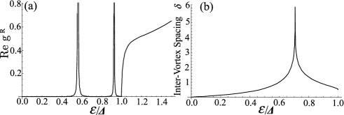
Figure 10: Inter-vortex distance dependence of peak positions for the quasiparticle running on the $X$ axis in the system with the phase vortices.

III.2 $n$ Fractional Vortices with Vorticity $1/n$

We also calculate the energy dependence of the Andreev bound states in the system with $n$ fractional vortices with vorticity $1/n$ on the $X$ axis to investigate the effects of the vorticity. We assume the zero-core model (phase vortex model) and consider the frame of the space as shown in Fig. 11.

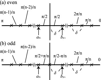
Figure 11: Spatial dependence of the phase of the pair-potential of the quasiparticle on the $X$ axis in the system with the half phase vortex.

Figure 12 shows the inter-vortex distance dependence of peak positions relations in the case of $n=3,4$ with the numerical calculations. Three and four bound states appear, respectively. In the large inter-vortex distance limit, the bound energy is

$$\epsilon_{\rm 1/3,num}/\Delta = 0.864\pm 0.005,$$ (25)

$$\epsilon_{\rm 1/4,num}/\Delta = 0.927\pm 0.005.$$ (26)

As the case of the half vortices, we solve the Riccati equations (3) and (4) analytically. In the long inter-vortex distance limit, the solutions $a$ and $b$ in each segment are equal to the bulk-solutions written as

$$\partial a/\partial X=\partial b/\partial X=0.$$ (27)

The energy of the bound states is obtained by solving the equation written as

$$\sqrt{1-\epsilon^{2}}+\sqrt{1-\epsilon^{2}}\cos\frac{\pi}{n}+\epsilon\sin\frac{\pi}{n}$$

$$+i\left(-\epsilon+\sqrt{1-\epsilon^{2}}\sin\frac{\pi}{n}+\epsilon\frac{\pi}{n}\right)=0.$$ (28)

Therefore, we obtain the energy of the bound states written as

$$\epsilon=\cos\left(\frac{\pi}{2n}\right).$$ (29)

In the case of $n=3,4$, the bound energies are

$$\epsilon_{\rm 1/3,ana} = \cos\left(\frac{\pi}{6}\right)\sim 0.866025\sim\epsilon_{\rm 1/3,num},$$ (30)

$$\epsilon_{\rm 1/4,ana} = \cos\left(\frac{\pi}{8}\right)\sim 0.92388\sim\epsilon_{\rm 1/4,num},$$ (31)

respectively.

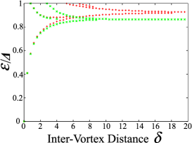
Figure 12: (Color Online) (a)Energy dependence of the retarded Green function in the $X$-direction. (b):The inter-vortices dependence of the dispersion relation of the quasiparticle running on the $X$ axis in the system with the phase vortices.

These results can be understood by the analogy of the Josephson junctions. In this limit, the quasiparticles running on $X$ axis pass through the single vortex with vorticity $1/n$. Therefore, we can regard this single vortex as the single Josephson junction between the superconductors with different phase of the pair-potential. The bound energy at the junction between two superconductors with the phase difference $\Delta\phi=\pi/n$ is written as

$$\epsilon=\cos\left(\frac{\Delta\phi}{2}\right)=\cos\left(\frac{\pi}{2n}\right).$$ (32)

IV Connected Fractional Vortices

IV.1 Two Half Vortices

We consider the pair function of the two connected half fractional vortices is written as

$$\Delta(r) = f_{0}(X,Y)\exp[i(\phi_{+}(X,Y)+\phi_{-}(X,Y))],$$ (34)

$$\equiv f_{0}(r)\exp[i\phi(r)],$$

where

$$f_{0}(X,Y) = \left\{\begin{array}[]{ll}\sqrt{\tanh(|Y|)f_{+}(X,Y)},&\quad-X_{+}<X<0\\ \sqrt{f_{-}(X,Y)\tanh(|Y|)},&\quad 0<X<X_{+}\\ \sqrt{f_{-}(X,Y)f_{+}(X,Y)},&\quad|X|>X_{+}\end{array}\right.$$ (38)

$$f_{\pm}(X,Y) = \tanh(\sqrt{Y^{2}+(X\mp X_{+})^{2}})$$ (39)

$$\phi_{\pm}(X,Y) = \arctan(Y/(X\pm\delta))/2.$$ (40)

As shown in Fig. 1(b), the gap amplitude on the branch cut is zero.

IV.1.1 Local Density of States

We calculate the local density of states with two connected half vortices. As shown in Fig. 13, the LDOS with two connected half vortices is similar to that with two isolated half vortices shown in Fig. 3 qualitatively. This result suggests that the appearance of the bow-tie-shaped bound states in the high energy region does not depend on the details of the distribution of the gap amplitude.

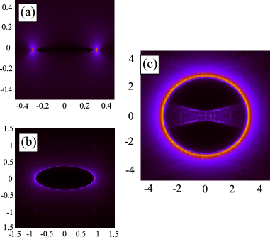
Figure 13: (Color Online) Local density of the states in the system with two connected half fractional vortices. The inter-vortex distance $\delta=0.8\xi_{0}$. (a):the energy $\epsilon=0.1\Delta_{\infty}$, (b): the energy $\epsilon=0.4\Delta_{\infty}$ and (c):the energy $\epsilon=0.9\Delta_{\infty}$. the smearing factor $\eta=0.001\Delta_{\infty}$.

IV.1.2 Energy dependence of the bound states

We obtain the energy dependence of the bound states as shown in Fig. 14.

Figure 14: Energy dependence of peak positions for the quasiparticle running in the (a):$Y$ direction and (b):$X$ direction with connected two half vortices.

Figure 15: (a):Energy dependence of the retarded Green function in the $X$-direction near the origin ($y=0.01\xi_{0}$). (b) the inter-vortex distance dependence of the energy of the bound states.

The energy dependence of peak positions for the quasiparticles running in the $Y$-direction with two connected half vortices is similar to that with two isolated half vortices. On the other hand, the quasiparticles running in the $X$-direction do not have the gap. The bound states for these quasiparticles appear in the high-energy region as shown in Fig. 15(a). The pair function on the $Y$ axis with connected vortices is similar to that with isolated vortices. On the $X$ axis, however, the pair function with connected vortices is zero on the segment between two vortices. The inter-vortex distance dependence of the bound energy for these quasiparticles is shown in Fig. 15(b). With increasing the inter-vortex distance $\delta$, the several bound states appear. For the quasiparticles running on $X$-axis, such a pair amplitude is similar to that of the S/N/S junction where the length of the normal state $L$ is $L=2\delta$. Therefore, many bound states appear when the length of the normal state region $L$ becomes large.

V Discussion

We do not solve the gap equation self-consistently for simplicity. In the real materials, we do not know whether the pair-amplitude on the branch cut is zero (isolated vortices) or not (connected vortices). However, we show that the appearance of the bow-tie-shaped LDOS pattern in the high energy region is robust against the spatial dependence of the pair-amplitude. This result suggests that the topological effects of the fractional vortices cause the bow-tie-shaped LDOS pattern in the high energy region.

With the use of quasiclassical Eilenberger theory, we can separately consider each quasiparticles with certain momentum $k$. Therefore, we can suggest that the quasiparticles running through both half vortices form the novel bound states in the high energy region ($\Delta_{\infty}\gtrsim\epsilon\gtrsim 0.8\Delta_{\infty}$) in unconventional superconductors.

VI Conclusion

In conclusion, we investigated the local density of states around two half vortices. We studied the isolated and connected two half vortices, respectively. We obtained the novel bound states in the high energy region in both cases. With increasing energy, the LDOS pattern changes from the triangular-like pattern to the ellipsoidal pattern. In the high energy region, the novel bow-tie-shaped LDOS pattern is inside the circular LDOS pattern. We showed that the LDOS patterns by the numerical method can be understood by the enveloping curve of the quasiparticle paths. We also showed that the appearance of these novel bound states does not depend on the details of the gap-amplitude distribution. These results suggest that these novel LDOS pattern can be observed by the STM/STS. We also calculate the quasiparticle dispersion in the system with isolated $n$ fractional vortices with $1/n$ vorticity. We noted that $n$ fractional vortices with $1/n$ vorticity is similar to the multi Josephson junctions.

References

- (1) Y. Tanaka, H. Yamamori, T. Yanagisawa, T. Nishio, S. Arisawa, Physica C 548, 44 (2018).
- (2) Y. Tanaka, Phys. Rev. Lett. 88, 017002 (2002).
- (3) H. Bluhm, N C. Koshnick, M. E. Huber, and K. A. Moler, Phys. Rev. Lett. 97 237002 (2006).
- (4) J. W. Guikema, H. Bluhm, D. A. Bonn, R. Liang, W. N. Hardy, and K. A. Moler, Phys. Rev. B 77 104515 (2008) .
- (5) E. Babaev, Phys. Rev. Lett. 89, 067001 (2002).
- (6) S. -Z. Lin, J. Phys. 26, 493202 (2014).
- (7) M. Machida T. Koyama, M. Kato, T. Ishida, Physica C, 412-414, 367 (2004).
- (8) G. E. Volovik, PNAS, 97, 2431 (2000).
- (9) S. B. Chung, H. Bluhm and E-A. Kim, Phys. Rev. Lett. 99, 197002 (2007).
- (10) C. Caroli, P. G. de Gennes and J. Matricon, , Phys. Lett. 9 (1964) 307.
- (11) N. Hayashi, M. Ichioka and K. Machida, Phys. Rev. B 56 (1997) 9052.
- (12) M. Ichioka, N. Hayashi, N. Enomoto and K. Machida, Phys. Rev. B. 53 (1996) 15316.
- (13) Y. Nagai, Y, Ueno, Y. Kato and N. Hayashi, J. Phys. Soc. Jpn. 75, 104701 (2006).
- (14) Y. Nagai, J. Phys. Soc. Jpn. 83, 063705 (2014).
- (15) W.-C. Bao, Q.-K. Tang, D.-C. Lu, and Q.-H. Wang, Phys. Rev. B 98, 054502 (2018)
- (16) H. F. Hess, R. B. Robinson and J. V. Waszczak, Phys. Rev. Lett. 64 (1990) 2711.
- (17) H. Nishimori, K. Uchiyama, S. Kaneko, A. Tokura, H. Takeya, K. Hirata and N. Nishida, J. Phys. Soc. Jpn. 73, 3247 (2004).
- (18) R. Tao, Y.-J. Yan, X. Liu, Z.-W. Wang, Y. Ando, Q.-Hua Wang, T. Zhang, and D.-L. Feng, Phys. Rev. X 8, 041024 (2018).
- (19) G. E. Eilenberger, Z. Phys. 214, 195 (1968).
- (20) A. I. Larkin, Yu. N. Ovchinnikov, Sov. Phys. JETP 28, 1200 (1969).
- (21) Y. Nagato, K. Nagai, J. Hara, J. Low Temp. Phys. 93, 33 (1993).
- (22) N. Schopohl, K. Maki, Phys. Rev. B 52, 490 (1995).
- (23) L.Kramer and W. Pesch: Z. Phys. 269 59 (1974); W. Pesch and L. Kramer:J. Low Temp. Phys. 15 367 (1974).