3D Scene Parsing via Class-Wise Adaptation

Abstract.

We propose the method that uses only computer graphics datasets to parse the real world 3D scenes. 3D scene parsing based on semantic segmentation is required to implement the categorical interaction in the virtual world. Convolutional Neural Networks (CNNs) have recently shown state-of-the-art performance on computer vision tasks including semantic segmentation. However, collecting and annotating a huge amount of data are needed to train CNNs. Especially in the case of semantic segmentation, annotating pixel by pixel takes a significant amount of time and often makes mistakes. In contrast, computer graphics can generate a lot of accurate annotated data and easily scale up by changing camera positions, textures and lights. Despite these advantages, models trained on computer graphics datasets cannot perform well on real data, which is known as the domain shift. To address this issue, we first present that depth modal and synthetic noise are effective to reduce the domain shift. Then, we develop the class-wise adaptation which obtains domain invariant features of CNNs. To reduce the domain shift, we create computer graphics rooms with a lot of props, and provide photo-realistic rendered images. We also demonstrate the application which is combined semantic segmentation with Simultaneous Localization and Mapping (SLAM). Our application performs accurate 3D scene parsing in real-time on an actual room.

Figure 1. Our 3D scene parsing result. The left shows actual rgb image and the right shows the parsing result. The scene is captured as point cloud format, and each color of the parsing result shows each object class.

1. Introduction

3D scene parsing is a task of recognizing all objects densely as 3D in the real world scene. 3D scene parsing is required to implement the categorical interaction with real objects and the virtual objects. For instance, in a mixed-reality application, walls are removed and chairs are replaced with computer graphics chairs. There are several methods for 3D scene parsing. In this work, we use the method which is combined semantic segmentation with 3D reconstruction via visual SLAM.

Semantic segmentation is one kind of visual recognition task that assigns a categorical label to each pixel. It provides a wide range of applications such as autonomous driving, robotic navigation and mixed-reality entertainment. Recently, a lot of works that are based on Convolutional Neural Networks (CNNs) are improving performance of image recognition tasks. Since the performance of CNNs depends on the diversity of data, a significant amount of annotated data is required to further improve performance. The main challenge is collecting and annotating data. In the case of indoor semantic segmentation, we have to collect millions of various pictures of rooms. In addition, annotating pixel by pixel is time consuming, as it takes more than 1 hour for a single image. Several approaches that use computer graphics datasets for training have been proposed to tackle those issues. If we use computer graphics datasets, we can easily increase pixel by pixel annotated images by changing camera positions, textures and lights, or replacing objects.

However, due to a gap between computer graphics domain data and real domain data, models trained on computer graphics data cannot perform well on real data, which is known as the domain shift problem. As semi-supervised methods, pre-training with computer graphics data and fine-tuning with real data, or mixing computer graphics data into training mini-batch are proposed. However, these methods require certain amount of supervised real data to obtain better performance. As unsupervised methods, for instance, the method that obtains domain invariant features of CNNs by adversarial training is proposed. They have shown successful results on classification tasks which do not include object localization. In contrast, on semantic segmentation, it is quite difficult to obtain the same performance as classification. It is assumed that the number of dimensions of features for adversarial training is too large.

First, in terms of input data, we present the effect of adding depth modal and synthetic noise to reduce the domain shift. Then, in terms of features of CNNs, we propose the class-wise adaptation that is based on unsupervised adversarial training. By the class-wise adaptation, we can reduce the number of dimensions of features for adversarial training and simplify the task.

Since no annotated data are required, our method will overcome the domain shifts between computer graphics data and each room data, and implement the high accurate mixed-reality application on each room. As one example, we demonstrate the real world 3D scene parsing which is combined semantic segmentation with SLAM.

Our main contribution is that we propose a method for real world parsing using CNNs that are trained only computer graphics data. In establishing the method, we develop the class-wise adaptation that obtains domain invariant features from CNNs, and present the effect of depth modal and synthetic noise for input data. We also provide computer graphics rooms with a lot of props and photo-realistic rendered images to train the CNNs.

2. Related Work

In this section, we first review CNNs methods and datasets for semantic segmentation. Next, we review computer graphics datasets creations for training data. Finally, we review domain adaptation methods which tackle domain shifts between training data and testing data.

Semantic segmentation.

Semantic segmentation is a task of pixel by pixel object labeling. The Fully Convolutional Networks (FCN) (Long et al., 2015b) has introduced Deep Convolutional Neural Network (CNNs) to semantic segmentation. Following the FCN work, most recent semantic segmentation models are based on CNNs. The CNNs architecture for semantic segmentation has been improved using Dilated Convolution (Yu and Koltun, 2016), ResNets (He et al., 2016), (Chen et al., 2016), (Wu et al., 2016), or DenseNets (Huang et al., 2017), (Jégou et al., 2017). Deconvolution (Noh et al., 2015) and Unpooling (Badrinarayanan et al., 2017) advanced upsampling techniques, and the multi-scale down/upsampling has been introduced (Zhao et al., 2017). Postproccessing techniques such as Conditional Random Fields are also used to improve performance (Chen et al., 2015), (Zheng et al., 2015). Datasets for semantic segmentation such as PASCAL VOC (Everingham et al., 2015), MS-COCO (Lin et al., 2014), Cityscapes (Cordts et al., 2016) and SUN RGB-D (Song et al., 2015) have been proposed. PASCAL VOC contains nearly 10,000 images annotated with pixel by pixel 20 classes, and MS COCO over 200,000 images annotated with pixel by pixel 80 classes. Cityscapes contains 5,000 images of urban driving scenes annotated with pixel by pixel 19 classes. SUN RGB-D contains over 10,000 RGB and Depth image pairs. The RGB-D image pairs are captured in various indoor scenes and annotated with pixel by pixel 37 classes. According to (Cordts et al., 2016), annotating and quality control required more than 90 minutes for a single image. Due to the high cost of collecting images and annotating pixel by pixel, some computer graphics datasets for computer vision tasks have been introduced.

Computer graphics datasets for training.

There are object repositories such as ModelNet (Wu et al., 2015) and ShapeNet (Chang et al., 2015) for 3D shape recognition or reconstruction task. Since object repositories cannot be directly used for scene understanding, computer graphics datasets have been proposed. SceneNet (Handa et al., 2015) contains 10K annotated frames without photo-realistic rendering. SceneNet RGBD (McCormac et al., 2017) is an extension of (Handa et al., 2015) which contains 5M annotated frames with photo-realistic rendering. Objects are randomly allocated and frames are obtained as sequential video. There is a trade-off between rendering time and quality of rendered images. In SceneNet RGBD case, each rendering took 2 - 3 sec using Opposite Renderer (Pedersen, 2013). SUN CG (Song et al., 2017), (Zhang et al., 2017b) contains 400K annotated frames with photo-realistic rendering. Objects are manually allocated and frames are obtained from randomly sampled still camera images. In SUN CG case, each rendering took about 30 sec using Mitsuba (Jakob, 2010). In Addition, datasets generated by using video game technologies are proposed (Qiu and Yuille, 2016), (Richter et al., 2017). These computer graphics datasets have larger scale than real data and they can be easily increased in the future. However, models trained on computer graphics domain data cannot perform well on real domain data due to domain shift.

Domain Adaptation.

Domain adaptation try to overcome domain shift. Recent work based on deep neural network aims to obtain domain invariant features by end-to-end training (Tzeng et al., 2015), (Ganin and Lempitsky, 2015), (Ganin et al., 2016), (Long et al., 2015a), (Long et al., 2016). Other approaches use an adversarial training technique (Bousmalis et al., 2017), (Liu and Tuzel, 2016), (Tzeng et al., 2017) which has been introduced for Generative Adversarial Network (Goodfellow et al., 2014). They mostly focus on the classification task which has domain shift between commercial images and real photographs (Saenko et al., 2010) or computer graphics data and real data (Sun and Saenko, 2014). There are very few approaches for semantic segmentation but it has a large impact on the task due to labeling cost. FCN in the wild (Hoffman et al., 2016) proposes global alignment by domain adversarial training and local alignment by constraining output. Curriculum domain adaptation (Zhang et al., 2017a) proposes curriculum learning which solves the easy task first and uses them to regularize. Domain adaptation with GANs (Sankaranarayanan et al., 2017) proposed generative models based on CycleGAN (Zhu et al., 2017) to align source and target distributions in the feature space. They all evaluate performance on the dataset of driving scene parsing. Our approach aims for indoor scene parsing which has domain shift between computer graphics data and real data. There is another work of adversarial training (Kanazawa et al., 2017). Their method reconstructs 3D mesh of human body from 2D image by factorized adversarial training for each joint location. In contrast, our approach factorizes for each object class.

3. Approach

Our approach is based on CNNs and adversarial training with discriminators. First, we present ideas and details of our class-wise adaptation in section 3.1. Then, we introduce the usage of depth modal and synthetic noise in section 3.2. Finally, the architecture of neural networks for semantic segmentation and discriminator are described in section 3.3.

3.1. Class-Wise Adaptation

In adversarial training for domain adaptation, the discriminator and the feature extractor are alternately trained. The discriminator is trained to distinguish whether the feature has been obtained from source domain or target domain, and the feature extractor is trained to deceive the discriminator. As a result, the feature extractor can extract domain invariant features. However in semantic segmentation, since the dimension of the features tends to be large, the task becomes more difficult. In addition, between computer graphics data and real data, the intensity of adaptation should be changed for each object class. For instance, a plastic shelf does not need to be adapted as much, but a glass may need to be adapted. In order to simplify the task and control the intensity of adaptation, we prepare the same number of discriminators as classes and train individually.

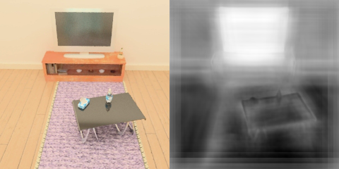
To split the features for each class, it is necessary to complete the feature extraction for semantic segmentation. Therefore, we define the features as the last convolution layer of the semantic segmentation networks. The channel of the features have the same dimension number as the class number. For instance, figure 3 shows the normalized features that are assigned to the TV class. The location and shape of the TV is obtained.

Furthermore, our discriminators minimize losses for each pixel, not for the whole input. The accuracy of semantic segmentation is decreased by local domain shift such as location of objects or contours of objects. Pixel-wise loss which uses local information for domain adaptation helps for local domain shift.

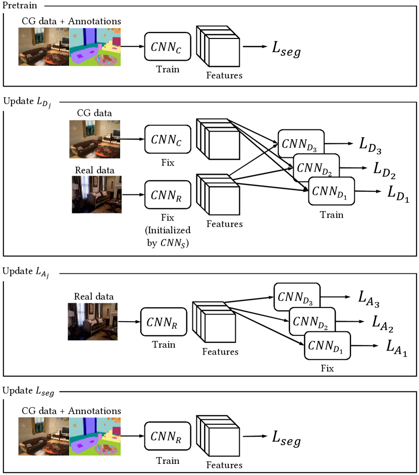
Figure 2 shows the training procedure. First, the $CNN_{C}$ is pre-trained by $L_{seg}$ which is the standard supervised semantic segmentation loss (2D Cross Entropy) with only computer graphics data. Then, the $CNN_{R}$ is initialized by $CNN_{C}$. Let ${L_{D}}_{j}$ be the domain loss of $j^{th}$ class and $p_{i}$ be the probability distribution for $i^{th}$ domain and $d_{i}$ be the one hot vector of ground truth labels and $k$ be the number of classes for semantic segmentation, and H be the height and W be the width of the output.

(1) $${L_{D}}_{j}=-\frac{1}{HW}\sum_{y=0}^{H}\sum_{x=0}^{W}\sum_{i=0}^{1}d_{i}\log p_{i}(x,y,j)$$

In the phase of updating ${L_{D}}_{j}$, computer graphics data are inputted to $CNN_{C}$ and real data are inputted to $CNN_{R}$ to obtain the features. The features are split along the channel and inputted to the discriminator ${CNN_{D}}_{j}$ for each class ${j}$. The weights of $CNN_{C}$ and $CNN_{R}$ are fixed and ${CNN_{D}}_{j}$ are iteratively updated by ${L_{D}}_{j}$. ${CNN_{D}}_{j}$ determines whether a given features have obtained from computer graphics data or real data. Domain labels are automatically assigned by data sources. For example, if the computer graphics data are inputted, the domain labels are assigned 0 and if the real data are inputted, the domain labels are assigned 1. No annotated image of semantic segmentation is required in this phase. Let ${L_{A}}_{j}$ be the adversarial loss of $j^{th}$ class.

(2) $${L_{A}}_{j}=-\frac{1}{HW}\sum_{y=0}^{H}\sum_{x=0}^{W}\sum_{i=0}^{1}(1-d_{i})\log p_{i}(x,y,j)$$

In the phase of updating ${L_{A}}_{j}$, real data are inputted to $CNN_{R}$ to obtain the features. The features are split along the channel and inputted to the discriminator ${CNN_{D}}_{j}$ for each class ${j}$. The weights of ${CNN_{D}}_{j}$ are fixed and $CNN_{R}$ is iteratively updated by ${L_{A}}_{j}$. Domain labels are inversed from the phase of updating ${L_{D}}_{j}$. For example, if the computer graphics domain is assigned 0 and the real domain is assigned 1 in the phase of updating ${L_{D}}_{j}$, the computer graphics domain is assigned 0 in this phase. No annotated image of semantic segmentation is required in this phase. By updating the adversarial loss, $CNN_{R}$ is trained to deceive ${CNN_{D}}_{j}$. $CNN_{R}$ is also updated by $L_{seg}$ with computer graphics data. Finally, $CNN_{R}$ and ${CNN_{D}}_{j}$ are iteratively updated by ${L_{D}}_{j}$, ${L_{A}}_{j}$ and $L_{seg}$.

Figure 2. The training procedure of class-wise adversarial adaptation. This figure shows an example of 3 classes for simplicity. $CNN_{C}$ and $CNN_{R}$ are the models for semantic segmentation. ${CNN_{D}}_{j}$ is a discriminator of $j^{th}$ class. Features are obtained from the last convolution layer of the models. First, $CNN_{C}$ is pre-trained with only computer graphics data. Then, $CNN_{R}$ and ${CNN_{D}}_{j}$ are iteratively updated by ${L_{D}}_{j}$, ${L_{A}}_{j}$ and $L_{seg}$.

Figure 3. The left shows the input rgb image and the right shows normalized features of TV. The place of TV tends to bright in the image.

3.2. Depth and Noise

Computer graphics can generate various modal for training inputs. Our experiments show that using depth modal increases accuracy. The depth image is concatenated with the rgb image on the fourth channel. At the inference phase, the depth image obtained by a depth sensor often lacks data. Therefore, we fill holes of depth image by using image inpainting algorithms (Bertalmio et al., 2001).

In general, computer graphics generate smooth images. However, the images taken by actual cameras have various noises. In order to bring rendered images closer to real images, we add synthetic noises to rendered images. Our synthetic noises are based on 2D image processing. Gaussian noise is added to the images as random pixel values according to the normal distribution. Salt and pepper noise randomly changes the pixels in the image to white or black. Gaussian blur and bilateral filter smooth images with kernel size of (9, 9). These noises are randomly applied for each input (including depth images) when training.

3.3. Architecture of Neural Networks

Our CNNs architecture for semantic segmentation is based on DenseNets (Huang et al., 2017) and PSPNets (Zhao et al., 2017). DenseNets is built from dense blocks. In each layer of dense block, feature maps of all preceding layers are concatenated. Therefore, it is easy to reuse the information from previous feature maps. The architecture fits for semantic segmentation where skip connections play an important role. Let $H_{l}$ be the function of a layer and $z_{l}$ be an input of $l^{th}$ layer:

(3) $$z_{l}=H_{l}([z_{0},z_{1},...,z_{l-1}])$$

where $[z_{0},z_{1},...,z_{l-1}]$ refers to the concatenation of the feature-maps produced in layers $0,...,l-1$. Let $M_{l}$ be the number of output feature maps and $r$ be the growth rate at $l^{th}$ layer in a denseblock. $M_{0}$ is determined by the output map size of the layer before the denseblock.

(4) $$M_{l}=M_{0}+rl$$

The dilated convolution also can integrate information of multiple receptive fields. The number of dilation is designed to become larger as the layer in the dense block gets deeper when downsampling phase. On the other hand, the number of dilation becomes smaller as the layer in the dense block gets deeper when upsampling phase. Table 1 shows our CNNs architecture for semantic segmentation. We define the Dilated Dense as a stack of dense layers with dilation. Each dense layer has two batchnormalizations (Ioffe and Szegedy, 2015), two ELU activation (Clevert et al., 2015) and two convolutions (kernel 1$\times$1 and 3$\times$3). PSPNets have a pyramid pool module. To improve performance of semantic segmentation, it is important to understand the contextual relationship and to integrate information from various size of receptive fields. For example, the contextual relationship means that a bottle is likely to be on a table. Pyramid pool module helps to understand the contextual relationship. We define the Pyramid Pool as five different scales of average pooling layers. After the Pyramid Pool, each output stream is concatenated. In addition, the strided convolution is used for the Upsample and the bilinear upsampling is used for the Downsample. The input size is 240$\times$240, and the number of channels depends on modal. In the case of using rgb and depth, they are concatenated and the number of channels becomes four.

We also use the Pyramid Pool for discriminators. Table 2 shows our CNNs architecture for discriminators. Before the first convolution, ReLU activation (Nair and Hinton, 2010) is applied for the features that are obtained from the last layer of semantic segmentation.

Table 1. CNNs architecture for semantic segmentation. The architecture is built with dense blocks, the pyramid pool module, dilated convolutions. We call it DensePyramid. The total number of convolutions is 84.

Block type	Output shape	No. of convs
7$\times$7 Conv	64$\times$240$\times$240	1
Average Pool	64$\times$120$\times$120	0
Dilated Dense (3 layers)	256$\times$120$\times$120	6
Downsample	128$\times$60$\times$60	1
Dilated Dense (6 layers)	512$\times$60$\times$60	12
Downsample	256$\times$30$\times$30	1
Dilated Dense (9 layers)	832$\times$30$\times$30	18
Pyramid Pool	832$\times$30$\times$30	5
Dilated Dense (9 layers)	1088$\times$30$\times$30	18
Upsample	272$\times$60$\times$60	1
Dilated Dense (6 layers)	656$\times$60$\times$60	12
Upsample	164$\times$120$\times$120	1
Dilated Dense (3 layers)	356$\times$120$\times$120	6
Bilinear upsampling	356$\times$240$\times$240	0
3$\times$3 Conv	256$\times$240$\times$240	1
1$\times$1 Conv	38$\times$240$\times$240	1

Table 2. CNNs architecture for discriminators. Our discriminator also has the pyramid pool module. After the final convolution layer, the ReLU function is applied as the activation function. We prepare the same number of discriminators as classes for class-wise adaptation.

Block type	Output shape	No. of convs
7$\times$7 Conv	16$\times$240$\times$240	1
Average Pool	16$\times$120$\times$120	0
7$\times$7 Conv	16$\times$120$\times$120	1
Average Pool	16$\times$60$\times$60	0
Pyramid Pool	16$\times$60$\times$60	4
Bilinear upsampling	16$\times$240$\times$240	0
1$\times$1 Conv	2$\times$240$\times$240	1

4. Computer Graphics Dataset

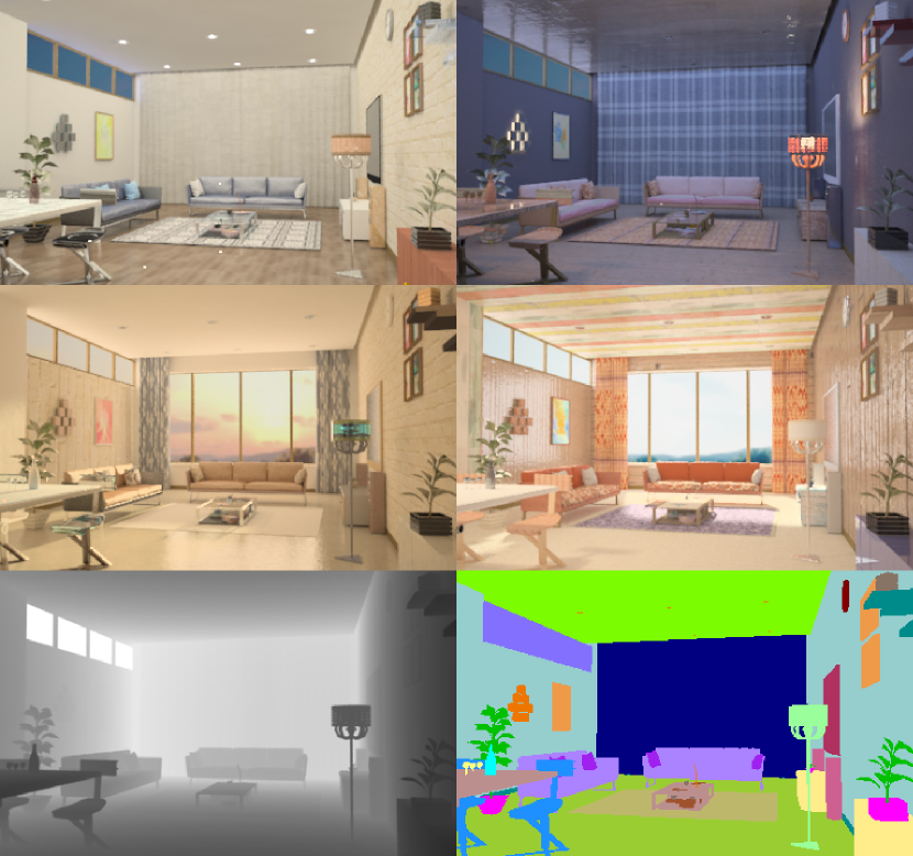
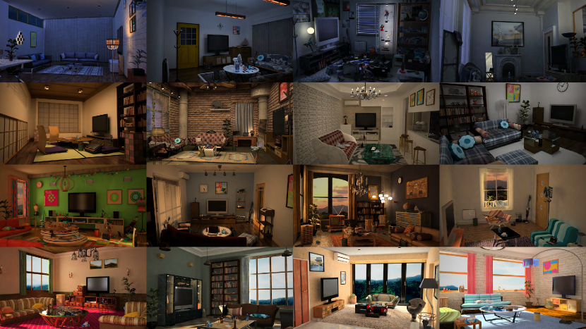
We have created 16 computer graphics rooms with different styles such as European, American and Asian. Each room has a different size, floor plan and objects. Unlike SUN CG (Song et al., 2017) etc., we prepared many kinds of props and put them on the rooms to bring closer to the actual rooms. Some classes for semantic segmentation have been added (plant, glass, cup, bottle, controller, dish, vase and clock) compared to SUN CG. We have to capture actual rooms to implement the mixed-reality application. In such applications, the interactions with several props are required, so our dataset is beneficial. We used Maya for modeling and V-Ray for rendering. Maya is a toolset to generate 3D computer graphics assets. V-ray is a renderer that provides photo-realistic rendering. All objects in rooms (excluding floor, door, wall and ceiling) are animated in MAYA. Furniture in each room are reallocated 5 times and perturbed by 20 frames at that time. Every room has 4 types of lighting conditions (morning, day, night with floor light and night with ceiling light). Therefore, a total of 400 variations of frames can be obtained for each room. In addition, the 4 types of materials change repeatedly every frame. As a result, various images can be rendered just by placing fixed cameras.

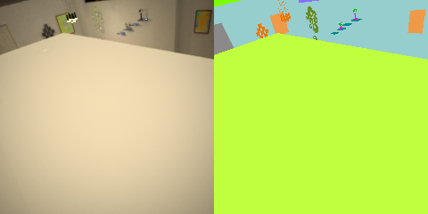
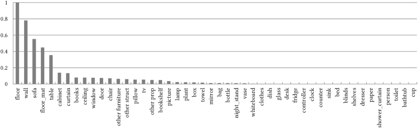
In semantic segmentation, the model is trained to understand contextual relationship. Thus, multiple objects should be included simultaneously in a single image as training data. As a bad case, if the whole image is filled with single color, the model may train the color as a specific object. Such a case is shown in Figure 5. Randomly placed cameras may generate such data. In our experiments, we first placed cameras randomly in rooms, but the model did not train well. Hence, we placed cameras on the circumference and each face to the center of the rooms. There are 16 cameras in each room on the circumference at a height of 90 cm and 180 cm. Our computer graphics can generate 102,400 different images (16 rooms, 400 frames and 16 cameras). In this work, 20K images which include rgb images, depth images, surface normal images and annotated images were rendered at 480$\times$640. At the training phase, we use data at 240$\times$240 and augment data by randomly cropping, changing gamma, and flipping etc.

Rendering took about 90 seconds for a single image. The CPU used for rendering is Intel Core i7-6800K. We show rendered images in Figure 4. The rendered images of other rooms are shown in Figure 8 and the statistics of annotated images are shown in Figure 9

Figure 4. Top left shows the rendered rgb image at night with ceiling light, top right shows the rendered rgb image at night with floor light, middle left shows the rendered rgb image at evening and middle right shows the rendered rgb image at morning. Each rendered rgb image has a different materials of furniture. Bottom left shows the rendered depth image and bottom right shows the rendered annotated image. The color of the annotated image means the object class.

Figure 5. The bad annotated image for training semantic segmentation. The left shows the rendered rgb image and the right shows the annotated. The field of view is almost filled with the bookshelf. The CNNs may train beige color as bookshelf.

5. Results

In this work, we use our computer graphics dataset for the source domain and SUN RGB-D for the target domain. SUN RGB-D dataset includes various indoor images of rgb and depth, so it is optimal for our task. First, we describe training conditions, the evaluation method and comparison with existing method in section 5.1. Then, we show the effect of depth and noise in 5.2. Finally, we present the effect of class-wise adaptation in 5.3.

5.1. Implementation Details

The model for semantic segmentation is trained for 96K iterations with a batch size of 40. The solver is Adam (Gopalan et al., 2011) with alpha = 1e-4, beta 1 = 0.9, and beta 2 = 0.999. The number of classes is 38, which is the same as SUN RGB-D, classes not used are assigned zero and not trained. We evaluate the validation data of SUN RGB-D. We report the evaluation results using pixel accuracy, mean pixel accuracy, and mean intersection over union (Long et al., 2015b), (Garcia-Garcia et al., 2017). Let $n_{ij}$ be the amount of pixels of class $i$ inferred to belong to class $j$ and $k$ be the number of classes. Pixel Accuracy (PA): the ratio between correctly predicted pixels and the total number of them.

(5) $$PA=\frac{\displaystyle\sum_{i=0}^{k}n_{ii}}{\displaystyle\sum_{i=0}^{k}\displaystyle\sum_{j=0}^{k}n_{ij}}$$

Mean Pixel Accuracy (MPA): the average over the total number of classes of class-wise pixel accuracy.

(6) $$MPA=\frac{1}{k+1}\displaystyle\sum_{i=0}^{k}\frac{n_{ii}}{\displaystyle\sum_{j=0}^{k}n_{ij}}$$

Mean Intersection over Union (MIoU): the ratio between the intersection and the union. These are calculated by ground truth pixels and predicted pixels.

(7) $$MIoU=\frac{1}{k+1}\displaystyle\sum_{i=0}^{k}\frac{n_{ii}}{\displaystyle\sum_{j=0}^{k}n_{ij}+\displaystyle\sum_{j=0}^{k}n_{ji}-n_{ii}}$$

Table 3 shows comparison of neural networks. DensePyramid is the architecture which was described in section 3.3. DensePyramid performs 2.1% higher in MIoU than SegNet. The models for domain adaptation are trained for 64K iterations with a batch size of 16. The solver is stochastic gradient descent (SGD) with learning rate = 1e-6.

Table 3. Comparison of neural networks. Models are trained with computer graphics data and evaluated with real data. The input modal is rgb.

Neural Networks	PA	MPA	MIoU
SegNet (Badrinarayanan et al., 2017)	0.470	0.377	0.105
DensePyramid	0.470	0.368	0.126

5.2. Effect of Depth and Noises

We can generate various modal by computer graphics. It is important to know which modal is most effective for domain shift between computer graphics data and real data. In this work, we compare rgb, depth and rgb + depth. The models are trained with only computer graphics data and evaluated with real data which are included in SUN RGB-D. We use DensePyramid as the models. The results are shown in Table 4. The model trained with rgb + depth performs 7.1% higher in PA than the model trained with rgb. The model trained with only depth also performs higher in PA and MPA, however rgb + depth is the best modal. The result shows that overfitting to color is avoided by using depth images.

We show the effect of synthetic noises in Table 4. We use rgb + depth modal and synthetic noises are added to both rgb and depth. Salt and pepper noise, gaussian noise, gaussian blur and bilateral filter are applied (see section 3.2). These noises are randomly added to input images at training time. The model with noises performs around 1% higher in PA, MPA and MIoU. Since real data have noises caused by cameras etc., synthetic noises work effectively in such an environment.

Table 4. Comparison of depth and noise. In the case of rgb + depth, the depth image is concatenated on the fourth channel of input.

Modal and Noise	PA	MPA	MIoU
rgb	0.470	0.368	0.126
depth	0.489	0.392	0.120
rgb + depth	0.543	0.436	0.137
rgb + depth + noise	0.552	0.444	0.149

5.3. Effect of Class-wise Adaptation

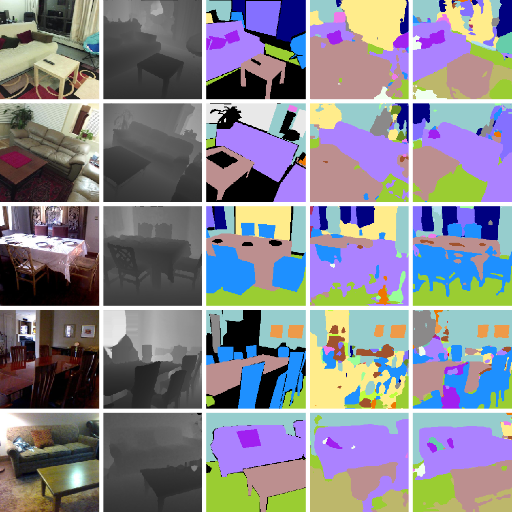
The result of class-wise adaptation is shown in Table 5. ”Adaptation” in Table 5 is a typical method that uses a single discriminator. The modal is rgb + depth, and synthetic noises are also added. The architecture of neural networks is DensePyramid. DensePyramid and the discriminators are trained with only computer graphics data and evaluated with real data which are included in SUN RGB-D. Our class-wise adaptation performs 2.3% higher in PA and 2.2% higher in MPA, and almost same in MIoU than ”no adaptation”. ”Adaptation” performs 1% higher only in MPA, and lower in MIoU. The experiment shows that our class-wise adaptation performs better than the typical method. Some results of sample images are shown in Figure 6. The baseline (no depth, no noise and no adaptation) often fails to parse boundaries of objects. For instance, the table and the floor are confused. Furthermore, the baseline does not parse chairs well. In contrast, our approach parses boundaries of objects well, such as tables, chairs and sofas. In addition, our approach parses chairs better than the baseline.

Table 5. Comparison of domain adaptation methods. Adaptation a typical method that uses a single discriminator.

Method	PA	MPA	MIoU
No Adaptation	0.552	0.444	0.149
Adaptation	0.555	0.452	0.138
Class-wise Adaptation	0.575	0.466	0.142

Figure 6. Qualitative results of semantic segmentation on the SUN RGB-D validation dataset. From the left column to the right column, input images, smoothed depth image, ground truth, outputs of baseline and outputs of our approach.

6. Application

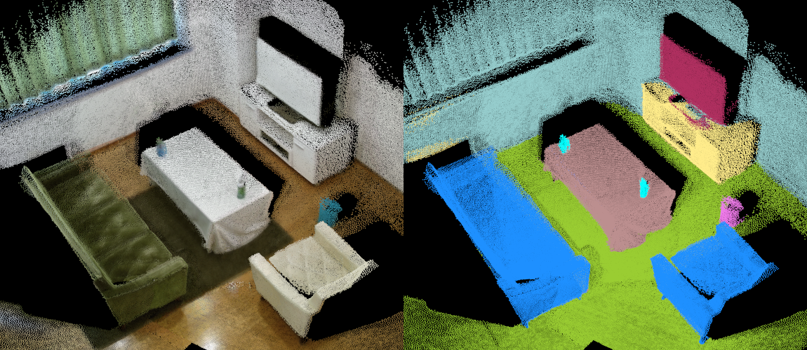
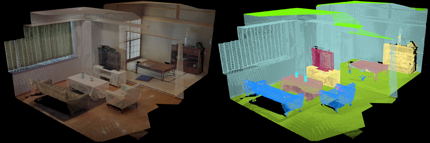
In this section, we introduce the 3D scene parsing application which is combined semantic segmentation with SLAM. As a first example, we use elastic fusion as SLAM (Whelan et al., 2015), (Whelan et al., 2016). The elastic fusion can reconstruct dense 3D space in real-time. The result is shown in Figure 1. The left shows actual rgb result and the right shows the parsing result. The scene is captured as point cloud format, and each color of the parsing result shows each object class. Since the frame by frame semantic segmentation is unstable, we vote latest several frames to obtain stable results. Hence, we got the accurate parsing result.

The whole system including semantic segmentation and SLAM run in 30fps with two NVIDIA Geforce GTX1080s. It takes less than 1 minute to parse a single room. Once the scene is captured and parsed, we can import the real scene into the virtual world and implement a mixed-reality application. For example, We can teleport to another world with your surroundings by vanishing only walls and change the background. Or, a real chair is replaced with a computer graphics chair and a virtual character sit on it. By using head mounted display, the more immersive experience can be realized.

Another example, we use matterport which is a 3D scanner for rooms. Matterport includes cameras and rotates to scan at the fixed position. We can obtain a whole room or building data by integrating the scanned results at several positions. In this work, we use point cloud format. We obtain the parsing results from virtual cameras, and back-project the results onto the point cloud. The result by matterport is shown in Figure 7. Although it is not in real-time, we can parse the objects with high accuracy by using matterport.

Figure 7. The 3D scene parsing result by using Matterport. The left shows actual rgb image and the right shows the parsing result. The scene is captured as point cloud format, and each color of the parsing result shows each object class.

7. Limitations and Future Work

Since we have not created human computer graphics models, our CNNs do not parse humans. Various rooms including various human computer graphics models should be prepared to parse humans, and we are currently preparing such data. Since human computer graphics models tend to differ from real humans, the adaptation is assumed to be more difficult. Therefore, we have to evaluate our approach on humans in the future.

In our data, all TVs are turned off. It may be necessary to randomly indicate some pictures on the synthetic TV to parse the real TV turned on. The challenge is how to distinguish between objects in the TV and real objects. We will tackle these problems as a future work.

The semantic segmentation becomes difficult when only a part of the object appears in the field of view. There is a possibility to solve that problem using time series data for training. Therefore, a faster rendering system such as a game engine is required to create time series data. However, since render quality and render time are a trade-off, we have to investigate whether our approach works with poor computer graphics dataset.

8. Conclusion

In this paper, we proposed the method that uses only computer graphics datasets to parse the real world 3D scenes. First, we presented the effectiveness of depth modal and synthetic noise for the domain shift. The depth image was concatenated with the rgb image on the fourth channel. Various synthetic noises based on 2D image processing were added to training data. Then, we developed the class-wise adaptation which can obtain domain invariant features. Our class-wise adaptation overcomes the domain shift between computer graphics and the real world without annotated real data. In addition, we created computer graphics rooms with a lot of props unlike the existing datasets. Our dataset is beneficial for the actual mixed-reality applications. Finally, we demonstrated the 3D scene parsing application which is combined semantic segmentation with SLAM. The latest several frames were voted to obtain stable results. We got the accurate parsing result in real-time on an actual room.

Figure 8. The rendered images of all 16 rooms with different conditions. $1^{st}$ row shows night with floor light, $2^{nd}$ row shows night with ceiling light, $3^{rd}$ row shows evening and $4^{th}$ row shows morning. Each room has different style, floor plan, furniture and density of objects.

Figure 9. The statistics of rendered annotated images of 20K. The ratio with floor labels is shown. Since we have created living room scenes, the items such as bed, shower curtain, toilet and bathtub are zero labels.

References

- (1)
- Badrinarayanan et al. (2017) Vijay Badrinarayanan, Ankur Handa, and Roberto Cipolla. 2017. SegNet: A Deep Convolutional Encoder-Decoder Architecture for Robust Semantic Pixel-Wise Labelling. The IEEE transactions on pattern analysis and machine intelligence (TPAMI) (2017).
- Bertalmio et al. (2001) Marcelo Bertalmio, Andrea L Bertozzi, and Guillermo Sapiro. 2001. Navier-stokes, fluid dynamics, and image and video inpainting. In Computer Vision and Pattern Recognition (CVPR), Proceedings of the 2001 IEEE Computer Society Conference on, Vol. 1. IEEE.
- Bousmalis et al. (2017) Konstantinos Bousmalis, Nathan Silberman, David Dohan, Dumitru Erhan, and Dilip Krishnan. 2017. Unsupervised Pixel-Level Domain Adaptation with Generative Adversarial Networks. The IEEE Conference on Computer Vision and Pattern Recognition (CVPR) (2017), 95–104.
- Chang et al. (2015) Angel X Chang, Thomas Funkhouser, Leonidas Guibas, Pat Hanrahan, Qixing Huang, Zimo Li, Silvio Savarese, Manolis Savva, Shuran Song, Hao Su, et al. 2015. ShapeNet: An Information-Rich 3D Model Repository. (2015). arXiv:arXiv:1512.03012
- Chen et al. (2016) Liang-Chieh Chen, George Papandreou, Iasonas Kokkinos, Kevin Murphy, and Alan L Yuille. 2016. Deeplab: Semantic image segmentation with deep convolutional nets, atrous convolution, and fully connected crfs. (2016). arXiv:arXiv:1606.00915
- Chen et al. (2015) Liang-Chieh Chen, George Papandreou, Iasonas Kokkinos, Kevin Murphy, and L. Alan Yuille. 2015. Semantic Image Segmentation with Deep Convolutional Nets and Fully Connected CRFs. In Proceedings of the International Conference on Learning Representations (ICLR).
- Clevert et al. (2015) Djork-Arné Clevert, Thomas Unterthiner, and Sepp Hochreiter. 2015. Fast and Accurate Deep Network Learning by Exponential Linear Units (ELUs). (2015). arXiv:arXiv:1511.07289
- Cordts et al. (2016) Marius Cordts, Mohamed Omran, Sebastian Ramos, Timo Rehfeld, Markus Enzweiler, Rodrigo Benenson, Uwe Franke, Stefan Roth, and Bernt Schiele. 2016. The Cityscapes Dataset for Semantic Urban Scene Understanding. In Proceedings of the IEEE Conference on Computer Vision and Pattern Recognition (CVPR).
- Everingham et al. (2015) Mark Everingham, S. M. Eslami, Luc Gool, Christopher K. Williams, John Winn, and Andrew Zisserman. 2015. The Pascal Visual Object Classes Challenge: A Retrospective. International Journal of Computer Vision 111, 1 (Jan. 2015), 98–136. https://doi.org/10.1007/s11263-014-0733-5
- Ganin and Lempitsky (2015) Yaroslav Ganin and Victor Lempitsky. 2015. Unsupervised domain adaptation by backpropagation. In Proceedings of the International Conference on Machine Learning (ICML). 1180–1189.
- Ganin et al. (2016) Yaroslav Ganin, Evgeniya Ustinova, Hana Ajakan, Pascal Germain, Hugo Larochelle, François Laviolette, Mario Marchand, and Victor Lempitsky. 2016. Domain-adversarial training of neural networks. Journal of Machine Learning Research 17, 59 (2016), 1–35.
- Garcia-Garcia et al. (2017) Alberto Garcia-Garcia, Sergio Orts-Escolano, Sergiu Oprea, Victor Villena-Martinez, and José García Rodríguez. 2017. A Review on Deep Learning Techniques Applied to Semantic Segmentation. (2017). arXiv:arXiv:1704.06857
- Goodfellow et al. (2014) Ian Goodfellow, Jean Pouget-Abadie, Mehdi Mirza, Bing Xu, David Warde-Farley, Sherjil Ozair, Aaron Courville, and Yoshua Bengio. 2014. Generative adversarial nets. In Proceedings of the Advances in neural information processing systems (NIPS). 2672–2680.
- Gopalan et al. (2011) Raghuraman Gopalan, Ruonan Li, and Rama Chellappa. 2011. Domain Adaptation for Object Recognition: An Unsupervised Approach. In Proceedings of the IEEE International Conference on Computer Vision (ICCV) (ICCV ’11). IEEE Computer Society, Washington, DC, USA, 999–1006. https://doi.org/10.1109/ICCV.2011.6126344
- Handa et al. (2015) Ankur Handa, Viorica Pătrăucean, Vijay Badrinarayanan, Simon Stent, and Roberto Cipolla. 2015. SceneNet: Understanding Real World Indoor Scenes With Synthetic Data. (2015). arXiv:arXiv:1511.07041
- He et al. (2016) Kaiming He, Xiangyu Zhang, Shaoqing Ren, and Jian Sun. 2016. Deep Residual Learning for Image Recognition. The IEEE Conference on Computer Vision and Pattern Recognition (CVPR) (2016), 770–778.
- Hoffman et al. (2016) Judy Hoffman, Dequan Wang, Fisher Yu, and Trevor Darrell. 2016. Fcns in the wild: Pixel-level adversarial and constraint-based adaptation. (2016). arXiv:arXiv:1612.02649
- Huang et al. (2017) Gao Huang, Zhuang Liu, Laurens van der Maaten, and Kilian Q Weinberger. 2017. Densely connected convolutional networks. In Proceedings of the IEEE Conference on Computer Vision and Pattern Recognition (CVPR).
- Ioffe and Szegedy (2015) Sergey Ioffe and Christian Szegedy. 2015. Batch Normalization: Accelerating Deep Network Training by Reducing Internal Covariate Shift. In Proceedings of the 32Nd International Conference on International Conference on Machine Learning - Volume 37 (ICML’15). JMLR.org, 448–456. http://dl.acm.org/citation.cfm?id=3045118.3045167
- Jakob (2010) Wenzel Jakob. 2010. Mitsuba renderer. (2010). http://www.mitsuba-renderer.org.
- Jégou et al. (2017) Simon Jégou, Michal Drozdzal, David Vazquez, Adriana Romero, and Yoshua Bengio. 2017. The one hundred layers tiramisu: Fully convolutional densenets for semantic segmentation. In Proceedings of the IEEE Computer Vision and Pattern Recognition Workshops (CVPRW), 2017 IEEE Conference on. 1175–1183.
- Kanazawa et al. (2017) Angjoo Kanazawa, Michael J. Black, David W. Jacobs, and Jitendra Malik. 2017. End-to-end Recovery of Human Shape and Pose. arXiv (2017).
- Lin et al. (2014) Tsung-Yi Lin, Michael Maire, Serge Belongie, James Hays, Pietro Perona, Deva Ramanan, Piotr Dollár, and C. Lawrence Zitnick. 2014. Microsoft COCO: Common Objects in Context. Springer International Publishing, Cham, 740–755. https://doi.org/10.1007/978-3-319-10602-1_48
- Liu and Tuzel (2016) Ming-Yu Liu and Oncel Tuzel. 2016. Coupled generative adversarial networks. In Proceedings of the Advances in neural information processing systems (NIPS). 469–477.
- Long et al. (2015b) Jonathan Long, Evan Shelhamer, and Trevor Darrell. 2015b. Fully Convolutional Networks for Semantic Segmentation. In Proceedings of the IEEE Conference on Computer Vision and Pattern Recognition (CVPR). 3431–3440.
- Long et al. (2015a) Mingsheng Long, Yue Cao, Jianmin Wang, and Michael I. Jordan. 2015a. Learning Transferable Features with Deep Adaptation Networks. In Proceedings of the International Conference on Machine Learning (ICML). 97–105.
- Long et al. (2016) Mingsheng Long, Han Zhu, Jianmin Wang, and Michael I Jordan. 2016. Unsupervised domain adaptation with residual transfer networks. In Proceedings of the Advances in Neural Information Processing Systems (NIPS). 136–144.
- McCormac et al. (2017) John McCormac, Ankur Handa, Stefan Leutenegger, and Andrew J Davison. 2017. SceneNet RGB-D: Can 5M Synthetic Images Beat Generic ImageNet Pre-training on Indoor Segmentation? The IEEE International Conference on Computer Vision (ICCV) 1 (2017), 2697–2706.
- Nair and Hinton (2010) Vinod Nair and Geoffrey E. Hinton. 2010. Rectified Linear Units Improve Restricted Boltzmann Machines. In Proceedings of the 27th International Conference on International Conference on Machine Learning (ICML’10). Omnipress, USA, 807–814. http://dl.acm.org/citation.cfm?id=3104322.3104425
- Noh et al. (2015) Hyeonwoo Noh, Seunghoon Hong, and Bohyung Han. 2015. Learning Deconvolution Network for Semantic Segmentation. In Proceedings of the IEEE International Conference on Computer Vision (CVPR). 1520–1528.
- Pedersen (2013) S. A. Pedersen. 2013. Progressive photon mapping on gpus. Master’s thesis. Norwegian University of Science and Technology.
- Qiu and Yuille (2016) Weichao Qiu and Alan Yuille. 2016. UnrealCV: Connecting Computer Vision to Unreal Engine. Springer International Publishing, Cham, 909–916. https://doi.org/10.1007/978-3-319-49409-8_75
- Richter et al. (2017) Stephan R. Richter, Zeeshan Hayder, and Vladlen Koltun. 2017. Playing for Benchmarks. In Proceedings of the IEEE International Conference on Computer Vision (ICCV).
- Saenko et al. (2010) Kate Saenko, Brian Kulis, Mario Fritz, and Trevor Darrell. 2010. Adapting Visual Category Models to New Domains. Springer Berlin Heidelberg, Berlin, Heidelberg, 213–226. https://doi.org/10.1007/978-3-642-15561-1_16
- Sankaranarayanan et al. (2017) Swami Sankaranarayanan, Yogesh Balaji, Arpit Jain, Ser Nam Lim, and Rama Chellappa. 2017. Unsupervised Domain Adaptation for Semantic Segmentation with GANs. (2017). arXiv:arXiv:1711.06969
- Song et al. (2015) Shuran Song, Samuel P. Lichtenberg, and Jianxiong Xiao. 2015. SUN RGB-D: A RGB-D Scene Understanding Benchmark Suite. In Proceedings of the IEEE Conference on Computer Vision and Pattern Recognition (CVPR).
- Song et al. (2017) Shuran Song, Fisher Yu, Andy Zeng, Angel X Chang, Manolis Savva, and Thomas Funkhouser. 2017. Semantic Scene Completion from a Single Depth Image. (2017).
- Sun and Saenko (2014) Baochen Sun and Kate Saenko. 2014. From Virtual to Reality: Fast Adaptation of Virtual Object Detectors to Real Domains. In Proceedings of the British Machine Vision Conference. BMVA Press. https://doi.org/10.5244/C.28.82
- Tzeng et al. (2015) Eric Tzeng, Judy Hoffman, Trevor Darrell, and Kate Saenko. 2015. Simultaneous Deep Transfer Across Domains and Tasks. In Proceedings of the IEEE International Conference in Computer Vision (ICCV).
- Tzeng et al. (2017) Eric Tzeng, Judy Hoffman, Kate Saenko, and Trevor Darrell. 2017. Adversarial Discriminative Domain Adaptation. In Proceedings of the IEEE Conference on Computer Vision and Pattern Recognition (CVPR). 2962–2971.
- Whelan et al. (2015) T Whelan, S Leutenegger, RF Salas-Moreno, B Glocker, and AJ Davison. 2015. ElasticFusion: Dense SLAM without a pose graph. https://doi.org/10.15607/RSS.2015.XI.001
- Whelan et al. (2016) Thomas Whelan, Renato F Salas-Moreno, Ben Glocker, Andrew J Davison, and Stefan Leutenegger. 2016. ElasticFusion: Real-time dense SLAM and light source estimation. The International Journal of Robotics Research 35, 14 (2016), 1697–1716. https://doi.org/10.1177/0278364916669237 arXiv:https://doi.org/10.1177/0278364916669237
- Wu et al. (2016) Zifeng Wu, Chunhua Shen, and Anton van den Hengel. 2016. Wider or Deeper: Revisiting the ResNet Model for Visual Recognition. (2016). arXiv:arXiv:1611.10080
- Wu et al. (2015) Zhirong Wu, Shuran Song, Aditya Khosla, Fisher Yu, Linguang Zhang, Xiaoou Tang, and Jianxiong Xiao. 2015. 3D ShapeNets: A Deep Representation for Volumetric Shapes. In Proceedings of the IEEE Conference on Computer Vision and Pattern Recognition (CVPR). 1912–1920.
- Yu and Koltun (2016) Fisher Yu and Vladlen Koltun. 2016. Multi-Scale Context Aggregation by Dilated Convolutions. In Proceedings of the International Conference on Learning Representations (ICLR).
- Zhang et al. (2017a) Yang Zhang, Philip David, and Boqing Gong. 2017a. Curriculum Domain Adaptation for Semantic Segmentation of Urban Scenes. In Proceedings of the IEEE International Conference on Computer Vision (ICCV).
- Zhang et al. (2017b) Yinda Zhang, Shuran Song, Ersin Yumer, Manolis Savva, Joon-Young Lee, Hailin Jin, and Thomas Funkhouser. 2017b. Physically-Based Rendering for Indoor Scene Understanding Using Convolutional Neural Networks. The IEEE Conference on Computer Vision and Pattern Recognition (CVPR) (2017).
- Zhao et al. (2017) Hengshuang Zhao, Jianping Shi, Xiaojuan Qi, Xiaogang Wang, and Jiaya Jia. 2017. Pyramid Scene Parsing Network. In Proceedings of the IEEE Conference on Computer Vision and Pattern Recognition (CVPR).
- Zheng et al. (2015) Shuai Zheng, Sadeep Jayasumana, Bernardino Romera-Paredes, Vibhav Vineet, Zhizhong Su, Dalong Du, Chang Huang, and Philip H. S. Torr. 2015. Conditional Random Fields as Recurrent Neural Networks. In Proceedings of the IEEE International Conference on Computer Vision (CVPR). 1529–1537.
- Zhu et al. (2017) Jun-Yan Zhu, Taesung Park, Phillip Isola, and Alexei A. Efros. 2017. Unpaired Image-To-Image Translation Using Cycle-Consistent Adversarial Networks. In Proceedings of the IEEE International Conference on Computer Vision (ICCV).