Instanton based importance sampling for rare events in stochastic PDEs

Abstract

We present a new method for sampling rare and large fluctuations in a non-equilibrium system governed by a stochastic partial differential equation (SPDE) with additive forcing. To this end, we deploy the so-called instanton formalism that corresponds to a saddle-point approximation of the action in the path integral formulation of the underlying SPDE. The crucial step in our approach is the formulation of an alternative SPDE that incorporates knowledge of the instanton solution such that we are able to constrain the dynamical evolutions around extreme flow configurations only. Finally, a reweighting procedure based on the Girsanov theorem is applied to recover the full distribution function of the original system. The entire procedure is demonstrated on the example of the one-dimensional Burgers equation. Furthermore, we compare our method to conventional direct numerical simulations as well as to Hybrid Monte Carlo methods. It will be shown that the instanton-based sampling method outperforms both approaches and allows for an accurate quantification of the whole probability density function of velocity gradients from the core to the very far tails.

I Introduction

Non-equilibrium systems that possess a large number of interacting degrees of freedom typically exhibit strongly anomalous statistical properties which can be attributed to rare large fluctuations. Typical examples include the occurrence rate of earthquakes Knopoff and Kagan (1977), the existence of rogue waves Onorato et al. (2013); Dematteis, Grafke, and Vanden-Eijnden (2018); Hadjihosseini et al. (2016), crashes in the stock market Ghashghaie et al. (1996); Longin (2016); Bouchaud and Potters (2009), the occurrence of epileptic seizures Lehnertz (2006), or perhaps the most enigmatic case, the distribution of velocity increments in hydrodynamic turbulence Frisch (1995). In turbulence theory, a central notion is the energy cascade which implies a non-linear and chaotic transfer between different scales Alexakis and Biferale (2018). Although well-established descriptions by Richardson, Kolmogorov, Onsager, Heisenberg, and others (see the reviews Frisch (1995); Monin and Yaglom (2007)) can capture the mean field features of the cascade process in a phenomenological way, the nature of small-scale turbulent energy dissipation is far less understood and is usually attributed to nearly singular localized vortical structures Yeung, Zhai, and Sreenivasan (2015); Debue et al. (2018). Empirically, the energy transfer from large to small scales is accompanied by a breaking of self-similarity of the probability density function (PDF) of velocity increments, a phenomenon called intermittency. Intermittency is intimately connected to non-Gaussian statistics and extreme events and is often described in a statistical sense, using random multiplicative cascades leading to multifractal measures Frisch (1995); Benzi and Biferale (2009). On the other hand, it manifests itself by the presence of singular or quasi-singular structures, highly concentrated in a few spatial locations. From a mathematical point of view, large fluctuations of the fluid variables are controlled by the theory of large deviations Freidlin and Wentzell (1984); Varadhan (2016); Touchette (2009); Cecconi et al. (2014), which is concerned with the exponential decay of the PDF for large field values, see, e.g., the paper(Bouchet, Laurie, and Zaboronski, 2014) for a numerical application based on the Onsager-Machlup functional in the context of geophysical flows.

Besides numerical large deviation methods, cloning and selection strategies (that favor the desired event) have evolved into mature simulation techniques, too Grassberger (2002); Giardina et al. (2011). Recently, such methods have been deployed in order to investigate return times in Ornstein-Uhlenbeck processes, in the drag forces acting on an object in turbulent flows Lestang et al. (2018), as well as for extreme heat waves in weather dynamics Ragone, Wouters, and Bouchet (2018). Other numerical methods include direct importance sampling in configuration space Dellago et al. (1998), a modification of transition path methods Touchette (2009) in form of the so-called string method Weinan, Ren, and Vanden-Eijnden (2002) and the geometric minimum action methodHeymann and Vanden-Eijnden (2008).

In this paper we are interested to apply saddle point techniques to estimate extreme events (also called instantons or optimal fluctuations) as originally introduced in the context of solid state disordered systems Lifshitz (1964); Halperin and Lax (1966); Zittartz and Langer (1966); Langer (1967, 1969) (see also Grafke, Grauer, and Schäfer (2015) for an overview). Especially, we refer to the works of Zittartz and Langer Zittartz and Langer (1966); Langer (1967, 1969) which contain nearly all the recipes we are using today. Single- and multi-instantons dynamics have often been advocated as some of the possible mechanisms of anomalous fluctuations in hydrodynamical systems and models thereof  Balkovsky et al. (1996, 1997); De Pietro, Mailybaev, and Biferale (2017); Mailybaev (2013); Daumont, Dombre, and Gilson (2000). We will use the so-called Janssen-de Dominicis Janssen (1976); De Dominicis (1976) path integral formulation of the Martin-Siggia-Rose (MSR) operator technique  Martin, Siggia, and Rose (1973) for classical stochastic systems. In particular, we will apply it to the important case of the one-dimensional stochastically forced Burgers equation:

$$u_{t}(x,t)+u(x,t)u_{x}(x,t)=\nu u_{xx}(x,t)+\eta(x,t)\;,$$ (1)

where the nonlinearity tends to form shock fronts that are ultimately smeared out by viscosity and lead to the appearance of large negative velocity gradients (see below for further details on the equations). The Burgers equation constitutes a high-dimensional and highly non-trivial example of a complex system with fluctuations far away from Gaussianity. The Burgers equation can be also considered as a simplified one-dimensional compressible version of the Navier-Stokes equation and has been extensively studied in the past decades Gotoh (1994); Chekhlov and Yakhot (1995a, b); Bouchaud, Mezard, and Parisi (1995); Gurarie and Migdal (1996); Balkovsky et al. (1996, 1997); Falkovich et al. (1996); Polyakov (1995); Boldyrev (1997); E et al. (2000); E and Vanden Eijnden (2000, 1999); Friedrich et al. (2018) (see also the review Bec and Khanin (2007)) using numerical simulations Chekhlov and Yakhot (1995a, b); Gotoh (1994), the replica method Bouchaud, Mezard, and Parisi (1995), operator product expansion Polyakov (1995); Boldyrev (1997); Lässig (2000); Friedrich et al. (2018), asymptotic methods E et al. (2000); E and Vanden Eijnden (2000, 1999) as well as instanton methods Gurarie and Migdal (1996); Balkovsky et al. (1996, 1997); Falkovich et al. (1996); Grafke, Grauer, and Schäfer (2015). Similarly, the Kardar-Parisi-Zhang equation, which is strictly connected to (1), has also recently been studied using instantons  Janas, Kamenev, and Meerson (2016); Smith, Kamenev, and Meerson (2018).

The main problem when dealing with instanton approximations of the whole probability distribution is to evaluate the fluctuations around them, which is, in turn, connected to the most important problem of quantifying the influence of the saddle-point solution to all field values, including the ones that are not extremal.

In this paper, we propose a new method to study the shape of the PDF of the Burgers velocity gradients $u_{x}$, in those parameter regions where it is dominated by instantons, considering also the fluctuations around the saddle point configurations. To do that, we will decompose the velocity field in the MSR action into a contribution that stems from the instanton as well as a fluctuation around this object. We then proceed and derive an evolution equation for the fluctuation in the background of the instanton solution for a given gradient. A subsequent reweighting procedure allows us to calculate the full PDF with a much more accurate description of the tails in comparison to ordinary direct numerical simulations (DNS) of Burgers turbulence. We also show that our method is computationally less substantially challenging than other approaches based on Markov Chain Monte Carlo methods to generate extreme and rare flow configurations Margazoglou et al. (2018). Hence, the method can be considered as an optimal application of rare events importance sampling and we call it the Instanton based Importance Sampling (IbIS), see also the work Bühler (2007) for a similar idea. In our formulation, the method is general enough to be applied to many different SPDEs.

The paper is organized as follows: In section II we review the path integral formulation of stochastic systems. Section III constitutes the core of the paper, where we present our reweighting procedure. In section IV we describe in detail the numerical protocol and we compare the results obtained with IbIS against those obtained using DNS and a Hybrid Monte Carlo approach Margazoglou et al. (2018). We close with a summary and an outlook on further applications.

II Path integral formulation and instantons

To make our exposition self-consistent, here we describe the path integral formulation of stochastic systems, the subsequent derivation of the instanton equations, and the calculation of fluctuations around the instanton using an appropriate reweighting procedure. The presentation follows closely the seminal work of Balkovsky et al. (1996).

II.1 Path integral formulation of stochastic systems

The Martin-Siggia-Rose-Janssen-de Dominicis formalism (hereinafter referred to as MSRJD formalism) Martin, Siggia, and Rose (1973); Janssen (1976); De Dominicis (1976) was developed in the early 1970’s to calculate statistical properties of classical systems using a path integral formulation. Following the same notation as inChernykh and Stepanov (2001); Grafke, Grauer, and Schäfer (2015), we consider a stochastic differential equation

$$\dot{u}+N[u,x]=\eta(x,t)\ ,$$ (2)

where $\eta$ is an additive Gaussian noise with correlation

$$\langle\eta(x,t)\eta(x+r,t+s)\rangle=\chi(r)\delta(s)\ .$$ (3)

Here, the $\delta$-correlation implies that the forcing $\eta$ is white in time, while $\chi(r)$ is some arbitrary spatial correlation. Considering that from Eq. (2) the field $u$ is a functional $u[\eta]$ of the forcing $\eta$, we introduce the MSRJD formalism as follows. The expectation value of an observable $\left<\mathcal{O}[u]\right>$, as the average over all possible noise realizations, can be defined as

$$\langle\mathcal{O}[u]\rangle=\int\mathcal{D}\eta\,\mathcal{O}[u[\eta]]\,e^{-\int dt\,\langle\eta,\chi^{-1}\eta\rangle/2}\ ,$$ (4)

where the integral in the exponent derives from $\eta$ being normally distributed, with $\langle\ \cdot\ ,\ \cdot\ \rangle$ being the $L^{2}$ inner product. Changing the integration from $\eta$ to $u$, given Eq. (2), modifies the measure in Eq. (4) as $\mathcal{D}\eta=J[u]\,\mathcal{D}u$, where $J[u]=\mathrm{det}\left(\frac{\delta\eta}{\delta u}\right)=\mathrm{det}\left(\partial_{t}+\frac{\delta N}{\delta u}\right)$ is the Jacobian associated to the map $\eta\mapsto u$. This results into what is called the Onsager-Machlup functionalOnsager and Machlup (1953)

$$\langle\mathcal{O}[u]\rangle=\int\mathcal{D}u\,\mathcal{O}[u]J[u]\,e^{-\int dt\,\langle\dot{u}+N[u],\chi^{-1}(\dot{u}+N[u])\rangle/2}\ .$$ (5)

It is the starting point for direct minimization of the Lagrangian action

$$S_{\mathcal{L}}[u,\dot{u}]=\frac{1}{2}\int dt\,\langle\dot{u}+N[u],\chi^{-1}(\dot{u}+N[u])\rangle\ .$$ (6)

Most of the time, it is more convenient to work with the original correlation function $\chi$ instead of its inverse. We therefore perform a Hubbard-Stratonovich transformation, which introduces an auxiliary field $\tilde{p}$ and by virtue of a Fourier transform and completing the square eliminates the inverse of the correlation function $\chi^{-1}$ and in addition the noise appears only linearly in the action:

$$\langle\mathcal{O}[u]\rangle=\int\mathcal{D}\eta\mathcal{D}\tilde{p}\,\mathcal{O}[u[\eta]]\,e^{-\int dt\,[\langle\tilde{p},\chi\tilde{p}\rangle/2-\mathbbm{i}\langle\tilde{p},\eta\rangle]}\ .$$ (7)

We then execute the coordinate transformation from $\eta$ to $u$

$$\langle\mathcal{O}[u]\rangle=\int\mathcal{D}u\mathcal{D}\tilde{p}\,\mathcal{O}[u]J[u]\,e^{-S[u,\tilde{p}]},$$ (8)

with the action function $S[u,\tilde{p}]$ given by

$$S[u,\tilde{p}]=\int dt\,\left[-\mathbbm{i}\langle\tilde{p},\dot{u}+N[u]\rangle+\frac{1}{2}\langle\tilde{p},\chi\tilde{p}\rangle\right]\ .$$

For the purpose of convenience to obtain an Euclidian path integral we now substitute $\tilde{p}$ with $p$, by use of the relation $\tilde{p}=\mathbbm{i}\,p$ and obtain the Hamiltonian action

$$S_{\mathcal{H}}[u,p]=\int dt\,\left[\langle p,\dot{u}+N[u]\rangle-\frac{1}{2}\langle p,\chi p\rangle\right]\ .$$ (9)

The next step is to minimize this action functional to obtain the instanton solutions.

II.2 Instantons

We are interested in rare and large fluctuations of velocity gradients $u_{x}(x,t)$ in the Burgers equation (1). Since this chaotic and turbulent system is invariant under time translations and Galilean transformations, the probability function of velocity gradients can be cast into the following form as a path integral

$$\mathcal{P}(a) =\langle\delta(u_{x}(0,0)-a)\rangle$$

$$=\int\mathcal{D}u\,\mathcal{D}p\,\int_{-\mathbbm{i}\infty}^{\mathbbm{i}\infty}d\mathcal{F}\,\mathrm{exp}\{-S_{\mathcal{H}}+\mathcal{F}\,[u_{x}(0,0)-a]\}\ .$$ (10)

Here $\mathcal{F}$ stems from the Fourier transformat of the $\delta$-function and serves as a Lagrange multiplier. Hence, from Eq. (9) we have

$$S_{\mathcal{H}}[u,p]=\ \int_{-\infty}^{0}dt\,\int dx\,p(x,t)\,(u_{t}+uu_{x}-\nu u_{xx})$$

$$-\frac{1}{2}\int_{-\infty}^{0}dt\,\int dx\,dx^{\prime}\,p(x,t)\chi(x-x^{\prime})p(x^{\prime},t)\ .$$ (11)

Now $\mathcal{F}$ is treated as a large parameter so that the saddle point approximation can be used in order to derive instanton configurations, i.e. “classical” solutions that minimize the action and therefore dominate the path integral of Eq. (II.2). The instanton equations are obtained from the conditions

$$\frac{\delta S}{\delta u}=0\quad\text{and}\quad\frac{\delta S}{\delta p}=0\ .$$ (12)

When carried out, the functional derivatives above yield the so called instanton equations:

$$u_{t}+uu_{x}-\nu u_{xx}=\chi*p\,,$$ (13)

$$p_{t}+up_{x}+\nu p_{xx}=\mathcal{F}\,\delta(t)\,\delta^{\prime}(x)\,,$$ (14)

where $u(x,t)$ and $p(x,t)$ have the following boundary conditions:

$$\ \underset{t\rightarrow-\infty}{\mathrm{lim}}\ u(x,t)=0\qquad\ \ \underset{t\rightarrow-\infty}{\mathrm{lim}}\ p(x,t)=0$$

$$\underset{|x|\rightarrow+\infty}{\mathrm{lim}}\ u(x,t)=0\qquad\underset{|x|\rightarrow+\infty}{\mathrm{lim}}\ p(x,t)=0$$

and $\chi*p$ is the convolution

$$(\chi*p)(x)=\int dx^{\prime}\,\chi(x-x^{\prime})\,p(x^{\prime},t)\ .$$ (15)

Because of the $\delta$-function, the RHS of Eq. (14) is an initial condition for $p$. Furthermore, the RHS of Eq. (13) will often be abbreviated:

$$\chi*p=P\ .$$ (16)

Making use of Eqs. (II.2) and (13) we may calculate the instanton action

$$S^{I(a)}=\frac{1}{2}\,\int_{-\infty}^{0}dt\,\int dx\,dx^{\prime}\,p(x,t)\,\chi(x-x^{\prime})\,p(x^{\prime},t)\ ,$$ (17)

where $I(a)$ denotes that the instanton has a gradient of $u_{x}=a$. We denote all other instanton related quantities in a similar way.

III Instanton based Reweighting

The process of reweighting allows us to assemble the PDF related to the stochastic Burgers equation by solving the stochastic PDE for the fluctuations around the instanton. In order to derive the instanton equations, we considered the minimum of the Janssen-de Dominicis action $S_{\mathcal{H}}[u,p]$. However, to derive this stochastic PDE, we will work again with the original Onsager-Machlup action (see Eq. (6)):

$$S_{\mathcal{L}}[u,\dot{u}] =\frac{1}{2}\int dt\,\langle\dot{u}+N[u],\chi^{-1}(\dot{u}+N[u])\rangle$$

$$=\frac{1}{2}\int dt\,dx\,dx^{\prime}\,\left[u_{t}+uu_{x}-\nu u_{xx}\right]$$ (18)

$$\qquad\times\,\chi^{-1}(x-x^{\prime})\,\left[u_{t}+uu_{x^{\prime}}+\nu u_{x^{\prime}x^{\prime}}\right].$$

We then decompose the field into instanton and fluctuation

$$u=u^{I(a)}+\delta u\ .$$ (19)

This results in

$$S_{\mathcal{L}} =\frac{1}{2}\int dt\,dx\,dx^{\prime}\,\Big{[}P^{I(a)}+\delta u_{t}+\delta u\delta u_{x}-\nu\delta u_{xx}$$

$$\qquad+(u^{I(a)}\delta u)_{x}\Big{]}\,\chi^{-1}(x-x^{\prime})\,[\mathellipsis]$$

$$=S^{I(a)}+\tilde{S}^{a}-\frac{1}{2}\int dt\,dx\,p^{I(a)}_{x}(\delta u)^{2}\ ,$$ (20)

with

$$\tilde{S}^{a}=\frac{1}{2}\int dt\,dx\,dx^{\prime}\, [\delta u_{t}+\delta u\delta u_{x}-\nu\delta u_{xx}+(u^{I(a)}\delta u)_{x}]\,$$

$$\qquad\times\chi^{-1}(x-x^{\prime})\,[\mathellipsis]\ .$$ (21)

Here $[\mathellipsis]$ denotes the appropriate expression evaluated at the position $x^{\prime}$. Note that all linear variations vanish by definition of the instanton. Thus we define

$$\Delta S^{a}=S_{\mathcal{L}}-\tilde{S}^{a}=S^{I(a)}-\frac{1}{2}\int dt\,dx\,p^{I(a)}_{x}(\delta u)^{2}\ .$$ (22)

Now to derive the stochastic equation corresponding to the action $\tilde{S}^{a}$, we reverse the derivation of the path integral formulation and obtain

$$\delta u_{t}+\delta u\delta u_{x}-\nu\delta u_{xx}=\eta-(u^{I(a)}\delta u)_{x}\ .$$ (23)

Next, we have to change the path measure for this process in order to connect the statistics to the original one. To do that, we first consider the identity

$$P_{S_{\mathcal{L}}}(s) :=\delta(u_{x}(0,0)-s)e^{-S_{\mathcal{L}}}$$

$$=\delta(u_{x}(0,0)-s)e^{-(\tilde{S}^{a}+\Delta S^{a})}$$

$$=\delta(\delta u_{x}(0,0)+a-s)e^{-\tilde{S}^{a}}e^{-\Delta S^{a}},$$ (24)

where $P_{S_{\mathcal{L}}}(s)$ denotes the path measure of the distribution of gradients, $s=u_{x}(x,t)$ at $(x,t)=(0,0)$ in the original Burgers equation as one would obtain it by performing numerical simulations of (1). On the other hand, if we sample events for the gradient of the fluctuations, $\delta u$, around the instanton $I^{(a)}$, i.e. when $u_{x}=a$ through the new stochastic equation (23) we would get a PDF generated by the measure $e^{-\tilde{S}^{a}}$. The last equality in (24) tell us that in order to get the unbiased original PDF we need to reweight with a factor $e^{-\Delta{S}^{a}}$. A similar approach was formulated in a simpler setting by Bühler (2007).

If we would proceed in choosing one value $u_{x}=a$ to calculate the instanton with $u_{x}^{I(a)}(x=0,t=0)=a$, we will be able to sample the statistics near this value very efficiently. However, values $u_{x}=s$ far away from $a$ will be sampled with poor performance. Thus a major step is to choose $s=a$, which means that for every point $u_{x}=a$ in the PDF we first calculate the instanton and then using Eq. (22) obtain the PDF at $u_{x}=a$. This procedure is further motivated in Fig. 1. This figure shows the PDFs for the gradient of the fluctuations $\delta u_{x}(0,0)$ around the instanton $u^{I(a)}$, measured at (0,0) and shifted by $a$ (for comparison) using six different values of $u_{x}=a$, obtained from simulations of Eq. (23). Thus the actual form of the Girsanov transformation used in our instanton reweighting approach reads

$$P_{S_{\mathcal{L}}}(s) :=\delta(u_{x}(0,0)-s)e^{-S_{\mathcal{L}}}$$

$$=\delta(\delta u_{x}(0,0))e^{-(\tilde{S}^{a}+\Delta S^{a})}$$ (25)

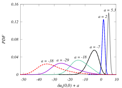
Figure 1: Shape of the PDFs for the gradient of the fluctuations $\delta u_{x}$ (shifted by $a$) around the instanton $u^{I(a)}$ for six different values of $u_{x}=a$.

IV Numerical simulations of rare events

In this section we describe the numerical procedure to calculate the full PDF of velocity gradients step by step. The numerical integration of the stochastic PDE given in Eq. (23)

$$\delta u_{t}+\delta u\delta u_{x}-\nu\delta u_{xx}=\eta-(u^{I(a)}\delta u)_{x}\$$

is achieved using the Euler-Maruyama method Higham. (2001) in combination with an integrating factor Canuto et al. (1988) for the dissipative term. The spatial correlation function of the forcing (3) follows a power law proportional to $k^{-3}$ in Fourier space and has a cutoff at $k_{F}=N_{x}/3$, where $N_{x}$ is the spatial number of grid points. The nonlinear term is evaluated with the pseudospectral method. The instanton equations (13)-(14) are solved using an iterative method as described in Chernykh and Stepanov Chernykh and Stepanov (2001); Grafke, Grauer, and Schäfer (2015).

Results of an instanton configuration for a certain gradient $u_{x}^{I(a)}(x=0,t=0)=a$, and a snapshot of a typical realization of Eq. (23) $\delta u$ added with $u^{I(a)}$ are displayed in Fig. 2.

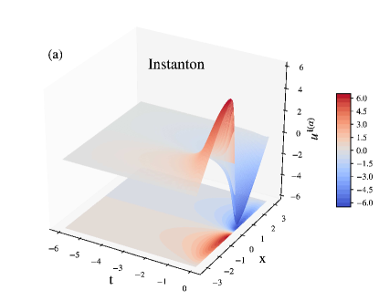
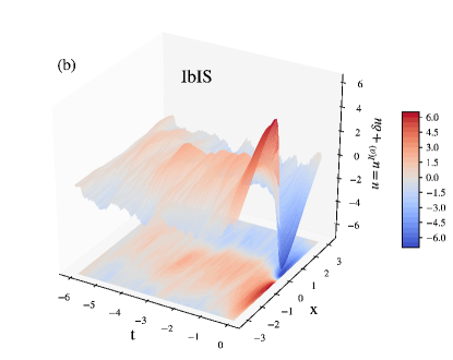
Figure 2: (a) Instanton solution $u^{I(a)}$ for $N_{x}=64$, $N_{t}=576$, $\nu=0.5$, $u^{I(a)}_{x}(0,0)=a=-31.8$. (b) A realization $u(x,t)=u^{I(a)}(x,t)+\delta u(x,t)$, using the above instanton after solving Eq. (23)

IV.1 Generating the PDF

In order to generate the PDF of velocity gradients, we define a set of Lagrange multipliers $\mathcal{F}$ that implicitly define the set of gradients $a$. For each of these Lagrange multipliers we complete the following iteration scheme:

1. Solve the instanton equations Eqs. (13)-(14) and save both the velocity field $u^{I(a)}$ and the auxiliary field $p^{I(a)}$ as well as the convolution $P^{I(a)}$ in space and time.

2. Calculate the instanton action $S^{I(a)}$ according to Eq. (17).

3. For a chosen number of realizations $N$:

   1. Calculate the fluctuations around the instanton as stated in section (III), whilst calculating the space integral

      $$\frac{1}{2}\int dx\,p^{I(a)}_{x}(\delta u)^{2}$$ (26)

      at every time step, such that the sum over all time steps gives the space time integral from Eq. (22) that is required in order to calculate the reweighting factor

      $$\Delta S^{a}=S^{I(a)}-\frac{1}{2}\int dt\,dx\,p^{I(a)}_{x}(\delta u)^{2}\ .$$ (27)

   2. Add the instanton and the fluctuation

      $$u=u^{I(a)}+\delta u$$ (28)

      and subsequently calculate the gradient $u_{x}$ at the space-time point $(x,t)=(0,0)$.

   3. Create the histogram of $u_{x}$ around $a$, where the bin size corresponds to the spacing of the gradients $a$, and the current realization of $u_{x}(0,0)$ is weighted by the factor $e^{-\Delta S^{a}}$.

4. Take the mean value of all the histograms to obtain the value of the PDF at $u_{x}=a$.

This structure allows it to run the process in parallel, because each of the levels in the iteration scheme is independent. First the iteration for each of the Lagrange multipliers can be done in parallel as well as the subroutine for each of the realizations of the fluctuations.

IV.2 Results

$\nu$	# meshpoints	# timesteps	time interval	# realizations	method	computing time (cpu hrs)
0.5	64	576	6	$1\times 10^{9}$	DNS	$1\times 10^{3}$
0.5	64	576	6	$6\times 10^{5}$	HMC	$1\times 10^{3}$
0.5	64	576	6	$170\times 10^{5}$	IbIS	24
0.2	256	1152	4	$2\times 10^{8}$	DNS	$2.7\times 10^{3}$
0.2	256	1152	4	$4\times 10^{5}$	HMC	$1.2\times 10^{4}$
0.2	256	1152	4	$180\times 10^{5}$	IbIS	250

Table 1: The parameters used for the numerical simulations. $\nu$ is the viscosity, # meshpoints is the number of grid points $N_{x}$ in space, # timesteps is the number of points $N_{t}$ in time, while time interval denotes the physical temporal length. By # realizations we denote the number of produced space-time configurations. In the case of the IbIS method the notation $170\times 10^{5}$ implies that we produced $10^{5}$ space-time configurations for each of the 170 instantons with a given $u_{x}(0,0)=a$. Accordingly for the HMC we produced $10^{5}$ configurations for each of the six values of $c_{1}$: (1.9, 1.6, 1.2, -1, -10, -20) for $\nu=0.5$, and of the four $c_{1}$: (0.9, 0.8, 0.6, 0.5) for $\nu=0.2$, which were finally combined. The computing time in cpu hours is the total budget required to produce the corresponding # realizations, that were used in Fig. 3. Notice that the IbIS method is substantially cheaper than the HMC in providing similar quality of extreme events.

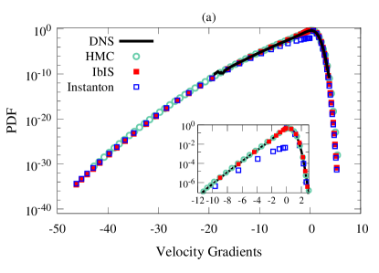
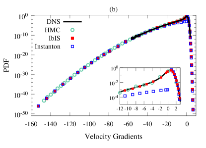
Figure 3: Velocity gradients PDF. Reweighted IbIS (red filled squares) and HMC (green open circles) versus the DNS (black line) and the instanton (open blue squares) (a) $N_{x}=64$, $N_{t}=576$, $\nu=0.5$, scanning for $a\in(-46,5)$. (b) $N_{x}=256$, $N_{t}=1152$, $\nu=0.2$, scanning for $a\in(-160,10)$.

We performed two sets of simulations for two different Reynolds numbers determined by the prescribed viscosities $\nu=0.5$ and $\nu=0.2$. A set consists of i) direct numerical simulations (DNS) of the Burgers equation, ii) a hybrid Monte Carlo Margazoglou et al. (2018) (HMC) sampling of the path integral and iii) our instanton based importance sampling (IbIS).

The hybrid Monte Carlo approach utilizes the action $S_{\mathcal{L}}$ (6) that depends on the flow configuration and constructs the measure as a weighted sum of all possible flow-realizations. Then $S_{\mathcal{L}}$ together with an additional gradient maximization constraint

$$S^{\prime}=S_{\mathcal{L}}+c_{1}u_{x}(0,0)$$ (29)

is sampled via the HMC algorithm Duane et al. (1987), where the prefactor $c_{1}$ defines the strength of the constraint. The choice of the additional functional can, in principle, be arbitrary, here it is specifically designed to systematically generate a large (positive, if $c_{1}<0$ or negative, if $c_{1}>0$) velocity gradient at a specified space-time point, here at $(x,t)=(0,0)$. Hence, the system favors the sampling of extreme and rare events in a similar spirit as an a posteriori filtering of strong gradient events generated by a standard DNSGrafke, Grauer, and Schäfer (2013).

To test its validity and capabilities, the IbIS method is put in comparison to the HMC and the DNS by measuring the PDF of the velocity gradients. Both the IbIS and the HMC consider the reweighted statistics of the velocity gradient measured only at $(x,t)=(0,0)$ (as explained in Sec. IV.1 and in Margazoglou et al. (2018)), while for the DNS we consider any site that belongs to the stationary regime. In Figs. 3(a,b) we compare the cases of $\nu=0.5$ and $\nu=0.2$, respectively. The inlet plot is an enlargement of the central region of the PDF, to strain that both reweighted PDFs of IbIS and HMC, successfully reproduce it. On the other hand, as expected, the instanton prediction for small negative velocity gradients is wrong and underestimates the real PDF, as in this region the instanton approach is invalid, while in the case of the right tails the instanton prediction is exactGurarie and Migdal (1996). Most importantly, the far left tail of the PDFs is reproduced identically both from the IbIS and the HMC simulations. In addition, the PDFs approach the instanton prediction for increasing $|u_{x}|$ as it is stated by large deviation theory. This also constitutes a proof of concept of the IbIS method, as both implementations are completely different and independent.

In Fig. 4 we plot the relative error of the bins in Fig. 3(a). We notice that in the case of the DNS, the errors quickly deviate for large velocity gradients due to the sparsity of the measurements. This result is expected and underlines the need for rare-event algorithms in turbulence. Contrary to the direct numerical simulations, both the IbIS and the HMC provide sufficient statistics, resulting to constant and controllable small relative errors over a substantially extended range of values of the PDF of velocity gradient fluctuations ${\cal P}(u_{x})$. In this respect, both the HMC and IbIS strategy are of comparable quality to capture rare events in turbulence.

The difference between the HMC and the IbIS methods is captured in Table 1. This table does not only show all parameters used in our simulations, but most importantly the run-time used for the different simulations. First, we note the run-time for the DNS is about the size (or even smaller) than the run-time used in the HMC simulations. However, we stress that the DNS is only capable to capture a tiny fraction of the PDF. The remarkable effectiveness of the IbIS compared to the HMC method can be deduced from the ratio of their computing times. Here for the parameters used in our test cases, the IbIS method turns out to be two orders of magnitudes faster than the HMC approach, a ratio that is even expected to increase for higher Reynolds numbers.

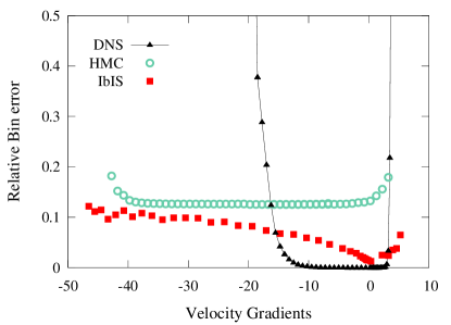
Figure 4: Relative bin errors of the velocity gradient PDFs of Fig. 3(a). The errors of the DNS quickly deviate, while the errors of the IbIS and the HMC stay small and under control.

V Conclusions and Outlook

In this paper we have presented a new method based on instanton importance sampling to calculate the probability distribution function of velocity gradients in Burgers equation for both typical and extremely intense events. By sampling fluctuations of the SPDE obtained on the background of one given instanton with a fixed (negative) intense velocity gradient in a certain $(x,t)$ position, we explore the fluctuations around that specific flow configuration. At varying the reference gradient, and with a suitable reweighting protocol, we are able to reconstruct the whole PDF. The method is fully general and can –in principle– be applied to any SPDE. To be successful, a necessary condition is that a large deviation principle is applicable that guarantees the availability of unique instanton solutions. The IbIS method will work most efficiently when the PDF obtained solely from the instanton prediction is not to far from the true PDF. We also compared this new method with a Hybrid Monte Carlo approach Margazoglou et al. (2018) which does not rely on these assumptions and thus is applicable to a larger variety of physical problems. Concerning the Burgers case, IbIS is orders of magnitudes faster then the HMC. Both methods are much better than standard pseudo-spectral algorithms which are unable to focus on extreme-rare events. With the IbIS method it might be possible to calculate the scaling of the algebraic power law prefactors, which characterizes the inviscid limit of Burgers equations W. et al. (1997); E and Vanden Eijnden (2000) without using Lagrangian particle and shock tracking methodsBec (2001).