Equivalence of pushdown automata via first-order grammars

Abstract

A decidability proof for bisimulation equivalence of first-order grammars is given. It is an alternative proof for a result by Sénizergues (1998, 2005) that subsumes his affirmative solution of the famous decidability question for deterministic pushdown automata.

The presented proof is conceptually simpler, and a particular novelty is that it is not given as two semidecision procedures but it provides an explicit algorithm that might be amenable to a complexity analysis.

1 Introduction

Decision problems for semantic equivalences have been a frequent topic in computer science. For pushdown automata (PDA) language equivalence was quickly shown undecidable, while the decidability in the case of deterministic PDA (DPDA) is a famous result by Sénizergues [1]. A finer equivalence, called bisimulation equivalence or bisimilarity, has emerged as another fundamental behavioural equivalence [2]; for deterministic systems it essentially coincides with language equivalence. By [3] we can exemplify the first decidability results for infinite-state systems (a subclass of PDA, in fact), and refer to [4] for a survey of results in a relevant area.

One of the most involved results in this area shows the decidability of bisimilarity of equational graphs with finite out-degree, which are equivalent to PDA with alternative-free $\varepsilon$-steps (if an $\varepsilon$-step is enabled, then it has no alternative); Sénizergues [5] has thus generalized his decidability result for DPDA.

We recall that the complexity of the DPDA problem remains far from clear, the problem is known to be PTIME-hard and to be in TOWER (i.e., in the first complexity class beyond elementary in the terminology of [6]); the upper bound was shown by Stirling [7] (and formulated more explicitly in [8]). For PDA the bisimulation equivalence problem is known to be nonelementary [9] (in fact, TOWER-hard), even for real-time PDA, i.e. PDA with no $\varepsilon$-steps. For the above mentioned PDA with alternative-free $\varepsilon$-steps the problem is even not primitive recursive; its Ackermann-hardness was shown in [8].

The decidability proofs, both for DPDA and PDA, are involved and hard to understand. This paper aims to contribute to a clarification of the more general decidability proof, showing an algorithm deciding bisimilarity of PDA with alternative-free $\varepsilon$-steps.

The proof is shown in the framework of labelled transition systems generated by first-order grammars (FO-grammars), which seems to be a particularly convenient formalism; it is called term context-free grammars in [10]. Here the states (or configurations) are first-order terms over a specified finite set of function symbols (or “nonterminals”); the transitions are induced by a first-order grammar, which is a finite set of labelled rules for rewriting the roots of terms. This framework is equivalent to the framework of [5]; cf., e.g., [11, 10] and the references therein, or also [12] for a concrete transformation of PDA to FO-grammars. The proof here is in principle based on the high-level ideas from the proof in [5] but with various simplifications and new modifications. The presented proof has resulted by a thorough reworking of the conference paper [13], aiming to get an algorithm that might be amenable to a complexity analysis.

Proof overview. We give a flavour of the process that is formally realized in the paper. It is standard to characterize bisimulation equivalence (also called bisimilarity) in terms of a turn-based game between Attacker and Defender, say. If two PDA-configurations, modelled by first-order terms $E,F$ in our framework, are non-bisimilar, then Attacker can force his win within $k$ rounds of the game, for some number $k\in\mathbb{N}$; in this case $k{-}1$ for the least such $k$ can be viewed as the equivalence-level $\textsc{el}(E,F)$ of terms $E,F$: we write $E\sim_{k-1}F$ and $E\not\sim_{k}F$. If $E,F$ are bisimilar, i.e. $E\sim F$, then Defender has a winning strategy and we put $\textsc{el}(E,F)=\omega$. A natural idea is to search for a computable function $f$ attaching a number $f(\mathcal{G},E,F)\in\mathbb{N}$ to terms $E,F$ and a grammar $\mathcal{G}$ so that it is guaranteed that $\textsc{el}(E,F)\leq f(\mathcal{G},E,F)$ or $\textsc{el}(E,F)=\omega$; this immediately yields an algorithm that computes $\textsc{el}(E,F)$ (concluding that $\textsc{el}(E,F)=\omega$ when finding that $\textsc{el}(E,F)>f(\mathcal{G},E,F)$).

We will show such a computable function $f$ by analysing optimal plays from $E_{0}\not\sim F_{0}$; such an optimal play gives rise to a sequence $(E_{0},F_{0})$, $(E_{1},F_{1})$, $\dots$, $(E_{k},F_{k})$ of pairs of terms where $\textsc{el}(E_{i},F_{i})=\textsc{el}(E_{i-1},F_{i-1})-1$ for $i=1,2,\dots,k$, and $\textsc{el}(E_{k},F_{k})=0$ (hence $\textsc{el}(E_{0},F_{0})=k$). This sequence is then suitably modified to yield a certain sequence

$$(E^{\prime}_{0},F^{\prime}_{0}),(E^{\prime}_{1},F^{\prime}_{1}),\dots,(E^{\prime}_{k},F^{\prime}_{k})$$ (1)

such that $(E^{\prime}_{0},F^{\prime}_{0})=(E_{0},F_{0})$ and $\textsc{el}(E^{\prime}_{i},F^{\prime}_{i})=\textsc{el}(E_{i},F_{i})$ for all $i=1,2,\dots,k$; here we use simple congruence properties (if $E^{\prime}$ arises from $E$ by replacing a subterm $H$ with $H^{\prime}$ such that $H\sim_{k}H^{\prime}$, then $E\sim_{k}E^{\prime}$). Doing this modification carefully, adhering to a sort of “balancing policy” (inspired by one crucial ingredient in [1, 5], used also in [14]) we derive that if $k$ is “large”, then the sequence (1) contains a “long” subsequence

$$(\overline{E}_{1}\sigma,\overline{F}_{1}\sigma),(\overline{E}_{2}\sigma,\overline{F}_{2}\sigma),\dots,(\overline{E}_{z}\sigma,\overline{F}_{z}\sigma),$$ (2)

called an $(n,s,g)$-sequence, where the variables in all “tops” $\overline{E}_{j}$, $\overline{F}_{j}$ are from the set $\{x_{1},\dots,x_{n}\}$, $\sigma$ is the common “tail” substitution (maybe with “large” terms $x_{i}\sigma$), and the size-growth of the tops is bounded: $\textsc{Size}(\overline{E}_{j},\overline{F}_{j})\leq s+g\cdot(j{-}1)$ for $j=1,2,\dots,z$. The numbers $n,s,g$ are elementary in the size of the grammar $\mathcal{G}$. Then another fact is used (whose analogues in different frameworks could be traced back to [1, 5] and other related works): if $\textsc{el}(\overline{E}_{1},\overline{F}_{1})=e<\ell=\textsc{el}(\overline{E}_{1}\sigma,\overline{F}_{1}\sigma)$, then there is $i\in\{1,2,\dots,n\}$ and a term $H\neq x_{i}$ reachable from $\overline{E}_{1}$ or $\overline{F}_{1}$ within $e$ moves (i.e. root-rewriting steps) such that $x_{i}\sigma\sim_{\ell-e}H\sigma$. This entails that for $j=e{+}2,e{+}3,\dots,z$ the tops $(\overline{E}_{j},\overline{F}_{j})$ in (2) can be replaced with $(\overline{E}_{j}[x_{i}/H^{\prime}],\overline{F}_{j}[x_{i}/H^{\prime}])$, where $H^{\prime}$ is the regular term $H[x_{i}/H][x_{i}/H][x_{i}/H]\cdots$, without changing the equivalence-level; hence $\textsc{el}(\overline{E}_{j}\sigma,\overline{F}_{j}\sigma)=\textsc{el}(\overline{E}_{j}[x_{i}/H^{\prime}]\sigma,\overline{F}_{j}[x_{i}/H^{\prime}]\sigma)$. Though $H^{\prime}$ might be an infinite regular term, its natural graph presentation is not larger than the presentation of $H$. Moreover, $x_{i}$ does not occur in $H^{\prime}$, and thus the term $x_{i}\sigma$ ceases to play any role in the pairs $(\overline{E}_{j}[x_{i}/H^{\prime}]\sigma,\overline{F}_{j}[x_{i}/H^{\prime}]\sigma)$ ($j=e{+}2,e{+}3,\dots,z$).

By continuing this reasoning inductively (“removing” one $x_{i}\sigma$ in each of at most $n$ phases), we note that the length of $(n,s,g)$-sequences (2) is bounded by a (maybe large) constant determined by the grammar $\mathcal{G}$. By a careful analysis we then show that such a constant is, in fact, computable when a grammar is given.

Further remarks on related research. Further work is needed to fully understand the bisimulation problems on PDA and their subclasses, also regarding their computational complexity. E.g., even the case of BPA processes, generated by real-time PDA with a single control-state, is not quite clear. Here the bisimilarity problem is EXPTIME-hard [15] and in 2-EXPTIME [16] (proven explicitly in [17]); for the subclass of normed BPA the problem is polynomial [18] (see [19] for the best published upper bound). Another issue is the precise decidability border. This was also studied in [20]; allowing that $\varepsilon$-steps can have alternatives (though they are restricted to be stack-popping) leads to undecidability of bisimilarity. This aspect has been also refined, for branching bisimilarity [21]. For second-order PDA the undecidability is established without $\varepsilon$-steps [22]. We can refer to the survey papers [23, 24] for the work on higher-order PDA, and in particular mention that the decidability of equivalence of deterministic higher-order PDA remains open; some progress in this direction was made by Stirling in [25].

Finally we remark that recently (while this paper was under review) the author cooperated with Sylvain Schmitz on developing a concrete version of the algorithm suggested here, and its complexity analysis has revealed an Ackermannian upper bound; with the lower bound from [8] this yields the Ackermann-completeness of the studied equivalence problem [26].

Organization of the paper. After the preliminaries in Section 2 we state the main theorem in Section 3. The theorem is proven in Section 7, using the notions and results discussed in Sections 4, 5, and 6; each of these sections starts with an informal summary.

2 Basic Notions and Facts

In this section we define basic notions and observe their simple properties. Some standard definitions are restricted when we do not need full generality.

By $\mathbb{N}$ and $\mathbb{N}_{+}$ we denote the sets of nonnegative integers and of positive integers, respectively. By $[i,j]$, for $i,j\in\mathbb{N}$, we denote the set $\{i,i{+}1,\dots,j\}$. For a set $\mathcal{A}$, by $\mathcal{A}^{*}$ we denote the set of finite sequences of elements of $\mathcal{A}$, which are also called words (over $\mathcal{A}$). By $|w|$ we denote the length of $w\in\mathcal{A}^{*}$, and by $\varepsilon$ the empty sequence; hence $|\varepsilon|=0$. We put $\mathcal{A}^{+}=\mathcal{A}^{*}\smallsetminus\{\varepsilon\}$.

Labelled transition systems.

A labelled transition system, an LTS for short, is a tuple $\mathcal{L}=(\mathcal{S},\Sigma,(\xrightarrow{a})_{a\in{\Sigma}})$ where $\mathcal{S}$ is a finite or countable set of states, $\Sigma$ is a finite or countable set of actions and $\xrightarrow{a}\mathop{\subseteq}\mathcal{S}\times\mathcal{S}$ is a set of $a$-transitions (for each $a\in\Sigma$). We say that $\mathcal{L}$ is a deterministic LTS if for each pair $s\in\mathcal{S}$, $a\in\Sigma$ there is at most one $s^{\prime}$ such that $s\xrightarrow{a}s^{\prime}$ (which stands for $(s,s^{\prime})\mathop{\in}\xrightarrow{a}$). By $s\xrightarrow{w}s^{\prime}$, where $w=a_{1}a_{2}\dots a_{n}\in\Sigma^{*}$, we denote that there is a path $s=s_{0}\xrightarrow{a_{1}}s_{1}\xrightarrow{a_{2}}s_{2}\cdots\xrightarrow{a_{n}}s_{n}=s^{\prime}$; the length of such a path is $n$, which is zero for the (trivial) path $s\xrightarrow{\varepsilon}s$. If $s\xrightarrow{w}s^{\prime}$, then $s^{\prime}$ is reachable from $s$. By $s\xrightarrow{w}$ we denote that $w$ is enabled in $s$, or $w$ is performable from $s$, i.e., $s\xrightarrow{w}s^{\prime}$ for some $s^{\prime}$. If $\mathcal{L}$ is deterministic, then the expressions $s\xrightarrow{w}s^{\prime}$ and $s\xrightarrow{w}$ also denote a unique path.

Bisimilarity, eq-levels.

Given $\mathcal{L}=(\mathcal{S},\Sigma,(\xrightarrow{a})_{a\in\Sigma})$, a set $\mathcal{D}\subseteq\mathcal{S}\times\mathcal{S}$ covers $(s,t)\in\mathcal{S}\times\mathcal{S}$ if for any $s\xrightarrow{a}s^{\prime}$ there is $t\xrightarrow{a}t^{\prime}$ such that $(s^{\prime},t^{\prime})\in\mathcal{D}$, and for any $t\xrightarrow{a}t^{\prime}$ there is $s\xrightarrow{a}s^{\prime}$ such that $(s^{\prime},t^{\prime})\in\mathcal{D}$. For $\mathcal{D},\mathcal{D}^{\prime}\subseteq\mathcal{S}\times\mathcal{S}$ we say that $\mathcal{D}^{\prime}$ covers $\mathcal{D}$ if $\mathcal{D}^{\prime}$ covers each $(s,t)\in\mathcal{D}$. A set $\mathcal{D}\subseteq\mathcal{S}\times\mathcal{S}$ is a bisimulation if $\mathcal{D}$ covers $\mathcal{D}$. States $s,t\in\mathcal{S}$ are bisimilar, written $s\sim t$, if there is a bisimulation $\mathcal{D}$ containing $(s,t)$. A standard fact is that $\sim\,\subseteq\mathcal{S}\times\mathcal{S}$ is an equivalence relation, and it is the largest bisimulation, namely the union of all bisimulations.

We also put $\sim_{0}=\mathcal{S}\times\mathcal{S}$, and define $\sim_{k+1}\subseteq\mathcal{S}\times\mathcal{S}$ (for $k\in\mathbb{N}$) as the set of pairs covered by $\sim_{k}$. It is obvious that $\sim_{k}$ are equivalence relations, and that $\sim_{0}\,\supseteq\,\sim_{1}\,\supseteq\,\sim_{2}\,\supseteq\,\cdots\cdots\supseteq\sim$. For the (first limit) ordinal $\omega$ we put $s\sim_{\omega}t$ if $s\sim_{k}t$ for all $k\in\mathbb{N}$; hence $\sim_{\omega}=\bigcap_{k\in\mathbb{N}}\sim_{k}$. We will only consider image-finite LTSs, where the set $\{s^{\prime}\mid s\xrightarrow{a}s^{\prime}\}$ is finite for each pair $s\in\mathcal{S}$, $a\in\Sigma$. In this case $\bigcap_{k\in\mathbb{N}}\sim_{k}$ is a bisimulation (for each $(s,t)\in\bigcap_{k\in\mathbb{N}}\sim_{k}$ and $s\xrightarrow{a}s^{\prime}$, in the finite set $\{t^{\prime}\mid t\xrightarrow{a}t^{\prime}\}$ there must be one $t^{\prime}$ such that $s^{\prime}\sim_{k}t^{\prime}$ for infinitely many $k$, which entails $(s^{\prime},t^{\prime})\in\bigcap_{k\in\mathbb{N}}\sim_{k}$), and thus $\sim\,=\bigcap_{k\in\mathbb{N}}\sim_{k}\,=\,\sim_{\omega}$.

To each pair of states $s,t$ we attach their equivalence level (eq-level):

$\textsc{el}(s,t)=\max\,\{k\in\mathbb{N}\cup\{\omega\}\mid s\sim_{k}t\}$.

Hence $\textsc{el}(s,t)=0$ iff $\{a\in\Sigma\mid s\xrightarrow{a}\}\neq\{a\in\Sigma\mid t\xrightarrow{a}\}$ (i.e., $s$ and $t$ enable different sets of actions). The next proposition captures a few additional simple facts; we should add that we handle $\omega$ as an infinite amount, stipulating $\omega>n$ and $\omega+n=\omega-n=\omega$ for all $n\in\mathbb{N}$.

Proposition 1.

1. If $\textsc{el}(t,t^{\prime})>\textsc{el}(s,t)$, then $\textsc{el}(s,t)=\textsc{el}(s,t^{\prime})$.

2. If $\omega>\textsc{el}(s,t)>0$, then there is either a transition $s\xrightarrow{a}s^{\prime}$ such that for all transitions $t\xrightarrow{a}t^{\prime}$ we have $\textsc{el}(s^{\prime},t^{\prime})\leq\textsc{el}(s,t)-1$, or a transition $t\xrightarrow{a}t^{\prime}$ such that for all transitions $s\xrightarrow{a}s^{\prime}$ we have $\textsc{el}(s^{\prime},t^{\prime})\leq\textsc{el}(s,t)-1$.

3. If $|w|\leq\textsc{el}(s,t)$ and $s\xrightarrow{w}s^{\prime}$, then $t\xrightarrow{w}t^{\prime}$ for $t^{\prime}$ such that $\textsc{el}(s^{\prime},t^{\prime})\geq\textsc{el}(s,t)-|w|$.

Proof.

1. If $s\sim_{k}t$, $s\not\sim_{k+1}t$, and $t\sim_{k+1}t^{\prime}$, then $s\sim_{k}t^{\prime}$ and $s\not\sim_{k+1}t^{\prime}$.

The points 2 and 3 trivially follow from the definition of $\sim_{k}$ (for $k\in\mathbb{N}\cup\{\omega\}$). ∎

First-order terms, regular terms, finite graph presentations.

We will consider LTSs in which the states are first-order regular terms.

The terms are built from variables taken from a fixed countable set

$$\textsc{Var}=\{x_{1},x_{2},x_{3},\dots\}$$

and from function symbols, also called (ranked) nonterminals, from some specified finite set $\mathcal{N}$; each $A\in\mathcal{N}$ has $arity(A)\in\mathbb{N}$. We reserve symbols $A,B,C,D$ to range over nonterminals, and $E,F,G,H,T,U,V,W$ to range over terms. An example of a finite term is $E_{1}=A(D(x_{5},C(x_{2},B)),x_{5},B)$, where the arities of nonterminals $A,B,C,D$ are $3,0,2,2$, respectively. Its syntactic tree is depicted on the left of Fig.1.

Figure 1: Finite terms $E_{1}$, $E_{2}$, and a graph presenting a regular infinite term $E_{3}$

We identify terms with their syntactic trees. Thus a term over $\mathcal{N}$ is (viewed as) a rooted, ordered, finite or infinite tree where each node has a label from $\mathcal{N}\cup\textsc{Var}$; if the label of a node is $x\in\textsc{Var}$, then the node has no successors, and if the label is $A\in\mathcal{N}$, then it has $m$ (immediate) successor-nodes where $m=arity(A)$. A subtree of a term $E$ is also called a subterm of $E$. We make no difference between isomorphic (sub)trees, and thus a subterm can have more (maybe infinitely many) occurrences in $E$. Each subterm-occurrence has its (nesting) depth in $E$, which is its (naturally defined) distance from the root of $E$. E.g., $C(x_{2},B)$ is a depth-2 subterm of $E_{1}$; $x_{5}$ is a subterm with a depth-1 and a depth-2 occurrences.

We also use the standard notation for terms: we write $E=x_{i}$ or $E=A(G_{1},\dots,G_{m})$ with the obvious meaning; in the latter case $\textsc{root}(E)=A\in\mathcal{N}$, $m=arity(A)$, and $G_{1},\dots,G_{m}$ are the ordered depth-$1$ occurrences of subterms of $E$, which are also called the root-successors in $E$.

A term is finite if the respective tree is finite. A (possibly infinite) term is regular if it has only finitely many subterms (though the subterms may be infinite and may have infinitely many occurrences). We note that any regular term has at least one graph presentation, i.e. a finite directed graph with a designated root, where each node has a label from $\mathcal{N}\cup\textsc{Var}$; if the label of a node is $x\in\textsc{Var}$, then the node has no outgoing arcs, if the label is $A\in\mathcal{N}$, then it has $m$ ordered outgoing arcs where $m=arity(A)$. We can see an example of such a graph presenting a term $E_{3}$ on the right in Fig. 1. The standard tree-unfolding of the graph is the respective term, which is infinite if there are cycles in the graph. There is a bijection between the nodes in the least graph presentation of $E$ and (the roots of) the subterms of $E$.

Sizes, heights, and variables of terms.

By $\textsc{Terms}_{\mathcal{N}}$ we denote the set of all regular terms over $\mathcal{N}$ (and Var); we do not consider non-regular terms. By a “term” we mean a general regular term unless the context makes clear that the term is finite.

By $\textsc{Size}(E)$ we mean the number of nodes in the least graph presentation of $E$. E.g., in Fig.1 $\textsc{Size}(E_{1})=6$ ($E_{1}$ has six subterms) and $\textsc{Size}(E_{3})=5$. By $\textsc{Size}(\{E_{1},E_{2},\dots,E_{n}\})$ we mean the number of nodes in the least graph presentation in which a distinguished node $\textsc{r}_{i}$ corresponds to the (root of the) term $E_{i}$, for each $i\in[1,n]$. (Since $E_{1},E_{2},\dots,E_{n}$ can share some subterms, $\textsc{Size}(\{E_{1},E_{2},\dots,E_{n}\})$ can be smaller than $\sum_{i\in[1,n]}\textsc{Size}(E_{i})$.) We usually write $\textsc{Size}(E,F)$ instead of $\textsc{Size}(\{E,F\})$. E.g., $\textsc{Size}(E_{1},E_{2})=9$ in Fig. 1.

For a finite term $E$ we define $0pt(E)$ as the maximal depth of a subterm; e.g., $0pt(E_{1})=3$ in Fig.1.

We put $\textsc{var}(E)=\{x\in\textsc{Var}\mid x$ occurs in $E\}$ and $\textsc{var}(E,F)=\{x\in\textsc{Var}\mid x$ occurs in $E$ or $F\}$. E.g., $\textsc{var}(E_{1},E_{2})=\{x_{2},x_{5}\}$ in Fig.1.

Substitutions, associative composition, iterated substitutions.

A substitution $\sigma$ is a mapping $\sigma:\textsc{Var}\rightarrow\textsc{Terms}_{\mathcal{N}}$ whose support

$\textsc{supp}(\sigma)=\{x\in\textsc{Var}\mid\sigma(x)\neq x\}$

is finite; we reserve the symbol $\sigma$ for substitutions. By applying a substitution $\sigma$ to a term $E$ we get the term $E\sigma$ that arises from $E$ by replacing each occurrence of $x\in\textsc{Var}$ with $\sigma(x)$; given graph presentations, in the graph of $E$ we just redirect each arc leading to a node labelled with $x$ towards the root of $\sigma(x)$ (which includes the special “root-designating arc” when $E=x$). Hence $E=x$ implies $E\sigma=x\sigma=\sigma(x)$. The natural composition of substitutions, where $\sigma=\sigma_{1}\sigma_{2}$ is defined by $x\sigma=(x\sigma_{1})\sigma_{2}$, can be easily verified to be associative. We thus write $E\sigma_{1}\sigma_{2}$ instead of $(E\sigma_{1})\sigma_{2}$ or $E(\sigma_{1}\sigma_{2})$. For $i\in\mathbb{N}$ we define $\sigma^{i}$ inductively: $\sigma^{0}$ is the empty-support substitution, and $\sigma^{i+1}=\sigma\sigma^{i}$.

By $[x_{i_{1}}/H_{1},x_{i_{2}}/H_{2},\dots,x_{i_{k}}/H_{k}]$, where $i_{j}\neq i_{j^{\prime}}$ for $j\neq j^{\prime}$, we denote the substitution $\sigma$ such that $x_{i_{j}}\sigma=H_{j}$ for all $j\in[1,k]$ and $x\sigma=x$ for all $x\in\textsc{Var}\smallsetminus\{x_{i_{1}},x_{i_{2}},\dots,x_{i_{k}}\}$. We will use $\sigma^{\omega}=\sigma\sigma\sigma\cdots$ just for the special case $\sigma=[x_{i}/H]$, where $\sigma^{\omega}$ is clearly well-defined; a graph presentation of the term $x_{i}\sigma^{\omega}$ arises from a graph presentation of $H$ by redirecting each arc leading to $x_{i}$ (if any exists) towards the root; we have $x_{i}\sigma^{\omega}=H$ if $x_{i}\not\in\textsc{var}(H)$, or if $H=x_{i}$. In Fig.1, for $\sigma=[x_{2}/E_{1}]$ we have $E_{2}=E_{1}\sigma$ and $E_{3}=E_{1}\sigma^{\omega}$.

By $\sigma_{[-x_{i}]}$ we denote the substitution arising from $\sigma$ by removing $x_{i}$ from its support (if it is there): hence $x_{i}\sigma_{[-x_{i}]}=x_{i}$ and $x\sigma_{[-x_{i}]}=x\sigma$ for all $x\in\textsc{Var}\smallsetminus\{x_{i}\}$.

We note a trivial fact (for later use):

Proposition 2.

If $H\neq x_{i}$, then for the term $H^{\prime}=H[x_{i}/H][x_{i}/H][x_{i}/H]\cdots$ we have $x_{i}\not\in\textsc{var}(H^{\prime})$, and thus $H^{\prime}\sigma=H^{\prime}\sigma_{[-x_{i}]}$ for any $\sigma$. We also have $\textsc{Size}(H^{\prime})\leq\textsc{Size}(H)$.

First-order grammars.

A first-order grammar, or just a grammar for short, is a tuple $\mathcal{G}=(\mathcal{N},\Sigma,\mathcal{R})$ where $\mathcal{N}$ is a finite nonempty set of ranked nonterminals, viewed as function symbols with arities, $\Sigma$ is a finite nonempty set of actions (or “letters”), and $\mathcal{R}$ is a finite nonempty set of rules of the form

$$A(x_{1},x_{2},\dots,x_{m})\xrightarrow{a}E$$ (3)

where $A\in\mathcal{N}$, $arity(A)=m$, $a\in\Sigma$, and $E$ is a finite term over $\mathcal{N}$ in which each occurring variable is from the set $\{x_{1},x_{2},\dots,x_{m}\}$; we can have $E=x_{i}$ for some $i\in[1,m]$.

LTSs generated by rules, and by actions, of grammars.

Given $\mathcal{G}=(\mathcal{N},\Sigma,\mathcal{R})$, by $\mathcal{L}^{\textsc{r}}_{\mathcal{G}}$ we denote the (rule-based) LTS $\mathcal{L}^{\textsc{r}}_{\mathcal{G}}=(\textsc{Terms}_{\mathcal{N}},\mathcal{R},(\xrightarrow{r})_{r\in\mathcal{R}})$ where each rule $r$ of the form $A(x_{1},x_{2},\dots,x_{m})\xrightarrow{a}E$ induces transitions $A(x_{1},\dots,x_{m})\sigma\xrightarrow{r}E\sigma$ for all substitutions $\sigma$. The transition induced by $\sigma$ with $\textsc{supp}(\sigma)=\emptyset$ is $A(x_{1},\dots,x_{m})\xrightarrow{r}E$.

Using terms from Fig.1 as examples, if a rule $r_{1}$ is $A(x_{1},x_{2},x_{3})\xrightarrow{b}x_{2}$, then we have $E_{3}\xrightarrow{r_{1}}x_{5}$ (since $E_{3}$ can be written as $A(x_{1},x_{2},x_{3})\sigma$ where $x_{2}\sigma=x_{5}$); the action $b$ only plays a role in the LTS $\mathcal{L}^{\textsc{a}}_{\mathcal{G}}$ defined below (where we have $E_{3}\xrightarrow{b}x_{5}$). For a rule $r_{2}:A(x_{1},x_{2},x_{3})\xrightarrow{a}C(x_{2},D(x_{2},x_{1}))$ we deduce $E_{1}\xrightarrow{r_{2}}C(x_{5},D(x_{5},D(x_{5},C(x_{2},B))))$; we note that the third root-successor in $E_{1}$ thus “disappears” since $x_{3}\not\in\textsc{var}(C(x_{2},D(x_{2},x_{1})))$.

By definition, the LTS $\mathcal{L}^{\textsc{r}}_{\mathcal{G}}$ is deterministic (for each $F$ and $r$ there is at most one $H$ such that $F\xrightarrow{r}H$). We note that variables are dead (have no outgoing transitions). We also note that $F\xrightarrow{w}H$ implies $\textsc{var}(H)\subseteq\textsc{var}(F)$ (each variable occurring in $H$ also occurs in $F$) but not $\textsc{var}(F)\subseteq\textsc{var}(H)$ in general.

Remark. Since the rhs (right-hand sides) $E$ in the rules (3) are finite, all terms reachable from a finite term are finite. The “finite-rhs version” with general regular terms in LTSs has been chosen for technical convenience. This is not crucial, since the equivalence problem for the “regular-rhs version” can be easily reduced to the problem for our finite-rhs version.

The deterministic rule-based LTS $\mathcal{L}^{\textsc{r}}_{\mathcal{G}}$ is helpful technically, but we are primarily interested in the (image-finite nondeterministic) action-based LTS $\mathcal{L}^{\textsc{a}}_{\mathcal{G}}=(\textsc{Terms}_{\mathcal{N}},\Sigma,(\xrightarrow{a})_{a\in\Sigma})$ where each rule $A(x_{1},\dots,x_{m})\xrightarrow{a}E$ induces the transitions $A(x_{1},\dots,x_{m})\sigma\xrightarrow{a}E\sigma$ for all substitutions $\sigma$. (Hence the rules $r_{1}$ and $r_{2}$ in the above examples induce $E_{3}\xrightarrow{b}x_{5}$ and $E_{1}\xrightarrow{a}C(x_{5},D(x_{5},D(x_{5},C(x_{2},B))))$.)

Fig.2 sketches a path in some LTS $\mathcal{L}^{\textsc{r}}_{\mathcal{G}}$ where we have, e.g., $r_{1}:A(x_{1},x_{2},x_{3})\xrightarrow{a_{1}}C(D(x_{2},x_{3}),x_{3})$ and $r_{2}:C(x_{1},x_{2})\xrightarrow{a_{2}}x_{2}$ for some actions $a_{1},a_{2}$ (which would replace $r_{1},r_{2}$ in the LTS $\mathcal{L}^{\textsc{a}}_{\mathcal{G}}$). In the rectangle just a part of a regular-term presentation is sketched. Hence the initial root-node $A$ might be accessible from later roots due to its possible undepicted ingoing arcs. On the other hand, the root-node $D$ after the steps $r_{1}r_{2}r_{3}$ is not accessible (and can be omitted) in the presentation of the final term.

Figure 2: Path $A(T_{1},T_{2},B(T_{3},T_{4}))\xrightarrow{r_{1}}C(D(T_{2},B(T_{3},T_{4})),B(T_{3},T_{4}))\xrightarrow{r_{2}}B(T_{3},T_{4})\xrightarrow{r_{3}r_{4}}$ in $\mathcal{L}^{\textsc{r}}_{\mathcal{G}}$

Eq-levels of pairs of terms.

Given a grammar $\mathcal{G}=(\mathcal{N},\Sigma,\mathcal{R})$, by $\textsc{el}(E,F)$ we refer to the equivalence level of (regular) terms $E,F$ in $\mathcal{L}^{\textsc{a}}_{\mathcal{G}}$, with the following adjustment: though variables $x_{i}$ are handled as dead also in $\mathcal{L}^{\textsc{a}}_{\mathcal{G}}$, we stipulate $\textsc{el}(x_{i},H)=0$ if $H\neq x_{i}$ (while $\textsc{el}(x_{i},x_{i})=\omega$); this would be achieved automatically if we enriched $\mathcal{L}^{\textsc{a}}_{\mathcal{G}}$ with transitions $x\xrightarrow{a_{x}}x$ where $a_{x}$ is a special action added to each variable $x\in\textsc{Var}$. This adjustment gives us the point $1$ in the next proposition on compositionality.

We put $\sigma\sim_{k}\sigma^{\prime}$ if $x\sigma\sim_{k}x\sigma^{\prime}$ for all $x\in\textsc{Var}$, and define

$\textsc{el}(\sigma,\sigma^{\prime})=\max\big{\{}k\in\mathbb{N}\cup\{\omega\}\mid\sigma\sim_{k}\sigma^{\prime}\big{\}}$.

Proposition 3.

For all $\sigma,\sigma^{\prime},\sigma^{\prime\prime},E,F$, and $k\in\mathbb{N}\cup\{\omega\}$ the following conditions hold:

1. If $\sigma^{\prime}\sim_{k}\sigma^{\prime\prime}$, then $\sigma^{\prime}\sigma\sim_{k}\sigma^{\prime\prime}\sigma$. Hence $\textsc{el}(\sigma^{\prime},\sigma^{\prime\prime})\leq\textsc{el}(\sigma^{\prime}\sigma,\sigma^{\prime\prime}\sigma)$.

   In particular, $\textsc{el}(E,F)\leq\textsc{el}(E\sigma,F\sigma)$.

2. If $\sigma^{\prime}\sim_{k}\sigma^{\prime\prime}$, then $\sigma\sigma^{\prime}\sim_{k}\sigma\sigma^{\prime\prime}$. Hence $\textsc{el}(\sigma^{\prime},\sigma^{\prime\prime})\leq\textsc{el}(\sigma\sigma^{\prime},\sigma\sigma^{\prime\prime})$.

   In particular, $\textsc{el}(\sigma^{\prime},\sigma^{\prime\prime})\leq\textsc{el}(E\sigma^{\prime},E\sigma^{\prime\prime})$.

Proof.

It suffices to prove the claims for $k\in\mathbb{N}$, since $\sim_{\omega}=\bigcap_{k\in\mathbb{N}}\sim_{k}$. We use an induction on $k$, noting that for $k=0$ the claims are trivial.

Assuming $k>0$ and $E\sim_{k}F$, we show that $E\sigma\sim_{k}F\sigma$: We cannot have $\{E,F\}=\{x_{i},H\}$ for some $H\neq x_{i}$ (since then $\textsc{el}(E,F)=0$ by our definition). Hence either $E=F=x$ for some $x\in\textsc{Var}$, in which case $E\sigma=F\sigma$, or $E\not\in\textsc{Var}$ and $F\not\in\textsc{Var}$. In the latter case every transition $E\sigma\xrightarrow{a}G$ ($F\sigma\xrightarrow{a}G$) is, in fact, $E\sigma\xrightarrow{a}E^{\prime}\sigma$ ($F\sigma\xrightarrow{a}F^{\prime}\sigma$) where $E\xrightarrow{a}E^{\prime}$ ($F\xrightarrow{a}F^{\prime}$), and there must be a corresponding transition $F\xrightarrow{a}F^{\prime}$ ($E\xrightarrow{a}E^{\prime}$) such that $E^{\prime}\sim_{k-1}F^{\prime}$ (by Proposition 1(3)); by the induction hypothesis $E^{\prime}\sigma\sim_{k-1}F^{\prime}\sigma$, which shows that $E\sigma\sim_{k}F\sigma$ (since $(E\sigma,F\sigma)$ is covered by $\sim_{k-1}$).

This gives us the point $1$. For the point $2$ we note that $\sigma^{\prime}\sim_{k}\sigma^{\prime\prime}$ implies $E\sigma^{\prime}\sim_{k}E\sigma^{\prime\prime}$, which is even more straightforward to verify. ∎

The next lemma shows a simple but important fact (whose analogues in different frameworks could be traced back to [1, 5] and other related works). Its claim is sketched in a part of Figure 3. (We recall that $E,F$ denote general regular terms when we do not say that they are finite.)

Lemma 4.

If $\textsc{el}(E,F)=k<\ell=\textsc{el}(E\sigma,F\sigma)$, then there are $x_{i}\in\textsc{supp}(\sigma)$, $H\neq x_{i}$, and $w\in\Sigma^{*}$, $|w|\leq k$, such that $E\xrightarrow{w}x_{i}$, $F\xrightarrow{w}H$ or $E\xrightarrow{w}H$, $F\xrightarrow{w}x_{i}$, and $x_{i}\sigma\sim_{\ell-k}H\sigma$.

Proof.

We assume $\textsc{el}(E,F)=k<\ell=\textsc{el}(E\sigma,F\sigma)$ and use an induction on $k$. If $k=0$, then necessarily $\{E,F\}=\{x_{i},H\}$ for some $x_{i}\neq H$ (since $E\not\in\textsc{Var}$, $F\not\in\textsc{Var}$ would imply $\textsc{el}(E\sigma,F\sigma)=0$ as well); the claim is thus trivial (if $x_{i}\not\in\textsc{supp}(\sigma)$, i.e. $x_{i}\sigma=x_{i}$, then $H=x_{j}$ and $x_{j}\sigma=x_{i}$, which entails that $x_{j}\in\textsc{supp}(\sigma)$).

For $k>0$ we must have $E\not\in\textsc{Var}$, $F\not\in\textsc{Var}$. There must be a transition $E\xrightarrow{a}E^{\prime}$ (or $F\xrightarrow{a}F^{\prime}$) such that for all $F\xrightarrow{a}F^{\prime}$ (for all $E\xrightarrow{a}E^{\prime}$) we have $\textsc{el}(E^{\prime},F^{\prime})\leq k{-}1$ (by Proposition 1(2)). On the other hand, for each $E\sigma\xrightarrow{a}G_{1}$ (and each $F\sigma\xrightarrow{a}G_{2}$) there is $F\sigma\xrightarrow{a}G_{2}$ ($E\sigma\xrightarrow{a}G_{1}$) such that $\textsc{el}(G_{1},G_{2})\geq\ell{-}1$ (by Proposition 1(3)); since $E\not\in\textsc{Var}$ and $F\not\in\textsc{Var}$, the transitions $E\sigma\xrightarrow{a}G_{1}$, $F\sigma\xrightarrow{a}G_{2}$ can be written $E\sigma\xrightarrow{a}E^{\prime}\sigma$, $F\sigma\xrightarrow{a}F^{\prime}\sigma$, respectively, where $E\xrightarrow{a}E^{\prime}$, $F\xrightarrow{a}F^{\prime}$. Hence there is a pair of transitions $E\xrightarrow{a}E^{\prime}$, $F\xrightarrow{a}F^{\prime}$ such that $\textsc{el}(E^{\prime},F^{\prime})=k^{\prime}\leq k{-}1$ and $\textsc{el}(E^{\prime}\sigma,F^{\prime}\sigma)=\ell^{\prime}\geq\ell{-}1$. We apply the induction hypothesis and deduce that there are $x_{i}\in\textsc{supp}(\sigma)$, $H\neq x_{i}$, and $w\in\Sigma^{*}$, $|w|\leq k^{\prime}$, such that $E^{\prime}\xrightarrow{w}x_{i}$, $F^{\prime}\xrightarrow{w}H$ or $E^{\prime}\xrightarrow{w}H$, $F^{\prime}\xrightarrow{w}x_{i}$, and $x_{i}\sigma\sim_{\ell^{\prime}-k^{\prime}}H\sigma$, which entails $x_{i}\sigma\sim_{\ell-k}H\sigma$ (since $\ell-k=(\ell-1)-(k-1)\leq\ell^{\prime}-k^{\prime}$). Since $E\xrightarrow{aw}x_{i}$, $F\xrightarrow{aw}H$ or $E\xrightarrow{aw}H$, $F\xrightarrow{aw}x_{i}$, we are done. ∎

Bounded growth of sizes and heights.

We fix a grammar $\mathcal{G}=(\mathcal{N},\Sigma,\mathcal{R})$, and note a few simple facts to aid later analysis; we also introduce the constants SInc (size increase), HInc (height increase) related to $\mathcal{G}$. We recall that the rhs-terms $E$ in the rules (3) are finite, and we put

$$\textsc{HInc}=\max\big{\{}0pt(E){-}1\mid E \mathcal{R}\big{\}}$$ is the rhs of a rule in . (4)

We add that in this paper we stipulate $\max\emptyset=0$.

By $\textsc{NtSize}(E)$ we mean the number of nonterminal nodes in the least graph presentation of $E$ (hence the number of non-variable subterms of $E$). We put

$$\textsc{SInc}=\max\big{\{}\textsc{NtSize}(E)\mid E \mathcal{R}\big{\}}$$ is the rhs of a rule in . (5)

The next proposition shows (generous) upper bounds on the size and height increase caused by (sets of) transition sequences. (It is helpful to recall Fig. 2, assuming that the rectangle contains a presentation of $G$.)

Proposition 5.

1. If $G\xrightarrow{w}F$, then $\textsc{Size}(F)\leq\textsc{Size}(G)+|w|\cdot\textsc{SInc}$.

2. If $G\xrightarrow{w}F$ where $G$ is a finite term, then $0pt(F)\leq 0pt(G)+|w|\cdot\textsc{HInc}$.

3. If $G\xrightarrow{v_{1}}F_{1}$, $G\xrightarrow{v_{2}}F_{2}$, $\cdots$, $G\xrightarrow{v_{p}}F_{p}$, where $|v_{i}|\leq d$ for all $i\in[1,p]$, then $\textsc{Size}(\{F_{1},F_{2},\dots,F_{p}\})\leq\textsc{Size}(G)+p\cdot d\cdot\textsc{SInc}$.

Proof.

The points $1$ and $2$ are immediate. A “blind” use of $1$ in the point $3$ would yield $\textsc{Size}(\{F_{1},F_{2},\dots,F_{p}\})\leq p\cdot\big{(}\textsc{Size}(G)+d\cdot\textsc{SInc}\big{)}$. But since the terms $F_{i}$ can share subterms of $G$, we get the stronger bound $\textsc{Size}(G)+p\cdot d\cdot\textsc{SInc}$. ∎

Shortest sink words.

If $A(x_{1},\dots,x_{arity(A)})\xrightarrow{w}x_{i}$ in $\mathcal{L}^{\textsc{r}}_{\mathcal{G}}$ (hence $w\in\mathcal{R}^{+}$), then we call $w$ an $(A,i)$-sink word. We note that such $w$ can be written $rw^{\prime}$ where $A(x_{1},\dots,x_{arity(A)})\xrightarrow{r}E\xrightarrow{w^{\prime}}x_{i}$; hence $w^{\prime}$ “sinks” along a branch of $E$ to $x_{i}$, or $w^{\prime}=\varepsilon$ when $E=x_{i}$. This suggests a standard dynamic programming approach to find and fix some shortest $(A,i)$-sink words $w_{[A,i]}$ for all elements $(A,i)$ of the set $\textsc{NA}=\{(B,j)\mid B\in\mathcal{N},j\in[1,arity(B)]\}$ for which such words exist. We can clearly (generously) bound the lengths of $w_{[A,i]}$ by $h^{|\textsc{NA}|}$ where $h=2+\textsc{HInc}$ (i.e., $h=1+\max\big{\{}0pt(E)\mid E$ is the rhs of a rule in $\mathcal{R}\big{\}}$). We put

$$d_{0}=1+\max\,\{\,|w_{[A,i]}|;A\in\mathcal{N},i\in[1,arity(A)]\,\}$$. (6)

The above discussion entails that $d_{0}$ is a (quickly) computable number, whose value is at most exponential in the size of the given grammar $\mathcal{G}$.

Remark. For any grammar $\mathcal{G}$ we can construct a “normalized” grammar $\mathcal{G}^{\prime}$ in which $w_{[A,i]}$ exists for each $(A,i)\in\textsc{NA}$, while the LTSs $\mathcal{L}^{\textsc{a}}_{\mathcal{G}}$ and $\mathcal{L}^{\textsc{a}}_{\mathcal{G}^{\prime}}$ are isomorphic. (We can refer to [27] for more details.) We do not need such normalization in this paper.

Convention. When having a fixed grammar $\mathcal{G}=(\mathcal{N},\Sigma,\mathcal{R})$, we also put

$$m=\max\big{\{}arity(A)\mid A\in\mathcal{N}\big{\}}$$ (7)

but we will often write $A(x_{1},\dots,x_{m})$ even if $arity(A)$ might not be maximal. This is harmless since such $m$ could be always replaced with $arity(A)$ if we wanted to be pedantic. (In fact, the grammar could be also normalized so that the arities of nonterminals are the same [27] but this is a superfluous technical issue here.)

3 Main Result (Computability of Equivalence Levels)

Small numbers.

We use the notion of “small” numbers determined by a grammar $\mathcal{G}$; by saying that a number $d\in\mathbb{N}$ is small we mean that it is a computable number (for a given grammar $\mathcal{G}$) that is elementary in the size of $\mathcal{G}$.

E.g., the numbers $m$, HInc, SInc (defined by (7), (4), (5)) are trivially small, and we have also shown that $d_{0}$ (defined by (6)) is small. In what follows we will also introduce further specific small numbers, summarized in Table 1 at the end of the paper.

Main theorem.

We first note a fact that is obvious (by induction on $k$):

Proposition 6.

There is an algorithm that, given a grammar $\mathcal{G}$, terms $T,U$, and $k\in\mathbb{N}$, decides if $T\sim_{k}U$ in the LTS $\mathcal{L}^{\textsc{a}}_{\mathcal{G}}$.

Hence the next theorem adds the decidability of $\sim$ (i.e., of $\sim_{k}$ for $k=\omega$).

Theorem 7.

For any grammar $\mathcal{G}=(\mathcal{N},\Sigma,\mathcal{R})$ there is a small number $c$ and a computable (not necessarily small) number $\mathcal{E}$ such that for all $T,U\in\textsc{Terms}_{\mathcal{N}}$ we have:

if $$T\not\sim U \textsc{el}(T,U)\leq c\cdot\big{(}\mathcal{E}\cdot\textsc{Size}(T,U)+(\textsc{Size}(T,U))^{2}\big{)}$$ then . (8)

Corollary 8.

It is decidable, given $\mathcal{G}$, $T$, $U$, if $T\sim U$ in $\mathcal{L}^{\textsc{a}}_{\mathcal{G}}$.

Theorem 7 is proven in Section 7; the proof uses the notions and results from Sections 4, 5, and 6. Each section starts with an informal summary, and the collection of these summaries yields a more detailed informal overview of the proof than that given in the introduction.

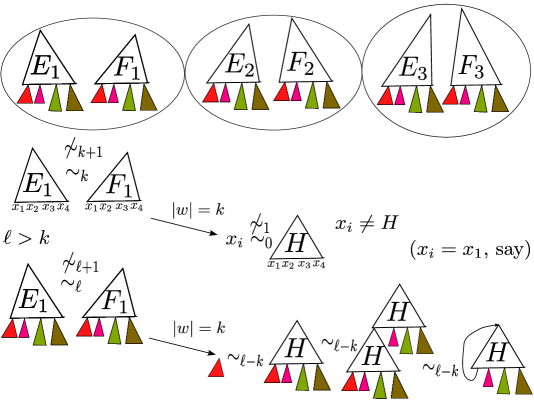
Figure 3: In an $(n,s,g)$-sequence, $(E_{1},F_{1})$ helps to get rid of one term in the tail-substitution $\sigma$

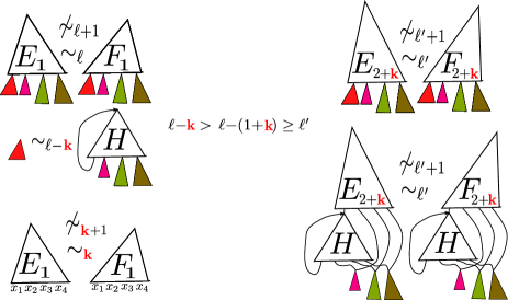
Figure 4: Support of $\sigma$ can be safely decreased after the eq-level drops sufficiently

4 Bounding the Lengths of “$(n,s,g)$-sequences”

The top of Figure 3 depicts (a prefix of) a sequence of the form

$(E_{1}\sigma,F_{1}\sigma)$, $(E_{2}\sigma,F_{2}\sigma)$, $\dots$, $(E_{z}\sigma,F_{z}\sigma)$

($E_{i},F_{i}$ being regular terms) where we assume that the eq-levels are finite and decreasing:

$\omega>\textsc{el}(E_{1}\sigma,F_{1}\sigma)>\textsc{el}(E_{2}\sigma,F_{2}\sigma)>\cdots>\textsc{el}(E_{z}\sigma,F_{z}\sigma)$.

We then have $\textsc{el}(E_{1},F_{1})=k\leq\ell=\textsc{el}(E_{1}\sigma,F_{1}\sigma)$ (for some $k,\ell\in\mathbb{N}$), by Proposition 3. If $\sigma$ is the empty-support substitution, then $k=\ell$ and the sequence length $z$ is bounded by $1+k$. If $k<\ell$, then Lemma 4 yields some $x_{i}$ and $H\neq x_{i}$ ($x_{i}=x_{1}$ in Figure 3) where $x_{i}\sigma\sim_{\ell-k}H\sigma$; hence in each pair $(E_{j}\sigma,F_{j}\sigma)$ where $j\in[2+k,z]$ we can (repeatedly) replace $x_{i}\sigma$ with $H\sigma$ without changing the eq-level of the pair. This is depicted in Figure 4; since $\textsc{el}(E_{2+k}\sigma,F_{2+k}\sigma)=\ell^{\prime}<\ell-k$, the respective eq-levels do not change due to Propositions 3 and 1.

If, moreover, we are guaranteed that the size growth of $(E_{j},F_{j})$ is controlled, i.e.,

$$\textsc{Size}(E_{j},F_{j})\leq s+g\cdot(j{-}1)$$

for some fixed constants $s$ and $g$ (and $j\in[1,z]$), and $\textsc{var}(E_{j},F_{j})\subseteq\{x_{1},\dots,x_{n}\}$ for some fixed $n$ (which bounds the support of $\sigma$), then a bound on the lengths $z$ of such $(n,s,g)$-sequences is determined by the respective grammar $\mathcal{G}$ (independently of the sizes of terms $x_{i}\sigma$). This is straightforward, as we now show.

Given $n,s,g$, the number of respective pairs $(E_{1},F_{1})$ is bounded, and there is thus $e\in\mathbb{N}$ that is the largest $\textsc{el}(E_{1},F_{1})$ for such pairs (we recall that $\omega>\textsc{el}(E_{1}\sigma,F_{1}\sigma)\geq\textsc{el}(E_{1},F_{1})$); at this moment we do not claim that $e$ is computable. For each $(n,s,g)$-sequence $(E_{1}\sigma,F_{1}\sigma)$, $(E_{2}\sigma,F_{2}\sigma)$, $\dots$, $(E_{z}\sigma,F_{z}\sigma)$ where $z>1{+}e$ we have ($\textsc{el}(E_{1},F_{1})<\textsc{el}(E_{1}\sigma,F_{1}\sigma)$ and) either $E_{1}\xrightarrow{w}x_{i}$ and $F_{1}\xrightarrow{w}H$, or $E_{1}\xrightarrow{w}H$ and $F_{1}\xrightarrow{w}x_{i}$, $|w|\leq e$, for the respective $x_{i},H$ discussed above and illustrated in Figures 3 and 4; hence $\textsc{Size}(H)\leq\textsc{Size}(E_{1},F_{1})+e\cdot\textsc{SInc}$ (by Proposition 5(1)). This entails that replacing $x_{i}\sigma$ with $H^{\prime}\sigma_{[-x_{i}]}$ where $H^{\prime}=H[x_{i}/H][x_{i}/H][x_{i}/H]\cdots$ (recall Proposition 2) in the pairs $(E_{j}\sigma,F_{j}\sigma)$ for $j=1{+}e{+}1,1{+}e{+}2,\dots,z$ gives us an $(n{-}1,s^{\prime},g)$-sequence of length $z{-}(1{+}e)$, where $s^{\prime}=s+g\cdot(1{+}e)+s+e\cdot\textsc{SInc}$ (which bounds the size of terms $E_{2+e},F_{2+e}$ extended by a shared subterm $H^{\prime}$). To be precise, for the terms $E^{\prime}_{j}=E_{j}[x_{i}/H^{\prime}]$ and $F^{\prime}_{j}=F_{j}[x_{i}/H^{\prime}]$ we only have $\textsc{var}(E^{\prime}_{j},F^{\prime}_{j})\subseteq\{x_{1},\dots,x_{n}\}\smallsetminus\{x_{i}\}$, and $x_{n}$ can occur in them (when $x_{i}\neq x_{n}$). In this case we just replace $x_{n}$ with $x_{i}$ in all $E^{\prime}_{j},F^{\prime}_{j}$ ($j=1{+}e{+}1,1{+}e{+}2,\dots,z$) and use the tail-substitution $\sigma^{\prime}$ that arises from $\sigma$ by putting $x_{i}\sigma^{\prime}=x_{n}\sigma$ and $x_{n}\sigma^{\prime}=x_{n}$. An inductive argument thus establishes that there is indeed a claimed bound (on the lengths of $(n,s,g)$-sequences) determined by the grammar.

We will later show that such a bound is even computable when $\mathcal{G},n,s,g$ are given. Moreover, we will also show how to compute small $n,s,g$ to a given $\mathcal{G}$ so that the computable bound on the length of $(n,s,g)$-sequences gives us the number $\mathcal{E}$ in Theorem 7.

In the rest of this section we formalize the above ideas showing that $(n,s,g)$-sequences are bounded. In this formalization we also define the notion of $(n,s,g)$-candidates, candidates for “non-equivalence bases”; intuitively, the base $\mathcal{B}_{n,s,g}$ is intended to collect all possible “tops” $(E_{j},F_{j})$, $(E_{j}[x_{i}/H^{\prime}],F_{j}[x_{i}/H^{\prime}])$, $\dots$ from all (eqlevel-decreasing) $(n,s,g)$-sequences that undergo the above described inductive transformation.

Eqlevel-decreasing $(n,s,g)$-sequences.

We fix a grammar $\mathcal{G}=(\mathcal{N},\Sigma,\mathcal{R})$. By an eqlevel-decreasing sequence we mean a sequence $(T_{1},U_{1}),(T_{2},U_{2}),\dots,(T_{z},U_{z})$ of pairs of terms (where $z\in\mathbb{N}_{+}$) such that $\omega>\textsc{el}(T_{1},U_{1})>\textsc{el}(T_{2},U_{2})>\cdots>\textsc{el}(T_{z},U_{z})$. The length $z$ of such a sequence is obviously at most $1+\textsc{el}(T_{1},U_{1})$.

For $n,s,g\in\mathbb{N}$ we say that an eqlevel-decreasing sequence in the form

$$(E_{1}\sigma,F_{1}\sigma),(E_{2}\sigma,F_{2}\sigma),\dots,(E_{z}\sigma,F_{z}\sigma)$$ (9)

is an $(n,s,g)$-sequence if $\textsc{var}(E_{j},F_{j})\subseteq\{x_{1},\dots,x_{n}\}$ and $\textsc{Size}(E_{j},F_{j})\leq s+g\cdot(j{-}1)$ for all $j\in[1,z]$. (The size of “tops” $(E_{j},F_{j})$ is at most $s$ at the start, and $g$ bounds the “growth-rate” of tops; the terms $x_{i}\sigma$, $i\in[1,n]$, might be large but the “tail substitution” $\sigma$ is the same in all elements of the sequence.)

Candidates for (non-equivalence) bases.

To show a bound on the lengths of $(n,s,g)$-sequences in a convenient form (in Lemma 10), we introduce further notions; we start with a piece of notation. For any $n,s\in\mathbb{N}$ we put

• $\textsc{Pairs}_{\,\textsc{var}\,:\,n}=\big{\{}(E,F)\in\textsc{Terms}_{\mathcal{N}}\times\textsc{Terms}_{\mathcal{N}}\mid\textsc{var}(E,F)=\{x_{1},\dots,x_{n}\}\big{\}}$,

• $\textsc{Pairs}_{\,\textsc{size}\leq s}=\big{\{}(E,F)\in\textsc{Terms}_{\mathcal{N}}\times\textsc{Terms}_{\mathcal{N}}\mid\textsc{Size}(E,F)\leq s\big{\}}$,

• $\textsc{Pairs}_{\,n,s}=\textsc{Pairs}_{\,\textsc{var}\,:\,n}\cap\textsc{Pairs}_{\,\textsc{size}\leq s}$.

Given $n,s,g\in\mathbb{N}$, we say that $\mathcal{B}\subseteq\textsc{Terms}_{\mathcal{N}}\times\textsc{Terms}_{\mathcal{N}}$ is an $(n,s,g)$-candidate (intended to collect the tops of $(n,s,g,)$-sequences that undergo the above described inductive transformation) if the following conditions $1$–$3$ hold (in which an implicit induction on $n$ is used):

1. $\mathcal{B}\subseteq\big{(}\textsc{Pairs}_{\,\textsc{var}\,:\,0}\cup\textsc{Pairs}_{\,\textsc{var}\,:\,1}\cup\cdots\cup\textsc{Pairs}_{\,\textsc{var}\,:\,n}\big{)}\mathop{\cap}\not\sim$ .

2. $(\mathcal{B}\cap\textsc{Pairs}_{\,\textsc{var}\,:\,n})\subseteq\textsc{Pairs}_{\,\textsc{size}\leq s}$.

3. If $n>0$, then the set $\mathcal{B}^{\prime}=\mathcal{B}\smallsetminus\textsc{Pairs}_{\,\textsc{var}\,:\,n}$ is an $(n{-}1,s^{\prime},g)$-candidate where

   $$s^{\prime}=2s+g\cdot(1{+}e)+e\cdot\textsc{SInc} e=\max\big{\{}\textsc{el}(E,F)\mid(E,F)\in\mathcal{B}\cap\textsc{Pairs}_{\,\textsc{size}\leq s}\}$$ for . (10)

Every $(n,s,g)$-candidate $\mathcal{B}$ yields a bound $\mathcal{E}^{n,s,g}_{\mathcal{B}}\in\mathbb{N}_{+}$, denoted just $\mathcal{E}_{\mathcal{B}}$ when $n,s,g$ are clear from the context; in the above notation (around (10)) we define $\mathcal{E}^{n,s,g}_{\mathcal{B}}$ as follows:

if $n=0$, then $\mathcal{E}^{n,s,g}_{\mathcal{B}}=1+e$; if $n>0$, then $\mathcal{E}^{n,s,g}_{\mathcal{B}}=1+e+\mathcal{E}^{n-1,s^{\prime},g}_{\mathcal{B}^{\prime}}$.

An $(n,s,g)$-candidate $\mathcal{B}$ is full below an eq-level $\overline{e}\in\mathbb{N}\cup\{\omega\}$ if each pair $(E,F)\in\big{(}\textsc{Pairs}_{\,\textsc{var}\,:\,0}\cup\textsc{Pairs}_{\,\textsc{var}\,:\,1}\cup\cdots\cup\textsc{Pairs}_{\,\textsc{var}\,:\,n}\big{)}\mathop{\cap}\textsc{Pairs}_{\,\textsc{size}\leq s}$ such that $\textsc{el}(E,F)<\overline{e}$ belongs to $\mathcal{B}$, and, moreover, in the case $n>0$ the $(n{-}1,s^{\prime},g)$-candidate $\mathcal{B}^{\prime}$ is full below $\overline{e}$. We say that $\mathcal{B}$ is full if it is full below $\omega$ (in which case $\mathcal{B}$ contains all relevant non-equivalent pairs).

Proposition 9.

For any $n,s,g$ there is the unique full $(n,s,g)$-candidate, denoted $\mathcal{B}_{n,s,g}$.

Proof.

Given $n,s,g$, the full $(n,s,g)$-candidate $\mathcal{B}=\mathcal{B}_{n,s,g}$ is defined as follows: $\mathcal{B}\cap\textsc{Pairs}_{\,\textsc{size}\leq s}=\big{(}\textsc{Pairs}_{\,\textsc{var}\,:\,0}\cup\textsc{Pairs}_{\,\textsc{var}\,:\,1}\cup\cdots\cup\textsc{Pairs}_{\,\textsc{var}\,:\,n}\big{)}\mathop{\cap}\textsc{Pairs}_{\,\textsc{size}\leq s}\mathop{\cap}\not\sim$ and, moreover, in the case $n>0$ the set $\mathcal{B}^{\prime}=\mathcal{B}\smallsetminus\textsc{Pairs}_{\,n,s}$ is the full $(n{-}1,s^{\prime},g)$-candidate (where $s^{\prime}$ is defined as in (10)). ∎

The unique full $(n,s,g)$-candidate $\mathcal{B}_{n,s,g}$ will be also called the $(n,s,g)$-base.

The $(n,s,g)$-sequences have bounded lengths.

We show the announced bound.

Lemma 10.

If $(E_{1}\sigma,F_{1}\sigma),(E_{2}\sigma,F_{2}\sigma),\dots,(E_{z}\sigma,F_{z}\sigma)$ is an $(n,s,g)$-sequence and $\mathcal{B}$ is an $(n,s,g)$-candidate that is full below $1+\textsc{el}(E_{1}\sigma,F_{1}\sigma)$, then $z\leq\mathcal{E}_{\mathcal{B}}$; in particular, $z\leq\mathcal{E}_{\mathcal{B}_{n,s,g}}$.

Proof.

We consider an $(n,s,g)$-sequence $(E_{1}\sigma,F_{1}\sigma),(E_{2}\sigma,F_{2}\sigma),\dots,(E_{z}\sigma,F_{z}\sigma)$ as in (9), and an $(n,s,g)$-candidate $\mathcal{B}$ that is full below $1+\textsc{el}(E_{1}\sigma,F_{1}\sigma)$. Since $\omega>\textsc{el}(E_{1}\sigma,F_{1}\sigma)\geq\textsc{el}(E_{1},F_{1})$ (by Proposition 3(1)), we have $(E_{1},F_{1})\in\mathcal{B}\cap\textsc{Pairs}_{\,\textsc{size}\leq s}$. This entails

$\textsc{el}(E_{1},F_{1})=k\leq e=\max\big{\{}\textsc{el}(E,F)\mid(E,F)\in\mathcal{B}\cap\textsc{Pairs}_{\,\textsc{size}\leq s}\}$.

If $\textsc{el}(E_{1}\sigma,F_{1}\sigma)=\textsc{el}(E_{1},F_{1})=k$, which is surely the case when $n=0$ (in this case $(E_{1}\sigma,F_{1}\sigma)=(E_{1},F_{1})$), then $z\leq 1+k$, due to the required eqlevel-decreasing property of $(n,s,g)$-sequences; in this case $z\leq 1+e\leq\mathcal{E}_{\mathcal{B}}$.

We proceed inductively (on $n$), assuming $n>0$ and $\textsc{el}(E_{1}\sigma,F_{1}\sigma)=\ell>k=\textsc{el}(E_{1},F_{1})$. By Lemma 4 there is $x_{i}\in\textsc{supp}(\sigma)$, $i\in[1,n]$, and $H\neq x_{i}$ such that $E_{1}\xrightarrow{w}x_{i}$ and $F_{1}\xrightarrow{w}H$, or $E_{1}\xrightarrow{w}H$ and $F_{1}\xrightarrow{w}x_{i}$, for some $w\in\Sigma^{*}$ with $|w|\leq k$, where $x_{i}\sigma\sim_{\ell-k}H\sigma$. Hence $\sigma\sim_{\ell-k}[x_{i}/H]\sigma$, which entails that $\sigma\sim_{\ell-k}[x_{i}/H]^{j}\sigma$ for all $j\in\mathbb{N}$ (by applying Proposition 3(2) repeatedly). We can also easily check that $[x_{i}/H]^{\ell-k}\sigma\sim_{\ell-k}[x_{i}/H]^{\omega}\sigma$ (by induction on $\ell-k$), hence

$x_{i}\sigma\sim_{\ell-k}H^{\prime}\sigma_{[-x_{i}]}$ where $H^{\prime}=H[x_{i}/H][x_{i}/H][x_{i}/H]\cdots$

(We also recall Proposition 2.) We note that

$\textsc{Size}(H^{\prime})\leq\textsc{Size}(H)\leq\max\{\textsc{Size}(E_{1}),\textsc{Size}(F_{1})\}+k\cdot\textsc{SInc}\leq s+e\cdot\textsc{SInc}$

(by using Proposition 5(1)). For each $j\in[k{+}2,z]$ we now put

$(E^{\prime}_{j},F^{\prime}_{j})=(E_{j}[x_{i}/H^{\prime}],F_{j}[x_{i}/H^{\prime}])$, hence $(E^{\prime}_{j}\sigma,F^{\prime}_{j}\sigma)=(E^{\prime}_{j}\sigma_{[-x_{i}]},F^{\prime}_{j}\sigma_{[-x_{i}]})$,

and note that $\textsc{el}(E_{j}\sigma,F_{j}\sigma)=\textsc{el}(E^{\prime}_{j}\sigma_{[-x_{i}]},F^{\prime}_{j}\sigma_{[-x_{i}]})$, since $\textsc{el}(E_{j}\sigma,F_{j}\sigma)<\ell{-}k$ (for each $j\geq k{+}2$); here we use that $\textsc{el}(E_{j}\sigma,E_{j}[x_{i}/H^{\prime}]\sigma)\geq\ell{-}k$ and $\textsc{el}(F_{j}\sigma,F_{j}[x_{i}/H^{\prime}]\sigma)\geq\ell{-}k$, and we recall Proposition 1(1). We also note that for each $j\in[k{+}2,z]$ we have

$\textsc{Size}(E^{\prime}_{j},F^{\prime}_{j})\leq\textsc{Size}(E_{j},F_{j})+\textsc{Size}(H^{\prime})\leq s+g\cdot(j{-}1)+s+e\cdot\textsc{SInc}=2s+g\cdot(j{-}1)+e\cdot\textsc{SInc}$.

Hence $\textsc{Size}(E^{\prime}_{k+2},F^{\prime}_{k+2})\leq 2s+g\cdot(1+k)+e\cdot\textsc{SInc}\leq 2s+g\cdot(1+e)+e\cdot\textsc{SInc}=s^{\prime}$ (recall $s^{\prime}$ from (10)). Thus the sequence

$(E^{\prime}_{k{+}2}\sigma_{[-x_{i}]},F^{\prime}_{k+2}\sigma_{[-x_{i}]})$, $(E^{\prime}_{k{+}3}\sigma_{[-x_{i}]},F^{\prime}_{k+3}\sigma_{[-x_{i}]})$$\dots$, $(E^{\prime}_{z}\sigma_{[-x_{i}]},F^{\prime}_{z}\sigma_{[-x_{i}]})$

is “almost” an $(n{-}1,s^{\prime},g)$-sequence. The only problem is that $x_{n}$ can occur in $E^{\prime}_{j},F^{\prime}_{j}$. But we use the fact that $x_{i}$ does not occur in $E^{\prime}_{j},F^{\prime}_{j}$, and we replace $x_{n}$ with $x_{i}$, while replacing $\sigma_{[-x_{i}]}$ with $\sigma^{\prime}$ where $x_{n}\sigma^{\prime}=x_{n}$, $x_{i}\sigma^{\prime}=x_{n}\sigma_{[-x_{i}]}$, and $x\sigma^{\prime}=x\sigma_{[-x_{i}]}$ for all $x\in\textsc{Var}\smallsetminus\{x_{i},x_{n}\}$.

We note that the $(n{-}1,s^{\prime},g)$-candidate $\mathcal{B}^{\prime}=\mathcal{B}\smallsetminus\textsc{Pairs}_{\,\textsc{var}\,:\,n}$ is full below $1+\textsc{el}(E^{\prime}_{k+2}\sigma_{[-x_{i}]},F^{\prime}_{k+2}\sigma_{[-x_{i}]})$ (since $\mathcal{B}^{\prime}$ is full below $1+\textsc{el}(E_{1}\sigma,F_{1}\sigma)$, and $\textsc{el}(E^{\prime}_{k+2}\sigma_{[-x_{i}]},F^{\prime}_{k+2}\sigma_{[-x_{i}]})=\textsc{el}(E_{k+2}\sigma,F_{k+2}\sigma)<\textsc{el}(E_{1}\sigma,F_{1}\sigma)$). By the induction hypothesis $z{-}(k{+}1)\leq\mathcal{E}_{\mathcal{B}^{\prime}}$, and thus $z\leq 1{+}k{+}\mathcal{E}_{\mathcal{B}^{\prime}}\leq 1{+}e{+}\mathcal{E}_{\mathcal{B}^{\prime}}=\mathcal{E}_{\mathcal{B}}$. ∎

In the final argument of the proof of Theorem 7 (in Section 7) we will use $\mathcal{E}_{\mathcal{B}_{n,s,g}}$ as $\mathcal{E}$ in (8), for some specific small $n,s,g$. Though we have defined the $(n,s,g)$-base $\mathcal{B}_{n,s,g}$ only semantically, it will turn out that it coincides with an effectively constructible “sound” $(n,s,g)$-candidate. But we first need some further technicalities to clarify the specific $n,s,g$ (as well as $c$ in (8)).

5 Plays (of Bisimulation Game) and their Balancing

In Section 1 we discussed the notion of optimal plays, which we make more precise now. We assume a given grammar $\mathcal{G}=(\mathcal{N},\Sigma,\mathcal{R})$; for $r\in\mathcal{R}$ of the form $A(x_{1},\dots,x_{m})\xrightarrow{a}E$ we put $\textsc{lab}(r)=a$. For technical convenience, by a play we only mean an optimal play from a non-equivalent pair, i.e., a sequence

$$\overset{T_{0}}{\underset{U_{0}}{}}\overset{r_{1}}{\underset{r^{\prime}_{1}}{\longrightarrow}}\overset{T_{1}}{\underset{U_{1}}{}}\overset{r_{2}}{\underset{r^{\prime}_{2}}{\longrightarrow}}\overset{T_{2}}{\underset{U_{2}}{}}\cdots\overset{r_{k}}{\underset{r^{\prime}_{k}}{\longrightarrow}}\overset{T_{k}}{\underset{U_{k}}{}}$$ (11)

where for each $i\in[1,k]$ we have $r_{i},r^{\prime}_{i}\in\mathcal{R}$, $\textsc{lab}(r_{i})=\textsc{lab}(r^{\prime}_{i})$, $T_{i-1}\xrightarrow{r_{i}}T_{i}$, $U_{i-1}\xrightarrow{r^{\prime}_{i}}U_{i}$ (in the LTS $\mathcal{L}^{\textsc{r}}_{\mathcal{G}}$); moreover, $\omega>\textsc{el}(T_{0},U_{0})$ and $\textsc{el}(T_{i},U_{i})=\textsc{el}(T_{i-1},U_{i-1})-1$ for each $i\in[1,k]$ (in the LTS $\mathcal{L}^{\textsc{a}}_{\mathcal{G}}$). If $\textsc{el}(T_{k},E_{k})=0$, then it is a completed play, in which case $\textsc{el}(T_{0},U_{0})=k$. (We recall that $T_{0},U_{0}$ can be regular terms of a large size.) The length of the play (11) is (defined to be) $k$, and another presentation of the play is $\overset{T_{0}}{\underset{U_{0}}{}}\overset{u}{\underset{u^{\prime}}{\longrightarrow}}\overset{T_{k}}{\underset{U_{k}}{}}$, or also just $\overset{T_{0}}{\underset{U_{0}}{}}\overset{u}{\underset{u^{\prime}}{\longrightarrow}}$, where $u=r_{1}r_{2}\cdots r_{k}$ and $u^{\prime}=r^{\prime}_{1}r^{\prime}_{2}\cdots r^{\prime}_{k}$.

Our aim is to bound the lengths of completed plays in the way stated in Theorem 7. To facilitate this task, in this section we show a particular transformation of a completed play (11) into a sequence of plays of the same overall length (i.e., the sum of lengths) that are connected by so-called eqlevel-concatenation $\odot$; such concatenation

$$\left[\overset{T}{\underset{U}{}}\overset{u_{1}}{\underset{u^{\prime}_{1}}{\longrightarrow}}\overset{T^{\prime}}{\underset{U^{\prime}}{}}\right]\odot\left[\overset{T^{\prime\prime}}{\underset{U^{\prime\prime}}{}}\overset{u_{2}}{\underset{u^{\prime}_{2}}{\longrightarrow}}\overset{T^{\prime\prime\prime}}{\underset{U^{\prime\prime\prime}}{}}\right]$$

is defined if (and only if) $\textsc{el}(T^{\prime},U^{\prime})=\textsc{el}(T^{\prime\prime},U^{\prime\prime})$, though the pairs $(T^{\prime},U^{\prime})$ and $(T^{\prime\prime},U^{\prime\prime})$ can differ. The overall length of this concatenation is $|u_{1}|+|u_{2}|$; if $\overset{T^{\prime\prime}}{\underset{U^{\prime\prime}}{}}\overset{u_{2}}{\underset{u^{\prime}_{2}}{\longrightarrow}}\overset{T^{\prime\prime\prime}}{\underset{U^{\prime\prime\prime}}{}}$ is a completed play, then this length ($|u_{1}|+|u_{2}|$) is obviously the same as the length of any completed play starting with $(T,U)$.

In the first phase of the mentioned transformation of a completed play (11) we will replace it with the concatenation of two plays in the form

$$\left[\overset{T_{0}}{\underset{U_{0}}{}}\overset{v_{0}u_{1}}{\underset{v^{\prime}_{0}u^{\prime}_{1}}{\longrightarrow}}\overset{T^{\prime}_{1}}{\underset{U^{\prime}_{1}}{}}\right]\odot\left[\overset{T^{\prime\prime}_{1}}{\underset{U^{\prime\prime}_{1}}{}}\overset{v}{\underset{v^{\prime}}{\longrightarrow}}\right]$$

where $v_{0}u_{1}$ is a certain prefix of $u=r_{1}r_{2}\cdots r_{k}$, $v^{\prime}_{0}u^{\prime}_{1}$ is a prefix of $u^{\prime}=r^{\prime}_{1}r^{\prime}_{2}\cdots r^{\prime}_{k}$ (of the same length as $v_{0}u_{1}$), and $\left[\overset{T^{\prime\prime}_{1}}{\underset{U^{\prime\prime}_{1}}{}}\overset{v}{\underset{v^{\prime}}{\longrightarrow}}\right]$ is a completed play (while $v$ ($v^{\prime}$) is generally not a suffix of $u$ ($u^{\prime}$)). Further we replace $\left[\overset{T^{\prime\prime}_{1}}{\underset{U^{\prime\prime}_{1}}{}}\overset{v}{\underset{v^{\prime}}{\longrightarrow}}\right]$ with $\left[\overset{T^{\prime\prime}_{1}}{\underset{U^{\prime\prime}_{1}}{}}\overset{v_{1}u_{2}}{\underset{v^{\prime}_{1}u^{\prime}_{2}}{\longrightarrow}}\overset{T^{\prime}_{2}}{\underset{U^{\prime}_{2}}{}}\right]\odot\left[\overset{T^{\prime\prime}_{2}}{\underset{U^{\prime\prime}_{2}}{}}\overset{\bar{v}}{\underset{\bar{v}^{\prime}}{\longrightarrow}}\right]$ where $v_{1}u_{2}$ is a certain prefix of $v$, $v^{\prime}_{1}u^{\prime}_{2}$ is a prefix of $v^{\prime}$, and $\left[\overset{T^{\prime\prime}_{2}}{\underset{U^{\prime\prime}_{2}}{}}\overset{\bar{v}}{\underset{\bar{v}^{\prime}}{\longrightarrow}}\right]$ is a completed play; we continue in this way, doing $\ell$ phases for a certain number $\ell$, until finally getting

$$\left[\overset{T_{0}}{\underset{U_{0}}{}}\overset{v_{0}}{\underset{v^{\prime}_{0}}{\longrightarrow}}\overset{\bar{T}_{1}}{\underset{\bar{U}_{1}}{}}\overset{u_{1}}{\underset{u^{\prime}_{1}}{\longrightarrow}}\overset{T^{\prime}_{1}}{\underset{U^{\prime}_{1}}{}}\right]\odot\left[\overset{T^{\prime\prime}_{1}}{\underset{U^{\prime\prime}_{1}}{}}\overset{v_{1}}{\underset{v^{\prime}_{1}}{\longrightarrow}}\overset{\bar{T}_{2}}{\underset{\bar{U}_{2}}{}}\overset{u_{2}}{\underset{u^{\prime}_{2}}{\longrightarrow}}\overset{T^{\prime}_{2}}{\underset{U^{\prime}_{2}}{}}\right]\odot\left[\overset{T^{\prime\prime}_{2}}{\underset{U^{\prime\prime}_{2}}{}}\overset{v_{2}}{\underset{v^{\prime}_{2}}{\longrightarrow}}\cdots\cdots\overset{\bar{T}_{\ell}}{\underset{\bar{U}_{\ell}}{}}\overset{u_{\ell}}{\underset{u^{\prime}_{\ell}}{\longrightarrow}}\overset{T^{\prime}_{\ell}}{\underset{U^{\prime}_{\ell}}{}}\right]\odot\left[\overset{T^{\prime\prime}_{\ell}}{\underset{U^{\prime\prime}_{\ell}}{}}\overset{v_{\ell}}{\underset{v^{\prime}_{\ell}}{\longrightarrow}}\overset{\bar{T}_{\ell+1}}{\underset{\bar{U}_{\ell+1}}{}}\right]$$ (12)

where $\left[\overset{T^{\prime\prime}_{\ell}}{\underset{U^{\prime\prime}_{\ell}}{}}\overset{v_{\ell}}{\underset{v^{\prime}_{\ell}}{\longrightarrow}}\overset{\bar{T}_{\ell+1}}{\underset{\bar{U}_{\ell+1}}{}}\right]$ is completed and “non-transformable”; the overall length of (12) is thus equal to $k=\textsc{el}(T_{0},U_{0})$. In fact, we have $\ell=0$ when already (11) is non-transformable; we thus put $(T^{\prime\prime}_{0},U^{\prime\prime}_{0})=(T_{0},U_{0})$ for convenience. (Later we repeat (12) as (17) without the bars in the notation $\bar{T}_{j},\bar{U}_{j}$; now the bars are added to avoid the confusion with ${T}_{j},{U}_{j}$ in (11).)

More concretely, we will perform the transformation so that for each phase $j\in[1,\ell]$ we have $|u_{j}|=d_{0}$ (for $d_{0}$ defined by (6)), one of the terms $\bar{T}_{j},\bar{U}_{j}$ is the pivot $W_{j}$, and the pair $(T^{\prime\prime}_{j},U^{\prime\prime}_{j})$ is the balancing result, or the bal-result for short, related to the pivot $W_{j}$.

In fact, if $W_{j}=\bar{U}_{j}$, then we have $U^{\prime\prime}_{j}=U^{\prime}_{j}$ (and $T^{\prime\prime}_{j}\neq T^{\prime}_{j}$); in this case the $j$-th phase consists in replacing the completed play $\left[\overset{T^{\prime\prime}_{j-1}}{\underset{U^{\prime\prime}_{j-1}}{}}\overset{v}{\underset{v^{\prime}}{\longrightarrow}}\right]$ with the eqlevel-concatenation $\left[\overset{T^{\prime\prime}_{j-1}}{\underset{U^{\prime\prime}_{j-1}}{}}\overset{v_{j-1}}{\underset{v^{\prime}_{j-1}}{\longrightarrow}}\overset{\bar{T}_{j}}{\underset{\bar{U}_{j}}{}}\overset{u_{j}}{\underset{u^{\prime}_{j}}{\longrightarrow}}\overset{T^{\prime}_{j}}{\underset{U^{\prime}_{j}}{}}\right]\odot\left[\overset{T^{\prime\prime}_{j}}{\underset{U^{\prime}_{j}}{}}\overset{\bar{v}}{\underset{\bar{v}^{\prime}}{\longrightarrow}}\right]$ (where $\left[\overset{T^{\prime\prime}_{j-1}}{\underset{U^{\prime\prime}_{j-1}}{}}\overset{v_{j-1}}{\underset{v^{\prime}_{j-1}}{\longrightarrow}}\overset{\bar{T}_{j}}{\underset{\bar{U}_{j}}{}}\overset{u_{j}}{\underset{u^{\prime}_{j}}{\longrightarrow}}\overset{T^{\prime}_{j}}{\underset{U^{\prime}_{j}}{}}\right]$ is a prefix of $\left[\overset{T^{\prime\prime}_{j-1}}{\underset{U^{\prime\prime}_{j-1}}{}}\overset{v}{\underset{v^{\prime}}{\longrightarrow}}\right]$); this is called a left balancing step (the left term in $(T^{\prime}_{j},U^{\prime}_{j})$ has been replaced with $T^{\prime\prime}_{j}$ so that $\textsc{el}(T^{\prime}_{j},U^{\prime}_{j})=\textsc{el}(T^{\prime\prime}_{j},U^{\prime}_{j})$). Similarly, if $W_{j}=\bar{T}_{j}$, then we have $T^{\prime\prime}_{j}=T^{\prime}_{j}$, and we have performed a right balancing step, replacing $U^{\prime}_{j}$ with $U^{\prime\prime}_{j}$.

We thus have pivots $W_{1},W_{2},\dots,W_{\ell}$, each having its related bal-result. Since the sequence

$(T^{\prime\prime}_{1},U^{\prime\prime}_{1}),(T^{\prime\prime}_{2},U^{\prime\prime}_{2}),\dots,(T^{\prime\prime}_{\ell},U^{\prime\prime}_{\ell})$

of bal-results is eqlevel-decreasing, no pair can repeat in the sequence.

We will “balance” in a way that will also yield a pivot path

$$W_{0}\xrightarrow{w_{0}}W_{1}\xrightarrow{w_{1}}W_{2}\xrightarrow{w_{2}}\cdots W_{\ell}\xrightarrow{w_{\ell}}W_{\ell+1}$$ (13)

where $w_{0}\in\mathcal{R}^{*}$, $w_{j}\in\mathcal{R}^{+}$ for $j\in[1,\ell]$, $W_{0}\in\{T_{0},U_{0}\}$, $W_{\ell+1}\in\{\bar{T}_{\ell+1},\bar{U}_{\ell+1}\}$, and we will guarantee the following properties:

1. There is some small $n$ such that for each $j\in[1,\ell]$ there are small finite terms $G,E,F$, with $\textsc{var}(E,F)\subseteq\textsc{var}(G)\subseteq\{x_{1},\dots,x_{n}\}$, such that

   $W_{j}=G\sigma$ and $(T^{\prime\prime}_{j},U^{\prime\prime}_{j})=(E\sigma,F\sigma)$,

   for a substitution $\sigma$ (with $\textsc{supp}(\sigma)\subseteq\{x_{1},\dots,x_{n}\}$). (Hence the terms in the bal-result arise from the pivot $W$ by replacing a small top of $W$ by other small tops.) This is depicted in Figure 5 for some $W_{j}$ and $W_{j+1}$ (and in more detail in Figure 6).

2. Each pivot-path segment $W_{j}\xrightarrow{w_{j}}W_{j+1}$ (for $j\in[0,\ell]$) is either short (i.e., its length is small), or it has a short prefix and a short suffix while the middle part is “quickly sinking” (to a deep subterm of $W_{j}$ if this part is long).

We note that we do not exclude that a pivot $W$ occurs more than once in the pivot path ($W=W_{j}$ and $W=W_{j^{\prime}}$ for $j\neq j^{\prime}$), but the number of its occurrences must be small; this follows from the point $1$ which entails that there is only a small number of possible bal-results related to one pivot, and from the fact that the bal-results cannot repeat.

Figure 5 depicts a “non-sinking segment” on the pivot path. (In such a segment, no root-successor of the starting term is exposed.) By the above point $2$ it is intuitively clear that any long non-sinking segment must contain a large number of pivots, and that the possible increase of (the tops of) the pivots is controlled. Hence any long non-sinking segment of the pivot path gives rise to a long $(n,s,g)$-sequence, for some small $n,s,g$; here we use the point $1$ (and recall Figure 5). This is a crucial fact for our proof of Theorem 7.

In this section, our task is to show a transformation that guarantees a suitable pivot path (13) and the above properties $1$ and $2$.

A concrete way how we do a left balancing step is captured by Figure 6. Informally speaking, if the left-hand side does not sink to a root-successor within less than $d_{0}$ moves (for $d_{0}$ defined by (6)), which is the case in Figure 6 due to $A(x_{1},\dots,x_{m})\xrightarrow{u}E^{\prime}$, then the other side ($U=G\sigma$ in Figure 6) can become a pivot, and the bal-result can be created as depicted; the original root-successors in the left-hand side are replaced by suitable terms that are shortly reachable from the pivot, so that the respective eq-level does not change ($\textsc{el}(E^{\prime}\sigma^{\prime},U^{\prime})=\textsc{el}(E^{\prime}\sigma^{\prime\prime},U^{\prime})$ in Figure 6). The existence of such a transformation (we claim nothing about its effectiveness) is clear by Propositions 1 and 3. Right balancing steps are analogous (they are elligible when the right-hand side does not sink within less than $d_{0}$ moves).

We observe that any path $W\xrightarrow{v}W^{\prime}$ can sink to some depth-$|v|$ subterm of $W$ at most, surely not deeper; hence $W^{\prime}$ arises from $W$ by replacing its “$|v|$-top” with another top; the size of these tops is small when $v$ is short. This observation now easily entails the above property $1$, guaranteed by our transformation.

To guarantee a suitable pivot path (13) and its property $2$, as a first attempt we consider the following procedure in the $j$-th phase (of the transformation of (11) into (12)): when we are about to replace the completed play $\left[\overset{T^{\prime\prime}_{j-1}}{\underset{U^{\prime\prime}_{j-1}}{}}\overset{v}{\underset{v^{\prime}}{\longrightarrow}}\right]$, we use its shortest prefix of the form $\left[\overset{T^{\prime\prime}_{j-1}}{\underset{U^{\prime\prime}_{j-1}}{}}\overset{v_{j-1}}{\underset{v^{\prime}_{j-1}}{\longrightarrow}}\overset{\bar{T}_{j}}{\underset{\bar{U}_{j}}{}}\overset{u_{j}}{\underset{u^{\prime}_{j}}{\longrightarrow}}\overset{T^{\prime}_{j}}{\underset{U^{\prime}_{j}}{}}\right]$ where $\left[\overset{\bar{T}_{j}}{\underset{\bar{U}_{j}}{}}\overset{u_{j}}{\underset{u^{\prime}_{j}}{\longrightarrow}}\overset{T^{\prime}_{j}}{\underset{U^{\prime}_{j}}{}}\right]$ enables a (left or right) balancing step (i.e., some side does not sink to a root successor within less than $d_{0}$ moves).

But doing this balancing as suggested would complicate our task of creating a suitable pivot path (13), as we now discuss. First we note that we can smoothly define $W_{0}\xrightarrow{w_{0}}W_{1}$: it is $U_{0}\xrightarrow{v_{0}}U_{1}$ if $W_{1}=U_{1}$, and $T_{0}\xrightarrow{v_{0}}T_{1}$ if $W_{1}=T_{1}$. Similarly we define $W_{\ell}\xrightarrow{w_{\ell}}W_{\ell+1}$ as $\bar{U}_{\ell}\xrightarrow{u^{\prime}_{\ell}v^{\prime}_{\ell}}\bar{U}_{\ell+1}$ if $W_{\ell}=\bar{U}_{\ell}$, and as $\bar{T}_{\ell}\xrightarrow{u_{\ell}v_{\ell}}\bar{T}_{\ell+1}$ if $W_{\ell}=\bar{T}_{\ell}$. If in the consecutive phases $j$ and $j{+}1$ we have the pivot on the same side, say $W_{j}=\bar{U}_{j}$ and $W_{j+1}=\bar{U}_{j+1}$, then we have no problem either: we define $W_{j}\xrightarrow{w_{j}}W_{j+1}$ simply as $\bar{U}_{j}\xrightarrow{u^{\prime}_{j}v^{\prime}_{j}}\bar{U}_{j+1}$ (which is legal since $U^{\prime}_{j}=U^{\prime\prime}_{j}$).

A problem to define $W_{j}\xrightarrow{w_{j}}W_{j+1}$ arises when there is a switch of balancing sides. Hence we add a simple condition to be satisfied when such a switch is allowed to occur. Suppose $W_{j}=U_{j}$, and let Figure 6 describe the respective left balancing step. In the $(j{+}1)$-th phase of the transformation we have

$\left[\overset{T_{0}}{\underset{U_{0}}{}}\overset{v_{0}}{\underset{v^{\prime}_{0}}{\longrightarrow}}\overset{\bar{T}_{1}}{\underset{\bar{U}_{1}}{}}\overset{u_{1}}{\underset{u^{\prime}_{1}}{\longrightarrow}}\overset{T^{\prime}_{1}}{\underset{U^{\prime}_{1}}{}}\right]\odot\cdots\odot\left[\overset{T^{\prime\prime}_{j-1}}{\underset{U^{\prime\prime}_{j-1}}{}}\overset{v_{j-1}}{\underset{v^{\prime}_{j-1}}{\longrightarrow}}\overset{\bar{T}_{j}}{\underset{W_{j}}{}}\overset{u_{j}}{\underset{u^{\prime}_{j}}{\longrightarrow}}\overset{E^{\prime}\sigma^{\prime}}{\underset{U^{\prime}_{j}}{}}\right]\odot\left[\overset{E^{\prime}\sigma^{\prime\prime}}{\underset{U^{\prime}_{j}}{}}\overset{v}{\underset{v^{\prime}}{\longrightarrow}}\right]$

and we are about to replace the (current) completed play $\left[\overset{E^{\prime}\sigma^{\prime\prime}}{\underset{U^{\prime}_{j}}{}}\overset{v}{\underset{v^{\prime}}{\longrightarrow}}\right]$. We would prefer to do another left balancing, ideally for a short prefix of this completed play. This is not possible only if the path $E^{\prime}\sigma^{\prime\prime}\xrightarrow{v}$ is quickly sinking in the beginning, i.e., within each segment of length $d_{0}$ a root-successor of the term starting the segment is exposed; the path $E^{\prime}\sigma^{\prime\prime}\xrightarrow{v}$ thus has a short prefix $E^{\prime}\sigma^{\prime\prime}\xrightarrow{v_{j1}}x_{i}\sigma^{\prime\prime}$ for some $x_{i}$ (since $E^{\prime}$ is a small finite term and the path sinks along one of its branches). But $x_{i}\sigma^{\prime\prime}$ is reachable from the last pivot $W_{j}$ ($W_{j}=U_{j}$) by a short word $\bar{v}$ (e.g., if $x_{i}\sigma^{\prime\prime}=V_{2}$ in Figure 6, then we use the path $U\xrightarrow{\bar{v}_{2}}V_{2}$). Hence only after such a short prefix $\left[\overset{E^{\prime}\sigma^{\prime\prime}}{\underset{U^{\prime}_{j}}{}}\overset{v_{j1}}{\underset{v^{\prime}_{j1}}{\longrightarrow}}\overset{x_{i}\sigma^{\prime\prime}}{\underset{\overline{U}}{}}\right]$ we allow to balance on both sides (if a left balancing is not possible earlier).

If a switch of balancing sides indeed happens in our discussed case, then we can write the $j$-th and the $(j{+}1)$-th play in the sequence (12) in the form

$\left[\overset{T^{\prime\prime}_{j-1}}{\underset{U^{\prime\prime}_{j-1}}{}}\overset{v_{j-1}}{\underset{v^{\prime}_{j-1}}{\longrightarrow}}\overset{\bar{T}_{j}}{\underset{W_{j}}{}}\overset{u_{j}}{\underset{u^{\prime}_{j}}{\longrightarrow}}\overset{E^{\prime}\sigma^{\prime}}{\underset{U^{\prime}_{j}}{}}\right]\odot\left[\overset{E^{\prime}\sigma^{\prime\prime}}{\underset{U^{\prime}_{j}}{}}\overset{v_{j1}}{\underset{v^{\prime}_{j1}}{\longrightarrow}}\overset{x_{i}\sigma^{\prime\prime}}{\underset{\overline{U}}{}}\overset{v_{j2}}{\underset{v^{\prime}_{j2}}{\longrightarrow}}\overset{W_{j+1}}{\underset{\bar{U}_{j+1}}{}}\overset{u_{j+1}}{\underset{u^{\prime}_{j+1}}{\longrightarrow}}\overset{T^{\prime}_{j+1}}{\underset{U^{\prime}_{j+1}}{}}\right]$

and define $W_{j}\xrightarrow{w_{j}}W_{j+1}$ as $W_{j}\xrightarrow{\bar{v}}x_{i}\sigma^{\prime\prime}\xrightarrow{v_{j_{2}}}W_{j+1}$ (where $\bar{v}$ is shorter than the short word $u_{j}v_{j1}$ but this does not matter). To summarize: for the consecutive phases $j$ and $j{+}1$ where the $j$-th phase is a left-balancing step captured by Figure 6, we get

$\left[\overset{T^{\prime\prime}_{j-1}}{\underset{U^{\prime\prime}_{j-1}}{}}\overset{v_{j-1}}{\underset{v^{\prime}_{j-1}}{\longrightarrow}}\overset{\bar{T}_{j}}{\underset{W_{j}}{}}\overset{u_{j}}{\underset{u^{\prime}_{j}}{\longrightarrow}}\overset{E^{\prime}\sigma^{\prime}}{\underset{U^{\prime}_{j}}{}}\right]\odot\left[\overset{E^{\prime}\sigma^{\prime\prime}}{\underset{U^{\prime}_{j}}{}}\overset{v_{j}}{\underset{v^{\prime}_{j}}{\longrightarrow}}\overset{\bar{T}_{j+1}}{\underset{\bar{U}_{j+1}}{}}\overset{u_{j+1}}{\underset{u^{\prime}_{j+1}}{\longrightarrow}}\overset{T^{\prime}_{j+1}}{\underset{U^{\prime}_{j+1}}{}}\right]$

where either $v_{j}$ is short and $W_{j+1}=\bar{U}_{j+1}$ or we can write $v_{j}=v_{j1}v_{j2}$ where $v_{j1}$ is short and we have $E^{\prime}\sigma^{\prime\prime}\xrightarrow{v_{j1}}x_{i}\sigma^{\prime\prime}$. In the latter case we can write

$$\left[\overset{E^{\prime}\sigma^{\prime\prime}}{\underset{U^{\prime}_{j}}{}}\overset{v_{j}}{\underset{v^{\prime}_{j}}{\longrightarrow}}\overset{\bar{T}_{j+1}}{\underset{\bar{U}_{j+1}}{}}\overset{u_{j+1}}{\underset{u^{\prime}_{j+1}}{\longrightarrow}}\overset{T^{\prime}_{j+1}}{\underset{U^{\prime}_{j+1}}{}}\right]=\left[\overset{E^{\prime}\sigma^{\prime\prime}}{\underset{U^{\prime}_{j}}{}}\overset{v_{j1}}{\underset{v^{\prime}_{j1}}{\longrightarrow}}\overset{x_{i}\sigma^{\prime\prime}}{\underset{\overline{U}}{}}\overset{v_{j2}}{\underset{v^{\prime}_{j2}}{\longrightarrow}}\overset{\bar{T}_{j+1}}{\underset{\bar{U}_{j+1}}{}}\overset{u_{j+1}}{\underset{u^{\prime}_{j+1}}{\longrightarrow}}\overset{T^{\prime}_{j+1}}{\underset{U^{\prime}_{j+1}}{}}\right]$$ (14)

where $W_{j+1}\in\{\bar{T}_{j+1},\bar{U}_{j+1}\}$, and both paths $x_{i}\sigma^{\prime\prime}\xrightarrow{v_{j2}}\bar{T}_{j+1}$ and $\bar{U}\xrightarrow{v^{\prime}_{j2}}\bar{U}_{j+1}$ (that may be long) are quickly sinking (since there is no balancing possibility there).

Hence the above property $2$ of the pivot path is also clear (including the case $W_{j+1}=\bar{U}_{j+1}$, where $W_{j}\xrightarrow{w_{j}}W_{j+1}$ is $\bar{U}_{j}\xrightarrow{u^{\prime}_{j}v^{\prime}_{j1}v^{\prime}_{j2}}\bar{U}_{j+1}$).

Now we define the described transformation in a more formal way.

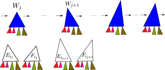
Figure 5: Non-sinking segment on the pivot path gives rise to an $(n,s,g)$-sequence

Modified optimal plays, and their eqlevel-concatenation.

We still assume a fixed grammar $\mathcal{G}=(\mathcal{N},\Sigma,\mathcal{R})$. Now we let $u,v,w$ (with subscripts etc.) range over $\mathcal{R}^{*}$ (not over $\Sigma^{*}$); hence $E\xrightarrow{w}F$ determines one path in the LTS $\mathcal{L}^{\textsc{r}}_{\mathcal{G}}$. For $r\in\mathcal{R}$ of the form $A(x_{1},\dots,x_{m})\xrightarrow{a}E$ we put $\textsc{lab}(r)=a$; this is extended to the respective homomorphism $\textsc{lab}:\mathcal{R}^{*}\rightarrow\Sigma^{*}$.

An optimal play, or just a play for short, is a sequence

$(T_{0},U_{0})(r_{1},r^{\prime}_{1})(T_{1},U_{1})(r_{2},r^{\prime}_{2})(T_{2},U_{2})\cdots(r_{k},r^{\prime}_{k})(T_{k},U_{k})$,

denoted as

$$\overset{T_{0}}{\underset{U_{0}}{}}\overset{r_{1}}{\underset{r^{\prime}_{1}}{\longrightarrow}}\overset{T_{1}}{\underset{U_{1}}{}}\overset{r_{2}}{\underset{r^{\prime}_{2}}{\longrightarrow}}\overset{T_{2}}{\underset{U_{2}}{}}\cdots\overset{r_{k}}{\underset{r^{\prime}_{k}}{\longrightarrow}}\overset{T_{k}}{\underset{U_{k}}{}}$$ , (15)

where $T_{0}\not\sim U_{0}$ and for each $j\in[1,k]$ we have $T_{j-1}\xrightarrow{r_{j}}T_{j}$, $U_{j-1}\xrightarrow{r^{\prime}_{j}}U_{j}$, $\textsc{lab}(r_{j})=\textsc{lab}(r^{\prime}_{j})$, and $\textsc{el}(T_{j},U_{j})=\textsc{el}(T_{j-1},U_{j-1})-1$. It is clear (by Proposition 1(2,3)) that for any $T_{0}\not\sim U_{0}$ there is a play of the form (15) such that $k=\textsc{el}(T_{0},U_{0})$ (and $\textsc{el}(T_{k},U_{k})=0$).

A play $\mu$ of the form (15) is a play from $\textsc{Start}(\mu)=(T_{0},U_{0})$ to $\textsc{End}(\mu)=(T_{k},U_{k})$, and is also written as $\overset{T_{0}}{\underset{U_{0}}{}}\overset{u}{\underset{u^{\prime}}{\longrightarrow}}\overset{T_{k}}{\underset{U_{k}}{}}$, or just as $\overset{T_{0}}{\underset{U_{0}}{}}\overset{u}{\underset{u^{\prime}}{\longrightarrow}}$, where $u=r_{1}r_{2}\cdots r_{k}$ and $u^{\prime}=r^{\prime}_{1}r^{\prime}_{2}\cdots r^{\prime}_{k}$; we put $\textsc{length}(\mu)=k$ and $\textsc{Pairs}(\mu)=\{(T_{i},U_{i})\mid i\in[0,k]\}$. We also consider the trivial plays of the form $(T_{0},U_{0})$ with the length $k=0$ (for $T_{0}\not\sim U_{0}$). A play (15) is a completed play if $\textsc{el}(T_{k},U_{k})=0$.

The standard concatenation $\mu\nu$ of plays $\mu=\overset{T}{\underset{U}{}}\overset{u}{\underset{u^{\prime}}{\longrightarrow}}\overset{T^{\prime}}{\underset{U^{\prime}}{}}$ and $\nu=\overset{T^{\prime\prime}}{\underset{U^{\prime\prime}}{}}\overset{v}{\underset{v^{\prime}}{\longrightarrow}}\overset{T^{\prime\prime\prime}}{\underset{U^{\prime\prime\prime}}{}}$ is defined if (and only if) $(T^{\prime},U^{\prime})=(T^{\prime\prime},U^{\prime\prime})$; in this case $\mu\nu$ is the play $\overset{T}{\underset{U}{}}\overset{uv}{\underset{u^{\prime}v^{\prime}}{\longrightarrow}}\overset{T^{\prime\prime\prime}}{\underset{U^{\prime\prime\prime}}{}}$ (hence $\textsc{End}(\mu)$ and $\textsc{Start}(\nu)$ get merged).

We aim to show a bound of the form (8) on the lengths of completed plays from $(T,U)$. The use of $(n,s,g)$-sequences, bounded by Lemma 10, will become clear after we introduce a special modification of plays. Generally,

a modified play $\pi$ is a sequence of plays $\mu_{1},\mu_{2},\ldots,\mu_{\ell}$ ($\ell\geq 1$)

where for each $j\in[1,\ell{-}1]$ we have $\textsc{el}(\textsc{End}(\mu_{j}))=\textsc{el}(\textsc{Start}(\mu_{j+1}))$ but $\textsc{End}(\mu_{j})\neq\textsc{Start}(\mu_{j+1})$; it is a modified play from $\textsc{Start}(\pi)=\textsc{Start}(\mu_{1})$ to $\textsc{End}(\pi)=\textsc{End}(\mu_{\ell})$, and it is a completed modified play if $\textsc{el}(\textsc{End}(\mu_{\ell}))=0$. (As expected, if $\textsc{End}(\mu)=(T,U)$, then by $\textsc{el}(\textsc{End}(\mu))$ we refer to the eq-level $\textsc{el}(T,U)$; similarly in the other cases.)

We put $\textsc{length}(\pi)=\sum_{j\in[1,\ell]}\textsc{length}(\mu_{j})$, and $\textsc{Pairs}(\pi)=\bigcup_{j\in[1,\ell]}\textsc{Pairs}(\mu_{j})$. We do not consider peculiar modified plays where $\textsc{End}(\mu_{j})=\textsc{Start}(\mu_{j+p})$ for $p\geq 2$, in which case $\mu_{j+1},\mu_{j+2},\cdots,\mu_{j+p-1}$ are zero-length plays; we implicitly deem the modified plays to be normalized by (repeated) replacing such segments $\mu_{j},\mu_{j+1},\cdots,\mu_{j+p-1},\mu_{j+p}$ with $\mu_{j}\mu_{j+p}$. E.g., a modified play $\mu_{1},\mu_{2},\mu_{3}$ of the form $\overset{T_{0}}{\underset{U_{0}}{}}\overset{u_{1}}{\underset{u^{\prime}_{1}}{\longrightarrow}}\overset{T}{\underset{U}{}},\overset{T^{\prime}}{\underset{U^{\prime}}{}},\overset{T}{\underset{U}{}}\overset{u_{2}}{\underset{u^{\prime}_{2}}{\longrightarrow}}\overset{T^{\prime\prime}}{\underset{U^{\prime\prime}}{}}$ (where $\textsc{el}(T,U)=\textsc{el}(T^{\prime},U^{\prime})$) is replaced with $\mu_{1}\mu_{3}=\overset{T_{0}}{\underset{U_{0}}{}}\overset{u_{1}u_{2}}{\underset{u^{\prime}_{1}u^{\prime}_{2}}{\longrightarrow}}\overset{T^{\prime\prime}}{\underset{U^{\prime\prime}}{}}$.

Proposition 11.

For any $T\not\sim U$ there is a completed play from $(T,U)$, and we have $\textsc{length}(\pi)=\textsc{el}(T,U)$ for each completed modified play $\pi$ from $(T,U)$; moreover, no pair can appear at two different positions in $\pi$ (we thus have no repeat of a pair in $\pi$).

Proof.

The eq-levels of pairs in $\pi=\mu_{1},\mu_{2},\dots,\mu_{\ell}$ are dropping in each $\mu_{j}$; we have $\textsc{el}(\textsc{End}(\mu_{j}))=\textsc{el}(\textsc{Start}(\mu_{j+1}))$ but $\textsc{End}(\mu_{j})\neq\textsc{Start}(\mu_{j+p})$ for $p\geq 1$ by definition (which includes the normalization). ∎

We also define a partial operation on the set of modified plays that is called the eqlevel-concatenation and denoted by $\odot$ . For modified plays $\pi=\mu_{1},\mu_{2},\ldots,\mu_{k}$ and $\rho=\nu_{1},\nu_{2},\ldots,\nu_{\ell}$, the eqlevel-concatenation $\pi\odot\rho$ is defined if (and only if) $\textsc{el}(\textsc{End}(\pi))=\textsc{el}(\textsc{Start}(\rho))$; we recall that $\textsc{End}(\pi)=\textsc{End}(\mu_{k})$ and $\textsc{Start}(\rho)=\textsc{Start}(\nu_{1})$. Suppose that $\pi\odot\rho$, in the above notation, is defined. If $\textsc{End}(\mu_{k})\neq\textsc{Start}(\nu_{1})$, then $\pi\odot\rho=\mu_{1},\mu_{2},\ldots,\mu_{k},\nu_{1},\nu_{2},\ldots,\nu_{\ell}$; if $\textsc{End}(\mu_{k})=\textsc{Start}(\nu_{1})$, then $\pi\odot\rho=\mu_{1},\mu_{2},\ldots,\mu_{k-1},\mu_{k}\nu_{1},\nu_{2},\nu_{3},\ldots,\nu_{\ell}$. (We implicitly assume a normalization in the end, if necessary; but this will not be needed in our concrete cases.)

We note that the operation $\odot$ is associative.

In what follows, by writing the expression $\pi\odot\rho$ for modified plays $\pi,\rho$ we implicitly claim that $\pi\odot\rho$ is defined (and we refer to the resulting modified play $\pi\odot\rho$). By writing $\pi\rho$ we implicitly claim that $\textsc{End}(\pi)=\textsc{Start}(\rho)$, and $\pi\rho$ refers to the modified play $\pi\odot\rho$.

We now show a particular modification of plays, a first step towards creating $(n,s,g)$-sequences. In this process we will frequently replace a (sub)play of the type $\rho=\overset{T}{\underset{U}{}}\overset{u}{\underset{u^{\prime}}{\longrightarrow}}\overset{T^{\prime}}{\underset{U^{\prime}}{}}$ with a modified play $\rho^{\prime}=\overset{T}{\underset{U}{}}\overset{u}{\underset{u^{\prime}}{\longrightarrow}}\overset{T^{\prime}}{\underset{U^{\prime}}{}}\odot\overset{T^{\prime\prime}}{\underset{U^{\prime}}{}}$ that has the same length by definition; essentially it means that we have replaced $T^{\prime}$ with $T^{\prime\prime}$ while guaranteeing that $\textsc{el}(T^{\prime},U^{\prime})=\textsc{el}(T^{\prime\prime},U^{\prime})$.

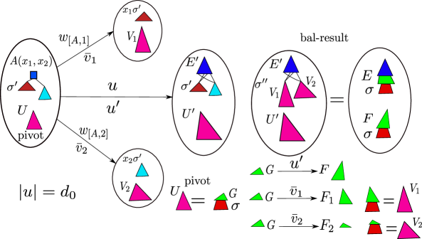
$\overset{A(x_{1},\dots,x_{m})\sigma^{\prime}}{\underset{}{}}\overset{w_{[A,i]}}{\underset{}{\longrightarrow}}\overset{x_{i}\sigma^{\prime}}{\underset{}{}}$ (or $w_{[A,i]}$ does not exist)

$\rho\,=\,\overset{A(x_{1},\dots,x_{m})\sigma^{\prime}}{\underset{U}{}}\hskip 8.00003pt\overset{u}{\underset{u^{\prime}}{\longrightarrow}}\hskip 8.00003pt\overset{E^{\prime}\sigma^{\prime}}{\underset{U^{\prime}}{}}$           $\rho^{\prime}\,=\,\overset{A(x_{1},\dots,x_{m})\sigma^{\prime}}{\underset{U}{}}\overset{u}{\underset{u^{\prime}}{\longrightarrow}}\overset{E^{\prime}\sigma^{\prime}}{\underset{U^{\prime}}{}}\odot\overset{E^{\prime}\sigma^{\prime\prime}}{\underset{U^{\prime}}{}}$     where $x_{i}\sigma^{\prime\prime}=V_{i}$

$\overset{U}{\underset{}{}}\overset{\bar{v}_{i}}{\underset{}{\longrightarrow}}\overset{V_{i}}{\underset{}{}}$ ($V_{i}=U$ when $w_{[A,i]}$ does not exist)

Figure 6: Balancing step $\rho\vdash_{L}\rho^{\prime}$ ($|u|=d_{0}$, $i$ ranges over $[1,m]$, $\textsc{el}(x_{i}\sigma^{\prime},V_{i})>\textsc{el}(E^{\prime}\sigma^{\prime},U^{\prime})$)

Balancing steps, their pivots and balanced results.

Informally speaking, a play $\overset{T}{\underset{U}{}}\overset{u}{\underset{u^{\prime}}{\longrightarrow}}\overset{T^{\prime}}{\underset{U^{\prime}}{}}$ enables left balancing if $T\xrightarrow{u}T^{\prime}$ misses the opportunity to sink to a root-successor as quickly as possible (recall $w_{[A,i]}$ and $d_{0}$ defined around (6)). A left balancing is illustrated in Figure 6 (in both a pictorial and a textual form). We start with a simple example, and only then we give a formal definition.

Let us consider a play of the form

$\overset{T=A(G_{1},G_{2})}{\underset{U}{}}\overset{r_{1}}{\underset{r_{1}^{\prime}}{\longrightarrow}}\overset{B(C(G_{2},G_{1}),G_{1})}{\underset{U_{1}}{}}\overset{r_{2}}{\underset{r_{2}^{\prime}}{\longrightarrow}}\overset{B^{\prime}(G_{1},C(G_{2},G_{1}))=T^{\prime}}{\underset{U^{\prime}}{}}$

where $r_{1}$ is $A(x_{1},x_{2})\xrightarrow{a_{1}}B(C(x_{2},x_{1}),x_{1})$, and $r_{2}$ is $B(x_{1},x_{2})\xrightarrow{a_{2}}B^{\prime}(x_{2},x_{1})$. Let $r_{3}$ be $A(x_{1},x_{2})\xrightarrow{a_{3}}x_{1}$, hence we also have $A(G_{1},G_{2})\xrightarrow{a_{3}}G_{1}$. (Therefore the path $T\xrightarrow{r_{1}r_{2}}T^{\prime}$ clearly missed the opportunity to sink to $G_{1}$ as quickly as possible.) Since $T\xrightarrow{a_{3}}G_{1}$, there must be a transition $U\xrightarrow{a_{3}}V_{1}$, generated by a rule $r^{\prime}_{3}$, such that $\textsc{el}(G_{1},V_{1})\geq\textsc{el}(T,U)-1$ (by Proposition 1(3)); hence $\textsc{el}(G_{1},V_{1})>\textsc{el}(T^{\prime},U^{\prime})$ (since $\textsc{el}(T^{\prime},U^{\prime})=\textsc{el}(T,U)-2$ by the definition of plays). In $T^{\prime}=B^{\prime}(G_{1},C(G_{2},G_{1}))$ we can thus replace $G_{1}$ with $V_{1}$ without affecting $\textsc{el}(T^{\prime},U^{\prime})$; indeed, we have $\textsc{el}(T^{\prime},B^{\prime}(V_{1},C(G_{2},V_{1}))\geq\textsc{el}(G_{1},V_{1})$ (using Proposition 3(2)), and $\textsc{el}(G_{1},V_{1})>\textsc{el}(T^{\prime},U^{\prime})$ thus entails that $\textsc{el}(B^{\prime}(V_{1},C(G_{2},V_{1})),U^{\prime})=\textsc{el}(T^{\prime},U^{\prime})$ (by Proposition 1(1)). If also $G_{2}$ can be reached from $A(G_{1},G_{2})$ in less than two steps, we similarly get $V_{2}$, where $U\xrightarrow{r^{\prime}_{4}}V_{2}$ for some $r^{\prime}_{4}$, so that $\textsc{el}(B^{\prime}(V_{1},C(V_{2},V_{1})),U^{\prime})=\textsc{el}(T^{\prime},U^{\prime})$; hence

$\overset{A(G_{1},G_{2})}{\underset{U}{}}\overset{r_{1}r_{2}}{\underset{r_{1}^{\prime}r^{\prime}_{2}}{\longrightarrow}}\overset{T^{\prime}}{\underset{U^{\prime}}{}}\odot\overset{B^{\prime}(V_{1},C(V_{2},V_{1}))}{\underset{U^{\prime}}{}}$

is a well-defined modified play in this case. Here $U$ is the “pivot”, and we note that $U^{\prime},V_{1},V_{2}$ are all reachable from $U$ in at most two steps. Hence if we present $U$ in a “$2$-top form”, say $U=G\sigma$ where $G=A_{0}(A_{1}(x_{1},x_{2}),A_{2}(x_{3},x_{4}))$, then we have $U^{\prime}=F\sigma$, $V_{1}=F_{1}\sigma$, $V_{2}=F_{2}\sigma$ where $G\xrightarrow{r^{\prime}_{1}r^{\prime}_{2}}F$, $G\xrightarrow{r^{\prime}_{3}}F_{1}$, $G\xrightarrow{r^{\prime}_{4}}F_{2}$. Now the “bal-result” $(T^{\prime\prime},U^{\prime})=(B^{\prime}(V_{1},C(V_{2},V_{1})),U^{\prime})$ can be presented as $(E\sigma,F\sigma)$ where $E=B^{\prime}(F_{1},C(F_{2},F_{1}))$; we note that in $U=G\sigma$ the top $G$ is small, hence also $E,F$ are small, while the terms $x\sigma$ might be large. We now formalize (and generalize) the observation that has been exemplified.

We again consider a fixed general grammar $\mathcal{G}=(\mathcal{N},\Sigma,\mathcal{R})$, and the numbers $m$ (7) and $d_{0}$ (6). We say that a play $\rho=\overset{T}{\underset{U}{}}\overset{u}{\underset{u^{\prime}}{\longrightarrow}}\overset{T^{\prime}}{\underset{U^{\prime}}{}}$ enables $L$-balancing if $|u|=d_{0}$ (hence also $|u^{\prime}|=d_{0}$) and $T\xrightarrow{u}T^{\prime}$ is root-performable, i.e., $T=A(x_{1},\dots,x_{m})\sigma^{\prime}$, $A(x_{1},\dots,x_{m})\xrightarrow{u}E^{\prime}$, and thus $T^{\prime}=E^{\prime}\sigma^{\prime}$ (where $A\in\mathcal{N}$, $E^{\prime}\in\textsc{Terms}_{\mathcal{N}}$, $\textsc{var}(E^{\prime})\subseteq\{x_{1},\dots,x_{m}\}$). We can thus write

$\rho\,=\,\overset{T}{\underset{U}{}}\overset{u}{\underset{u^{\prime}}{\longrightarrow}}\overset{T^{\prime}}{\underset{U^{\prime}}{}}\,=\,\overset{A(x_{1},\dots,x_{m})\sigma^{\prime}}{\underset{U}{}}\overset{u}{\underset{u^{\prime}}{\longrightarrow}}\overset{E^{\prime}\sigma^{\prime}}{\underset{U^{\prime}}{}}$ .

(We have not excluded that $E^{\prime}=x_{i}$ for some $i\in[1,m]$.)

In the described case, in $T^{\prime}$ we can replace each occurrence of a root-successor of $T$ (which is $x_{i}\sigma^{\prime}$ for $i\in[1,m]$) with a term that is shortly reachable from $U$ so that $\textsc{el}(T^{\prime},U^{\prime})$ is unaffected by this replacement; we now make this claim more precise, referring again to the illustration in Figure 6.

Suppose $A(x_{1},\dots,x_{m})\xrightarrow{w_{[A,i]}}x_{i}$ (cf. the definitions around (6)), hence $T\xrightarrow{w_{[A,i]}}x_{i}\sigma^{\prime}$; since $\textsc{el}(T,U)=d_{0}+\textsc{el}(T^{\prime},U^{\prime})\geq d_{0}$ and $|w_{[A,i]}|<d_{0}$, there must be $\bar{v}_{i}\in\mathcal{R}^{+}$ and a term $V_{i}$ such that $|\bar{v}_{i}|=|w_{[A,i]}|$, $\textsc{lab}(\bar{v}_{i})=\textsc{lab}(w_{[A,i]})$, $U\xrightarrow{\bar{v}_{i}}V_{i}$, and $\textsc{el}(x_{i}\sigma^{\prime},V_{i})\geq\textsc{el}(T,U)-|w_{[A,i]}|>\textsc{el}(T,U)-d_{0}=\textsc{el}(T^{\prime},U^{\prime})$ (we use Proposition 1(3)). We can thus reason for all $i\in[1,m]$. If there is no $w_{[A,i]}$ for some $i\in[1,m]$, then $x_{i}\sigma^{\prime}$ is not “exposable” in $T=A(x_{1},\dots,x_{m})\sigma^{\prime}$, hence not in $T^{\prime}=E^{\prime}\sigma^{\prime}$ either, and $x_{i}\sigma^{\prime}$ can be replaced by any term without changing the equivalence class of $T^{\prime}$; in this case we put $V_{i}=U$, thus having $U\xrightarrow{\varepsilon}V_{i}$. Therefore $\textsc{el}(E^{\prime}\sigma^{\prime},U^{\prime})=\textsc{el}(E^{\prime}\sigma^{\prime\prime},U^{\prime})$ where $x_{i}\sigma^{\prime\prime}=V_{i}$ for all $i\in[1,m]$ (by using Propositions 3(2) and 1(1)).

Hence for a play $\rho=\overset{T}{\underset{U}{}}\overset{u}{\underset{u^{\prime}}{\longrightarrow}}\overset{T^{\prime}}{\underset{U^{\prime}}{}}$ in the above notation we can soundly define an $L$-balancing step $\rho\vdash_{L}\rho^{\prime}$ where $\rho^{\prime}$ is a modified play $\rho^{\prime}=\rho\odot(E^{\prime}\sigma^{\prime\prime},U^{\prime})$, depicted in Fig.6. For such an $L$-balancing step $\rho\vdash_{L}\rho^{\prime}$, the term $U$ is called the pivot and the pair $(E^{\prime}\sigma^{\prime\prime},U^{\prime})$ is called the bal-result.

An $R$-balancing step $\rho\vdash_{R}\rho^{\prime}$ is defined symmetrically: if in $\rho=\overset{T}{\underset{U}{}}\overset{u}{\underset{u^{\prime}}{\longrightarrow}}\overset{T^{\prime}}{\underset{U^{\prime}}{}}$ we have $|u|=|u^{\prime}|=d_{0}$ and $U\xrightarrow{u^{\prime}}U^{\prime}$ is root-performable, and presented as $A(x_{1},\dots,x_{m})\sigma^{\prime}\xrightarrow{u^{\prime}}F^{\prime}\sigma^{\prime}$, then we can soundly define

$\overset{T}{\underset{A(x_{1},\dots,x_{m})\sigma^{\prime}}{}}\overset{u}{\underset{u^{\prime}}{\longrightarrow}}\overset{T^{\prime}}{\underset{F^{\prime}\sigma^{\prime}}{}}\,\vdash_{R}\,\overset{T}{\underset{A(x_{1},\dots,x_{m})\sigma^{\prime}}{}}\overset{u}{\underset{u^{\prime}}{\longrightarrow}}\overset{T^{\prime}}{\underset{F^{\prime}\sigma^{\prime}}{}}\odot\overset{T^{\prime}}{\underset{F^{\prime}\sigma^{\prime\prime}}{}}$ ;

here $T$ is the pivot and $(T^{\prime},F^{\prime}\sigma^{\prime\prime})$ is the bal-result.

Relation of the tops of the pivot and of the bal-result.

We now look in more detail at the fact that the pivot of a balancing step and the respective bal-result can be written $G\sigma$ and $(E\sigma,F\sigma)$ for specifically related small “tops” $G,E,F$ (as is also depicted in Figure 6).

We say that a finite term $G$ is a $p$-top, for $p\in\mathbb{N}_{+}$, if $0pt(G)\leq p$, each depth-$p$ subterm is a variable, and $\textsc{var}(G)=\{x_{1},\dots,x_{n}\}$ for some $n\in\mathbb{N}$; hence $n\leq m^{p}$ (for $m$ being the maximum arity of nonterminals (7)).

We note that each term $W$ has a $p$-top form $G\sigma$, i.e., $W=G\sigma$, $G$ is a $p$-top, $\textsc{supp}(\sigma)\subseteq\textsc{var}(G)$, and we have $x\sigma\in\textsc{Var}$ for each $x$ occurring in $G$ in depth less than $p$. (Only a branch of $W$ that finishes with a variable in depth less than $p$ gives rise to such a branch in $G$.) E.g., a $2$-top form of $A(B(x_{9},C(x_{3},x_{6})),x_{9})$ is $G\sigma$ where $G=A(B(x_{1},x_{2}),x_{3})$ and $\sigma=[x_{1}/x_{9},x_{2}/C(x_{3},x_{6}),x_{3}/x_{9}]$; another $2$-top form of this term is $G^{\prime}\sigma^{\prime}$ where $G^{\prime}=A(B(x_{1},x_{2}),x_{1})$ and $\sigma^{\prime}=[x_{1}/x_{9},x_{2}/C(x_{3},x_{6})]$. (We could strengthen the definition to get the unique $p$-top form to each term, but this is not necessary.)

We say that $G\sigma$ is a $p$-safe form of $W$ if $W=G\sigma$ and $W\xrightarrow{v}$, $|v|\leq p$, implies $G\xrightarrow{v}$ (i.e., each word $v\in\mathcal{R}^{*}$ of length at most $p$ that is performable from $W$ is also performable from $G$). We easily observe that each $p$-top form $G\sigma$ of $W$ is also a $p$-safe form of $W$.

The next proposition follows immediately from the definition of balancing steps.

Proposition 12.

Let $W$ be the pivot and $(T^{\prime\prime},U^{\prime\prime})$ the bal-result of an $L$-balancing step. Then for any $d_{0}$-safe form $G\sigma$ of $W$ we have $(T^{\prime\prime},U^{\prime\prime})=(E\sigma,F\sigma)$ where

• $G\xrightarrow{u^{\prime}}F$ for some $u^{\prime}\in\mathcal{R}^{+}$, $|u^{\prime}|=d_{0}$;

• $E=E^{\prime}\overline{\sigma}$ where $A(x_{1},\dots,x_{m})\xrightarrow{u}E^{\prime}$ for some $A\in\mathcal{N}$, $u\in\mathcal{R}^{+}$, $|u|=d_{0}$, and for all $i\in[1,m]$ we have $G\xrightarrow{\overline{v}_{i}}F_{i}$ where $F_{i}=x_{i}\overline{\sigma}$, for some $\overline{v}_{i}$, $|\overline{v}_{i}|<d_{0}$ (hence $T^{\prime\prime}=E\sigma=E^{\prime}\overline{\sigma}\sigma=E^{\prime}\sigma^{\prime\prime}$ where $W\xrightarrow{\overline{v}_{i}}x_{i}\sigma^{\prime\prime}$, for all $i\in[1,m]$).

A symmetric claim holds if $W$, $(T^{\prime\prime},U^{\prime\prime})$ correspond to an $R$-balancing step.

We note a concrete consequence for future use. (Fig. 2 might be again helpful.)

Corollary 13.

Let $G\sigma$ be a $d_{0}$-safe form of $W$. If $W$ is the pivot of a balancing step, then the respective bal-result can be written as $(E\sigma,F\sigma)$ where $\textsc{var}(E,F)\subseteq\textsc{var}(G)$ and

$\textsc{Size}(E,F)\leq\textsc{Size}(G)+(m{+}2)\cdot d_{0}\cdot\textsc{SInc}$.

Proof.

W.l.o.g. we assume an $L$-balancing step, and use $E=E^{\prime}\overline{\sigma}$ and $F$ guaranteed by Proposition 12, where $x_{i}\overline{\sigma}=F_{i}$ for all $i\in[1,m]$. We thus have

$$\textsc{Size}(E,F)\leq\textsc{NtSize}(E^{\prime})+\textsc{Size}(\{F,F_{1},F_{2},\dots,F_{m}\}),$$

since for presenting $E$ we redirect each arc in $E^{\prime}$ that leads to $x_{i}$ towards the root of $F_{i}$ (for $i\in[1,m]$). Since $A(x_{1},\dots,x_{m})\xrightarrow{u}E^{\prime}$ where $|u|=d_{0}$, we have $\textsc{NtSize}(E^{\prime})\leq d_{0}\cdot\textsc{SInc}$. Since all $F,F_{1},F_{2},\dots,F_{m}$ are reachable from $G$ in at most $d_{0}$ steps, we get $\textsc{Size}(\{F,F_{1},F_{2},\dots,F_{m}\})\leq\textsc{Size}(G)+(m+1)\cdot d_{0}\cdot\textsc{SInc}$ by Proposition 5(3); moreover, all sets $\textsc{var}(F)$ and $\textsc{var}(F_{i})$, $i\in[1,m]$, are thus subsets of $\textsc{var}(G)$. The claim follows. ∎

We derive a small bound on the number of bal-results when the pivot is fixed. We put

$$d_{1}=2\cdot|\mathcal{N}|\cdot(\max\{d_{0},|\mathcal{R}|^{d_{0}}\})^{m+2}$$ (16)

(referring to the grammar $\mathcal{G}=(\mathcal{N},\Sigma,\mathcal{R})$).

Proposition 14.

The number of bal-results related to a fixed pivot $W$ is at most $d_{1}$.

Proof.

Given $W$, we fix its $d_{0}$-safe form $G\sigma$ (e.g., a $d_{0}$-top form). Now we suppose that $W=G\sigma$ is the pivot of an $L$-balancing step; let $(E\sigma,F\sigma)=(E^{\prime}\overline{\sigma}\sigma,F\sigma)$ be the respective bal-result, as captured by Proposition 12. We have at most $|\mathcal{R}|^{d_{0}}$ options for $u^{\prime}$ determining $F$, and at most $|\mathcal{N}|\cdot|\mathcal{R}|^{d_{0}}$ options for $E^{\prime}$. For each $i\in[1,m]$, we have at most $1+|\mathcal{R}|^{1}+|\mathcal{R}|^{2}\cdots+|\mathcal{R}|^{d_{0}-1}\leq\max\{d_{0},|\mathcal{R}|^{d_{0}}\}$ options for $F_{i}$. Altogether we get no more than $|\mathcal{N}|\cdot(\max\{d_{0},|\mathcal{R}|^{d_{0}}\})^{m+2}$ options for the bal-result. The same number bounds the possible bal-results of $R$-balancing steps with the pivot $W$, hence the claim follows. ∎

Balanced modified plays, and pivot paths.

We now describe a balancing policy, yielding a sequence of balancing steps that transform a completed play to a “balanced” modified play; the idea of this policy (in a different framework) can be traced back to Sénizergues [1] (and was also used by Stirling [14]).

Let $T_{0}\not\sim U_{0}$ and let $\pi$ be a completed play $\pi$ from $(T_{0},U_{0})$. We show a sequence of transformation phases; after $j$ phases we will get a completed modified play from $(T_{0},U_{0})$ of the form

$\pi_{j}=\mu_{0}\rho^{\prime}_{1}\mu_{1}\rho^{\prime}_{2}\cdots\mu_{j-1}\rho^{\prime}_{j}\pi^{\prime}_{j}$

where $\pi^{\prime}_{j}$ is a play to be transformed in the $(j{+}1)$-th phase. We start with $\pi_{0}=\pi^{\prime}_{0}=\pi$. In general $\pi^{\prime}_{j}$ is not a suffix of $\pi$ but the lengths of the modified plays $\pi_{0},\pi_{1},\pi_{2},\dots$ are the same (recall Proposition 11). In the end we get a balanced modified play $\pi_{\ell}=\mu_{0}\rho^{\prime}_{1}\mu_{1}\rho^{\prime}_{2}\cdots\mu_{\ell-1}\rho^{\prime}_{\ell}\pi^{\prime}_{\ell}$ (for some $\ell\geq 0$) where $\pi^{\prime}_{\ell}$ is non-transformable; this final modified play $\pi_{\ell}=\mu_{0}\rho^{\prime}_{1}\mu_{1}\rho^{\prime}_{2}\cdots\mu_{\ell-1}\rho^{\prime}_{\ell}\mu_{\ell}$ (where $\mu_{\ell}=\pi^{\prime}_{\ell}$) can be also presented as

$$\left[\overset{T_{0}}{\underset{U_{0}}{}}\overset{v_{0}}{\underset{v^{\prime}_{0}}{\longrightarrow}}\overset{T_{1}}{\underset{U_{1}}{}}\right]\left[\overset{T_{1}}{\underset{U_{1}}{}}\overset{u_{1}}{\underset{u^{\prime}_{1}}{\longrightarrow}}\overset{T^{\prime}_{1}}{\underset{U^{\prime}_{1}}{}}\odot\overset{T^{\prime\prime}_{1}}{\underset{U^{\prime\prime}_{1}}{}}\right]\left[\overset{T^{\prime\prime}_{1}}{\underset{U^{\prime\prime}_{1}}{}}\overset{v_{1}}{\underset{v^{\prime}_{1}}{\longrightarrow}}\overset{T_{2}}{\underset{U_{2}}{}}\right]\left[\overset{T_{2}}{\underset{U_{2}}{}}\overset{u_{2}}{\underset{u^{\prime}_{2}}{\longrightarrow}}\overset{T^{\prime}_{2}}{\underset{U^{\prime}_{2}}{}}\odot\overset{T^{\prime\prime}_{2}}{\underset{U^{\prime\prime}_{2}}{}}\right]\cdots\left[\overset{T_{\ell}}{\underset{U_{\ell}}{}}\overset{u_{\ell}}{\underset{u^{\prime}_{\ell}}{\longrightarrow}}\overset{T^{\prime}_{\ell}}{\underset{U^{\prime}_{\ell}}{}}\odot\overset{T^{\prime\prime}_{\ell}}{\underset{U^{\prime\prime}_{\ell}}{}}\right]\left[\overset{T^{\prime\prime}_{\ell}}{\underset{U^{\prime\prime}_{\ell}}{}}\overset{v_{\ell}}{\underset{v^{\prime}_{\ell}}{\longrightarrow}}\overset{T_{\ell+1}}{\underset{U_{\ell+1}}{}}\right]$$

where $\mu_{j}$ is $\overset{T_{0}}{\underset{U_{0}}{}}\overset{v_{0}}{\underset{v^{\prime}_{0}}{\longrightarrow}}\overset{T_{1}}{\underset{U_{1}}{}}$ for $j=0$ and $\overset{T^{\prime\prime}_{j}}{\underset{U^{\prime\prime}_{j}}{}}\overset{v_{j}}{\underset{v^{\prime}_{j}}{\longrightarrow}}\overset{T_{j+1}}{\underset{U_{j+1}}{}}$ for $j\in[1,\ell]$, and $\rho^{\prime}_{j}$ is $\overset{T_{j}}{\underset{U_{j}}{}}\overset{u_{j}}{\underset{u^{\prime}_{j}}{\longrightarrow}}\overset{T^{\prime}_{j}}{\underset{U^{\prime}_{j}}{}}\odot\overset{T^{\prime\prime}_{j}}{\underset{U^{\prime\prime}_{j}}{}}$ (for $j\in[1,\ell]$). By $\rho_{j}$ we denote $\overset{T_{j}}{\underset{U_{j}}{}}\overset{u_{j}}{\underset{u^{\prime}_{j}}{\longrightarrow}}\overset{T^{\prime}_{j}}{\underset{U^{\prime}_{j}}{}}$, and we have either $\rho_{j}\vdash_{L}\rho^{\prime}_{j}$ or $\rho_{j}\vdash_{R}\rho^{\prime}_{j}$. (Hence all $\mu_{j}$ and $\rho_{j}$ are plays, while $\rho^{\prime}_{j}$ is a modified play resulting from $\rho_{j}$ by a balancing step.) By our conventions (and associativity of $\odot$) we can present $\pi_{\ell}=\mu_{0}\rho^{\prime}_{1}\mu_{1}\rho^{\prime}_{2}\cdots\mu_{\ell-1}\rho^{\prime}_{\ell}\mu_{\ell}$ also as

$$\left[\overset{T_{0}}{\underset{U_{0}}{}}\overset{v_{0}}{\underset{v^{\prime}_{0}}{\longrightarrow}}\overset{T_{1}}{\underset{U_{1}}{}}\overset{u_{1}}{\underset{u^{\prime}_{1}}{\longrightarrow}}\overset{T^{\prime}_{1}}{\underset{U^{\prime}_{1}}{}}\right]\odot\left[\overset{T^{\prime\prime}_{1}}{\underset{U^{\prime\prime}_{1}}{}}\overset{v_{1}}{\underset{v^{\prime}_{1}}{\longrightarrow}}\overset{T_{2}}{\underset{U_{2}}{}}\overset{u_{2}}{\underset{u^{\prime}_{2}}{\longrightarrow}}\overset{T^{\prime}_{2}}{\underset{U^{\prime}_{2}}{}}\right]\odot\left[\overset{T^{\prime\prime}_{2}}{\underset{U^{\prime\prime}_{2}}{}}\overset{v_{2}}{\underset{v^{\prime}_{2}}{\longrightarrow}}\cdots\cdots\overset{T_{\ell}}{\underset{U_{\ell}}{}}\overset{u_{\ell}}{\underset{u^{\prime}_{\ell}}{\longrightarrow}}\overset{T^{\prime}_{\ell}}{\underset{U^{\prime}_{\ell}}{}}\right]\odot\left[\overset{T^{\prime\prime}_{\ell}}{\underset{U^{\prime\prime}_{\ell}}{}}\overset{v_{\ell}}{\underset{v^{\prime}_{\ell}}{\longrightarrow}}\overset{T_{\ell+1}}{\underset{U_{\ell+1}}{}}\right]$$. (17)

There are $\ell$ (occurrences of) pivots $W_{1},W_{2},\cdots,W_{\ell}$ in (17), where $W_{j}\in\{T_{j},U_{j}\}$ for each $j\in[1,\ell]$; the bal-result corresponding to $W_{j}$ is $(T^{\prime\prime}_{j},U^{\prime\prime}_{j})$. Though the pivots $W_{j}$ can be changing their sides (we can have, e.g., $W_{j}=U_{j}$ and $W_{j+1}=T_{j+1}$), they will be on one specific pivot path in the LTS $\mathcal{L}^{\textsc{r}}_{\mathcal{G}}$, denoted

$$W_{0}\xrightarrow{w_{0}}W_{1}\xrightarrow{w_{1}}W_{2}\cdots\xrightarrow{w_{\ell-1}}W_{\ell}\xrightarrow{w_{\ell}}W_{\ell+1}$$ (18)

and defined below; we will have $W_{0}\in\{T_{0},U_{0}\}$ and $W_{\ell+1}\in\{T_{\ell+1},U_{\ell+1}\}$ but $W_{0},W_{\ell+1}$ are no pivots, except the case $w_{0}=\varepsilon$ and $W_{0}=W_{1}$. The pivot path will be a useful ingredient for applying our bound on $(n,s,g)$-sequences (Lemma 10).

Now we describe the transformation phases (as non-effective procedures), giving also a finer presentation of $\mu_{j}$ ($j\in[1,\ell]$) as $\mu_{j}=\mu^{\textsc{u}}_{j}$ or $\mu_{j}=\mu^{\textsc{u}}_{j}\mu^{\textsc{s}}_{j}$ (u for “unclear”, s for “sinking”) to be discussed later. The first phase, starting with $\pi_{0}=\pi$, works as follows:

1. If possible, present $\pi_{0}$ as $\mu_{0}\rho_{1}\pi^{\prime}$ where $\rho_{1}$ enables a balancing step (on any side) and $\mu_{0}\rho_{1}$ is the shortest possible. If there is no such presentation of $\pi_{0}$, then put $\mu_{0}=\pi_{0}$ and halt (here $\ell=0$). In this case we do not need to define the path (18).

2. Replace $\rho_{1}$ with $\rho^{\prime}_{1}$ where $\rho_{1}\vdash_{L}\rho^{\prime}_{1}$ or $\rho_{1}\vdash_{R}\rho^{\prime}_{1}$ (choosing arbitrarily when $\rho_{1}$ allows both $L$-balancing and $R$-balancing). Finally replace $\pi^{\prime}$ with a completed play $\pi^{\prime}_{1}$ from the bal-result, i.e., from $\textsc{End}(\rho^{\prime}_{1})$, thus getting $\pi_{1}=\mu_{0}\rho^{\prime}_{1}\pi^{\prime}_{1}$ where $\mu_{0}\rho^{\prime}_{1}=\overset{T_{0}}{\underset{U_{0}}{}}\overset{v_{0}}{\underset{v^{\prime}_{0}}{\longrightarrow}}\overset{T_{1}}{\underset{U_{1}}{}}\overset{u_{1}}{\underset{u^{\prime}_{1}}{\longrightarrow}}\overset{T^{\prime}_{1}}{\underset{U^{\prime}_{1}}{}}\odot\overset{T^{\prime\prime}_{1}}{\underset{U^{\prime\prime}_{1}}{}}$. We also define the prefix $W_{0}\xrightarrow{w_{0}}W_{1}$ of (18): if we have $\rho_{1}\vdash_{L}\rho^{\prime}_{1}$, hence $W_{1}=U_{1}$, then this prefix is $U_{0}\xrightarrow{v^{\prime}_{0}}U_{1}$; if $\rho_{1}\vdash_{R}\rho^{\prime}_{1}$, hence $W_{1}=T_{1}$, then the prefix is $T_{0}\xrightarrow{v_{0}}T_{1}$.

For $j\geq 1$, the $(j{+}1)$-th phase starts with $\pi_{j}=\mu_{0}\rho^{\prime}_{1}\mu_{1}\rho^{\prime}_{2}\cdots\mu_{j-1}\rho^{\prime}_{j}\pi^{\prime}_{j}$ where the last balancing step was either left, $\rho_{j}\vdash_{L}\rho^{\prime}_{j}$, or right, $\rho_{j}\vdash_{R}\rho^{\prime}_{j}$. We describe the $(j{+}1)$-th phase for the case $\rho_{j}\vdash_{L}\rho^{\prime}_{j}$; the other case is symmetric. We recall Figure 6 and present $\rho^{\prime}_{j}\pi^{\prime}_{j}$ as

$\overset{A(x_{1},\dots,x_{m})\sigma^{\prime}}{\underset{U_{j}}{}}\overset{u_{j}}{\underset{u^{\prime}_{j}}{\longrightarrow}}\overset{E^{\prime}\sigma^{\prime}}{\underset{U^{\prime}_{j}}{}}\odot\overset{E^{\prime}\sigma^{\prime\prime}}{\underset{U^{\prime}_{j}}{}}\overset{v}{\underset{v^{\prime}}{\longrightarrow}}$ .

We have also already defined the prefix $W_{0}\xrightarrow{w_{0}}W_{1}\xrightarrow{w_{1}}W_{2}\cdots\xrightarrow{w_{j-1}}W_{j}$ of (18), and we have $W_{j}=U_{j}$ in our considered case $\rho_{j}\vdash_{L}\rho^{\prime}_{j}$.

Informally, the $(j{+}1)$-phase aims to make a balancing step in $\pi^{\prime}_{j}$ as early as possible but balancing at the opposite side than previously is a bit constrained. In our case a future right balancing would entail that the next pivot is on the path $E^{\prime}\sigma^{\prime\prime}\xrightarrow{v}$, and we first have to wait until a term $x_{i}\sigma^{\prime\prime}$ is exposed (i.e., until a prefix of $v$ exposes one of $V_{1},V_{2}$ in Figure 6, where $U$ represents the last pivot $U_{j}$). Only then a right balancing is allowed. This exposing must obviously happen soon (i.e., for a short prefix of $v$) if a further left balancing is not enabled for a while (since in this case $E^{\prime}\sigma^{\prime\prime}\xrightarrow{v}$ must be quickly sinking along a branch of $E^{\prime}$). Hence if even under this constraint the earliest next balancing will be a right balancing, then the next pivot $T_{j+1}$ will be the final term on a path $E^{\prime}\sigma^{\prime\prime}\xrightarrow{v_{j1}}x_{i}\sigma^{\prime\prime}\xrightarrow{v_{j2}}T_{j+1}$ where $v_{j1}v_{j2}$ is a prefix of $v$ and $v_{j_{1}}$ is short. Since $x_{i}\sigma^{\prime\prime}$ is reachable by a short $\bar{v}$ from the last pivot $U_{j}$ (e.g., if $x_{i}\sigma^{\prime\prime}=V_{2}$ in Figure 6, then we use $U\xrightarrow{\bar{v}_{2}}V_{2}$), we continue building the pivot path smoothly: in our case $W_{j}\xrightarrow{w_{j}}W_{j+1}$ will be defined as $U_{j}\xrightarrow{\bar{v}}x_{i}\sigma^{\prime\prime}\xrightarrow{v_{j2}}T_{j+1}$. When a left (unconstrained) balancing is the earliest possibility, $W_{j}\xrightarrow{w_{j}}W_{j+1}$ will be defined simply as $U_{j}\xrightarrow{u^{\prime}_{j}v^{\prime}_{j}}U_{j+1}$ for the respective prefix $v^{\prime}_{j}$ of $v^{\prime}$. (We note that the pivot path gets a bit shorter than the modified play (17) whenever a switch of balancing sides occurrs.) Now we describe the $(j{+}1)$-phase more formally (assuming $\rho_{j}\vdash_{L}\rho^{\prime}_{j}$).

1. If possible, present $\pi^{\prime}_{j}=\overset{E^{\prime}\sigma^{\prime\prime}}{\underset{U^{\prime}_{j}}{}}\overset{v}{\underset{v^{\prime}}{\longrightarrow}}$ as $\mu_{j}\rho_{j+1}\pi^{\prime}$ with the shortest possible $\mu_{j}\rho_{j+1}$ where

   1. either $\rho_{j+1}$ enables $L$-balancing,

   2. or $\rho_{j+1}$ does not enable $L$-balancing but it enables $R$-balancing and the path $E^{\prime}\sigma^{\prime\prime}\xrightarrow{v_{j}}T_{j+1}$ in the play $\mu_{j}=\overset{E^{\prime}\sigma^{\prime\prime}}{\underset{U^{\prime}_{j}}{}}\overset{v_{j}}{\underset{v^{\prime}_{j}}{\longrightarrow}}\overset{T_{j+1}}{\underset{U_{j+1}}{}}$ can be written $E^{\prime}\sigma^{\prime\prime}\xrightarrow{v_{j1}}x_{i}\sigma^{\prime\prime}\xrightarrow{v_{j2}}T_{j+1}$ where $E^{\prime}\xrightarrow{v_{j1}}x_{i}$, for some $i\in[1,m]$. (We recall that $U_{j}\xrightarrow{\overline{v}}x_{i}\sigma^{\prime\prime}$ where $|\overline{v}|<d_{0}$.)

   If there is no such presentation of $\pi^{\prime}_{j}$, then put $\mu_{j}=\pi^{\prime}_{j}$ and halt (here $\ell=j$). In this case we have $\rho^{\prime}_{\ell}\mu_{\ell}=\overset{A(x_{1},\dots,x_{m})\sigma^{\prime}}{\underset{W_{\ell}}{}}\overset{u_{\ell}}{\underset{u^{\prime}_{\ell}}{\longrightarrow}}\overset{E^{\prime}\sigma^{\prime}}{\underset{U^{\prime}_{\ell}}{}}\odot\overset{E^{\prime}\sigma^{\prime\prime}}{\underset{U^{\prime}_{\ell}}{}}\overset{v_{\ell}}{\underset{v^{\prime}_{\ell}}{\longrightarrow}}\overset{T_{\ell+1}}{\underset{U_{\ell+1}}{}}$ and we define $W_{\ell}\xrightarrow{w_{\ell}}W_{\ell+1}$ as $W_{\ell}\xrightarrow{u^{\prime}_{\ell}v^{\prime}_{\ell}}U_{\ell+1}$.

   In each case we get $\mu_{j}=\overset{E^{\prime}\sigma^{\prime\prime}}{\underset{U^{\prime}_{j}}{}}\overset{v_{j}}{\underset{v^{\prime}_{j}}{\longrightarrow}}\overset{T_{j+1}}{\underset{U_{j+1}}{}}$, and if $E^{\prime}\sigma^{\prime\prime}\xrightarrow{v_{j}}T_{j+1}$ can be written $E^{\prime}\sigma^{\prime\prime}\xrightarrow{v_{j1}}x_{i}\sigma^{\prime\prime}\xrightarrow{v_{j2}}T_{j+1}$ where $E^{\prime}\xrightarrow{v_{j1}}x_{i}$ (which holds in the case b) by definition), then we put $\mu_{j}=\mu^{\textsc{u}}_{j}\mu^{\textsc{s}}_{j}$ where $\mu^{\textsc{u}}_{j}=\overset{E^{\prime}\sigma^{\prime\prime}}{\underset{U^{\prime}_{j}}{}}\overset{v_{j1}}{\underset{v^{\prime}_{j1}}{\longrightarrow}}\overset{x_{i}\sigma^{\prime\prime}}{\underset{\overline{U}_{j}}{}}$ and $\mu^{\textsc{s}}_{j}=\overset{x_{i}\sigma^{\prime\prime}}{\underset{\overline{U}_{j}}{}}\overset{v_{j2}}{\underset{v^{\prime}_{j2}}{\longrightarrow}}\overset{T_{j+1}}{\underset{U_{j+1}}{}}$; otherwise $\mu_{j}=\mu^{\textsc{u}}_{j}$.

   (We note that the “unclear” play $\mu^{\textsc{u}}_{j}$ is always short. The “sinking” play $\mu^{\textsc{s}}_{j}$ can be nonempty even if there is no switch in balancing sides, and $\mu^{\textsc{s}}_{j}$ can be long, but both paths in $\mu^{\textsc{s}}_{j}$ are quickly sinking [since no balancing possibility appears].)

2. Replace $\rho_{j+1}$ with $\rho^{\prime}_{j+1}$ where $\rho_{j+1}\vdash_{L}\rho^{\prime}_{j+1}$ in the case a), and $\rho_{j+1}\vdash_{R}\rho^{\prime}_{j+1}$ in the case b). Finally replace $\pi^{\prime}$ with a completed play $\pi^{\prime}_{j+1}$ from the bal-result, i.e., from $\textsc{End}(\rho^{\prime}_{j+1})$, thus getting $\pi_{j+1}=\mu_{0}\rho^{\prime}_{1}\mu_{1}\rho^{\prime}_{2}\cdots\mu_{j}\rho^{\prime}_{j+1}\pi^{\prime}_{j+1}$.

   In the case $\rho_{j+1}\vdash_{L}\rho^{\prime}_{j+1}$ we have $\rho^{\prime}_{j}\mu_{j}=\overset{A(x_{1},\dots,x_{m})\sigma^{\prime}}{\underset{W_{j}}{}}\overset{u_{j}}{\underset{u^{\prime}_{j}}{\longrightarrow}}\overset{E^{\prime}\sigma^{\prime}}{\underset{U^{\prime}_{j}}{}}\odot\overset{E^{\prime}\sigma^{\prime\prime}}{\underset{U^{\prime}_{j}}{}}\overset{v_{j}}{\underset{v^{\prime}_{j}}{\longrightarrow}}\overset{T_{j+1}}{\underset{W_{j+1}}{}}$ and we put $w_{j}=u^{\prime}_{j}v^{\prime}_{j}$, thus defining $W_{j}\xrightarrow{w_{j}}W_{j+1}$.

   In the case $\rho_{j+1}\vdash_{R}\rho^{\prime}_{j+1}$ we have $\rho^{\prime}_{j}\mu_{j}=\overset{A(x_{1},\dots,x_{m})\sigma^{\prime}}{\underset{W_{j}}{}}\overset{u_{j}}{\underset{u^{\prime}_{j}}{\longrightarrow}}\overset{E^{\prime}\sigma^{\prime}}{\underset{U^{\prime}_{j}}{}}\odot\overset{E^{\prime}\sigma^{\prime\prime}}{\underset{U^{\prime}_{j}}{}}\overset{v_{j1}}{\underset{v^{\prime}_{j1}}{\longrightarrow}}\overset{x_{i}\sigma^{\prime\prime}}{\underset{\overline{U}_{j}}{}}\overset{v_{j2}}{\underset{v^{\prime}_{j2}}{\longrightarrow}}\overset{W_{j+1}}{\underset{U_{j+1}}{}}$

   and we define $W_{j}\xrightarrow{w_{j}}W_{j+1}$ by putting $w_{j}=\overline{v}\,v_{j2}$ for a respective $\overline{v}$, $|\overline{v}|<d_{0}$, for which $W_{j}\xrightarrow{\overline{v}}x_{i}\sigma^{\prime\prime}$.

As already mentioned, the work of the $(j{+}1)$-phase in the case $\rho_{j}\vdash_{R}\rho^{\prime}_{j}$ is symmetric; here we have $R$-balancing in the “unconditional” case a), and $L$-balancing in the case b) that now requires a prefix $\mu^{\textsc{u}}_{j}=\overset{T^{\prime}_{j}}{\underset{F^{\prime}\sigma^{\prime\prime}}{}}\overset{v_{j1}}{\underset{v^{\prime}_{j1}}{\longrightarrow}}\overset{\overline{T}_{j}}{\underset{x_{i}\sigma^{\prime\prime}}{}}$ (where $x_{i}\sigma^{\prime\prime}$ is shortly reachable from the last pivot $T_{j}$).

6 Analysis of Balanced Modified Plays

Assuming a given grammar $\mathcal{G}=(\mathcal{N},\Sigma,\mathcal{R})$, we have shown a transformation of a completed play $\pi$ starting in $(T_{0},U_{0})$ (where $T_{0},U_{0}$ can be large regular terms) to a balanced modified play $\pi_{\ell}=\mu_{0}\rho^{\prime}_{1}\mu_{1}\rho^{\prime}_{2}\cdots\mu_{\ell-1}\rho^{\prime}_{\ell}\mu_{\ell}$ in the form (17), repeated here:

$$\left[\overset{T_{0}}{\underset{U_{0}}{}}\overset{v_{0}}{\underset{v^{\prime}_{0}}{\longrightarrow}}\overset{T_{1}}{\underset{U_{1}}{}}\overset{u_{1}}{\underset{u^{\prime}_{1}}{\longrightarrow}}\overset{T^{\prime}_{1}}{\underset{U^{\prime}_{1}}{}}\right]\odot\left[\overset{T^{\prime\prime}_{1}}{\underset{U^{\prime\prime}_{1}}{}}\overset{v_{1}}{\underset{v^{\prime}_{1}}{\longrightarrow}}\overset{T_{2}}{\underset{U_{2}}{}}\overset{u_{2}}{\underset{u^{\prime}_{2}}{\longrightarrow}}\overset{T^{\prime}_{2}}{\underset{U^{\prime}_{2}}{}}\right]\odot\left[\overset{T^{\prime\prime}_{2}}{\underset{U^{\prime\prime}_{2}}{}}\overset{v_{2}}{\underset{v^{\prime}_{2}}{\longrightarrow}}\cdots\cdots\overset{T_{\ell}}{\underset{U_{\ell}}{}}\overset{u_{\ell}}{\underset{u^{\prime}_{\ell}}{\longrightarrow}}\overset{T^{\prime}_{\ell}}{\underset{U^{\prime}_{\ell}}{}}\right]\odot\left[\overset{T^{\prime\prime}_{\ell}}{\underset{U^{\prime\prime}_{\ell}}{}}\overset{v_{\ell}}{\underset{v^{\prime}_{\ell}}{\longrightarrow}}\overset{T_{\ell+1}}{\underset{U_{\ell+1}}{}}\right]$$. (19)

In this section we perform a technical analysis of such $\pi_{\ell}$, to verify that we indeed get specific small numbers $n,s,g$ and $c$ yielding (8), where $\mathcal{E}=\mathcal{E}_{\mathcal{B}}$ for a “sound” $(n,s,g)$-candidate $\mathcal{B}$ (which will turn out equal to the base $\mathcal{B}_{n,s,g}$, as discussed in Section 7). First we recall the discussion at the beginning of Section 5 and give an informal overview of the future analysis.

We recall that in the pivot path

$W_{0}\xrightarrow{w_{0}}W_{1}\xrightarrow{w_{1}}W_{2}\cdots\xrightarrow{w_{\ell-1}}W_{\ell}\xrightarrow{w_{\ell}}W_{\ell+1}$

we have $W_{j}\in\{T_{j},U_{j}\}$ for $j\in[0,\ell{+}1]$, and the pivots $W_{1},W_{2},\dots$, $W_{\ell}$ have the respective related (eqlevel-decreasing) bal-results $(T^{\prime\prime}_{1},U^{\prime\prime}_{1}),(T^{\prime\prime}_{2},U^{\prime\prime}_{2}),\dots,(T^{\prime\prime}_{\ell},U^{\prime\prime}_{\ell})$. Referring to (19), we recall that $u_{i}$ (hence also $u^{\prime}_{i}$) are short since $|u_{i}|=|u^{\prime}_{i}|=d_{0}$ for all $i\in[1,\ell]$ (and $d_{0}$ from (6)). Recalling the discussion around (14), we can present (19) in a refined form as

$$\left[\overset{T_{0}}{\underset{U_{0}}{}}\overset{v_{0}}{\underset{v^{\prime}_{0}}{\longrightarrow}}\overset{T_{1}}{\underset{U_{1}}{}}\overset{u_{1}}{\underset{u^{\prime}_{1}}{\longrightarrow}}\overset{T^{\prime}_{1}}{\underset{U^{\prime}_{1}}{}}\right]\odot\left[\overset{T^{\prime\prime}_{1}}{\underset{U^{\prime\prime}_{1}}{}}\overset{v_{11}}{\underset{v^{\prime}_{11}}{\longrightarrow}}\overset{\overline{T}_{1}}{\underset{\overline{U}_{1}}{}}\overset{v_{12}}{\underset{v^{\prime}_{12}}{\longrightarrow}}\overset{T_{2}}{\underset{U_{2}}{}}\overset{u_{2}}{\underset{u^{\prime}_{2}}{\longrightarrow}}\overset{T^{\prime}_{2}}{\underset{U^{\prime}_{2}}{}}\right]\odot\cdots\odot\left[\overset{T^{\prime\prime}_{\ell}}{\underset{U^{\prime\prime}_{\ell}}{}}\overset{v_{\ell 1}}{\underset{v^{\prime}_{\ell 1}}{\longrightarrow}}\overset{\overline{T}_{\ell}}{\underset{\overline{U}_{\ell}}{}}\overset{v_{\ell 2}}{\underset{v^{\prime}_{\ell 2}}{\longrightarrow}}\overset{T_{\ell+1}}{\underset{U_{\ell+1}}{}}\right]$$; (20)

here $\left[\overset{T^{\prime\prime}_{j}}{\underset{U^{\prime\prime}_{j}}{}}\overset{v_{j}}{\underset{v^{\prime}_{j}}{\longrightarrow}}\overset{T_{j+1}}{\underset{U_{j+1}}{}}\overset{u_{j+1}}{\underset{u^{\prime}_{j+1}}{\longrightarrow}}\overset{T^{\prime}_{j+1}}{\underset{U^{\prime}_{j+1}}{}}\right]$, for $j\in[1,\ell]$, is presented as $\left[\overset{T^{\prime\prime}_{j}}{\underset{U^{\prime\prime}_{j}}{}}\overset{v_{j1}}{\underset{v^{\prime}_{j1}}{\longrightarrow}}\overset{\overline{T}_{j}}{\underset{\overline{U}_{j}}{}}\overset{v_{j2}}{\underset{v^{\prime}_{j2}}{\longrightarrow}}\overset{T_{j+1}}{\underset{U_{j+1}}{}}\overset{u_{j+1}}{\underset{u^{\prime}_{j+1}}{\longrightarrow}}\overset{T^{\prime}_{j+1}}{\underset{U^{\prime}_{j+1}}{}}\right]$ where $v_{j1}$ is short and both paths $\overline{T}_{j}\xrightarrow{v_{j2}}T_{j+1}$ and $\overline{U}_{j}\xrightarrow{v^{\prime}_{j2}}U_{j+1}$ are $d_{0}$-sinking (i.e., in each segment of length $d_{0}$ of these paths a root-successor in the term that starts the segment is exposed); we can have $v_{j2}=\varepsilon$.

The first segment $W_{0}\xrightarrow{w_{1}}W_{1}$ is one of the paths $T_{0}\xrightarrow{v_{0}}T_{1}$ and $U_{0}\xrightarrow{v^{\prime}_{0}}U_{1}$; each of these two paths is $d_{0}$-sinking (since otherwise the first balancing would be possible earlier). For the segment $W_{j}\xrightarrow{w_{j}}W_{j+1}$, $j\in[1,\ell]$, we have four options:

• $U_{j}\xrightarrow{u^{\prime}_{j}v^{\prime}_{j1}}\overline{U}_{j}\xrightarrow{v^{\prime}_{j2}}U_{j+1}$, if $W_{j}=U_{j}$ and $W_{j+1}=U_{j+1}$;

• $T_{j}\xrightarrow{u_{j}v_{j1}}\overline{T}_{j}\xrightarrow{v_{j2}}T_{j+1}$, if $W_{j}=T_{j}$ and $W_{j+1}=T_{j+1}$;

• $U_{j}\xrightarrow{\bar{v}}\overline{T}_{j}\xrightarrow{v_{j_{2}}}T_{j+1}$ for some $\bar{v}$, $|\bar{v}|<d_{0}$, if $W_{j}=U_{j}$ and $W_{j+1}=T_{j+1}$;

• $T_{j}\xrightarrow{\bar{v}}\overline{U}_{j}\xrightarrow{v^{\prime}_{j2}}U_{j+1}$ for some $\bar{v}$, $|\bar{v}|<d_{0}$, if $W_{j}=T_{j}$ and $W_{j+1}=U_{j+1}$.

Hence each $W_{j}\xrightarrow{w_{j}}W_{j+1}$ has a short “unclear” prefix (it is unclear if it sinks or not), followed by a $d_{0}$-sinking suffix (which might be empty, or short, or long …).

This entails that if the path $W_{j}\xrightarrow{w_{j}}W_{j+1}$ visits a subterm of $W_{0}$, which is surely the case for $W_{0}\xrightarrow{w_{0}}W_{1}$, then $W_{j+1}$ is shortly reachable from a subterm of $W_{0}$. Indeed, if $W_{j}\xrightarrow{w_{j}}W_{j+1}$ is $W_{j}\xrightarrow{w^{\prime}_{j}}V\xrightarrow{w^{\prime\prime}_{j}}W_{j+1}$ where $V$ is the last subterm of $W_{0}$ visited by the path $W_{j}\xrightarrow{w_{j}}W_{j+1}$, then $w^{\prime\prime}_{j}$ has a short unclear prefix (maybe empty) followed by a $d_{0}$-sinking suffix; but if this suffix was not short, then it would necessarily expose a root-successor in $V$, which is another subterm of $W_{0}$; this would contradict the choice of $V$. (Figure 2 might be again helpful to realize this fact.)

For each subterm $V$ of $W_{0}$ we certainly have only a small number of terms $W$ that are shortly reachable from $V$. Since there is only a small number of possible bal-results related to each concrete pivot $W$, and the bal-results do not repeat, we get that the number of indices $j\in[0,\ell]$ for which $W_{j}\xrightarrow{w_{j}}W_{j+1}$ visits a subterm of $W_{0}$ is bounded by $d\cdot\textsc{Size}(T_{0},U_{0})$ for a small constant $d$. (We recall that $W_{0}\in\{T_{0},U_{0}\}$.)

We say that a segment of the pivot path of the form

$V\xrightarrow{w}W_{j+1}\xrightarrow{w_{j+1}}W_{j+2}\cdots\xrightarrow{w_{j+z-1}}W_{j+z}\xrightarrow{w^{\prime}}V^{\prime}$

is crucial if $w$ is a nonempty suffix of $w_{j}$, $1\leq z\leq\ell{-}j$, $w^{\prime}$ is a prefix of $w_{j+z}$, $V$ is a subterm of $W_{0}$, and no subterm of $W_{0}$ is visited inside the segment; moreover, either $V^{\prime}$ is a subterm of $W_{0}$ or $V^{\prime}=W_{\ell+1}$ (the end of the pivot path). (We can again look at Figure 2, and imagine that $W_{0}$ is the (maybe large regular) term in the rectangle and $V$ is its subterm determined in the third rectangle, whose root is $B$. The next two steps can be viewed as a prefix of a crucial segment that could finish after many steps later when some of the root-successors of $B$ in the rectangle is exposed and becomes the current root.)

Since each crucial segment is non-sinking (until the last step), it gives rise to an $(n,s,g)$-sequence (for some small $n,s,g$), as was depicted in Figure 5 and discussed in the informal beginning of Section 5. It is thus intuitively clear that the length of any crucial segment of the pivot path, as well as the length of its corresponding segment of the modified play (19), is bounded by $d^{\prime}\cdot\mathcal{E}_{\mathcal{B}_{n,s,g}}$ for a small constant $d^{\prime}$ (and the $(n,s,g)$-base $\mathcal{B}_{n,s,g}$, by Lemma 10).

Since each crucial segment is fully determined by the segment $W_{j}\xrightarrow{w_{j}}W_{j+1}$ in which it starts (and which visits a subterm of $W_{0}$), there are at most $d\cdot\textsc{Size}(T_{0},U_{0})$ crucial segments, and their overall length is thus bounded by $d\cdot\textsc{Size}(T_{0},U_{0})\cdot d^{\prime}\cdot\mathcal{E}_{\mathcal{B}_{n,s,g}}$. Hence we are approaching the required bound

$\textsc{el}(T_{0},U_{0})\leq c\cdot\big{(}\mathcal{E}_{\mathcal{B}_{n,s,g}}\cdot\textsc{Size}(T_{0},U_{0})+(\textsc{Size}(T_{0},U_{0}))^{2}\big{)}$,

for a small constant $c$. The bound $c\cdot(\textsc{Size}(T_{0},U_{0}))^{2}$ serves for bounding the sum of lengths of subpaths of $W_{j}\xrightarrow{w_{j}}W_{j+1}$ (and the corresponding subplays in (19)) when both sides are quickly sinking “inside” the (regular) terms $T_{0}$ and $U_{0}$, respectively. (An extreme case is when there is no balancing since both paths from $T_{0}$ and $U_{0}$, respectively, are $d_{0}$-sinking all the time.) Since the eq-level drops by one in each step of each play in (19), we cannot have a repeat of a pair there. Hence there is some small $c$ such that $c\cdot(\textsc{Size}(T_{0},U_{0}))^{2}$ bounds the number of those pairs in (19) in which both members are “close to” subterms of $T_{0}$ or $U_{0}$. This bounds the sum of lengths of the respective segments of (19) that are sinking “closely to $T_{0},U_{0}$” on both sides.

The claim of Theorem 7 is now almost clear; it will be completed in Section 7 where we show that the respective constant $\mathcal{E}=\mathcal{E}_{\mathcal{B}_{n,s,g}}$ is indeed computable. In the rest of this section we perform a routine (and somewhat tedious) analysis to show some concrete numbers $n,s,g,c$ (cf. Table 1 at the end of the paper).

Refined presentations of balanced modified plays.

Assuming a given grammar $\mathcal{G}=(\mathcal{N},\Sigma,\mathcal{R})$, we fix a completed play $\pi$ from some (maybe large regular terms) $(T_{0},U_{0})$ and its transformation $\pi_{\ell}=\mu_{0}\rho^{\prime}_{1}\mu_{1}\rho^{\prime}_{2}\cdots\mu_{\ell-1}\rho^{\prime}_{\ell}\pi^{\prime}_{\ell}$ in the previous notation; in fact, we also use a finer form and write

$$\pi_{\ell}=\mu^{\textsc{s}}_{0}\rho^{\prime}_{1}\mu^{\textsc{u}}_{1}\mu^{\textsc{s}}_{1}\rho^{\prime}_{2}\mu^{\textsc{u}}_{2}\mu^{\textsc{s}}_{2}\cdots\rho^{\prime}_{\ell}\mu^{\textsc{u}}_{\ell}\mu^{\textsc{s}}_{\ell}$$ (21)

(where the superscript u can be read as “unclear” and s as “sinking”). We add that $\mu^{\textsc{s}}_{0}=\mu_{0}$ and that we view $\varepsilon$ (the empty sequence) also as the empty play, and we put $\mu^{\textsc{s}}_{j}=\varepsilon$ in the cases where $\mu^{\textsc{s}}_{j}$ has not been defined explicitly. As expected, we stipulate $\textsc{length}(\varepsilon)=0$, $\textsc{Pairs}(\varepsilon)=\emptyset$, and $\mu\varepsilon=\varepsilon\mu=\mu$ for all (modified) plays $\mu$.

The presentation (17) is accordingly refined (as in (20)) to

$$\left[\overset{T_{0}}{\underset{U_{0}}{}}\overset{v_{0}}{\underset{v^{\prime}_{0}}{\longrightarrow}}\overset{T_{1}}{\underset{U_{1}}{}}\overset{u_{1}}{\underset{u^{\prime}_{1}}{\longrightarrow}}\overset{T^{\prime}_{1}}{\underset{U^{\prime}_{1}}{}}\right]\odot\left[\overset{T^{\prime\prime}_{1}}{\underset{U^{\prime\prime}_{1}}{}}\overset{v_{11}}{\underset{v^{\prime}_{11}}{\longrightarrow}}\overset{\overline{T}_{1}}{\underset{\overline{U}_{1}}{}}\overset{v_{12}}{\underset{v^{\prime}_{12}}{\longrightarrow}}\overset{T_{2}}{\underset{U_{2}}{}}\overset{u_{2}}{\underset{u^{\prime}_{2}}{\longrightarrow}}\overset{T^{\prime}_{2}}{\underset{U^{\prime}_{2}}{}}\right]\odot\cdots\odot\left[\overset{T^{\prime\prime}_{\ell}}{\underset{U^{\prime\prime}_{\ell}}{}}\overset{v_{\ell 1}}{\underset{v^{\prime}_{\ell 1}}{\longrightarrow}}\overset{\overline{T}_{\ell}}{\underset{\overline{U}_{\ell}}{}}\overset{v_{\ell 2}}{\underset{v^{\prime}_{\ell 2}}{\longrightarrow}}\overset{T_{\ell+1}}{\underset{U_{\ell+1}}{}}\right]$$ (22)

where, for $j\in[1,\ell]$, we have $\mu^{\textsc{u}}_{j}=\overset{T^{\prime\prime}_{j}}{\underset{U^{\prime\prime}_{j}}{}}\overset{v_{j1}}{\underset{v^{\prime}_{j1}}{\longrightarrow}}\overset{\overline{T}_{j}}{\underset{\overline{U}_{j}}{}}$, and either $\mu^{\textsc{s}}_{j}=\overset{\overline{T}_{j}}{\underset{\overline{U}_{j}}{}}\overset{v_{j2}}{\underset{v^{\prime}_{j2}}{\longrightarrow}}\overset{{T}_{j+1}}{\underset{\overline{U}_{j+1}}{}}$ or $\mu^{\textsc{s}}_{j}=\varepsilon$ in which case $v_{j2}=v^{\prime}_{j2}=\varepsilon$, $\overline{T}_{j}=T_{j+1}$, $\overline{U}_{j}=U_{j+1}$.

To explain the use of the superscript s (“sinking”) in $\mu^{\textsc{s}}_{j}$, we introduce a few notions.

An $(A,i)$-sink word $v\in\mathcal{R}^{+}$ (satisfying $A(x_{1},\dots,x_{m})\xrightarrow{v}x_{i}$) is also called a sink-segment; any path of the form $V\xrightarrow{v}V^{\prime}$ is then also understood as a sink-segment (presentable as $A(x_{1},\dots,x_{m})\sigma\xrightarrow{v}x_{i}\sigma$). We say that a path $V\xrightarrow{v}V^{\prime}$ is $d_{0}$-sinking, if $v=v_{1}v_{2}\cdots v_{k+1}$ where $|v_{j}|<d_{0}$ for all $j\in[1,k{+}1]$ and $v_{j}$, $j\in[1,k]$, are sink-segments. A zero-length path $V\xrightarrow{\varepsilon}V$ is $d_{0}$-sinking, by putting $k=0$ and $v_{k+1}=\varepsilon$.

A play $\mu=\overset{T}{\underset{U}{}}\overset{v}{\underset{v^{\prime}}{\longrightarrow}}\overset{T^{\prime}}{\underset{U^{\prime}}{}}$ is $d_{0}$-sinking if both its paths $T\xrightarrow{v}T^{\prime}$ and $U\xrightarrow{v^{\prime}}U^{\prime}$ are $d_{0}$-sinking. In particular, a zero-length play $\mu=\overset{T}{\underset{U}{}}$ is $d_{0}$-sinking, and we also view the empty play $\varepsilon$ as $d_{0}$-sinking.

The above transformation (of $\pi$ to $\pi_{\ell}$) guarantees that all plays $\mu_{0}$, $\mu^{\textsc{s}}_{1}$, $\mu^{\textsc{s}}_{2}$, $\dots$, $\mu^{\textsc{s}}_{\ell}$ are $d_{0}$-sinking (therefore we have put $\mu_{0}=\mu^{\textsc{s}}_{0}$). Indeed, if some $\mu^{\textsc{s}}_{j}$ ($j\in[0,\ell]$) was not $d_{0}$-sinking, then there would be a possibility to make a “legal” balancing step earlier in the respective transformation phase.

The presentations (21) and (22) also yield the corresponding refined version of the pivot path (18):

$$W_{0}\xrightarrow{w^{\textsc{s}}_{0}}W_{1}\xrightarrow{w^{\textsc{u}}_{1}}\overline{W}_{1}\xrightarrow{w^{\textsc{s}}_{1}}W_{2}\xrightarrow{w^{\textsc{u}}_{2}}\overline{W}_{2}\xrightarrow{w^{\textsc{s}}_{2}}\cdots W_{\ell}\xrightarrow{w^{\textsc{u}}_{\ell}}\overline{W}_{\ell}\xrightarrow{w^{\textsc{s}}_{\ell}}W_{\ell+1}$$ (23)

where each segment $\overline{W}_{j}\xrightarrow{w^{\textsc{s}}_{j}}W_{j+1}$ (for $j\in[0,\ell]$ when putting $\overline{W}_{0}=W_{0}$) corresponds to one of the paths in the play $\mu^{\textsc{s}}_{j}$, and is thus $d_{0}$-sinking. More concretely, $W_{0}\xrightarrow{w^{\textsc{s}}_{0}}W_{1}$ (where $w^{\textsc{s}}_{0}=w_{0}$) is either $T_{0}\xrightarrow{v_{0}}T_{1}$ or $U_{0}\xrightarrow{v^{\prime}_{0}}U_{1}$, and $\overline{W}_{j}\xrightarrow{w^{\textsc{s}}_{j}}W_{j+1}$ is either $\overline{T}_{j}\xrightarrow{v_{j2}}T_{j+1}$ or $\overline{U}_{j}\xrightarrow{v^{\prime}_{j2}}U_{j+1}$. Each (“unclear”) segment $W_{j}\xrightarrow{w^{\textsc{u}}_{j}}\overline{W}_{j}$ is one of the following paths:

• $U_{j}\xrightarrow{u^{\prime}_{j}v^{\prime}_{j1}}\overline{U}_{j}$, if $W_{j}=U_{j}$ and $W_{j+1}=U_{j+1}$ (in which case $U^{\prime}_{j}=U^{\prime\prime}_{j}$);

• $T_{j}\xrightarrow{u_{j}v_{j1}}\overline{T}_{j+1}$, if $W_{j}=T_{j}$ and $W_{j+1}=T_{j+1}$ (in which case $T^{\prime}_{j}=T^{\prime\prime}_{j}$);

• $U_{j}\xrightarrow{v}\overline{T}_{j}$ for some $v$, $|v|<d_{0}$, if $W_{j}=U_{j}$ and $W_{j+1}=T_{j+1}$;

• $T_{j}\xrightarrow{v}\overline{U}_{j}$ for some $v$, $|v|<d_{0}$, if $W_{j}=T_{j}$ and $W_{j+1}=U_{j+1}$.

We now note that the length of each segment $\rho^{\prime}_{j}\mu^{\textsc{u}}_{j}=\overset{T_{j}}{\underset{U_{j}}{}}\overset{u_{j}}{\underset{u^{\prime}_{j}}{\longrightarrow}}\overset{T^{\prime}_{j}}{\underset{U^{\prime}_{j}}{}}\odot\overset{T^{\prime\prime}_{j}}{\underset{U^{\prime\prime}_{j}}{}}\overset{v_{j1}}{\underset{v^{\prime}_{j1}}{\longrightarrow}}\overset{\overline{T}_{j}}{\underset{\overline{U}_{j}}{}}$, and of the respective pivot-path segment $W_{j}\xrightarrow{w^{\textsc{u}}_{j}}\overline{W}_{j}$, can be bounded by the small number

$$d_{2}=d_{0}+(1+d_{0}\cdot\textsc{HInc})\cdot(d_{0}-1).$$ (24)

Proposition 15.

For each $j\in[1,\ell]$ we have $|w^{\textsc{u}}_{j}|\leq\textsc{length}(\rho^{\prime}_{j}\mu^{\textsc{u}}_{j})\leq d_{2}$.

Proof.

We have $|w^{\textsc{u}}_{j}|\leq\textsc{length}(\rho^{\prime}_{j}\mu^{\textsc{u}}_{j})$ by the above definitions (since $\textsc{length}(\rho^{\prime}_{j}\mu^{\textsc{u}}_{j})\geq d_{0}$, and either $|w^{\textsc{u}}_{j}|=\textsc{length}(\rho^{\prime}_{j}\mu^{\textsc{u}}_{j})$ or $|w^{\textsc{u}}_{j}|<d_{0}$).

W.l.o.g. we suppose $\rho_{j}\vdash_{L}\rho^{\prime}_{j}$ (illustrated in Fig.6) and present $\rho^{\prime}_{j}\mu^{\textsc{u}}_{j}$ accordingly as

$\rho^{\prime}_{j}\mu^{\textsc{u}}_{j}=\overset{A(x_{1},\dots,x_{m})\sigma^{\prime}}{\underset{U_{j}}{}}\overset{u_{j}}{\underset{u^{\prime}_{j}}{\longrightarrow}}\overset{E^{\prime}\sigma^{\prime}}{\underset{U^{\prime}_{j}}{}}\odot\overset{E^{\prime}\sigma^{\prime\prime}}{\underset{U^{\prime}_{j}}{}}\overset{v_{j1}}{\underset{v^{\prime}_{j1}}{\longrightarrow}}\overset{\overline{T}_{j}}{\underset{\overline{U}_{j}}{}}$

where $A(x_{1},\dots,x_{m})\xrightarrow{u_{j}}E^{\prime}$ and $|u_{j}|=d_{0}$; hence $0pt(E^{\prime})\leq 1+d_{0}\cdot\textsc{HInc}$. We have $\overline{T}_{j}=T_{j+1}$ if $\mu^{\textsc{s}}_{j}=\varepsilon$, and $\overline{T}_{j}=x_{i}\sigma^{\prime\prime}$ (for some $i\in[1,m]$) if $\mu^{\textsc{s}}_{j}\neq\varepsilon$.

The path $E^{\prime}\sigma^{\prime\prime}\xrightarrow{v_{j1}}\overline{T}_{j}$ must be $d_{0}$-sinking (otherwise there would be an earlier next balancing step). Hence $|v_{j1}|\leq 0pt(E^{\prime})\cdot(d_{0}-1)$. We thus get

$\textsc{length}(\rho^{\prime}_{j}\mu^{\textsc{u}}_{j})=|u_{j}|+|v_{j1}|\leq d_{0}+(1+d_{0}\cdot\textsc{HInc})\cdot(d_{0}-1)=d_{2}$.

∎

Having bounded the parts $\rho^{\prime}_{j}\mu^{\textsc{u}}_{j}$, we will now bound the total length of the suffixes of $\mu^{\textsc{s}}_{j}$ that are “close to” $T_{0},U_{0}$; then we will finally bound the number and the length of so-called “crucial segments” of $\pi_{\ell}$ starting with pivots that are also close to $T_{0},U_{0}$ in a sense.

Close sink-parts in $\pi_{\ell}$.

Since $\mu_{0}=\mu^{\textsc{s}}_{0}=\overset{T_{0}}{\underset{U_{0}}{}}\overset{v_{0}}{\underset{v^{\prime}_{0}}{\longrightarrow}}\overset{T_{1}}{\underset{U_{1}}{}}$ is $d_{0}$-sinking, both paths $T_{0}\xrightarrow{v_{0}}T_{1}$ and $U_{0}\xrightarrow{v^{\prime}_{0}}U_{1}$ are frequently visiting subterms of the terms $T_{0}$ and $U_{0}$. Using the fact that no pair repeats along $\pi_{\ell}$ (recall Proposition 11), we now derive a bound on the length of $\mu_{0}$ and other segments that are “close” to $(T_{0},U_{0})$.

For each $j\in[1,\ell]$ where $\mu^{\textsc{s}}_{j}\neq\varepsilon$ we define the presentation $\mu^{\textsc{s}}_{j}=\mu^{\textsc{us}}_{j}\mu^{\textsc{cs}}_{j}$ (the superscript us for “unclear sinking” and cs for “close sinking”) as follows: If some of the paths in the play $\mu^{\textsc{s}}_{j}=\overset{\overline{T}_{j}}{\underset{\overline{U}_{j}}{}}\overset{v_{j2}}{\underset{v^{\prime}_{j2}}{\longrightarrow}}\overset{T_{j+1}}{\underset{U_{j+1}}{}}$ never visits a subterm of $T_{0}$ or $U_{0}$, then $\mu^{\textsc{us}}_{j}=\mu^{\textsc{s}}_{j}$ and $\mu^{\textsc{cs}}_{j}=\varepsilon$. Otherwise we write $\mu^{\textsc{s}}_{j}$ as $\overset{\overline{T}_{j}}{\underset{\overline{U}_{j}}{}}\overset{\overline{v}_{j2}}{\underset{\overline{v}^{\prime}_{j2}}{\longrightarrow}}\overset{\overline{\overline{T}}_{j}}{\underset{\overline{\overline{U}}_{j}}{}}\overset{\overline{\overline{v}}_{j2}}{\underset{\overline{\overline{v}}^{\prime}_{j2}}{\longrightarrow}}\overset{T_{j+1}}{\underset{U_{j+1}}{}}$ for the shortest prefix $\mu^{\textsc{us}}_{j}=\overset{\overline{T}_{j}}{\underset{\overline{U}_{j}}{}}\overset{\overline{v}_{j2}}{\underset{\overline{v}^{\prime}_{j2}}{\longrightarrow}}\overset{\overline{\overline{T}}_{j}}{\underset{\overline{\overline{U}}_{j}}{}}$ such that each of the paths $\overline{T}_{j}\xrightarrow{\overline{v}_{j2}}\overline{\overline{T}}_{j}$ and $\overline{U}_{j}\xrightarrow{\overline{v}^{\prime}_{j2}}\overline{\overline{U}}_{j}$ visits a subterm of $T_{0}$ or $U_{0}$; in this case $\mu^{\textsc{cs}}_{j}=\overset{\overline{\overline{T}}_{j}}{\underset{\overline{\overline{U}}_{j}}{}}\overset{\overline{\overline{v}}_{j2}}{\underset{\overline{\overline{v}}^{\prime}_{j2}}{\longrightarrow}}\overset{T_{j+1}}{\underset{U_{j+1}}{}}$. (Since $\mu^{\textsc{s}}_{j}$ is $d_{0}$-sinking, both paths $\overline{\overline{T}}_{j}\xrightarrow{\overline{\overline{v}}_{j2}}T_{j+1}$ and $\overline{\overline{U}}_{j}\xrightarrow{\overline{\overline{v}}^{\prime}_{j2}}U_{j+1}$ are frequently visiting subterms of the terms $T_{0}$ and $U_{0}$.) If $\mu^{\textsc{s}}_{j}=\varepsilon$, then we put $\mu^{\textsc{us}}_{j}=\mu^{\textsc{cs}}_{j}=\varepsilon$; we also put $\mu_{0}=\mu^{\textsc{s}}_{0}=\mu^{\textsc{cs}}_{0}$ (while $\mu^{\textsc{us}}_{0}=\varepsilon$).

The balanced modified play $\pi_{\ell}$ (21) can be thus presented in more detail as

$$\pi_{\ell}=\mu^{\textsc{cs}}_{0}\rho^{\prime}_{1}\mu^{\textsc{u}}_{1}\mu^{\textsc{us}}_{1}\mu^{\textsc{cs}}_{1}\rho^{\prime}_{2}\mu^{\textsc{u}}_{2}\mu^{\textsc{us}}_{2}\mu^{\textsc{cs}}_{2}\cdots\rho^{\prime}_{\ell}\mu^{\textsc{u}}_{\ell}\mu^{\textsc{us}}_{\ell}\mu^{\textsc{cs}}_{\ell}.$$ (25)

We refer to $\mu^{\textsc{cs}}_{j}$, $j\in[0,\ell]$, as to close sink-parts. The next proposition bounds the total length of close sink-parts in (25), using the small number

$$d_{3}=(\max\{d_{0},|\mathcal{R}|^{d_{0}}\})^{2}$$ (26)

(determined by $\mathcal{G}=(\mathcal{N},\Sigma,\mathcal{R})$).

Proposition 16.

$\sum_{j\in[0,\ell]}\textsc{length}(\mu^{\textsc{cs}}_{j})\leq d_{3}\cdot(\textsc{Size}(T_{0},U_{0}))^{2}$.

Proof.

The number of subterms of $T_{0}$ and $U_{0}$ is $\textsc{Size}(T_{0},U_{0})$, and each term can reach at most $\max\{|\mathcal{R}|^{d_{0}},d_{0}\}$ terms within less than $d_{0}$ steps (since $|\mathcal{R}|^{0}+|\mathcal{R}|^{1}+\cdots+|\mathcal{R}|^{d_{0}-1}\leq|\mathcal{R}|^{d_{0}}$ when $|\mathcal{R}|\geq 2$). Hence there are at most $\big{(}\max\{|\mathcal{R}|^{d_{0}},d_{0}\}\cdot\textsc{Size}(T_{0},U_{0})\,\big{)}^{2}$ elements in $\bigcup_{j\in[0,\ell]}\textsc{Pairs}(\mu^{\textsc{cs}}_{j})$. Since there is no repeat of a pair in $\pi_{\ell}$, the claim follows. ∎

Crucial segments of $\pi_{\ell}$.

For $\pi_{\ell}=\mu^{\textsc{cs}}_{0}\rho^{\prime}_{1}\mu^{\textsc{u}}_{1}\mu^{\textsc{us}}_{1}\mu^{\textsc{cs}}_{1}\rho^{\prime}_{2}\mu^{\textsc{u}}_{2}\mu^{\textsc{us}}_{2}\mu^{\textsc{cs}}_{2}\cdots\rho^{\prime}_{\ell}\mu^{\textsc{u}}_{\ell}\mu^{\textsc{us}}_{\ell}\mu^{\textsc{cs}}_{\ell}$ and the respective pivot path $W_{0}\xrightarrow{w_{0}}W_{1}\xrightarrow{w_{1}}W_{2}\xrightarrow{w_{2}}\cdots W_{\ell}\xrightarrow{w_{\ell}}W_{\ell+1}$, assuming $\ell\geq 1$, we say that $W_{j}$, $j\in[1,\ell]$ is close (which is another variant of closeness to $(T_{0},U_{0})$) if the path $W_{j-1}\xrightarrow{w_{j-1}}W_{j}$ visits a subterm of $T_{0}$ or $U_{0}$; in this case we also write $W_{j-1}\xrightarrow{w_{j-1}}W_{j}$ as

$W_{j-1}\xrightarrow{w^{\prime}_{j-1}}V_{j-1}\xrightarrow{w^{\prime\prime}_{j-1}}W_{j}$

where $V_{j-1}$ is the last subterm of $T_{0}$ or $U_{0}$ in the path (not excluding the cases $V_{j-1}=W_{j-1}$ and $V_{j-1}=W_{j}$). We note that $W_{1}$ is close, since $W_{0}\in\{T_{0},U_{0}\}$.

Let $\{j\in[1,\ell]\mid W_{j}$ is close$\}=\{k_{1},k_{2},\dots,k_{p}\}$ where $1=k_{1}<k_{2}<k_{3}\cdots<k_{p}\leq\ell$; for technical reasons we also put $k_{p+1}=\ell{+}1$. The pivot path can be thus written

$$W_{0}\xrightarrow{w^{\prime}_{0}}[V_{0}\xrightarrow{w^{\prime\prime}_{0}}W_{1}\xrightarrow{w_{1}}\cdots W_{k_{2}-1}]\xrightarrow{w^{\prime}_{k_{2}-1}}\cdots[V_{k_{p}-1}\xrightarrow{w^{\prime\prime}_{k_{p}-1}}W_{k_{p}}\xrightarrow{w_{k_{p}}}\cdots W_{\ell}]\xrightarrow{w_{\ell}}W_{\ell+1}$$ (27)

where the brackets are just highlighting the corresponding segments. We use the segmentation (27) of the pivot path to induce the following segmentation of $\pi_{\ell}$:

$$\mu^{\textsc{cs}}_{0}\big{[}\rho^{\prime}_{1}\cdots\mu^{\textsc{us}}_{k_{2}-1}\big{]}\mu^{\textsc{cs}}_{k_{2}-1}\big{[}\rho^{\prime}_{k_{2}}\cdots\mu^{\textsc{us}}_{k_{3}-1}\big{]}\mu^{\textsc{cs}}_{k_{3}-1}\cdots\cdots\big{[}\rho^{\prime}_{k_{p}}\cdots\mu^{\textsc{us}}_{\ell}\big{]}\mu^{\textsc{cs}}_{\ell}\,.$$

The highlighted segments are called the crucial segments (of $\pi_{\ell}$). The total length of “non-crucial” segments $\mu^{\textsc{cs}}_{0}$, $\mu^{\textsc{cs}}_{k_{2}-1}$, $\mu^{\textsc{cs}}_{k_{3}-1}$, $\cdots$, $\mu^{\textsc{cs}}_{\ell}$ is bounded by Proposition 16. We note that $\mu^{\textsc{cs}}_{j}$ inside the crucial segments are empty since otherwise we had a close pivot there.

For bounding the number $p$ of crucial segments and their lengths, it is useful to use the notions of stairs and their simple-stair decompositions.

Stairs, simple stairs, simple-stair decompositions.

A word $v\in\mathcal{R}^{*}$ is a stair if $v=\varepsilon$ or $v=rv^{\prime}$ where $r\in\mathcal{R}$, let $r$ be $A(x_{1},\dots,x_{m})\xrightarrow{a}E$, and $E\xrightarrow{v^{\prime}}F$ for some $F\not\in\textsc{Var}$. If $v$ is a stair, then any path of the form $V\xrightarrow{v}V^{\prime}$ is also called a stair (in the form $A(x_{1},\dots,x_{m})\sigma\xrightarrow{v}F\sigma$). Hence no prefix of a stair is a sink-segment.

We say that $v=rv^{\prime}\in\mathcal{R}^{+}$ ($r\in\mathcal{R}$) is a simple stair if $A(x_{1},\dots,x_{m})\xrightarrow{r}E\xrightarrow{v^{\prime}}F$ (for $r$ being $A(x_{1},\dots,x_{m})\xrightarrow{a}E$) where $F$ is a subterm of $E$ with a nonterminal root (hence $F\not\in\textsc{Var}$) and $v^{\prime}$ is a (possibly empty) concatenation of (possibly long) sink-segments (hence $v^{\prime}=u_{1}u_{2}\cdots u_{k}$ where $u_{i}$, $i\in[1,k]$, are sink-segments). If $v$ is a simple stair, then also any path $V\xrightarrow{v}V^{\prime}$ is called a simple stair.

Proposition 17.

1. Any stair $v\in\mathcal{R}^{*}$ has the unique simple-stair decomposition $v=v_{1}v_{2}\cdots v_{q}$ ($q\in\mathbb{N}$) where $v_{i}$, $i\in[1,q]$, are simple stairs.

2. If $G\xrightarrow{v_{1}v_{2}\cdots v_{q}}G^{\prime}$ where $v_{i}$ are simple stairs, then $\textsc{Size}(G^{\prime})\leq\textsc{Size}(G)+q\cdot\textsc{SInc}$; moreover, if $G$ is finite, then $0pt(G^{\prime})\leq 0pt(G)+q\cdot\textsc{HInc}$.

Proof.

1. By induction on $|v|$, for stairs $v$. If $v=\varepsilon$, then $q=0$. If $|v|>0$, then we write $v=v_{1}v^{\prime}$ for the shortest $v_{1}\in\mathcal{R}^{+}$ such that $v^{\prime}$ is a stair; $v^{\prime}$ has the unique simple-stair decomposition by the induction hypothesis. We can easily verify that $v_{1}$ is a simple stair, and that we cannot have $v_{1}v^{\prime}=v^{\prime}_{1}v^{\prime\prime}$ where $v^{\prime}_{1}$ is a simple stair, $v^{\prime\prime}$ is a stair (decomposed into simple stairs), and $v^{\prime}_{1}\neq v_{1}$.

2. We recall that $A(x_{1},\dots,x_{m})\xrightarrow{r}E$ entails $\textsc{Size}(E\sigma)\leq\textsc{Size}(A(x_{1},\dots,x_{m})\sigma)+\textsc{SInc}$, and we have $\textsc{Size}(F\sigma)\leq\textsc{Size}(E\sigma)$ for any subterm $F$ of $E$; moreover, if $A(x_{1},\dots,x_{m})\sigma$ is finite, then $0pt(F\sigma)\leq 0pt(E\sigma)\leq 0pt(A(x_{1},\dots,x_{m})\sigma)+\textsc{HInc}$. ∎

Bounding the number of crucial segments.

To bound the number $p$ of crucial segments, we use the small number

$$d_{4}=d_{1}\cdot(1{+}|\textsc{Srhs}|)^{d_{2}+d_{0}-1}$$ (28)

where $\textsc{Srhs}=\{F\mid F$ is a subterm of the rhs of a rule in $\mathcal{R}$ and $F\not\in\textsc{Var}\}$.

Proposition 18.

The number $p$ of crucial segments is at most $d_{4}\cdot\textsc{Size}(T_{0},U_{0})$.

Proof.

First we note that we can have $W_{j}=W_{j^{\prime}}$ for different $j,j^{\prime}\in[1,\ell]$; but for each $W$ we can have $W=W_{j}$ for at most $d_{1}$ indices $j\in[1,\ell]$, since there are at most $d_{1}$ possible bal-results for each pivot (Proposition 14) and the bal-results $(T^{\prime\prime}_{j},U^{\prime\prime}_{j})$, $j\in[1,\ell]$, are all pairwise different (Proposition 11).

Hence if we get a bound on the cardinality of the set $\textsc{SP}=\{W_{k_{1}},W_{k_{2}},\dots,W_{k_{p}}\}$ of “starting pivots” of the crucial segments (where $k_{1}=1$), then multiplying this bound by $d_{1}$ yields a bound on $p$.

We fix $j\in[1,p]$, and note that the stair $V_{k_{j}-1}\xrightarrow{w^{\prime\prime}_{k_{j}-1}}W_{k_{j}}$ is a suffix of the path $W_{k_{j}-1}\xrightarrow{w^{\textsc{u}}_{k_{j}-1}}\overline{W}_{k_{j}-1}\xrightarrow{w^{\textsc{s}}_{k_{j}-1}}W_{k_{j}}$, where $|w^{\textsc{u}}_{k_{j}-1}|\leq d_{2}$ and $\overline{W}_{k_{j}-1}\xrightarrow{w^{\textsc{s}}_{k_{j}-1}}W_{k_{j}}$ can be written $\overline{W}_{k_{j}-1}\xrightarrow{\overline{w}}\overline{\overline{W}}\xrightarrow{\overline{\overline{w}}}W_{k_{j}}$ where $\overline{w}$ is a sequence of sink-segments and $|\overline{\overline{w}}|<d_{0}$. The simple-stair decomposition of $V_{k_{j}-1}\xrightarrow{w^{\prime\prime}_{k_{j}-1}}W_{k_{j}}$ is thus a sequence of at most $d_{2}{+}(d_{0}{-}1)$ simple stairs.

Hence a (generous) upper bound on $|\textsc{SP}|$ is $\textsc{Size}(T_{0},U_{0})\cdot(1{+}|\textsc{Srhs}|)^{d_{2}+d_{0}-1}$. This yields $p\leq\textsc{Size}(T_{0},U_{0})\cdot(1{+}|\textsc{Srhs}|)^{d_{2}+d_{0}-1}\cdot d_{1}=d_{4}\cdot\textsc{Size}(T_{0},U_{0})$ as claimed. ∎

Bounding the lengths of crucial segments.

For $j\in[1,p]$, we view the number $k_{j+1}-k_{j}$ as the index length of the crucial segment $\big{[}\rho^{\prime}_{k_{j}}\cdots\mu^{\textsc{us}}_{k_{j+1}-1}\big{]}$. We first bound the index length, defining $n,s,g$ and using the bound on $(n,s,g)$-sequences (Lemma 10), and then we bound the standard length.

We first note that each highlighted segment in (27) is a stair. Indeed, if the path

$$\big{[}V_{k_{j}-1}\xrightarrow{w^{\prime\prime}_{k_{j}-1}}W_{k_{j}}\xrightarrow{w_{k_{j}}}W_{k_{j}+1}\xrightarrow{w_{k_{j}+1}}W_{k_{j}+2}\cdots\xrightarrow{w_{k_{j+1}-2}}W_{k_{j+1}-1}\big{]}$$

(for $j\in[1,p]$) had a prefix that is a sink-segment, then one of $W_{k_{j}+1},W_{k_{j}+2},\dots,W_{k_{j+1}-1}$ would be also close, since $V_{k_{j}-1}$ is the last subterm of $T_{0}$ or $U_{0}$ in $W_{k_{j}-1}\xrightarrow{w_{k_{j}-1}}W_{k_{j}}$, and each subterm of $V_{k_{j}-1}$ is also a subterm of $T_{0}$ or $U_{0}$.

Thus the index length of crucial segments is bounded due to the next lemma, for which we define the following small numbers:

$$n=m^{d_{0}}\,;$$ (29)

$$s=m^{d_{0}+1}+(m+2)\cdot d_{0}\cdot\textsc{SInc}+(d_{2}+d_{0}-1)\cdot\textsc{SInc}\,;$$ (30)

$$g=(d_{2}+d_{0}-1)\cdot\textsc{SInc}\,.$$ (31)

Lemma 19.

We assume a balanced modified play $\pi_{\ell}=\mu^{\textsc{cs}}_{0}\rho^{\prime}_{1}\mu^{\textsc{u}}_{1}\mu^{\textsc{us}}_{1}\mu^{\textsc{cs}}_{1}\cdots\rho^{\prime}_{\ell}\mu^{\textsc{u}}_{\ell}\mu^{\textsc{us}}_{\ell}\mu^{\textsc{cs}}_{\ell}$ and the respective pivot path $W_{0}\xrightarrow{w_{0}}W_{1}\xrightarrow{w_{1}}\cdots W_{\ell}\xrightarrow{w_{\ell}}W_{\ell+1}$. Let

$$V\xrightarrow{w}W_{j+1}\xrightarrow{w_{j+1}}W_{j+2}\cdots\xrightarrow{w_{j+k-1}}W_{j+k}$$ (32)

be a segment of the pivot path that is a stair, where $j\geq 0$, $k\geq 1$, $j+k\leq\ell$, and $w$ is a suffix of $w_{j}$. Let $e=1+\textsc{el}(\textsc{End}(\rho^{\prime}_{j+1}))$ (where $\textsc{End}(\rho^{\prime}_{j+1})$ is the bal-result related to the pivot $W_{j+1}$, hence $(T^{\prime\prime}_{j+1},U^{\prime\prime}_{j+1})$ in (22)).

Then $k\leq\mathcal{E}_{\mathcal{B}}$ for each $(n,s,g)$-candidate $\mathcal{B}$ that is full below $e$; in particular, $k\leq\mathcal{E}_{\mathcal{B}_{n,s,g}}$. (Here $n,s,g$ are the numbers defined by (29), (30), (31).)

Proof.

We will show that the (eqlevel-decreasing) sequence $\textsc{End}(\rho^{\prime}_{j+1})$, $\textsc{End}(\rho^{\prime}_{j+2})$, $\dots$, $\textsc{End}(\rho^{\prime}_{j+k})$ of the bal-results corresponding to the pivots $W_{j+1}$, $W_{j+2}$, $\dots$, $W_{j+k}$ can be presented as an $(n,s,g)$-sequence

$$(E_{1}\sigma,F_{1}\sigma),(E_{2}\sigma,F_{2}\sigma),\dots,(E_{k}\sigma,F_{k}\sigma).$$ (33)

The claim then follows by Lemma 10. Hence it remains to show the presentation (33) of the respective bal-results. By the definition of stairs, we can present (32) as

$A(x_{1},\dots,x_{m})\sigma^{\prime}\xrightarrow{w}G^{\prime}_{1}\sigma^{\prime}\xrightarrow{w_{j+1}}G^{\prime}_{2}\sigma^{\prime}\cdots\xrightarrow{w_{j+k-1}}G^{\prime}_{k}\sigma^{\prime}$

where

$$A(x_{1},\dots,x_{m})\xrightarrow{w}G^{\prime}_{1}\xrightarrow{w_{j+1}}G^{\prime}_{2}\cdots\xrightarrow{w_{j+k-1}}G^{\prime}_{k}$$; (34)

we thus have $W_{j+i}=G^{\prime}_{i}\sigma^{\prime}$ (for $i\in[1,k]$) where $G^{\prime}_{i}$ are finite terms with nonterminal roots.

Recalling the refined presentation (23), we write the path $W_{j+i}\xrightarrow{w^{\textsc{u}}_{j+i}}\overline{W}_{j+i}\xrightarrow{w^{\textsc{s}}_{j+i}}W_{j+i+1}$, for each $i\in[0,k{-}1]$, as $W_{j+i}\xrightarrow{w^{\textsc{u}}_{j+i}}\overline{W}_{j+i}\xrightarrow{\overline{w}_{i}}\overline{\overline{W}}_{j+i}\xrightarrow{\overline{\overline{w}}_{i}}W_{j+i+1}$ where $\overline{W}_{j+i}\xrightarrow{\overline{w}_{i}}\overline{\overline{W}}_{j+i}$ is a sequence of sink-segments of lengths less than $d_{0}$, and $|\overline{\overline{w}}_{i}|<d_{0}$. We thus present (34) as

$$A(x_{1},\dots,x_{m})\xrightarrow{w}G^{\prime}_{1}\xrightarrow{w^{\textsc{u}}_{j+1}}\overline{G}_{1}\xrightarrow{\overline{w}_{1}}\overline{\overline{G}}_{1}\xrightarrow{\overline{\overline{w}}_{1}}G^{\prime}_{2}\cdots\xrightarrow{w^{\textsc{u}}_{j+k-1}}\overline{G}_{k-1}\xrightarrow{\overline{w}_{k-1}}\overline{\overline{G}}_{k-1}\xrightarrow{\overline{\overline{w}}_{k-1}}G^{\prime}_{k}\,.$$

We recall that $|w^{\textsc{u}}_{j+i}|\leq d_{2}$ (for all $i\in[0,k{-}1]$). Since $w$ is a suffix of $w^{\textsc{u}}_{j}w^{\textsc{s}}_{j}=w^{\textsc{u}}_{j}\overline{w}_{0}\overline{\overline{w}}_{0}$, we note that the simple-stair decomposition of the stair $A(x_{1},\dots,x_{m})\xrightarrow{w}G^{\prime}_{1}$ is a sequence of at most $d_{2}{+}(d_{0}{-}1)$ simple stairs. More generally, for each $i\in[1,k]$, the simple-stair decomposition of the stair

$$A(x_{1},\dots,x_{m})\xrightarrow{w}G^{\prime}_{1}\xrightarrow{w^{\textsc{u}}_{j+1}}\overline{G}_{1}\xrightarrow{\overline{w}_{1}}\overline{\overline{G}}_{1}\xrightarrow{\overline{\overline{w}}_{1}}G^{\prime}_{2}\cdots\xrightarrow{w^{\textsc{u}}_{j+i-1}}\overline{G}_{i-1}\xrightarrow{\overline{w}_{i-1}}\overline{\overline{G}}_{i-1}\xrightarrow{\overline{\overline{w}}_{i-1}}G^{\prime}_{i}$$

is a sequence of at most $i\cdot(d_{2}{+}(d_{0}{-}1))$ simple stairs; hence

$$\textsc{Size}(G^{\prime}_{i})\leq\textsc{Size}(A(x_{1},\dots,x_{m}))+i\cdot(d_{2}{+}d_{0}{-}1)\cdot\textsc{SInc}$$ (35)

(recalling Proposition 17). We recall the relation of a pivot, $W_{j+i}=G^{\prime}_{i}\sigma^{\prime}$ in our case, and its bal-result, as captured by Proposition 12 (and illustrated in Figure 6). We note that $G^{\prime}_{i}\sigma^{\prime}$ might not be a $d_{0}$-safe form of $W_{j+i}$ (due to possible short branches of $G^{\prime}_{i}$). This leads us to present $V=A(x_{1},\dots,x_{m})\sigma^{\prime}$ in a $d_{0}$-top form, as $A(x_{1},\dots,x_{m})\overline{\overline{\sigma}}\sigma$ where $A(x_{1},\dots,x_{m})\overline{\overline{\sigma}}$ is the respective $d_{0}$-top.

Putting $G_{i}=G^{\prime}_{i}\overline{\overline{\sigma}}$, we get $W_{j+i}=G^{\prime}_{i}\sigma^{\prime}=G^{\prime}_{i}\overline{\overline{\sigma}}\sigma=G_{i}\sigma$, for each $i\in[1,k]$. We have $\textsc{var}(G_{i})\subseteq\textsc{var}(A(x_{1},\dots,x_{m})\overline{\overline{\sigma}})\subseteq\{x_{1},\dots,x_{n}\}$ (for $n=m^{d_{0}}$), and any word $v\in\mathcal{R}^{*}$ with $|v|\leq d_{0}$ that is performable from $W_{j+i}=G_{i}\sigma$ is performable from $G_{i}$ as well.

Since $G_{i}\sigma$ is thus a $d_{0}$-safe form of $W_{j+i}$, the bal-result related to $W_{j+i}=G_{i}\sigma$ can be written as $(E_{i}\sigma,F_{i}\sigma)$ where $\textsc{var}(E_{i},F_{i})\subseteq\textsc{var}(G_{i})\subseteq\{x_{1},\dots,x_{n}\}$, and $\textsc{Size}(E_{i},F_{i})\leq\textsc{Size}(G_{i})+(m{+}2)\cdot d_{0}\cdot\textsc{SInc}$ (by Corollary 13). By mimicking the derivation of the bound (35), we get

$\textsc{Size}(G_{i})\leq\textsc{Size}(A(x_{1},\dots,x_{m})\overline{\sigma})+i\cdot(d_{2}{+}(d_{0}{-}1))\cdot\textsc{SInc}$.

Since $\textsc{Size}(A(x_{1},\dots,x_{m})\overline{\sigma})\leq m^{d_{0}+1}$, and $g=(d_{2}{+}d_{0}{-}1)\cdot\textsc{SInc}$, we get

$\textsc{Size}(G_{i})\leq m^{d_{0}+1}+i\cdot g$, for all $i\in[1,k]$.

From $\textsc{Size}(E_{i},F_{i})\leq\textsc{Size}(G_{i})+(m{+}2)\cdot d_{0}\cdot\textsc{SInc}$ we derive, for all $i\in[1,k]$, that

$$\textsc{Size}(E_{i},F_{i})\leq m^{d_{0}+1}+(m+2)\cdot d_{0}\cdot\textsc{SInc}+i\cdot g=s+(i-1)\cdot g\,.$$

Hence the sequence $\textsc{End}(\rho^{\prime}_{j+1})$, $\textsc{End}(\rho^{\prime}_{j+2})$, $\dots$, $\textsc{End}(\rho^{\prime}_{j+k})$ can be indeed presented as an $(n,s,g)$-sequence $(E_{1}\sigma,F_{1}\sigma),(E_{2}\sigma,F_{2}\sigma),\dots,(E_{k}\sigma,F_{k}\sigma)$. ∎

Corollary 20.

For each crucial segment $\rho^{\prime}_{k_{j}}\cdots\mu^{\textsc{us}}_{k_{j+1}-1}$ we have $k_{j+1}-k_{j}\leq\mathcal{E}_{\mathcal{B}}$ for each $(n,s,g)$-candidate $\mathcal{B}$ that is full below $1+\textsc{el}(\textsc{End}(\rho^{\prime}_{k_{j}}))$; in particular, $k_{j+1}-k_{j}\leq\mathcal{E}_{\mathcal{B}_{n,s,g}}$.

We will now bound the (standard) length of a crucial segment by multiplying its index length, increased by $1$, by the small number

$$d_{5}=(d_{2}+d_{0}-1)\cdot(1+(d_{0}-1)\cdot\textsc{HInc})\,.$$ (36)

Proposition 21.

For each $j\in[1,p]$ we have $\textsc{length}(\rho^{\prime}_{k_{j}}\cdots\mu^{\textsc{us}}_{k_{j+1}-1})\leq d_{5}\cdot(1{+}k_{j+1}{-}k_{j})$.

Proof.

We fix a crucial segment $\rho^{\prime}_{k_{j}}\cdots\mu^{\textsc{us}}_{k_{j+1}-1}$. We make a convenient notational change (using $j{+}1$ for the previous $k_{j}$, and $k$ for $k_{j+1}{-}k_{j}$) and present this segment as

$\rho^{\prime}_{j+1}\mu^{\textsc{u}}_{j+1}\mu^{\textsc{us}}_{j+1}\rho^{\prime}_{j+2}\mu^{\textsc{u}}_{j+2}\mu^{\textsc{us}}_{j+2}\cdots\rho^{\prime}_{j+k}\mu^{\textsc{u}}_{j+k}\mu^{\textsc{us}}_{j+k}$

(for $i\in[1,k{-}1]$ we have $\mu^{\textsc{us}}_{j+i}=\mu^{\textsc{s}}_{j+i}$ since $\mu^{\textsc{cs}}_{j+i}=\varepsilon$). In a more detailed presentation, the segment is a prefix of

$$\overset{T_{j+1}}{\underset{U_{j+1}}{}}\overset{u_{j+1}}{\underset{u^{\prime}_{j+1}}{\longrightarrow}}\overset{T^{\prime}_{j+1}}{\underset{U^{\prime}_{j+1}}{}}\odot\overset{T^{\prime\prime}_{j+1}}{\underset{U^{\prime\prime}_{j+1}}{}}\overset{v_{j+1,1}}{\underset{v^{\prime}_{j+1,1}}{\longrightarrow}}\overset{\overline{T}_{j+1}}{\underset{\overline{U}_{j+1}}{}}\overset{v_{j+1,2}}{\underset{v^{\prime}_{j+1,2}}{\longrightarrow}}\overset{T_{j+2}}{\underset{U_{j+2}}{}}\cdots\overset{T_{j+k}}{\underset{U_{j+k}}{}}\overset{u_{j+k}}{\underset{u^{\prime}_{j+k}}{\longrightarrow}}\overset{T^{\prime}_{j+k}}{\underset{U^{\prime}_{j+k}}{}}\odot\overset{T^{\prime\prime}_{j+k}}{\underset{U^{\prime\prime}_{j+k}}{}}\overset{v_{j+k,1}}{\underset{v^{\prime}_{j+k,1}}{\longrightarrow}}\overset{\overline{T}_{j+k}}{\underset{\overline{U}_{j+k}}{}}\overset{v_{j+k,2}}{\underset{v^{\prime}_{j+k,2}}{\longrightarrow}}\overset{T_{j+k+1}}{\underset{U_{j+k+1}}{}}$$ (37)

finishing somewhere in the part $\overset{\overline{T}_{j+k}}{\underset{\overline{U}_{j+k}}{}}\overset{v_{j+k,2}}{\underset{v^{\prime}_{j+k,2}}{\longrightarrow}}\overset{T_{j+k+1}}{\underset{U_{j+k+1}}{}}$, as determined by $\mu^{\textsc{cs}}_{j+k}$ (which might be empty or nonempty). We also consider the related pivot-path stair

$$V\xrightarrow{w}W_{j+1}\xrightarrow{w^{\textsc{u}}_{j+1}}\overline{W}_{j+1}\xrightarrow{w^{\textsc{s}}_{j+1}}W_{j+2}\cdots\xrightarrow{w^{\textsc{u}}_{j+k-1}}\overline{W}_{j+k-1}\xrightarrow{w^{\textsc{s}}_{j+k-1}}W_{j+k}$$ (38)

where $V\xrightarrow{w}W_{j+1}$ is related to the part $\rho^{\prime}_{j}\mu^{\textsc{u}}_{j}\mu^{\textsc{s}}_{j}$ that precedes our crucial segment: the path $V\xrightarrow{w}W_{j+1}$ is the suffix $V_{j}\xrightarrow{w^{\prime\prime}_{j}}W_{j+1}$ of $W_{j}\xrightarrow{w^{\textsc{u}}_{j}}\overline{W}_{j}\xrightarrow{w^{\textsc{s}}_{j}}W_{j+1}$ for the respective last subterm $V_{j}$ of $T_{0}$ or $U_{0}$. We present the stair (38) similarly as the stair (32) in the proof of Lemma 19. We get $V=A(x_{1},\dots,x_{m})\sigma^{\prime}$ and

$A(x_{1},\dots,x_{m})\xrightarrow{w}G^{\prime}_{1}\xrightarrow{w^{\textsc{u}}_{j+1}}\overline{G}_{1}\xrightarrow{\overline{w}_{1}}\overline{\overline{G}}_{1}\xrightarrow{\overline{\overline{w}}_{1}}G^{\prime}_{2}\cdots\xrightarrow{w^{\textsc{u}}_{j+k-1}}\overline{G}_{k-1}\xrightarrow{\overline{w}_{k-1}}\overline{\overline{G}}_{k-1}\xrightarrow{\overline{\overline{w}}_{k-1}}G^{\prime}_{k}$ .

We will show that

$$\textsc{length}(\rho^{\prime}_{j+1}\cdots\mu^{\textsc{us}}_{j+k-1})\leq d_{5}\cdot k-(d_{0}{-}1)\cdot 0pt(G^{\prime}_{k})$$ (39)

and

$$\textsc{length}(\rho^{\prime}_{j+k}\mu^{\textsc{u}}_{j+k}\mu^{\textsc{us}}_{j+k})\leq d_{5}+(d_{0}{-}1)\cdot 0pt(G^{\prime}_{k})\,,$$ (40)

which yields $\textsc{length}(\rho^{\prime}_{j+1}\cdots\mu^{\textsc{us}}_{j+k})\leq d_{5}\cdot(1{+}k)$ and thus finishes the proof.

We show (39): Similarly as (35), we derive $0pt(G^{\prime}_{i})\leq 1+i\cdot(d_{2}{+}d_{0}{-}1)\cdot\textsc{HInc}$, for all $i\in[1,k]$. Since $|w^{\textsc{u}}_{j+i}|\leq\textsc{length}(\rho^{\prime}_{j+i}\mu^{\textsc{u}}_{j+i})\leq d_{2}$, $|\overline{w}_{i}\overline{\overline{w}}_{i}|=\textsc{length}(\mu^{\textsc{s}}_{j+i})$, $\overline{G}_{i}\xrightarrow{\overline{w}_{i}}\overline{\overline{G}}_{i}$ is a sequence of sink-segments of lengths less than $d_{0}$, and $|\overline{\overline{w}}_{i}|<d_{0}$, we also derive

$|\overline{w}_{i}|\leq(d_{0}{-}1)\cdot(0pt(\overline{G}_{i})-0pt(\overline{\overline{G}}_{i}))$, and

$0pt(G^{\prime}_{i+1})\leq 0pt(G^{\prime}_{i})+(d_{2}+d_{0}{-}1)\cdot\textsc{HInc}-(0pt(\overline{G}_{i})-0pt(\overline{\overline{G}}_{i}))$.

For $\textsc{Sum}=\sum^{k-1}_{i=1}\big{(}0pt(\overline{G}_{i}-0pt(\overline{\overline{G}}_{i}))\big{)}$ we thus get

$$0pt(G^{\prime}_{k})\leq 1+k\cdot(d_{2}+d_{0}{-}1)\cdot\textsc{HInc}-\textsc{Sum},\textnormal{ and}$$ (41)

$$\textsc{length}(\rho^{\prime}_{j+1}\cdots\mu^{\textsc{us}}_{j+k-1})\leq(k{-}1)\cdot(d_{2}{+}d_{0}{-}1)+(d_{0}{-}1)\cdot\textsc{Sum}.$$ (42)

Replacing Sum in (42) with its upper bound $1+k\cdot(d_{2}+d_{0}{-}1)\cdot\textsc{HInc}-0pt(G^{\prime}_{k})$ (derived from (41)), we get

$\textsc{length}(\rho^{\prime}_{j+1}\cdots\mu^{\textsc{us}}_{j+k-1})\leq k\cdot\big{(}d_{2}{+}d_{0}{-}1+(d_{0}{-}1)(d_{2}{+}d_{0}{-}1)\cdot\textsc{HInc}\big{)}-(d_{0}{-}1)\cdot 0pt(G^{\prime}_{k})$.

This yields (39).

We show (40): We recall that $\textsc{length}(\rho^{\prime}_{j+k}\mu^{\textsc{u}}_{j+k})\leq d_{2}$, and aim to bound $\mu^{\textsc{us}}_{j+k}$, assuming $\mu^{\textsc{us}}_{j+k}\neq\varepsilon$. In this case $\textsc{Start}(\mu^{\textsc{us}}_{j+k})=(\overline{T}_{j+k},\overline{U}_{j+k})$, and both paths $\overline{T}_{j+k}\xrightarrow{v_{j+k,2}}$, $\overline{U}_{j+k}\xrightarrow{v_{j+k,2}}$ of the play $\mu^{\textsc{us}}_{j+k}\mu^{\textsc{cs}}_{j+k}$ (recall (37)) are $d_{0}$-sinking. In the worst case the play $\mu^{\textsc{us}}_{j+k}$ finishes when each of these two paths visits a subterm of $T_{0}$ or $U_{0}$ (in which case $\mu^{\textsc{cs}}_{j+k}\neq\varepsilon$ follows). Due to the construction of $\rho^{\prime}_{j+k}\mu^{\textsc{u}}_{j+k}$ we have that both $\overline{T}_{j+k}$ and $\overline{U}_{j+k}$ are reachable from the pivot $W_{j+k}=G^{\prime}_{k}\sigma^{\prime}\in\{T_{j+k},U_{j+k}\}$ in at most $d_{2}$ steps (in fact, one even in less than $d_{0}$ steps).

We recall that $\textsc{var}(G^{\prime}_{k})\subseteq\{x_{1},\dots,x_{m}\}$ and that $x_{q}\sigma^{\prime}$ is a subterm of $T_{0}$ or $U_{0}$, for each $q\in[1,m]$ (since $V=A(x_{1},\dots,x_{m})\sigma^{\prime}$ is a subterm of $T_{0}$ or $U_{0}$). Thus if the respective paths $G^{\prime}_{k}\sigma^{\prime}\xrightarrow{\overline{v}}\overline{T}_{j+k}$ and $G^{\prime}_{k}\sigma^{\prime}\xrightarrow{\overline{\overline{v}}}\overline{U}_{j+k}$, where $|\overline{v}|\leq d_{2}$ and $|\overline{\overline{v}}|\leq d_{2}$, “sink inside” the terms $x_{q}\sigma^{\prime}$, they visit subterms of $T_{0}$ or $U_{0}$ at such moments. The pair $(\overline{T}_{j+k},\overline{U}_{j+k})$ can be thus surely presented as $(\overline{E}\sigma_{1},\overline{F}\sigma_{2})$ where $\textsc{var}(\overline{E})$ and $\textsc{var}(\overline{F})$ are subsets of $\{x_{1},\dots,x_{m}\}$, the terms $x_{q}\sigma_{1}$ and $x_{q}\sigma_{2}$ are subterms of $T_{0}$ or $U_{0}$, for each $q\in[1,m]$, and both $0pt(\overline{E})$ and $0pt(\overline{F})$ are bounded by $0pt(G^{\prime}_{k})+d_{2}\cdot\textsc{HInc}$.

Therefore $\mu^{\textsc{us}}_{j+k}$ cannot be longer than $(d_{0}{-}1)\cdot(0pt(G^{\prime}_{k})+d_{2}\cdot\textsc{HInc})$. This yields $\textsc{length}(\rho^{\prime}_{j+k}\mu^{\textsc{u}}_{j+k}\mu^{\textsc{us}}_{j+k})\leq d_{2}+(d_{0}{-}1)\cdot(0pt(G^{\prime}_{k})+d_{2}\cdot\textsc{HInc})$, which implies (40). ∎

$m$	(7)	maximum arity of nonterminals
HInc	(4)	height-increase in one step
SInc	(5)	size-increase in one step
$d_{0}$	(6)	lengths of shortest $(A,i)$-sink words (plus $1$)
$d_{1}$	(16)	number of bal-results related to one pivot
$d_{2}$	(24)	length of “unclear” part after a pivot, followed by $d_{0}$-sinking
$d_{3}$	(26)	$d_{3}\cdot(\textsc{Size}(T_{0},U_{0}))^{2}$ bounds the total length of close sink-parts
$n=m^{d_{0}}$	(29)	number of variables in “$(n,s,g)$-tops” $(E_{i},F_{i})$ of the bal-results
		related to pivots on a pivot-path stair
$s$	(30)	$\textsc{Size}(E_{1},F_{1})$ for the first such $(n,s,g)$-top
$g$	(31)	maximal growth-rate of $(n,s,g)$-tops
$d_{4}$	(28)	$d_{4}\cdot\textsc{Size}(T_{0},U_{0})$ bounds the number of crucial segments
$d_{5}$	(36)	$d_{5}\cdot(1{+}\mathcal{E}_{\mathcal{B}_{n,s,g}})$ bounds the length of each crucial segment
$c$	(44)	$\max\big{\{}d_{3}\,,2\,d_{4}\,d_{5}\big{\}}$, the number $c$ in (8) in Theorem 7

Table 1: Small upper bounds determined by a given grammar $\mathcal{G}$

7 Completing the Proof of Theorem 7

Below we repeat the statement of Theorem 7, and show a proof based on the previous results. In fact, it remains to prove that $\mathcal{E}=\mathcal{E}_{\mathcal{B}_{n,s,g}}$ is computable. The idea is that we stepwise increase an under-approximation of $\mathcal{B}_{n,s,g}$ and of the respective $\mathcal{E}$; the pairs $(E,F)$ (of the respective sizes) that are in this process so far deemed to be equivalent (i.e., assumed to satisfy $E\sim F$) are verified by using the assumption (43) for the current (under-approximation of) $\mathcal{E}$. If we find that $\textsc{el}(E,F)\leq c\cdot\big{(}\mathcal{E}\cdot\textsc{Size}(E,F)+(\textsc{Size}(E,F))^{2}\big{)}$ for some of such pairs $(E,F)$ (which can be checked Proposition 6), then we adjust (increase) the under-approximation. This process must clearly terminate, and at the end the claim (43) holds for all $T\not\sim U$, as can be easily shown by contradicting the existence of a violating pair $T\not\sim U$ with the least eq-level.

Theorem 7. For any grammar $\mathcal{G}=(\mathcal{N},\Sigma,\mathcal{R})$ there is a small number $c$ and a computable (not necessarily small) number $\mathcal{E}$ such that for all $T,U\in\textsc{Terms}_{\mathcal{N}}$ we have:

if $$T\not\sim U \textsc{el}(T,U)\leq c\cdot\big{(}\mathcal{E}\cdot\textsc{Size}(T,U)+(\textsc{Size}(T,U))^{2}\big{)}$$ then . (43)

Proof.

We fix a grammar $\mathcal{G}=(\mathcal{N},\Sigma,\mathcal{R})$, which determines the small numbers in Table 1, and two terms $T_{0},U_{0}$ such that $T_{0}\not\sim U_{0}$. Let

$$\pi_{\ell}=\mu^{\textsc{cs}}_{0}\rho^{\prime}_{1}\mu^{\textsc{u}}_{1}\mu^{\textsc{us}}_{1}\mu^{\textsc{cs}}_{1}\rho^{\prime}_{2}\mu^{\textsc{u}}_{2}\mu^{\textsc{us}}_{2}\mu^{\textsc{cs}}_{2}\cdots\rho^{\prime}_{\ell}\mu^{\textsc{u}}_{\ell}\mu^{\textsc{us}}_{\ell}\mu^{\textsc{cs}}_{\ell}$$

be a respective balanced modified play for which we use the above developed notions and notation; we recall that $\textsc{length}(\pi_{\ell})=\textsc{el}(T_{0},U_{0})$. Highlighting the crucial segments, we write $\pi_{\ell}$ as

$$\mu^{\textsc{cs}}_{0}\big{[}\rho^{\prime}_{k_{1}}\cdots\mu^{\textsc{us}}_{k_{2}-1}\big{]}\mu^{\textsc{cs}}_{k_{2}-1}\big{[}\rho^{\prime}_{k_{2}}\cdots\mu^{\textsc{us}}_{k_{3}-1}\big{]}\mu^{\textsc{cs}}_{k_{3}-1}\cdots\cdots\big{[}\rho^{\prime}_{k_{p}}\cdots\mu^{\textsc{us}}_{\ell}\big{]}\mu^{\textsc{cs}}_{\ell}\,.$$

We have $p=0$ (and $\ell=0$) if $\pi_{\ell}=\mu^{\textsc{cs}}_{0}$; otherwise $1=k_{1}<k_{2}<k_{3}\cdots<k_{p}<k_{p+1}=\ell+1$. The close sink-segments $\mu^{\textsc{cs}}_{k_{j}-1}$, for $j\in[1,p{+}1]$, might be empty or nonempty, but all close sink-segments inside the crucial segments are empty. The total length of the close sink-segments is bounded by $d_{3}\cdot(\textsc{Size}(T_{0},U_{0}))^{2}$ (by Proposition 16), the number $p$ of the crucial segments is bounded by $d_{4}\cdot\textsc{Size}(T_{0},U_{0})$ (by Proposition 18), and the length of each crucial segment is bounded by $d_{5}\cdot(1+\mathcal{E}_{\mathcal{B}_{n,s,g}})$ (by Corollary 20 and Proposition 21).

Hence $\textsc{length}(\pi_{\ell})$ (and thus $\textsc{el}(T_{0},U_{0})$) is bounded by

$d_{3}\cdot(\textsc{Size}(T_{0},U_{0}))^{2}+d_{4}\cdot\textsc{Size}(T_{0},U_{0})\cdot d_{5}\cdot(1+\mathcal{E}_{\mathcal{B}_{n,s,g}})$.

Putting

$$c=\max\big{\{}\,d_{3}\,,\,2\cdot d_{4}\cdot d_{5}\,\big{\}},$$ (44)

and recalling that $\mathcal{E}_{\mathcal{B}}\geq 1$ for any $(n,s,g)$-candidate $\mathcal{B}$, we get

$\textsc{el}(T_{0},U_{0})\leq c\cdot\big{(}\mathcal{E}_{\mathcal{B}_{n,s,g}}\cdot\textsc{Size}(T_{0},U_{0})+(\textsc{Size}(T_{0},U_{0}))^{2}\big{)}$.

It remains to show that $\mathcal{E}_{\mathcal{B}_{n,s,g}}$ is computable. We first recall that $\mathcal{E}_{\mathcal{B}_{n,s,g}}$ in the bound $d_{5}\cdot(1+\mathcal{E}_{\mathcal{B}_{n,s,g}})$ on the length of each crucial segment can be refined, as stated in Corollary 20. For all terms $T,U$ we thus get the following implication:

if $$T\not\sim U \textsc{el}(T,U)\leq c\cdot\big{(}\mathcal{E}_{\mathcal{B}}\cdot\textsc{Size}(T,U)+(\textsc{Size}(T,U))^{2}\big{)}$$, then (45)

for any $(n,s,g)$-candidate $\mathcal{B}$ that is full below $\textsc{el}(T,U)$. (In this case $\mathcal{B}$ is surely full below $1+\textsc{el}(E\sigma,F\sigma)$ for the first, and each further, bal-result $(E\sigma,F\sigma)$ in any balanced modified play from $(T,U)$, if there is any balancing step there at all.)

For $k\in\mathbb{N}$ we define the (reflexive and symmetric) relation $\approx_{k}$ on $\textsc{Terms}_{\mathcal{N}}$ as follows:

$T\approx_{k}U$ $\Leftrightarrow_{df}$ $\textsc{el}(T,U)>c\cdot\big{(}k\cdot\textsc{Size}(T,U)+(\textsc{Size}(T,U))^{2}\big{)}$;

hence $\sim\mathop{\subseteq}\approx_{k}$ for all $k\in\mathbb{N}$. We say that an $(n,s,g)$-candidate $\mathcal{B}$ is $k$-sound (for $k\in\mathbb{N}$) if $(\textsc{Pairs}_{\,n,s}\smallsetminus\mathcal{B})\mathop{\subseteq}\mathop{\approx_{k}}$ and, moreover, in the case $n>0$ the $(n{-}1,s^{\prime},g)$-candidate $\mathcal{B}^{\prime}$ is $k$-sound (we use the notation (10)). An $(n,s,g)$-candidate $\mathcal{B}$ is sound if it is $\mathcal{E}_{\mathcal{B}}$-sound. We note that the full candidate $\mathcal{B}_{n,s,g}$ is sound (since all relevant pairs outside $\mathcal{B}_{n,s,g}$ are in $\sim$, and thus in $\approx_{k}$ for all $k$).

There is an obvious algorithm that constructs a sound $(n,s,g)$-candidate $\mathcal{B}$, for the above defined small $n,s,g$, and $c$. (Just a systematic brute-force search would do.)

We will now observe that for each sound $(n,s,g)$-candidate $\mathcal{B}$ we have $\approx_{\mathcal{E}_{\mathcal{B}}}\mathop{=}\sim$ (on the set $\textsc{Terms}_{\mathcal{N}}$), and thus $\mathcal{B}=\mathcal{B}_{n,s,g}$; by this the proof will be finished. For the sake of contradiction we suppose a sound $(n,s,g)$-candidate $\mathcal{B}$ and some $(T,U)\mathop{\in}\approx_{\mathcal{E}_{\mathcal{B}}}\cap\not\sim$ where $\textsc{el}(T,U)$ is the least possible. Then $\mathcal{B}$ is full below $\textsc{el}(T,U)$ (for any $(T^{\prime},U^{\prime})$ with $\textsc{el}(T^{\prime},U^{\prime})<\textsc{el}(T,U)$ we have $T^{\prime}\not\approx_{\mathcal{E}_{\mathcal{B}}}U^{\prime}$, hence all relevant $(T^{\prime},U^{\prime})$ with $\textsc{el}(T^{\prime},U^{\prime})<\textsc{el}(T,U)$ must be in $\mathcal{B}$ since $\mathcal{B}$ is sound). But then (45), applied to our $T,U,\mathcal{B}$, contradicts the assumption $T\approx_{\mathcal{E}_{\mathcal{B}}}U$. ∎

Acknowledgements.

The author acknowledges the support of the Grant Agency of the Czech Rep., GAČR 18-11193S, and thanks Sylvain Schmitz for a detailed discussion and his comments helping to improve the form of the paper. Also the useful comments of anonymous reviewers are gratefully acknowledged.

References

[1]
G. Sénizergues, L(A)=L(B)? Decidability results from complete formal
systems, Theor. Comput. Sci. 251 (1–2) (2001) 1–166.
[2]
R. Milner, Communication and concurrency, Prentice-Hall, Inc., 1989.
[3]
J. Baeten, J. Bergstra, J. Klop, Decidability of bisimulation equivalence for
processes generating context-free languages, J.ACM 40 (3) (1993) 653–682.
[4]
J. Srba, Roadmap of infinite results, in: Current Trends In Theoretical
Computer Science, The Challenge of the New Century, Vol. 2, World Scientific
Publishing Co., 2004, pp. 337–350, (updated version at
http://users-cs.au.dk/srba/roadmap/).
[5]
G. Sénizergues, The bisimulation problem for equational graphs of finite
out-degree, SIAM J.Comput. 34 (5) (2005) 1025–1106, (preliminary version at
FOCS’98).
[7]
C. Stirling, Deciding DPDA equivalence is primitive recursive, in: Proc.
ICALP’02, Vol. 2380 of LNCS, Springer, 2002, pp. 821–832.
[8]
P. Jančar, Equivalences of pushdown systems are hard, in: Proc. FoSSaCS’14,
Vol. 8412 of LNCS, Springer, 2014, pp. 1–28.
[9]
M. Benedikt, S. Göller, S. Kiefer, A. S. Murawski, Bisimilarity of pushdown
automata is nonelementary, in: Proc. LICS 2013, IEEE Computer Society, 2013,
pp. 488–498.
[10]
D. Caucal, Bisimulation of context-free grammars and of pushdown automata, in:
A. Ponse, M. de Rijke, Y. Venema (Eds.), CSLI volume 53 ”Modal logic and
process algebra”, Stanford, 1995, pp. 85–106.
[11]
B. Courcelle, Recursive applicative program schemes, in: Handbook of
Theoretical Computer Science, vol. B, Elsevier, MIT Press, 1990, pp.
459–492.
[12]
P. Jančar, Decidability of DPDA language equivalence via first-order
grammars, in: Proc. LICS 2012, IEEE Computer Society, 2012, pp. 415–424.
[13]
P. Jančar, Bisimulation equivalence of first-order grammars, in: Proc.
ICALP’14 (II), Vol. 8573 of LNCS, Springer, 2014, pp. 232–243.
[14]
C. Stirling, Decidability of DPDA equivalence, Theor. Comput. Sci. 255 (1–2)
(2001) 1–31.
[15]
S. Kiefer, BPA bisimilarity is EXPTIME-hard, Inf. Proc. Letters 113 (4)
(2013) 101–106.
[16]
O. Burkart, D. Caucal, B. Steffen, An elementary bisimulation decision
procedure for arbitrary context-free processes, in: Proc. of MFCS’95, Vol.
969 of LNCS, Springer, 1995, pp. 423–433.
[17]
P. Jančar, Bisimilarity on basic process algebra is in 2-ExpTime (an
explicit proof), Logical Methods in Computer Science 9 (1:10) (2013) 1–19.
[18]
Y. Hirshfeld, M. Jerrum, F. Moller, A polynomial algorithm for deciding
bisimilarity of normed context-free processes, Theor. Comput. Sci. 158 (1996)
143–159.
doi:10.1016/0304-3975(95)00064-X.
[19]
W. Czerwiński, S. Lasota, Fast equivalence-checking for normed context-free
processes, in: Proc. FSTTCS’10, Vol. 8 of LIPIcs, Schloss Dagstuhl -
Leibniz-Zentrum für Informatik, 2010.
[20]
P. Jančar, J. Srba, Undecidability of bisimilarity by Defender’s forcing,
J. ACM 55 (2008) (1).
[21]
Q. Yin, Y. Fu, C. He, M. Huang, X. Tao, Branching bisimilarity checking for
PRS, in: Proc. ICALP’14 (II), Vol. 8573 of LNCS, Springer, 2014, pp.
363–374.
[22]
C. H. Broadbent, S. Göller, On bisimilarity of higher-order pushdown
automata: Undecidability at order two, in: FSTTCS 2012, Vol. 18 of LIPIcs,
Schloss Dagstuhl - Leibniz-Zentrum für Informatik, 2012, pp. 160–172.
[23]
L. Ong, Higher-order model checking: An overview, in: Proc. LICS 2015, IEEE
Computer Society, 2015, pp. 1–15.
[24]
I. Walukiewicz, Automata theory and higher-order model-checking, ACM SIGLOG
News 3 (4) (2016) 13–31.
[25]
C. Stirling, Second-order simple grammars, in: Proc. CONCUR’06, Vol. 4137 of
LNCS, Springer, 2006, pp. 509–523.
[26]
P. Jančar, S. Schmitz, Bisimulation equivalence of first-order grammars is
Ackermann-complete, in: 34th Annual ACM/IEEE Symposium on Logic in
Computer Science, LICS 2019, Vancouver, BC, Canada, June 24-27, 2019,
IEEE, 2019, pp. 1–12.
doi:10.1109/LICS.2019.8785848.
[27]
P. Jančar, Deciding semantic finiteness of pushdown processes and
first-order grammars w.r.t. bisimulation equivalence, J. Comput. Syst. Sci.
109 (2020) 22–44, (a preliminary version at MFCS’16).
doi:10.1016/j.jcss.2019.10.002.