New mechanism of producing superheavy Dark Matter

Abstract

We study in detail the recently proposed mechanism of generating superheavy Dark Matter with the mass larger than the Hubble rate at the end of inflation. A real scalar field constituting Dark Matter linearly couples to the inflaton. As a result of this interaction, the scalar gets displaced from its zero expectation value. This offset feeds into the energy density of Dark Matter. This mechanism is universal and can be implemented in a generic inflationary scenario. Phenomenology of the model is comprised of Dark Matter decay into inflatons, which in turn decay into Standard Model species triggering cascades of high energy particles contributing to the cosmic ray flux. We evaluate the lifetime of Dark Matter and obtain limits on the inflationary scenarios, where this mechanism does not lead to the conflict with the Dark Matter stability considerations/studies of cosmic ray propagation.

1 Introduction

There is a large variety of Dark Matter (DM) candidates with masses spanning many orders of magnitude. So far, experimental and observational searches mainly focused on the electroweak scale DM. However, non-observation of deviations from the Standard Model of particle physics (SM) at those scales motivates looking for more “exotic” candidates. In the present work, we discuss superheavy DM with the masses larger than the Hubble rate during inflation.

Superheavy DM can be created gravitationally at the end of inflation [1, 2, 3], during preheating [8, 9] and reheating [10, 11, 12], and from the collisions of vacuum bubbles at phase transitions [8]; see Ref. [13] for a review. Observational consequences of superheavy DM have been elaborated in Refs. [14, 15]. Here we discuss another production mechanism, where DM modeled by a real scalar field $\phi$ is generated through a linear coupling to some function of an inflaton [16, 17]. In that case, the field $\phi$ acquires an effective non-zero expectation value during inflation (Section 2). After inflation, this expectation value sets the amplitude of the field $\phi$ oscillations. From that moment on, the evolution of the $\phi$-condensate averaged over many oscillations is that of the pressureless fluid serving as DM. This is in spirit a particular realization of the vacuum misalignment mechanism underlying axionic models [18] or string inflationary scenarios involving moduli fields [19]. Now we apply the mechanism to superheavy fields.

This mechanism of superheavy particles generation [16] is different from the known ones in many aspects. First, in our scenario non-zero energy density of DM is already present at the stage of inflationary expansion of the Universe. Second, with our mechanism there is no a priori upper bound on the mass of produced particles (still it should be below the Planck scale). This is in contrast to gravitational production, where the masses of superheavy particles are fixed by the Universe expansion law [7, 21] or equal a few times the Hubble rate at the end of inflation [1, 2, 3, 22], and scenarios of DM creation at reheating, where possible masses are limited by the reheating temperature [11]. Third, as it follows from the above discussion, our mechanism does not require a thermal bath, where the DM particles would be produced through the scattering processes. Our scenario only requires the existence of the inflaton condensate feebly coupled to $\phi$, while the scattering cross section of $\phi$-particles can be negligible.

Linear interaction of the superheavy field $\phi$ with the inflaton implies that it is generically unstable. We calculate the lifetime of DM (Section 3). The simplest case with the renormalizable interaction between the field $\phi$ and the inflaton taking Planckian values, and the largest possible expansion rate (suggesting relic gravitational waves detectable in the future experiments) is only marginally consistent with the DM lifetime to be of the order of the present age of the Universe. For non-renormalizable interactions and/or lower scale inflation, the stability constraint is satisfied in some range of DM masses. Generically, however, the stability is not a sufficient condition, because the inflatons decay into SM species (this coupling is needed to reheat the post-inflationary Universe) producing cascades of high energy particles. In particular, studies of the gamma-rays [23] and IceCube neutrinos [24] set more severe limits on the DM lifetime, which should exceed the age of the Universe by many, typically $10-12$, orders of magnitude. See Refs. [25, 26, 27, 28, 29, 30, 31] for the state of the art and Ref. [32] for the review. Thus, within the new suggested mechanism of DM production there is an interesting opportunity to relate the properties of the inflationary models with the observations of high energy cosmic rays.

2 The model

We are interested in the model with the Lagrangian

$${\cal L}=\frac{1}{2}g^{\mu\nu}\partial_{\mu}\phi\partial_{\nu}\phi-\frac{1}{2}M^{2}\phi^{2}+\phi\cdot F(\varphi)\;.$$ (1)

Here $M$ is the mass of the scalar $\phi$ constituting DM; $\varphi$ is the inflaton, which we assume to be a canonical scalar field with an almost flat potential; $F(\varphi)$ is some generic function of the inflaton, such that $F(\varphi)\rightarrow 0$ as $\varphi\rightarrow 0$. The background equation of motion for the field $\phi$ is that of the damped oscillator with the external force $F(\varphi)$ applied:

$$\ddot{\phi}+3H\dot{\phi}+M^{2}\phi=F(\varphi)\;.$$ (2)

The key idea is to consider very large masses $M$, so that

$$M\gtrsim H_{e}\;,$$ (3)

where $H_{e}$ is the Hubble rate during the last e-foldings of inflation. Once the condition (3) is fulfilled, the field $\phi$ quickly relaxes to its effective minimum

$$\phi=\frac{F(\varphi)}{M^{2}}\;.$$ (4)

After inflation, when the inflaton $\varphi$ drops down considerably, one finds

$$\phi=\frac{A\cdot F(\varphi_{e})}{M^{2}}\left(\frac{a_{e}}{a}\right)^{3/2}\cos\left[M(t-t_{e})+\delta_{e}\right]\;.$$ (5)

That is, the field $\phi$ undergoes coherent oscillations with the frequency $M$. Here $\delta_{e}$ is an irrelevant phase, while the dimensionless coefficient $A$ is a penalty factor for non-instantaneous decoupling from the inflaton. Indeed, if post-inflationary evolution of $F(\varphi)$ is smooth and slow, the field $\phi$ still tends to track the inflaton, which predicts $\phi\to 0$ as $\varphi\to 0$. Were tracking exact, we would have $A=0$. However, there are always deviations from the tracking solution, which feed into the parameter $A$, so that $A\neq 0$. The strength of these deviations and hence the value of $A$ depend on the rate of the inflaton change at the end of inflation/during post-inflationary stage. As it follows, the resulting coefficient $A$ crucially relies on the choice of the model, and generically may depend on $M$, inflaton time-scale(s), Hubble parameter, reheating temperature. We illustrate this by exact calculations of the coefficients $A$ using toy examples in Appendix. The realistic situation with the fast change of the inflaton leading to relatively large $A$, can happen at various stages: right at the end of inflation, as in the hybrid inflation or in the healthy Higgs inflation [33]; later at preheating dominated by anharmonic oscillations; or even at the very beginning of the hot stage, as in models with tachyonic preheating.

The energy density of the oscillating condensate is conserved in the comoving volume:

$$\rho_{\phi}=\frac{A^{2}F^{2}(\varphi_{e})}{2M^{2}}\cdot\left(\frac{a_{e}}{a}\right)^{3}\;.$$ (6)

After reheating the ratio of $\phi$-particle energy density to the entropy density $s(T)$ remains constant:

$$\frac{\rho_{\phi}(T)}{s(T)}=\text{const}\,.$$ (7)

We assume that $\phi$-particles constitute most of the invisible matter in the late Universe, so that we have

$$\rho_{\phi}(T_{eq})\approx\rho_{rad}(T_{eq})\,,$$ (8)

where the subscript ${}^{\prime}eq^{\prime}$ stands for the matter-radiation equality, which happened at plasma temperature $T_{eq}\approx 0.8$ eV. We ignore the subdominant contribution of baryons to the matter density. The thermal radiation energy density and entropy density are given by

$$\rho_{rad}(T)=\frac{\pi^{2}g_{*}(T)}{30}T^{4}\;,\;\;\;\;s(T)=\frac{2\pi^{2}h_{*}(T)}{45}T^{3}\;,$$ (9)

where $g_{*}(T)$ and $h_{*}(T)$ are the corresponding effective numbers of ultra-relativistic degrees of freedom. In the ’standard’ particle cosmology they coincide at $T\gg 1$ MeV, but differ at low temperature because of neutrino decoupling, $h_{*}(T_{eq})\approx 3.9$, $g_{*}(T_{eq})\approx 3.4$; see, e.g., Ref. [34].

Using Eq. (7) and plugging Eqs. (6) and (9) into Eq. (8), we obtain

$$\frac{15\,A^{2}\,F^{2}_{e}\,h_{*}(T_{eq})}{\pi^{2}\,M^{2}\,g_{*}(T_{reh})\,T^{3}_{reh}\,g_{*}(T_{eq})\,T_{eq}}\cdot\left(\frac{a_{e}}{a_{reh}}\right)^{3}=\frac{A^{2}\,F^{2}_{e}\,h_{*}(T_{eq})}{2\,M^{2}\,g_{*}(T_{eq})}\frac{1}{\rho_{reh}}\frac{T_{reh}}{T_{eq}}\cdot\left(\frac{a_{e}}{a_{reh}}\right)^{3}\approx 1\;,$$ (10)

where the subscript ${}^{\prime}reh^{\prime}$ stands for the reheating; $g_{*}(T_{reh})\gtrsim 100$. The ratio $a_{reh}/a_{e}$ is determined by the total matter equation of state at the stage between inflation and reheating. Typically, the effective pressure and energy density are proportional to each other, $p=w\rho$. For a constant equation of state $w$, one has

$$\frac{\rho_{e}}{\rho_{reh}}=\left(\frac{a_{reh}}{a_{e}}\right)^{3(1+w)}\;.$$

Here we ignored that the energy is equally distributed between the inflaton and radiation at the moment of reheating. Substituting $\rho_{e}\approx\frac{3}{8\pi}H^{2}_{e}M^{2}_{Pl}$, we obtain

$$\left(\frac{a_{e}}{a_{reh}}\right)^{3}\approx\left(\frac{8\pi^{3}\,g_{*}(T_{reh})\,T^{4}_{reh}}{90\,H^{2}_{e}\,M^{2}_{Pl}}\right)^{\frac{1}{1+w}}\;.$$

Hence, in the case $w=0$, the condition (10) takes the form

$$\frac{4\pi\,h_{*}(T_{eq})\,A^{2}\,F^{2}_{e}\,T_{reh}}{3g_{*}(T_{eq})\,M^{2}\,H^{2}_{e}\,M^{2}_{Pl}\,T_{eq}}\approx 1\;.$$ (11)

The Planck mass is defined by $M_{Pl}\equiv G^{-1/2}_{N}\approx 1.22\cdot 10^{19}~{}\mbox{GeV}$, where $G_{N}$ is the gravitational constant. If the equation of state right after inflation mimics that of radiation, $w=1/3$, one has

$$\left(\frac{320\pi}{9}\right)^{1/4}\frac{h_{*}(T_{eq})\,A^{2}\,F^{2}_{e}}{g_{*}(T_{eq})\,g^{1/4}_{*}(T_{reh})\,M^{2}\,H^{3/2}_{e}\,M^{3/2}_{Pl}\,T_{eq}}\approx 1\;.$$ (12)

In this case the reheating temperature drops out of the abundance constraint (12).

For a particular inflationary scenario and a form of the function $F(\varphi)$, one can use Eq. (6) to infer the strength of the coupling between the field $\phi$ and the inflaton. Knowing the coupling, one calculates the decay rate of DM particles into the inflatons triggered by the interaction term in the action (1). We will see that this can be large enough to rule out or strongly constrain the model, for some well motivated inflationary models.

The condition (3) generally guarantees that no $\phi$-particles are created gravitationally at the end of inflation. Indeed, for $M\gtrsim H_{e}$, the number of gravitationally produced particles is suppressed exponentially [2, 22] (see, however, Ref. [12]). Precise form of the suppression depends on the choice of the inflationary scenario. For example, in quadratic inflation with the inflaton mass $m$, the observed abundance of DM is reached for $M\simeq 3-5m$ [2] for the range of reheating temperatures $T_{reh}=10^{9}-10^{15}~{}\mbox{GeV}$. Based on this example, where $m\simeq H_{e}$, we assume the minimal value $M\simeq 5H_{e}$ in what follows.

Note also that with the condition (3) applied, isocurvature perturbations $\delta\phi_{iso}$ of the field $\phi$ are automatically suppressed. Indeed, fluctuations $\delta\phi_{iso}$ behave as a free field. Once the equality $M\simeq H$ is reached at some point during inflation, they start to decay as $1/a^{3/2}$. According to the estimate given above, this equality is reached at $H\simeq 5H_{e}$ for the minimal possible value of $M$. This typically corresponds to tens of e-foldings before the end of inflation. In the example of quadratic inflation one has $H_{60e}/H_{e}\simeq 6$, where $H_{60e}$ is the Hubble rate, when presently measured cosmological modes cross the horizon, i.e., at $60$ e-foldings. Given fast expansion of the Universe at those times, isocurvature perturbations get diluted with an exponential accuracy.

3 Decay rate into inflatons

In this Section, we estimate the decay rate of $\phi$-particles into inflatons, provided that the abundance constraint (11) for $w=0$ (or (12) for $w=1/3$) is fulfilled. The decay rate of some particle $\phi$ with the mass $M$ into $n$ indistinguishable particles is given by

$$\Gamma_{\phi}=\frac{1}{2Mn!}\int|{\cal M}|^{2}d\Phi_{n}\;.$$

Here ${\cal M}$ is the matrix element, which describes the decay, and $d\Phi_{n}$ is the phase-space element:

$$d\Phi_{n}=(2\pi)^{4}\cdot\delta^{(4)}\left({\cal P}-\sum_{i}p_{i}\right)\cdot\Pi^{n}_{i=1}\frac{d^{3}{\bf p}_{i}}{2(2\pi)^{3}p^{0}_{i}}\;;$$

${\cal P}$ and $p_{i}$ are the 4-momenta of the particle $\phi$ and the decay products, respectively. For the constant ${\cal M}$, the full decay rate reads

$$\Gamma_{\phi}=\frac{|{\cal M}|^{2}}{2Mn!}\cdot\int d\Phi_{n}\;.$$ (13)

In the case of massless particles in the final state, the integral over the phase space is given by

$$\int d\Phi_{n}=\frac{1}{2(4\pi)^{2n-3}}\cdot\frac{M^{2n-4}}{(n-1)!(n-2)!}\;.$$ (14)

Combining Eqs. (13) and (14), we obtain

$$\Gamma_{\phi}=\frac{\left|{\cal M}\right|^{2}\cdot M^{2n-5}}{4(4\pi)^{2n-3}n!\,(n-1)!\,(n-2)!}\;.$$ (15)

We consider the powerlaw interaction in the inflaton field $\varphi$:

$$F(\varphi)=\alpha\frac{\varphi^{n}}{\Lambda^{n-3}}\;,$$ (16)

where $\alpha$ is a dimensionless constant and $\Lambda$ is the parameter of the mass dimension related to the scale of new physics, e.g., the Planck mass in the case of quantum gravity or Grand Unification scale. The cases $n>3$, $n=3$, and $n<3$ correspond to the non-renormalizable, renormalizable and super-renormalizable interactions, respectively. In what follows, we focus on the former two cases. Using Eq. (15), where we substitute ${\cal M}=-n!i\alpha/\Lambda^{n-3}$, we get:

$$\Gamma_{\phi}=\frac{\alpha^{2}\cdot n}{4\cdot(4\pi)^{2n-3}(n-2)!}\cdot\frac{M^{2n-5}}{\Lambda^{2n-6}}\;.$$ (17)

The coupling constant $\alpha/\Lambda^{n-3}$ is constrained by the condition (11) or (12) depending on the cosmological evolution between inflation and reheating. Extracting the coupling constant $\alpha/\Lambda^{n-3}$ from Eqs. (11) and (12), and substituting it into Eq. (17), we get for the ratio of the DM lifetime $\tau_{\phi}\equiv\Gamma^{-1}_{\phi}$ to the present age of the Universe $\tau_{U}\approx 1.38\cdot 10^{10}~{}\mbox{years}$:

$$\frac{\tau_{\phi}}{\tau_{U}}\approx\frac{(n-2)!}{n}\cdot 10^{12n-48}\cdot(4.9\pi)^{2n}\cdot\left(\frac{MA}{H_{e}}\right)^{2}\cdot\left(\frac{\varphi_{e}}{M_{Pl}}\right)^{2n}\cdot\left(\frac{10^{13}~{}\mbox{GeV}}{M}\right)^{2n-1}\cdot\frac{T_{reh}}{10^{12}~{}\mbox{GeV}}$$ (18)

for $w=0$ and

$$\frac{\tau_{\phi}}{\tau_{U}}\approx\frac{(n-2)!}{g^{1/4}_{*}(T_{reh})\cdot n}\cdot 10^{12n-44}\cdot(4.9\pi)^{2n}\cdot\left(\frac{MA}{H_{e}}\right)^{2}\cdot\sqrt{\frac{H_{e}}{M}}\cdot\left(\frac{\varphi_{e}}{M_{Pl}}\right)^{2n}\cdot\left(\frac{10^{13}~{}\mbox{GeV}}{M}\right)^{2n-3/2}$$ (19)

for $w=1/3$.

To proceed, we need to specify the coefficient $A$. As is emphasized in Section 2, it is strongly model-dependent and relies on the conditions at the end of inflation/beginning of post-inflationary stage. In particular it may happen that $A$ is exponentially decreasing function of $M$. Then, the lifetime $\tau_{\phi}$ is too small being in conflict with DM stability, unless the mass $M$ is tuned to be close to $H_{e}$. To illustrate the mechanism we are primarily interested in the situation, when $A$ has a powerlaw dependence on $M$. For instance, this happens in the situation, when the inflaton $\varphi$ (and hence the function $F(\varphi)$) is constant at times $t<t_{e}$, and then decays as a powerlaw $\varphi\propto\left(\frac{t_{e}}{t}\right)^{s}$ at times $t>t_{e}$. Independently of the power $s$, which is fixed by the choice of the inflationary scenario, we have obtained in Ref. [17]:

$$A\simeq\frac{H_{e}}{M}\;.$$ (20)

For convenience we re-derive this estimate in Appendix.

We show the dependence of $M$ on $\varphi_{e}$ for different fixed values of the DM lifetime $\tau_{\phi}$ in Fig. 1. We set $w=0$, in which case the dependence on the Hubble rate $H_{e}$ drops out according to the estimate (20). This is baring in mind the fact that our discussion is applicable only for superheavy fields $M>H_{e}$. In line with the model-independent treatment of inflation, we assume that for any point $(M,\varphi_{e})$ one can construct the inflationary scenario, which fulfills this inequality.

A couple of comments are in order here. For $n=3$ (renormalizable interaction with the inflaton (16)) and $w=0$ one obtains from Eq. (18)

$$\frac{\tau_{\phi}}{\tau_{U}}\approx 4\cdot 10^{-6}\cdot\left(\frac{10^{13}~{}\mbox{GeV}}{M}\right)^{5}\cdot\left(\frac{\varphi_{e}}{M_{Pl}}\right)^{6}\cdot\frac{T_{reh}}{10^{12}~{}\mbox{GeV}}\;,$$

where we assumed $A=H_{e}/M$, see Eq. (20). For the reference values $\varphi_{e}=M_{Pl}$, $M=10^{13}~{}\mbox{GeV}$, and $T_{reh}=10^{15}~{}\mbox{GeV}$ we get $\tau_{\phi}\approx 0.4\cdot 10^{-2}\tau_{U}$, see Fig. 1. Recall that $H_{e}\lesssim M/5$; then at $\sim 60$ e-foldings before the end of inflation the Hubble rate $H_{60e}\gtrsim H_{e}$ is constrained by the absence of the tensor modes, $H_{60e}\lesssim 8\cdot 10^{13}$ GeV [35]. It means that this particular scenario may be just consistent with the DM stability for the Planckian field inflationary scenarios developing tensor modes detectable in the future experiments. Thus, the future detection of primordial gravitational waves would imply severe limits on this scenario: high reheating temperature, DM as heavy as $M\simeq 10^{13}~{}\mbox{GeV}$, and large field at the end of inflation, $\varphi_{e}\gtrsim M_{Pl}$, for the case of the renormalizable interaction, $n=3$. It is straightforward to check that the same conclusion holds for the radiation-like evolution right after inflation.

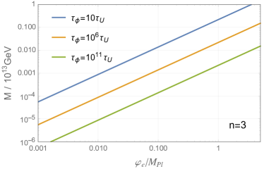
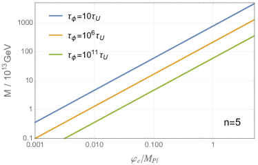
Figure 1: Dependence of the scalar $\phi$ mass $M$ on the inflaton field $\varphi_{e}$ at the end of inflation for a set of the DM lifetimes $\tau_{\phi}$ and coupling terms (16). The cases $n=3,4,5,6$ are shown on the top left, top right, bottom left and bottom right plots. We have set $w=0$ (matter-dominated evolution during preheating), $A=\frac{H_{e}}{M}$, and $T_{reh}=10^{15}~{}\mbox{GeV}$. The region above the blue line ($\tau_{\phi}=10\,\tau_{U}$) is excluded by the DM stability constraints. Recall, that we always assume that $H_{e}\lesssim M/5$. Since in a particular model $\varphi_{e}$ and $H_{e}$ are related, some regions on the plots may be unsuitable, if the inequality becomes invalid.

Cosmologically viable part of the model parameter space grows with the dimension of the inflaton coupling function $F(\varphi)$, as it is clearly seen from Fig. 1. In particular, for $n=4$, $M=10^{13}~{}\mbox{GeV}$, $\varphi_{e}=M_{Pl}$, $A=H_{e}/M$, and $T_{reh}=10^{15}~{}\mbox{GeV}$, one gets from Eq. (18): $\tau_{\phi}\approx 1.5\cdot 10^{12}\tau_{U}$, which is definitely consistent with the DM stability. The higher the operator dimension, the longer the DM lifetime in the model is.

Note that the stability at the time scale of the age of the present Universe is a necessary but not always a sufficient condition of viability of the model. DM couples to the inflaton, which in turn must couple to the SM particles to reheat the Universe. Hence, even rarely decaying DM contributes to the cosmic ray flux, which has been measured in a wide energy range up to $10^{11}$ GeV. A reasonable consistency of this flux with expectations from the astrophysical sources places limits on the decay rate of a heavy relic of a given mass depending on its decay pattern. Generically, the DM lifetime must exceed the age of the Universe by many orders of magnitude. Namely, $\tau_{DM}\gtrsim 10^{20-22}~{}\mbox{years}$ for $M\simeq 10^{13}~{}\mbox{GeV}$, if the decay initiates a noticeable energy release into gamma rays or neutrinos, see, e.g., Ref. [25, 30]. This requirement (if applicable) is consistent with our mechanism for integer $n>3$ (non-renormalizable interaction (16)), including inflationary models predicting potentially observable tensor modes. The renormalizable model with $n=3$ in Eq. (16) is consistent only for small Hubble inflation. So, no detectable relic gravitational waves are expected in that case.

The value $\varphi_{e}\simeq M_{Pl}$ is typical in monomial large field inflation, where the inflaton is minimally coupled to gravity. Generically, however, the inflaton may substantially deviate from the Planckian value. An example of this situation is exhibited in the Higgs inflation [36, 37, 38]—one of currently favored models. At the end of inflation, the Higgs field defined in the Jordan frame has the value $\varphi_{e}\simeq\frac{M_{Pl}}{5\sqrt{\xi}}$, where $\xi$ measures the non-minimal coupling to gravity; typically $\xi\sim 10^{4}$; we set $\varphi_{e}=M_{Pl}/500$. Taking $M=5\cdot 10^{13}~{}\mbox{GeV}$ and $T_{reh}=10^{15}~{}\mbox{GeV}$ [33], we get from Eq. (18): $\tau_{\phi}\approx 60~{}\tau_{U}$, $\tau_{\phi}\approx 10^{10}~{}\tau_{U}$, and $\tau_{\phi}\approx 2\cdot 10^{18}~{}\tau_{U}$ for $n=6,7,8$, respectively. We see that consistency with cosmic rays propagation requires rather high dimension operators, $n\geq 7$, in the case of Higgs inflation.

So far, we mainly discussed very heavy DM, $M\gtrsim 10^{13}~{}\mbox{GeV}$, being interested in inflationary models with detectable relic gravitational waves which amplitude at production is $\propto H_{e}/M_{Pl}$. However, with the current null result in searches of primordial gravitational waves, it is legitimate to consider inflation with a low expansion rate $H$ and masses $M\ll 10^{13}~{}\mbox{GeV}$. Then any couplings to the inflaton given by Eq. (16), including the renormalizable one, $n=3$, become consistent with the cosmic ray observations. In this regard, the region $M\lesssim 10^{9}~{}\mbox{GeV}$ corresponding to the lifetime $\tau_{\phi}\simeq 10^{11}-10^{12}\tau_{U}$ can be of particular interest from the viewpoint of IceCube neutrino observations [39, 40]. Namely, if the inflaton mainly decays into leptons, one can explain the origin of PeV neutrinos without spoiling Fermi limits on the gamma rays [30] obtained in Refs. [29, 31]. Note that the region of interest corresponds to relatively small values of the inflaton at the end of inflation: $\varphi_{e}\lesssim 0.1M_{Pl}$ in the renormalizable case $n=3$. Even smaller values of $\varphi_{e}$ are required for $n>3$.

We finish this Section with two concluding remarks. First, let us estimate the typical value of the coupling constant $\alpha$. Taking $M=10^{13}~{}\mbox{GeV}$, $\varphi_{e}=M_{Pl}$, and $T_{reh}=10^{15}~{}\mbox{GeV}$ and assuming $\Lambda=M_{Pl}$ in Eq. (16), we get from Eq. (11)

$$\alpha\approx 0.3\cdot 10^{-24}\;.$$ (21)

Thus, our mechanism implies extremely feeble interactions with the inflation.

Second, for fixed $\tau_{\phi}/\tau_{U}$ and $\varphi_{e}$, one can estimate the maximal possible value of $M$ achieved in the limit $n\rightarrow\infty$ (both Eqs. (18) and (19) give the same result):

$$\frac{M}{10^{13}~{}\mbox{GeV}}\simeq 10^{7}\;\sqrt{n}\cdot\frac{\varphi_{e}}{M_{Pl}}\;.$$

Hence, for the large field inflation, there is essentially no upper bound on the mass of the field $\phi$ produced. Say, $M=M_{Pl}$, the largest mass allowed within the quantum field theory at our present understanding of gravity, is achieved with $n\approx 18$ for $\varphi_{e}=M_{Pl}$ and $\tau_{\phi}\sim 10^{12}\cdot\tau_{U}$. This implies that the decaying DM can contribute to the cosmic rays starting from the Planckian energies, that may be observed (at least in the neutrino sector, where the energy does not degrade).

4 Scenario with subsequent decay to lighter particles

In the rest of the paper, we discuss a variation of our basic scenario assuming that the superheavy fields are unstable, while the ”true” DM particles appear as their decay products. This is the only viable option in the inflationary scenarios with inherently short lifetime of particles $\phi$.

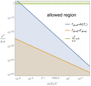
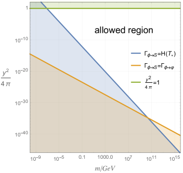
Figure 2: The plots show allowed values of the coupling constant $\frac{y^{2}}{4\pi}$ and the DM mass $m$ in the scenario, where the superheavy field $\phi$ produced during inflation subsequently decays to a couple of stable Dirac fermions. We have set $w=0$ (matter-dominated evolution right after inflation), $\varphi_{e}=M_{Pl}$, $T_{reh}=10^{15}~{}\mbox{GeV}$, $A=H_{e}/M$. For the field $\phi$ mass we put $M=10^{14}~{}\mbox{GeV}$ (left plot) and $M=10^{16}$ GeV (right plot). The light blue regions correspond to cosmologically unacceptable hot DM.

We assume that the field $\phi$ has an additional Yukawa coupling to the Dirac fermion $S$ of the mass $m$ — a singlet with respect to the SM gauge group,

$${\cal L}=y\phi\bar{S}S\,,$$ (22)

where $y$ is a dimensionless Yukawa coupling. The Dirac fermion is stable and serves as DM. In this picture, the concentration of DM particles is still fixed by the inflationary dynamics, and it is twice that of the particle $\phi$:

$$n_{DM}=\frac{A^{2}F^{2}(\varphi_{e})}{M^{3}}\cdot\left(\frac{a_{e}}{a}\right)^{3}\;.$$ (23)

The energy density of DM is then given by $\rho_{DM}=m\cdot n_{DM}$. The condition that it constitutes (almost) all of the invisible matter in the Universe reads

$$\frac{8\pi\,h_{*}(T_{eq})\,A^{2}\,F^{2}_{e}\,T_{reh}}{3\,g_{*}(T_{eq})\,M^{2}\,H^{2}_{e}\,M^{2}_{Pl}\,T_{eq}}\cdot\frac{m}{M}\approx 1\;,$$ (24)

where we have chosen the scenario with the matter dominated evolution right after inflation, cf. Eq. (11). Note that in this version of the mechanism the coupling constant of the scalar $\phi$ to the inflaton can be substantially larger compared to the estimate (21) by the factor $\sqrt{M/m}$.

The particles $S$ produced in the decays of the scalar $\phi$ generically have very high momenta $\simeq M/2$ at the moment of decay. On the other hand, DM particles must be very non-relativistic at the matter-radiation equality: the velocity of DM fluid should not exceed $v\simeq 10^{-3}$. Otherwise, a well established picture of the large scale structure formation would be spoiled. In order to fulfill this condition, the particles $S$ must become non-relativistic at least by the time, when the Universe cools down to $T\simeq 1~{}\mbox{keV}$. Hence, the scalar $\phi$ should decay into the particles $S$ before the Universe temperature reaches

$$T_{*}=\left(\frac{M}{2m}\right)\times 1\;\text{keV}\;.$$

That is, the following condition must be obeyed:

$$\Gamma_{\phi\rightarrow S}\gg H(T_{*})=\sqrt{\frac{8\pi^{3}g_{*}(T_{*})}{90}}\cdot\frac{T^{2}_{*}}{M_{Pl}}\;.$$ (25)

Furthermore, the decay rate into $S$-particles must exceed that into the inflatons, i.e.,

$$\Gamma_{\phi\rightarrow\varphi}\ll\Gamma_{\phi\rightarrow S}\;.$$ (26)

If there is the decay in two light particles, as it is suggested by Eq. (22), then its rate is given by

$$\Gamma_{\phi\rightarrow S}=\frac{y^{2}M}{8\pi}\,.$$

The decay rate $\Gamma_{\phi\rightarrow\varphi}$ is inferred from Eq. (17). We assume the renormalizable interaction with the inflaton, i.e., $n=3$. The conditions Eqs. (25) and (26) can be interpreted as the constraints on the coupling constant $y$:

$$2\cdot 10^{-26}\cdot\sqrt{\frac{g_{*}(T_{*})}{10}}\cdot\left(\frac{M}{10^{13}~{}\mbox{GeV}}\right)\cdot\left(\frac{10~{}\mbox{TeV}}{m}\right)^{2}\ll\frac{y^{2}}{4\pi}\ll 1\;,$$ (27)

and

$$\frac{y^{2}}{4\pi}\gg 3\cdot 10^{-41}\cdot\left(\frac{H_{e}}{M\cdot A}\right)^{2}\cdot\left(\frac{M}{10^{13}~{}\mbox{GeV}}\right)^{5}\cdot\left(\frac{M_{Pl}}{\varphi_{e}}\right)^{6}\cdot\left(\frac{10^{12}~{}\mbox{GeV}}{T_{reh}}\right)\cdot\frac{10~{}\mbox{TeV}}{m}\;.$$ (28)

None of the above constraints is particularly restrictive leaving a broad range of possible values of the coupling constant $y$ for fairly arbitrary masses $m$, as is shown in Fig. 2. Interestingly, when the value of $y^{2}/4\pi$ is close to its lower bound in the inequality (27), warm DM is produced. This is despite the fact that the DM particles can be heavy, well above $\sim\mbox{keV}$, cf. Ref. [41]. Note that we again assume the estimate (20) for the coefficient $A$. More generic powerlaw dependence of the coefficient $A$ is not expected to change the picture dramatically. However, if $A$ decreases exponentially with $M$, the present analysis should be revisited.

5 Discussions

We studied in detail a novel mechanism of producing superheavy DM in the form of the scalar field $\phi$ condensate. For any given inflationary model and the coupling of the field $\phi$ to the inflaton, the DM decay rate can be calculated, and the results can be contrasted with the existing data on the propagation of the cosmic rays. The choice of dataset one should use depends on the composition of cosmic rays originating from the decays of the inflaton. In turn, the composition depends on the interaction of the inflaton with the SM particles, responsible for the reheating in the early Universe.

For the simplest possible couplings of the field $\phi$ to the inflaton, our mechanism is very predictive, allowing to exclude a set of inflationary scenarios (provided that the mechanism works), or strongly constrain the range of DM masses. For example, the renormalizable interaction is only marginally consistent with the DM stability constraint, $\tau_{DM}\gtrsim 10^{10}~{}\mbox{years}$, in the high scale inflationary scenarios with the Hubble rate $H\simeq 10^{13-14}~{}\mbox{GeV}$. Hence, possible future observation of gravitational waves will strongly corner this option. The parameter space is broader in the case of non-renormalizable interactions.

On the other hand, if searches for tensor modes show null result, the window for possible masses $M$ is essentially unbounded from below. The typical DM lifetime can be very large in that case. If $\tau_{\phi}\gtrsim 10^{20-22}~{}\mbox{years}$, one can entertain the opportunity that a fraction of the observed very high energy neutrinos and gamma-rays originate from the decays of DM.

More generally, the scenario considered in the present work, can be viewed as a mechanism of generating superheavy fields—not necessarily DM. Subsequent decays of these fields may source DM in the form of some lighter stable particles from the Standard Model extensions, e.g., sterile neutrinos. Alternatively, these fields can be used for creating baryon asymmetry in the Affleck–Dine fashion [17]. This opens up the opportunity of unified description of DM production and baryogenesis.

Appendix

In the present Appendix, our goal is to estimate the coefficient $A$ entering Eq. (5) using different toy examples. We simplify the problem by switching off the Hubble friction in Eq. (2). Then, the equation, which describes the evolution of the field $\phi$ is given by

$$\ddot{\phi}+M^{2}\phi=F(t)\;.$$

The Hubble friction serves to set the tracking solution for the field $\phi$ during inflation. However, the same can be achieved by tuning initial conditions:

$$\phi=\frac{F(\varphi)}{M^{2}}\qquad\dot{\phi}=\frac{\dot{F}(\varphi)}{M^{2}}\qquad(t\rightarrow-\infty)\;.$$ (29)

It is convenient to split the solution for $\phi$ in two parts:

$$\phi=\frac{F}{M^{2}}+\chi\;,$$

The first term on the r.h.s. decays together with the inflaton. We are interested in the second term, $\chi$, which is relevant for the observed abundance of DM in our picture. The field $\chi$ satisfies the equation:

$$\ddot{\chi}+M^{2}\chi=-\frac{\ddot{F}}{M^{2}}\;.$$

This equation is to be solved with the trivial initial conditions: $\chi(t\rightarrow-\infty)=0$ and $\dot{\chi}(t\rightarrow-\infty)=0$, which match (29). The result reads:

$$\chi=\frac{\cos(Mt)}{M^{3}}\cdot\int^{t}_{-\infty}dt^{\prime}\sin(Mt^{\prime})\ddot{F}(t^{\prime})-\frac{\sin(Mt)}{M^{3}}\cdot\int^{t}_{-\infty}dt^{\prime}\cdot\cos(Mt^{\prime})\ddot{F}(t^{\prime})\;.$$ (30)

We are interested in large times $t$, when $F(\varphi)\rightarrow 0$ and consequently $\phi\rightarrow\chi$. In this limit, one can also replace the limits of integration by $\infty$. One gets

$$\phi(t)=\frac{\cos(Mt)}{M^{3}}\cdot\int^{+\infty}_{-\infty}dt^{\prime}\sin(Mt^{\prime})\ddot{F}(t^{\prime})-\frac{\sin(Mt)}{M^{3}}\cdot\int^{+\infty}_{-\infty}dt^{\prime}\cdot\cos(Mt^{\prime})\ddot{F}(t^{\prime})\;.$$ (31)

This is the field value, which feeds into the observed abundance of DM. We see that it is never zero generically. The value of the coefficient $A$ can be read off from Eq. (31) by the comparison with Eq. (5). We see that $A$ is defined by the Fourier transform of the function $\ddot{F}$. We have no a priori expectations about the $M$-dependence of the Fourier transform. However, the examples below point out that the coefficient $A$ i) drops exponentially with $M$ for a smooth slow evolution of the inflaton including its derivatives; ii) has a powerlaw dependence on $M$, if some derivatives of the inflaton change very fast on the time scale $M^{-1}$.

Exponential behavior of $A$. To illustrate the former situation, let us choose the function $F$ as follows:

$$F(t)=\Lambda^{3}\left[\frac{1}{2}-\frac{1}{\pi}\arctan(mt)\right]\;,$$

where $\Lambda$ and $m$ are two parameters of the mass dimension. In the limit $t\rightarrow-\infty$ one has $F(t\rightarrow-\infty)=\Lambda^{3}=\mbox{const}$, and at $t\rightarrow+\infty$ one has $F(t)\rightarrow 0$. Hence, this function $F$ correctly captures dynamics of the inflaton, which is nearly constant initially and then decays at the post-inflationary epoch. The second derivative of the function $F$ is given by

$$\ddot{F}=\frac{2m^{3}\Lambda^{3}t}{\pi\left[(1+(mt)^{2}\right]^{2}}\;.$$

One calculates the integrals in Eq. (30) using Jordan’s lemma. The result reads

$$\phi(t)=\frac{\Lambda^{3}\cdot\cos(Mt)}{M^{2}}\cdot e^{-\frac{M}{m}}\;.$$

Comparing with Eq. (5), we obtain finally

$$A=2\cdot e^{-\frac{M}{m}}\;.$$

Hence, the coefficient is of order one for an abrupt change, $m\gtrsim M$ or exponentially small for slow evolution, $m\ll M$.

Powerlaw behavior of $A$. Now let us consider the situation, when the $n$-th derivative of the function $F(t)$ changes abruptly, so that $F^{(n+1)}\propto\delta(t)$. In practice, it is enough, if $F^{(n+1)}$ changes fast on the times scales $M^{-1}$. In this situation, by integrating Eq. (31) by parts, we get

$$\phi(t)=\frac{\cos(Mt+\delta)}{M^{n+2}}\cdot F^{(n)}(0)\;,$$

where $\delta$ is an irrelevant phase. Comparing with Eq. (5), we read off the coefficient $A$:

$$A\simeq\frac{F^{(n)}(0)}{M^{n}\cdot F(0)}\;.$$ (32)

Now let us support the estimate (32) using an example, which incorporates the effects of the Hubble friction. It is easy to model the situation, where the first derivative of the inflaton undergoes a discontinuous jump. For this purpose, we choose the inflaton profile as follows

$$\varphi=\varphi_{e}=\mbox{const}~{}(t<t_{e})\qquad\varphi=\varphi_{e}\cdot\left(\frac{a_{e}}{a}\right)^{3/2}\;.$$ (33)

Namely, inflation is approximated by the exact de Sitter stage followed by the post-inflationary epoch with the equation of state $w=0$ and the scale factor $a(t)\propto t^{2/3}$. During the matter-dominated stage, the exact general solution for the field $\phi(t)$ can be written as

$$\phi(t)=-\frac{\cos(Mt)}{a^{3/2}(t)}\cdot\int dt\frac{\sin(Mt)}{M}F(\varphi)a^{3/2}(t)+\frac{\sin(Mt)}{a^{3/2}}\cdot\int dt\frac{\cos(Mt)}{M}F(\varphi)a^{3/2}(t)\;.$$

Up until the times $t=t_{e}$, the field $\phi$ tracks the inflaton, so that its initial conditions at the onset of the post-inflationary decay are given by

$$\phi(t_{e})=\frac{F(\varphi_{e})}{M^{2}}\qquad\dot{\phi}(t_{e})=0\;.$$ (34)

As in the bulk of the paper, we assume that $F(\varphi)$ is a powerlaw, i.e., $F(\varphi)\propto\varphi^{n}$. Now we are ready to write down the solution, which satisfies the initial conditions (34):

$$\begin{split}\phi&=\frac{F_{e}\cos\xi}{M^{2}}\cdot\frac{Mt_{e}}{Mt_{e}+\xi}\cdot\left[1-\int^{\xi}_{0}d\xi^{\prime}\frac{(Mt_{e})^{n-1}\sin\xi^{\prime}}{(Mt_{e}+\xi^{\prime})^{n-1}}\right]+\\ &+\frac{F_{e}\sin\xi}{M^{2}}\cdot\frac{Mt_{e}}{Mt_{e}+\xi}\cdot\left[\int^{\xi}_{0}d\xi^{\prime}\cdot\frac{(Mt_{e})^{n-1}\cos\xi^{\prime}}{(Mt_{e}+\xi^{\prime})^{n-1}}+\frac{1}{Mt_{e}}\right]\;,\end{split}$$

where $\xi\equiv M(t-t_{e})$. For the sake of concreteness, we focus on the case $F(\varphi)\propto\varphi^{2}$. We use the fact that the integrals over $\xi$ are converging fast, and thus can be replaced by their values at large $\xi$:

$$\int^{\infty}_{0}d\xi^{\prime}\cdot\frac{Mt_{e}\cos\xi^{\prime}}{Mt_{e}+\xi^{\prime}}=\frac{1}{Mt_{e}}\qquad\int^{\infty}_{0}d\xi^{\prime}\cdot\frac{Mt_{e}\sin\xi^{\prime}}{Mt_{e}+\xi^{\prime}}=1+{\cal O}\left(\frac{1}{[Mt_{e}]^{2}}\right)\;.$$ (35)

Hence, the solution of interest reads

$$\phi(t\gg t_{e})=\frac{2F_{e}}{M^{3}t_{e}}\cdot\left(\frac{a_{e}}{a}\right)^{3/2}\cdot\sin[M(t-t_{e})]\;.$$ (36)

Comparing the latter with Eq. (5), we get for the coefficient $A$:

$$A=\frac{2}{Mt_{e}}\simeq\frac{H_{e}}{M}\;.$$

This is a cross-check of Eq. (32) and justification of Eq. (20). We have checked that this result is robust against different choices of the function $F(\varphi)$ (still, powerlaw in $\varphi$). Furthermore, we have also considered the situation, when the 2-nd derivative of the inflaton experiences a discontinuous jump, while the $0$-th and the $1$-st ones are smooth. In that case, one gets $A\simeq H^{2}_{e}/M^{2}$ in agreement with Eq. (32).

References

- [1] D. J. H. Chung, E. W. Kolb and A. Riotto, Phys. Rev. D 59 (1999) 023501 doi:10.1103/PhysRevD.59.023501 [hep-ph/9802238].
- [2] V. Kuzmin and I. Tkachev, JETP Lett. 68 (1998) 271 [Pisma Zh. Eksp. Teor. Fiz. 68 (1998) 255] doi:10.1134/1.567858 [hep-ph/9802304].
- [3] V. Kuzmin and I. Tkachev, Phys. Rev. D 59 (1999) 123006 doi:10.1103/PhysRevD.59.123006 [hep-ph/9809547].
- [4] A. A. Grib and S. G. Mamaev, Yad. Fiz. 10 (1969) 1276 [Sov. J. Nucl. Phys. 10 (1970) 722].
- [5] L. Parker, Phys. Rev. 183 (1969) 1057. doi:10.1103/PhysRev.183.1057
- [6] Y. B. Zeldovich and A. A. Starobinsky, Sov. Phys. JETP 34 (1972) 1159 [Zh. Eksp. Teor. Fiz. 61 (1971) 2161].
- [7] S. G. Mamaev, V. M. Mostepanenko and A. A. Starobinsky, Zh. Eksp. Teor. Fiz. 70 (1976) 1577.
- [8] D. J. H. Chung, E. W. Kolb and A. Riotto, Phys. Rev. Lett. 81 (1998) 4048 doi:10.1103/PhysRevLett.81.4048 [hep-ph/9805473].
- [9] B. R. Greene, T. Prokopec and T. G. Roos, Phys. Rev. D 56 (1997) 6484 doi:10.1103/PhysRevD.56.6484 [hep-ph/9705357].
- [10] V. A. Kuzmin and V. A. Rubakov, Phys. Atom. Nucl. 61 (1998) 1028 [astro-ph/9709187].
- [11] D. J. H. Chung, E. W. Kolb and A. Riotto, Phys. Rev. D 60 (1999) 063504 doi:10.1103/PhysRevD.60.063504 [hep-ph/9809453].
- [12] D. S. Gorbunov and A. G. Panin, Phys. Lett. B 700 (2011) 157 doi:10.1016/j.physletb.2011.04.067 [arXiv:1009.2448 [hep-ph]].
- [13] V. A. Kuzmin and I. I. Tkachev, Phys. Rept. 320 (1999) 199 doi:10.1016/S0370-1573(99)00064-2 [hep-ph/9903542].
- [14] V. Berezinsky, M. Kachelriess and A. Vilenkin, Phys. Rev. Lett. 79 (1997) 4302 doi:10.1103/PhysRevLett.79.4302 [astro-ph/9708217].
- [15] V. Berezinsky, P. Blasi and A. Vilenkin, Phys. Rev. D 58 (1998) 103515 doi:10.1103/PhysRevD.58.103515 [astro-ph/9803271].
- [16] E. Babichev, D. Gorbunov and S. Ramazanov, Phys. Rev. D 97 (2018) no.12, 123543 doi:10.1103/PhysRevD.97.123543 [arXiv:1805.05904 [astro-ph.CO]].
- [17] E. Babichev, D. Gorbunov and S. Ramazanov, arXiv:1809.08108 [astro-ph.CO].
- [18] D. J. E. Marsh, Phys. Rept. 643 (2016) 1 doi:10.1016/j.physrep.2016.06.005 [arXiv:1510.07633 [astro-ph.CO]].
- [19] M. Cicoli, K. Dutta, A. Maharana and F. Quevedo, JCAP 1608 (2016) no.08, 006 doi:10.1088/1475-7516/2016/08/006 [arXiv:1604.08512 [hep-th]].
- [20] D. J. H. Chung, E. W. Kolb, A. Riotto and I. I. Tkachev, Phys. Rev. D 62 (2000) 043508 doi:10.1103/PhysRevD.62.043508 [hep-ph/9910437].
- [21] Y. Ema, K. Nakayama and Y. Tang, JHEP 1809 (2018) 135 doi:10.1007/JHEP09(2018)135 [arXiv:1804.07471 [hep-ph]].
- [22] D. J. H. Chung, E. W. Kolb, A. Riotto and L. Senatore, Phys. Rev. D 72 (2005) 023511 doi:10.1103/PhysRevD.72.023511 [astro-ph/0411468].
- [23] M. Ackermann et al. [Fermi-LAT Collaboration], Astrophys. J. 799 (2015) 86 doi:10.1088/0004-637X/799/1/86 [arXiv:1410.3696 [astro-ph.HE]].
- [24] M. G. Aartsen et al. [IceCube Collaboration], Phys. Rev. Lett. 113 (2014) 101101 doi:10.1103/PhysRevLett.113.101101 [arXiv:1405.5303 [astro-ph.HE]].
- [25] A. Esmaili, A. Ibarra and O. L. G. Peres, JCAP 1211 (2012) 034 doi:10.1088/1475-7516/2012/11/034 [arXiv:1205.5281 [hep-ph]].
- [26] R. Aloisio, S. Matarrese and A. V. Olinto, JCAP 1508 (2015) no.08, 024 doi:10.1088/1475-7516/2015/08/024 [arXiv:1504.01319 [astro-ph.HE]].
- [27] O. K. Kalashev and M. Y. Kuznetsov, Phys. Rev. D 94 (2016) no.6, 063535 doi:10.1103/PhysRevD.94.063535 [arXiv:1606.07354 [astro-ph.HE]].
- [28] L. Marzola and F. R. Urban, Astropart. Phys. 93 (2017) 56 doi:10.1016/j.astropartphys.2017.04.005 [arXiv:1611.07180 [astro-ph.HE]].
- [29] T. Cohen, K. Murase, N. L. Rodd, B. R. Safdi and Y. Soreq, Phys. Rev. Lett. 119 (2017) no.2, 021102 doi:10.1103/PhysRevLett.119.021102 [arXiv:1612.05638 [hep-ph]].
- [30] M. Kachelriess, O. E. Kalashev and M. Y. Kuznetsov, Phys. Rev. D 98 (2018) 083016 doi:10.1103/PhysRevD.98.083016 [arXiv:1805.04500 [astro-ph.HE]].
- [31] C. Blanco and D. Hooper, arXiv:1811.05988 [astro-ph.HE].
- [32] A. Ibarra, D. Tran and C. Weniger, Int. J. Mod. Phys. A 28 (2013) 1330040 doi:10.1142/S0217751X13300408 [arXiv:1307.6434 [hep-ph]].
- [33] F. Bezrukov, D. Gorbunov, C. Shepherd and A. Tokareva, arXiv:1904.04737 [hep-ph].
- [34] V. A. Rubakov and D. S. Gorbunov, doi:10.1142/10447
- [35] Y. Akrami et al. [Planck Collaboration], arXiv:1807.06211 [astro-ph.CO].
- [36] F. L. Bezrukov and M. Shaposhnikov, Phys. Lett. B 659 (2008) 703 doi:10.1016/j.physletb.2007.11.072 [arXiv:0710.3755 [hep-th]].
- [37] Y. Ema, Phys. Lett. B 770 (2017) 403 doi:10.1016/j.physletb.2017.04.060 [arXiv:1701.07665 [hep-ph]].
- [38] D. Gorbunov and A. Tokareva, Phys. Lett. B 788 (2019) 37 doi:10.1016/j.physletb.2018.11.015 [arXiv:1807.02392 [hep-ph]].
- [39] B. Feldstein, A. Kusenko, S. Matsumoto and T. T. Yanagida, Phys. Rev. D 88 (2013) no.1, 015004 doi:10.1103/PhysRevD.88.015004 [arXiv:1303.7320 [hep-ph]].
- [40] A. Esmaili, S. K. Kang and P. D. Serpico, JCAP 1412 (2014) no.12, 054 doi:10.1088/1475-7516/2014/12/054 [arXiv:1410.5979 [hep-ph]].
- [41] D. Gorbunov, A. Khmelnitsky and V. Rubakov, JCAP 0810 (2008) 041 doi:10.1088/1475-7516/2008/10/041 [arXiv:0808.3910 [hep-ph]].