Another proof of $p_{c}=\tfrac{\sqrt{q}}{1+\sqrt{q}}$ on $\mathbb{Z}^{2}$ with $q\in[1,4]$ for random-cluster model.

Abstract

In this paper we give another proof of $p_{c}=\tfrac{\sqrt{q}}{1+\sqrt{q}}$ for random-cluster model in $\mathbb{Z}^{2}$ for $q\in[1,4]$, based on the method of parafermionic observables.

1 Introduction

Consider a finite connected subgraph $\Omega$ of $\mathbb{Z}^{2}$ and denote the set of its edges by $E(\Omega)$, the set of its vertices by $V(\Omega)$ and the set of its faces by $F(\Omega)$. Let us also define its boundary vertices $\partial\Omega$ to be the set of vertices of $\Omega$ with one neighbour in $\mathbb{Z}^{2}\backslash\Omega$. An edge is called a boundary edge if its ends belong to $\partial\Omega$, otherwise, the edge is called an inner edge. Let us define a configuration $\omega$ as an element of the set $\{0,1\}^{E(\Omega)}$. An edge $e\in E(\Omega)$ is called open in $\omega$ if $\omega(e)=1$, it is called closed otherwise. We say that two points $x,y\in V(\Omega)$ are connected in $\omega$ if there is a path of open edges connecting them, this event is denoted by $x\longleftrightarrow y$. If we are allowed to use only open edges from $A\subset\Omega$, we use the notation $x\underset{A}{\longleftrightarrow}y$. A maximal set of vertices connected to each other is called a cluster.

The random-cluster model is a family of probability measures on $\{0,1\}^{E(\Omega)}$ introduced in 1969 by K. Fortuin and P. Kasteleyn [FK72, For72a, For72b] as a two-parametric generalisation of Bernoulli percolation. It depends on two parameters $p\in[0,1]$ and $q\in\mathbb{R}^{+}$ and defined as

$$\phi_{\Omega,p,q}^{\#}(\omega)=\frac{1}{Z^{\#}_{\Omega,p,q}}q^{k^{\#}(\omega)}\prod_{e\in E(\Omega)}p^{\omega(e)}(1-p)^{1-\omega(e)},$$ (1)

where the normalisation coefficient

$$Z_{\Omega,p,q}^{\#}=\sum_{w\in\{0,1\}^{E(\Omega)}}q^{k^{\#}(\omega)}\prod_{e\in E(\Omega)}p^{\omega(e)}(1-p)^{1-\omega(e)}$$ (2)

is called the partition function. The notation $k^{\#}(\omega)$ is defined as follows: if $\#=0$, then $k^{0}(\omega)$ is the number of clusters in $\omega$ and corresponds to the measure $\phi^{0}_{\Omega,p,q}(\omega)$ (in this case, we speak of the random-cluster measure with free boundary conditions), $k^{1}(\omega)$ is the number of clusters in $\omega$ when all boundary vertices belong to one cluster. Then, all clusters touching the boundary are counted as one. This measure is denoted $\phi^{1}_{\Omega,p,q}(\omega)$ and called the random-cluster measure with wired boundary conditions. It is also possible to define the random-cluster measure for any intermediate boundary conditions $\xi$.

We can define random-cluster measures on an infinite graph by taking the limit of measures $\lim_{i\rightarrow\infty}\phi^{0}_{G_{i},p,q}$ (resp. $\lim_{i\rightarrow\infty}\phi^{1}_{G_{i},p,q}$) where $G_{i}$ is an increasing sequence of finite graphs converging to the infinite graph (for example boxes of increasing size).

When $q=1$, all measures are equal to the product measure used in Bernoulli percolation. When $q$ tends to zero, the random-cluster measure converges to uniform measures on connected subgraphs, spanning trees or spanning forests depending on the behaviour of $p$ [Gri06].

An important property of the random-cluster model is its connection to Ising and Potts models. The Edward-Sokal coupling [ES88] is the most standard way to relate random-cluster model for some $p$ and integer $q\geq 2$ with the Potts model with $q$ colours and the inverse temperature $\beta$ such that $p=1-e^{-\beta}$, it was done by constructing a correspondence between their configurations. Many results about Ising and Potts models were found using this construction.

As Bernoulli percolation and the Ising and Potts models, the random-cluster model undergoes a phase transition. For any value of $q$, there exists $p_{c}=p_{c}(q)\in(0,1)$ such that for $p>p_{c}$ there is almost surely an infinite connected component for a configuration on $\mathbb{Z}^{2}$ with arbitrary boundary conditions. If $p<p_{c}$ there is no infinite connected component.

The exact value of $p_{c}(q)$ was one of the most important questions not only for the random-cluster model itself, but also for Potts and Ising models, where it gives the exact value of inverse critical temperature $\beta_{cr}$.

It was proven in 2012 by H. Duminil-Copin and V. Beffara [BDC12] that $p_{c}$ is equal to the self-dual point, which gives the relation $p=p^{*}=p_{c}$ between $p$ and the parameter $p^{*}$ on the corresponding dual graph (see Section 2.3). More precisely,

Theorem 1.

On $\mathbb{Z}^{2}$, we have that for every $q\geq 1$,

$$p_{c}(q)=p_{sd}(q)=\frac{\sqrt{q}}{1+\sqrt{q}}.$$ (3)

Both [BDC12] and alternative proofs of Theorem 1 given in [DM14] and [DRT17] use the crossing probabilities, i.e the probability of the rectangle of size $n\times\alpha n$ to be crossed in a horizontal direction. By generalisation of the Russo-Seymour-Welsh approach, this probability is bounded away from $0$ and $1$ independently on $n$. Also, both methods are strongly based on the FKG inequality, which bounds from below the probability for two different crossings to hold simultaneously by the product of probabilities for each of the crossings to hold independently of another one (see Section 2.2).

The approach used here does not use crossing probabilities and barely uses the FKG inequality. It is based on the method of parafermionic observables (see Section 2.4). This approach was used in other lattice models to deduce the critical point (for self-avoiding walks in [DS10] and [Gla14], for loop $O(n)$ models in [DGPS17]). For the random-cluster model, this method was used in the case $q\geq 4$ in [BDS15]. Also this method was applied in [Lis17] in a general case of Ising model with no translational invariance. Despite all this progress, the application of this method in the case of $q<4$ remained open until now.

The key idea of the proof is to bound the derivative of the probability to have a path from the middle of the box to the boundary or between two fixed points on the opposite boundary of the strip. That is why this approach can be used in the case where crossing probabilities cannot be bounded, or even when FKG does not hold. Also we hope that this technique could be useful to study models without invariance under translation.

The paper is organised as follows. Section 2 gives all definitions and statements required for the proof. In Section 3, Theorem 1 is proven in the simple case $q\in[1,3]$. The idea of the proof for $q\in(3,4]$ is slightly similar to the previous one, but requires an additional construction. The strategy of the proof is given in Section 4, and the proof is completed in Sections 5–9.

Acknowledgments

The authors thank Hugo Duminil-Copin for suggesting the problem and many fruitful discussions. The work was supported by the NCCR Swissmap.

2 Definitions and basic properties

2.1 Domain Markov property and finite energy property

The Domain Markov property states that the only influence that a configuration outside a graph $G$ has on a configuration inside $G$ is via induced boundary conditions. More formally, suppose we have $G\subset G^{\prime}$ and some boundary conditions $\xi^{\prime}$ on $G^{\prime}$ and let $\psi$ be a configuration on $G^{\prime}\backslash G$. Let us define the following boundary conditions: two boundary clusters are counted as one if they are connected in $\psi$ (including the connections in $\xi^{\prime}$). These boundary conditions are called induced by the configuration $\psi$ with boundary conditions $\xi^{\prime}$ and denoted $(\psi,\xi^{\prime})$. Then, for any configuration $\omega$ on $G^{\prime}$ and its restriction to $G$ denoted $\omega_{|G}$, the following property holds:

$$\phi_{G^{\prime},p,q}^{\xi^{\prime}}(\omega\,|\,\omega_{e}=\psi_{e}\text{ for all }e\in G^{\prime}\backslash G)=\phi_{G,p,q}^{(\psi,\xi^{\prime})}(\omega_{|G}).$$

The finite energy property allows one to compare configurations which differ only on finitely many edges. For any $\varepsilon\in(0,\tfrac{1}{2})$ and for any $q>1$, there exists a constant $c=c(\varepsilon,q)>0$ such that, for every configuration $\omega$ and $\omega^{\prime}$ differing only on $k$ edges

$$c^{-k}\leq\frac{\phi^{\xi}_{G,p,q}(\omega)}{\phi^{\xi}_{G,p,q}(\omega^{\prime})}\leq c^{k}$$

for any $G$, any boundary conditions $\xi$, any fixed $q$ and any $p\in(\varepsilon,1-\varepsilon)$.

Let us use the notation $\omega^{e}$ (resp. $\omega_{e}$) for the configuration obtained from the configuration $\omega$ by setting the edge $e$ to be open (resp. close). Then for a fixed value of $p$, this property can also be written in the following way:

$$\frac{p}{q(1-p)}\leq\frac{\phi_{G,p,q}^{\xi}(\omega^{e})+\phi_{G,p,q}^{\xi}(\omega_{e})}{\phi_{G,p,q}^{\xi}(\omega_{e})}\leq\frac{p}{(1-p)}$$ (4)

for any $G,p,\xi$ and any $q\geq 1$.

2.2 Increasing events

The event $A$ is called increasing if for any edge $e$ and any configuration $\omega$ the fact that $A$ holds for $\omega_{e}$ implies that $A$ holds for $\omega^{e}$. If $A$ and $B$ are two increasing events, then the following inequality, called FKG inequality [FKG71], holds for any values of $p\in[0,1]$, $q\geq 1$ and for any graph $G$ and boundary condition $\xi$:

$$\phi^{\xi}_{G,p,q}(A\cap B)\geq\phi^{\xi}_{G,p,q}(A)\phi^{\xi}_{G,p,q}(B).$$ (5)

Let us now turn to the comparison between different boundary conditions. Write $\xi\geq\chi$ if any two boundary points seen as parts of one cluster in $\chi$ have the same property in $\xi$. Then, for any increasing $A$ and any $G,p$ and $q\geq 1$,

$$\phi^{\xi}_{G,p,q}(A)\geq\phi^{\chi}_{G,p,q}(A).$$ (6)

This inequality, together with the definition of induced boundary conditions, can be used to compare the measures in different domains. For example, if $G\subset G^{\prime}$ and $A$ is defined on $G$, then

$$\phi^{1}_{G,p,q}(A)\geq\phi^{\xi}_{G^{\prime},p,q}(A)\geq\phi^{0}_{G,p,q}(A)$$ (7)

for any $p,q\geq 1$ and any $\xi$.

The edge $e$ is called pivotal for the event $A$ in a given configuration $\omega$ if $A$ holds for $\omega^{e}$ and does not hold for $\omega_{e}$. Note that the fact that the edge is pivotal does not depend on the state of this edge in $\omega$. The following inequality holds for any increasing event $A$, boundary conditions $\xi$ and graph $G$ [Gri06]:

$$\frac{d}{dp}\phi^{\xi}_{G,p,q}(A)\geq c\sum_{e\in E(G)}\phi^{\xi}_{G,p,q}(e\text{ is pivotal for }A),$$ (8)

where $c$ does not depend on $G$, $A$ or $p$.

2.3 Duality

Let us define the dual lattice $L^{*}$ of a planar lattice $L$ as follows. The set of vertices of $L^{*}$ corresponds to the set $F(L)$ of faces of $L$ including the infinite face. In words, we put a vertex of the dual lattice in the middle of each face of $L$. Then, we connect all pairs of vertices corresponding to adjacent faces. Each edge of the dual lattice intersects exactly one edge of the primal lattice.

For a finite graph $G\subset L$, let $G^{*}$ denote the subgraph of $L^{*}$ with edges corresponding to edges of $G$ and vertices to the endpoints of these edges.

The configuration $\omega^{*}$ on $G^{*}$ dual to a configuration $\omega$ on $G$ is defined as follows:

$$\omega^{*}(e^{*})=1-\omega(e),$$

where $e$ is the edge of the primal lattice intersecting $e^{*}$. The probability of $\omega^{*}$ is set to be the probability of $\omega$. The event that $x$ is connected to $y$ by a dual-open path is denoted by $x\overset{*}{\longleftrightarrow}y$.

There exists a value $p^{*}=p^{*}(p,q)\in[0,1]$ such that the following relation is true [Gri06, Dum13]:

$$\phi^{\xi}_{G,p,q}(\omega)=\phi^{\xi^{*}}_{G^{*},p^{*},q}(\omega^{*}).$$ (9)

Here, $\xi^{*}$ denotes boundary conditions dual to $\xi$, for example wired boundary conditions are dual to free boundary conditions and vice versa. The value of $p^{*}$ is related to $p$ via the following equation:

$$\frac{pp^{*}}{(1-p)(1-p^{*})}=q.$$ (10)

As mentioned above, there exists the unique point $p_{sd}$ such that $p_{sd}=(p_{sd})^{*}$. Its value is equal to

$$p_{sd}=\frac{\sqrt{q}}{1+\sqrt{q}}.$$

2.4 Parafermionic observable

The medial lattice of a lattice $L$ is denoted by $L^{\diamond}$ and defined as follows. The set $V(L^{\diamond})$ corresponds to $E(L)$ (that can be interpreted as if we put a vertex in the middle of every edge of $L$). There is an edge between two vertices of $L^{\diamond}$ if the corresponding edges have one common end vertex and are adjacent to the same face. Note that the faces of $L^{\diamond}$ correspond to $V(L)\cup V(L^{*})$. We orient the edges of $L^{\diamond}$ counterclockwise around faces corresponding to vertices of $L$ (and, thus, clockwise around faces corresponding to vertices of $L^{*}$). Note that the lattice $(\mathbb{Z}^{2})^{\diamond}$ is a rescaled and rotated version of $\mathbb{Z}^{2}$.

The medial graph $G^{\diamond}$ of a finite graph $G\subset L$ is the subgraph of $L^{\diamond}$ made of all faces corresponding to the vertices of $G$ and $G^{*}$, all edges surrounding these faces and all vertices incident to these edges.

Let $\gamma$ be a path on $G^{\diamond}$ and let $e$ and $e^{\prime}$ be two edges belonging to $\gamma$. Then, the winding $W_{\gamma}(e,e^{\prime})$ is the total rotation done by $\gamma$ on the way from the middle of $e$ to the middle of $e^{\prime}$. If $e$ or $e^{\prime}$ do not belong to $\gamma$, we set $W_{\gamma}(e,e^{\prime})=0$.

Let us pick two vertices $a$ and $b$ on the boundary of $G$ and define Dobrushin boundary conditions, denoted $(a,b)$, as wired on the boundary arc from $a$ to $b$ clockwise and free for the rest of $\partial G$. Let us note that for dual configuration $(a,b)^{*}=(b,a)$. There is a primal cluster attached to the wired boundary part and a dual cluster attached to the free boundary part (in the dual configuration, it corresponds to a wired arc). The curve on the medial lattice going between these two clusters is called an exploration path (for more details, see [Dum13]). Note that it is oriented. Let us also add two edges $e_{a}$ and $e_{b}$ to begin and to end $\gamma$ outside of $G$, these edges are oriented according to the orientation rules stated above.

We follow [Smi10] and [DCST17] to define the parafermionic observable:

$$\hat{F}(e)=\hat{F}_{G,a,b,q,p_{sd}}(e)=\phi_{G,p_{sd},q}^{(a,b)}(e^{i\hat{\sigma}W_{\gamma}(e,e_{b})}\mathbb{I}_{e\in\gamma})\quad\forall e\in E(G^{\diamond}),$$

where $\gamma$ is the exploration path in $\omega$ and $\hat{\sigma}$ satisfies the following relation:

$$\cos(\tfrac{\hat{\sigma}\pi}{2})=\tfrac{\sqrt{q}}{2}.$$

Let us take any set $V\in V(G^{\diamond})$ such that any vertex $v\in V$ has four incident edges in $E(G^{\diamond})\cup\{e_{a},e_{b}\}$ and define its outer boundary

$$\delta V=\{e\in E(G^{\diamond})\cup\{e_{a},e_{b}\},\text{only one end of $e$ belongs to V}\}.$$ (11)

For edge $e\in\delta V$, define the function $\eta_{V}(e)$ to be equal to $1$ if $e$ is pointing to a vertex of $V$ and $-1$ otherwise. Then, the following property holds [DCST17]:

$$\sum_{e\in\delta V}\eta_{V}(e)\hat{F}(e)=0.$$ (12)

2.5 Graphs used in the proof

In this paper, we work on $\mathbb{Z}^{2}$ but also on other infinite graphs. The half-plane $\{(x,y)\in\mathbb{Z}^{2},y\geq 0\}$ is denoted by $\mathbb{H}$ (its boundary $\partial\mathbb{H}$ is equal to $\{(x,0)\in\mathbb{Z}^{2}\}$).

We can define the box of size $n$ in $\mathbb{Z}^{2}$ or in $\mathbb{H}$ as follows:

$$\Lambda_{n}=\{(x,y)\in\mathbb{Z}^{2}\text{(or $\mathbb{H}$)}:\max(|x|,|y|)\leq n\},$$

its boundary is naturally defined as

$$\partial\Lambda_{n}=\{(x,y)\in\mathbb{Z}^{2}\text{(or $\mathbb{H}$)}:\max(|x|,|y|)=n\}.$$

Free and wired boundary conditions are defined for $\mathbb{H}$ in the same way, as for $\mathbb{Z}^{2}$, as a limit of measures defined for boxes $\Lambda_{n}\subset\mathbb{H}$ with free (resp. wired) boundary conditions on $\partial\Lambda_{n}$ and on $\partial\mathbb{H}$. Also we work with $0\backslash 1$ boundary conditions, obtained by taking a limiting measure for boxes $\Lambda_{n}$ with Dobrushin $((0,n),(0,0))$ boundary conditions (see Section 2.4).

The strip of height $n$ in $\mathbb{Z}^{2}$ (which can also be seen as a strip in $\mathbb{H}$) is defined as:

$$S_{n}=\{(x,y)\in\mathbb{Z}^{2}:y\in[0,n]\}.$$

Let us call the left and the right parts of its boundary the subsets defined as:

$$\partial^{+}S_{n}=\{(x,y)\in\mathbb{Z}^{2}:y\in\{0,n\},x\geq 0\},$$

$$\partial^{-}S_{n}=\{(x,y)\in\mathbb{Z}^{2}:y\in\{0,n\},x\leq 0\}.$$

The bottom left part of $\partial S_{n}$ will be denoted by

$$\partial_{b}^{-}S_{n}=\{(x,0)\in\mathbb{Z}^{2}:x<0\}.$$

Free, wired or $0\backslash 1$ boundary condition measures on $S_{n}$ are defined as a limit of measures on rectangles $\{(x,y)\in\mathbb{Z}^{2}:x\in[-m,m],y\in[0,n]\}$ with free, wired or $((0,n),(0,0))$ boundary conditions respectively.

For some lemmas, we work on the universal cover of $\mathbb{Z}^{2}\backslash F_{0}$ where $F_{0}$ is the face $[0,1]\times[-1,0]$. The universal cover $\mathbb{U}$ is a graph defined as follows:

$$V(\mathbb{U})=\{ (x,y,z),x,y,z\in\mathbb{Z}\}=V(\mathbb{Z}^{3}),$$

$$E(\mathbb{U})=\{ ((x,y,z),(x,y+1,z))\,\forall x,y,z\in\mathbb{Z}\}$$

$$\cup\,\{ ((x,y,z),(x+1,y,z))\,\forall x,y,z\in\mathbb{Z}\text{ such that }x\neq 0\}$$

$$\cup\,\{ ((0,y,z),(1,y,z))\,\forall y,z\in\mathbb{Z}\text{ such that }y\geq 0\}$$

$$\cup\,\{ ((0,y,z),(1,y,z+1))\,\forall y,z\in\mathbb{Z}\text{ such that }y\leq 0\}.$$

We also introduce the truncated universal cover $\mathbb{U}_{k}$ to be the subgraph of $\mathbb{U}$ with vertices of the type $(x,y,z)$ with $|z|\leq k$. Let us define its boundary $\partial\mathbb{U}_{k}$ as $\{(0,-y,-k),y\in\mathbb{N}\}\cup\{(0,-y,k),y\in\mathbb{N}\}$.

We can define the analogue of a box $\Lambda_{n}$ in $\mathbb{U}_{k}$ as follows:

$$\Lambda_{n,k} =\{(x,y,z)\in\mathbb{U}_{k}:\max(|x|,|y|)\leq n\},$$

$$\partial\Lambda_{n,k} =\{(x,y,z)\in\mathbb{U}_{k}:\max(|x|,|y|)=n\}.$$

Free and wired boundary conditions are defined for $\mathbb{U}_{k}$ in the same way as for $\mathbb{Z}^{2}$. Let us also note that we can extend the notions of dual and medial graphs to $\mathbb{U}_{k}$.

3 Proof of Theorem 1 for $1\leq q\leq 3$.

The proof is simpler when $q\leq 3$. We therefore begin by discussing this case. Let us first notice that, by Zhang argument (see [Gri06]),

$$p_{c}\geq p_{sd}.$$ (13)

We therefore have to show only the inequality $p_{c}\leq p_{sd}$.

Let us take a set $S$ such that $S\subset\Lambda_{n}\subset\mathbb{Z}^{2}$ and $0\in S$ and define its edge boundary $\Delta S=\{(x,y)\in E(\Lambda_{n}):x\in S,y\not\in S\}$. Then, define the following auxiliary function:

$$\varphi_{p,q,n}(S)=\sum_{(x,y)\in\Delta S}{\phi_{S,p,q}^{0}[0\longleftrightarrow x]}.$$ (14)

The result is the consequence of the following two lemmas.

Lemma 2.

Let $p\geq p_{sd}$, $q>1$ and $n\geq 1$. Then, for any $G$ such that $\Lambda_{n}\subset G\subset\mathbb{Z}^{2}$, we have that

$$\frac{d}{dp}\phi_{G,p,q}^{\xi}[0\longleftrightarrow\partial\Lambda_{n}]\geq\frac{c}{1-p}\left(\inf_{S:\,0\in S\subset\Lambda_{n}}\varphi_{p,q,n}(S)\right)(1-\phi_{G,p,q}^{\xi}[0\longleftrightarrow\partial\Lambda_{n}])$$ (15)

where $c$ does not depend on $p,G$ or $\xi$.

Proof.

In this proof, we follow [DT16, DCT16]. The differential inequality (15) is a consequence of (4), (8) and the characterisation of pivotal edges:

$$\frac{d}{dp}\phi_{G,p,q}^{\xi}[0\longleftrightarrow\partial\Lambda_{n}]\geq\frac{c}{1-p}\!\!\sum_{e\in E(G)}\!\phi_{G,p,q}^{\xi}[e\text{ is pivotal for }\{0\longleftrightarrow\partial\Lambda_{n}\}\text{ and }\{0\nleftrightarrow\partial\Lambda_{n}\}].$$

Let us call $\mathcal{S}$ the set $\{x\in\Lambda_{n}:x\nleftrightarrow\partial\Lambda_{n}\}$. The event $\{0\nleftrightarrow\partial\Lambda_{n}\}$ can be rewritten as $\{0\in\mathcal{S}\}$. Note that, when the event $\{0\longleftrightarrow\partial\Lambda_{n}\}$ does not occur, all the pivotal edges are closed and lie in $\Delta\mathcal{S}$. Then,

$$\frac{d}{dp}\phi_{G,p,q}^{\xi}[0\longleftrightarrow\partial\Lambda_{n}] \geq\frac{c}{1-p}\sum_{S:\,0\in S\subset\Lambda_{n}}\sum_{e\in E(G)}\!\phi_{G,p,q}^{\xi}[e\text{ is pivotal for }\{0\longleftrightarrow\partial\Lambda_{n}\},\mathcal{S}=S]$$

$$\geq\frac{c}{1-p}\sum_{S:\,0\in S\subset\Lambda_{n}}\sum_{x:(x,y)\in\Delta\mathcal{S}}\!\phi_{G,p,q}^{\xi}[\{0\underset{S}{\longleftrightarrow}x\},\mathcal{S}=S]$$

$$\geq\frac{c}{1-p}\sum_{S:\,0\in S\subset\Lambda_{n}}\!\varphi_{p,q,n}(S)\phi_{G,p,q}^{\xi}[\mathcal{S}=S]$$

where the last inequality follows from the Domain Markov property. Then, we can conclude that

$$\frac{d}{dp}\phi_{G,p,q}^{\xi}[0\longleftrightarrow\partial\Lambda_{n}] \geq\frac{c}{1-p}\left(\inf_{S:\,0\in S\subset\Lambda_{n}}\varphi_{p,q,n}(S)\right)\phi_{G,p,q}^{\xi}[0\in\mathcal{S}]$$

$$=\frac{c}{1-p}\left(\inf_{S:\,0\in S\subset\Lambda_{n}}\varphi_{p,q,n}(S)\right)(1-\phi_{G,p,q}^{\xi}[0\longleftrightarrow\partial\Lambda_{n}]).$$

∎

Lemma 3.

There exists $C>0$ such that for any $n\geq 1$ and $S$ such that $0\in S\subset\Lambda_{n}$,

$$\varphi_{p_{sd},q,n}(S)>C.$$ (16)

Proof.

Consider a set $S$ such that $0\in S\subset\Lambda_{n}$.

We can define the graph $\Lambda_{n}^{\prime}$ as a box $\Lambda_{n}$ with vertices $\{(0,k),1\leq k\leq n\}$ removed. Then, let us denote the connected component of $S$ that contains $0$ as $S_{0}$ and work with the domain $S_{0}^{\prime}=S_{0}\cap\Lambda_{n}^{\prime}$. Let us call $(0)$ the boundary conditions that are free everywhere. These boundary conditions can be seen as Dobrushin boundary conditions with the wired arc collapsed to one point (i.e. $a=b=0$). This observation allows to define the exploration path $\gamma$ for a configuration in this domain. Its beginning edge $e_{a}=\bigl{(}(0,\tfrac{1}{2}),(-\tfrac{1}{2},0)\bigr{)}$ is adjacent to the edge $e_{b}=\bigl{(}(\tfrac{1}{2},0),(0,\tfrac{1}{2})\bigr{)}$, so $\gamma$ forms a loop around $0$, which bounds the open cluster in $S_{0}^{\prime}$ that contains $0$.

Let us call $V$ the set of all vertices in $V((S_{0}^{\prime})^{\diamond})$ that have four incident edges in $E((S_{0}^{\prime})^{\diamond})\cup\{e_{a},e_{b}\}$, then, $\delta V$ defined as in (11) can be split into three parts: first, $\delta_{0}=\{e_{a},e_{b}\}$, second, the edges adjacent to the slit from the right and from the left (it can be written as $\delta_{1}=\delta_{1}^{+}\cup\delta_{1}^{-}$, where edges in $\delta_{1}^{+}$ are of the form $\bigl{(}(\tfrac{1}{2},k),(1,k+\tfrac{1}{2})\bigr{)}$ or $\bigl{(}(\tfrac{1}{2},k+1),(1,k+\tfrac{1}{2})\bigr{)}$ and edges in $\delta_{1}^{-}$ are of the form $\bigl{(}(-\tfrac{1}{2},k),(-1,k+\tfrac{1}{2})\bigr{)}$ or $\bigl{(}(-\tfrac{1}{2},k+1),(-1,k+\tfrac{1}{2})\bigr{)}$), third, other edges neighbouring the boundary of $(S_{0}^{\prime})^{\diamond}$.

Let us also look at the domain $\overline{S}$ defined as the reflection of $S$ with respect to the $y$-axis. We can define $\overline{S^{\prime}_{0}}$, $\overline{V},\overline{\delta V},\overline{\delta_{1}^{+}},\overline{\delta_{1}^{-}}$ and $\overline{\delta_{2}}$ in the same way as for $S$.

Then, (12) can be written as

$$\sum_{e\in\delta_{2}}\eta_{V}(e)\hat{F}_{S^{\prime}_{0}}(e)+\sum_{e\in\overline{\delta_{2}}}\eta_{\overline{V}}(e)\hat{F}_{\overline{S^{\prime}_{0}}}(e)+\sum_{e\in\delta_{1}\cup\delta_{0}}\eta_{V}(e)\hat{F}_{S^{\prime}_{0}}(e)+\sum_{e\in\overline{\delta_{2}}\cup\delta_{0}}\eta_{\overline{V}}(e)\hat{F}_{\overline{S^{\prime}_{0}}}(e)=0,$$

or

$$\bigl{|}\sum_{e\in\delta_{1}\cup\delta_{0}}\eta_{V}(e)\hat{F}_{S^{\prime}_{0}}(e)+\sum_{e\in\overline{\delta_{2}}\cup\delta_{0}}\eta_{\overline{V}}(e)\hat{F}_{\overline{S^{\prime}_{0}}}(e)\bigr{|}\leq\bigl{|}\sum_{e\in\delta_{2}}\eta_{V}(e)\hat{F}_{S^{\prime}_{0}}(e)\bigr{|}+\bigl{|}\sum_{e\in\overline{\delta_{2}}}\eta_{\overline{V}}(e)\hat{F}_{\overline{S^{\prime}_{0}}}(e)\bigr{|}.$$ (17)

The first term in the right part of (17) is bounded as follows:

$$\bigl{|}\sum_{e\in\delta_{2}}\eta_{V}(e)\hat{F}_{S^{\prime}_{0}}(e)\bigr{|} \leq\sum_{e\in\delta_{2}}|\hat{F}_{S^{\prime}_{0}}(e)|=\sum_{e\in\delta_{2}}|\phi_{S^{\prime}_{0},p,q}^{(0)}(e^{i\sigma W_{\gamma}(e,e_{b})}\mathbb{I}_{e\in\gamma})|$$

$$=\sum_{e\in\delta_{2}}\phi_{S^{\prime}_{0},p,q}^{(0)}(e\in\gamma)=2\sum_{x\in\partial S_{0}}\phi_{S^{\prime},p,q}^{0}(0\longleftrightarrow x),$$

because any boundary vertex corresponds to two edges from $\delta_{2}$ that do or do not belong to $\gamma$ simultaneously. The second term is bounded by the same value because of the symmetry between $S$ and $S^{\prime}$:

$$\bigl{|}\sum_{e\in\delta_{2}}\eta_{\overline{V}}(e)\hat{F}_{\overline{S^{\prime}_{0}}}(e)\bigr{|}\leq 2\sum_{x\in\partial\overline{S}_{0}}\phi_{\overline{S_{0}^{\prime}},p,q}^{0}(0\longleftrightarrow x)\leq 2\sum_{x\in\partial S_{0}}\phi_{S^{\prime},p,q}^{0}(0\longleftrightarrow x).$$

Together, this gives the following bound on the right part of (17):

$$\bigl{|}\sum_{e\in\delta_{2}}\eta_{V}(e)\hat{F}_{S^{\prime}_{0}}(e)\bigr{|}\!+\!\bigl{|}\sum_{e\in\overline{\delta_{2}}}\eta_{\overline{V}}(e)\hat{F}_{\overline{S_{0}^{\prime}}}(e)\bigr{|}\leq 4\!\!\!\sum_{x\in\partial S_{0}}\!\!\phi_{S^{\prime},p,q}^{0}(0\longleftrightarrow x)\leq 4\!\!\!\sum_{x\in\partial S_{0}}\!\!\phi_{S,p,q}^{0}(0\longleftrightarrow x).$$ (18)

Before writing the inequality for the right part of (17), let us define the vertices of $S^{\prime}_{0}$ and $\overline{S^{\prime}_{0}}$ adjacent to the slit:

$$\partial^{+}_{slit}=\{(1,k),1\leq k\leq n\}\cup S_{0},\quad\overline{\partial^{+}_{slit}}=\{(1,k),1\leq k\leq n\}\cup\overline{S_{0}},$$

$$\partial^{-}_{slit}=\{(1,k),1\leq k\leq n\}\cup S_{0},\quad\overline{\partial^{-}_{slit}}=\{(1,k),1\leq k\leq n\}\cup\overline{S_{0}}.$$

Each of these points corresponds to two edges of $\delta_{1}$ or $\overline{\delta_{1}}$. Then, the sums in the left part of (17) are written as follows:

$$\sum_{e\in\delta_{1}\cup\delta_{0}}\eta_{V}(e)\hat{F}_{S_{0}^{\prime}}(e)=(e^{i\hat{\sigma}\frac{3\pi}{2}}-1)+\sum_{x\in\partial^{+}_{slit}}\phi^{0}_{S^{\prime}_{0},p_{sd},q}(x\longleftrightarrow 0)(e^{-i\hat{\sigma}\pi}-e^{-i\hat{\sigma}\frac{\pi}{2}})$$

$$+\sum_{x\in\partial^{-}_{slit}}\phi^{0}_{S^{\prime}_{0},p_{sd},q}(x\longleftrightarrow 0)(e^{2\pi i\hat{\sigma}}-e^{i\hat{\sigma}\frac{5\pi}{2}}),$$

$$\sum_{e\in\overline{\delta_{2}}\cup\delta_{0}}\eta_{\overline{V}}(e)\hat{F}_{\overline{S^{\prime}_{0}}}(e)=(e^{i\hat{\sigma}\frac{3\pi}{2}}-1)+\sum_{x\in\overline{\partial^{+}_{slit}}}\phi^{0}_{\overline{S^{\prime}_{0}},p_{sd},q}(x\longleftrightarrow 0)(e^{-i\hat{\sigma}\pi}-e^{-i\hat{\sigma}\frac{\pi}{2}})$$

$$+\sum_{x\in\overline{\partial^{-}_{slit}}}\phi^{0}_{\overline{S^{\prime}_{0}},p_{sd},q}(x\longleftrightarrow 0)(e^{2\pi i\hat{\sigma}}-e^{i\hat{\sigma}\frac{5\pi}{2}}).$$

Because of the symmetry of $S^{\prime}_{0}$ and $\overline{S^{\prime}_{0}}$, these equations can be summed to give

$$\bigl{|}\sum_{e\in\delta_{1}\cup\delta_{0}}\eta_{V}(e)\hat{F}_{S^{\prime}_{0}}(e) +\sum_{e\in\overline{\delta_{2}}\cup\delta_{0}}\eta_{\overline{V}}(e)\hat{F}_{\overline{S^{\prime}_{0}}}(e)\bigr{|}=\bigl{|}2(e^{i\hat{\sigma}\frac{3\pi}{2}}-1)$$

$$+\sum_{x\in\partial^{+}_{slit}\cup\partial^{-}_{slit}}\phi^{0}_{S^{\prime}_{0},p_{sd},q}(x\longleftrightarrow 0)(e^{-\pi i\hat{\sigma}}-e^{-i\hat{\sigma}\frac{\pi}{2}}+e^{2\pi i\hat{\sigma}}-e^{i\hat{\sigma}\frac{5\pi}{2}})\bigr{|}$$

$$=\bigl{|}2(e^{i\hat{\sigma}\frac{3\pi}{2}}-1)+\sum_{x\in\partial^{+}_{slit}\cup\partial^{-}_{slit}}2\phi^{0}_{S^{\prime}_{0},p_{sd},q}(x\longleftrightarrow 0)(e^{i\hat{\sigma}\frac{\pi}{2}}-e^{\pi i\hat{\sigma}})\cos(\hat{\sigma}\tfrac{3\pi}{2})\bigr{|}$$

$$=2\bigl{|}e^{\pi i\hat{\sigma}}-e^{i\hat{\sigma}\frac{\pi}{2}}\bigr{|}\cdot\bigl{|}\bigl{(}(e^{i\hat{\sigma}\frac{\pi}{2}}+1+e^{-i\hat{\sigma}\frac{\pi}{2}})-\!\!\!\!\!\!\sum_{x\in\partial^{+}_{slit}\cup\partial^{-}_{slit}}\phi^{0}_{S^{\prime}_{0},p_{sd},q}(x\longleftrightarrow 0)\cos(\hat{\sigma}\tfrac{3\pi}{2})\bigr{)}\bigr{|}$$

$$=2\bigl{|}e^{i\hat{\sigma}\frac{\pi}{2}}\bigr{|}\cdot\bigl{|}e^{i\hat{\sigma}\frac{\pi}{2}}-1\bigr{|}\cdot\bigl{|}\bigl{(}1+2\cos(\hat{\sigma}\tfrac{\pi}{2})-\!\!\!\!\!\!\sum_{x\in\partial^{+}_{slit}\cup\partial^{-}_{slit}}\phi^{0}_{S^{\prime}_{0},p_{sd},q}(x\longleftrightarrow 0)\cos(\hat{\sigma}\tfrac{3\pi}{2})\bigr{)}\bigr{|}$$

$$=2\bigl{|}e^{i\hat{\sigma}\frac{\pi}{2}}-1\bigr{|}\cdot\bigl{|}\bigl{(}1+\sqrt{q}+\!\!\!\!\!\!\sum_{x\in\partial^{+}_{slit}\cup\partial^{-}_{slit}}\phi^{0}_{S^{\prime}_{0},p_{sd},q}(x\longleftrightarrow 0)\tfrac{\sqrt{q}}{2}(3-q)\bigr{)}\bigr{|}$$

$$\geq 2\bigl{|}e^{i\hat{\sigma}\frac{\pi}{2}}-1\bigr{|}(1+\sqrt{q}).$$ (19)

Together, (18) and (19) conclude the proof with $C=\frac{1}{2}|e^{i\hat{\sigma}\frac{\pi}{2}}-1|(1+\sqrt{q})$. ∎

Proof of Theorem 1 for $q\in{[}1,3{]}$.

Let us take $p^{\prime}\geq p_{sd}$. By monotonicity, we can extend the result of Lemma 3 to all values of $p$ in the interval $[p_{sd},p^{\prime}]$. Thus, for all $p\in[p_{sd},p^{\prime}]$, (15) takes the form

$$\frac{d\phi_{G,p,q}^{\xi}[0\longleftrightarrow\partial\Lambda_{n}]}{(1-\phi_{G,p,q}^{\xi}[0\longleftrightarrow\partial\Lambda_{n}])}\geq c\frac{dp}{1-p}$$

or, written differently,

$$-d\log(1-\phi_{G,p,q}^{\xi}[0\longleftrightarrow\partial\Lambda_{n}])\geq-d\log(1-p)^{c}.$$ (20)

We can integrate (20) on $[p_{sd},p^{\prime}]$ to obtain

$$\frac{1-\phi_{G,p_{sd},q}^{\xi}[0\longleftrightarrow\partial\Lambda_{n}]}{1-\phi_{G,p^{\prime},q}^{\xi}[0\longleftrightarrow\partial\Lambda_{n}]}\geq\left(\frac{1-p_{sd}}{1-p^{\prime}}\right)^{c}$$

which gives

$$\phi_{G,p^{\prime},q}^{\xi}[0\longleftrightarrow\partial\Lambda_{n}]\geq 1-\left(1-\phi_{G,p_{sd},q}^{\xi}[0\longleftrightarrow\partial\Lambda_{n}]\right)\left(\frac{1-p^{\prime}}{1-p_{sd}}\right)^{c}\geq 1-\left(\frac{1-p^{\prime}}{1-p_{sd}}\right)^{c}$$ (21)

where $c$ does not depend on $G$ or $n$. We can send $G$ to $\mathbb{Z}^{2}$ and $n$ to infinity to finally obtain

$$\phi_{\mathbb{Z}^{2},p^{\prime},q}^{\xi}[0\longleftrightarrow\infty]\geq 1-\left(\frac{1-p^{\prime}}{1-p_{sd}}\right)^{c}>0.$$ (22)

The probability to have an infinite cluster is therefore positive for any $p^{\prime}>p_{sd}$, a fact which immediately implies that $p_{c}\leq p_{sd}$. Together with $\eqref{Zhang}$ it gives Theorem 1. ∎

4 Proof of Theorem 1 for $3<q\leq 4$.

The global strategy is almost the same in this case. We work in the strip $S_{n}$ rather than in the box $\Lambda_{n}$. Let us define the event $A^{*}_{n}=\{(0,0)\underset{S_{n}^{*}}{\longleftrightarrow}(0,n)\}$ on the dual lattice and call $P^{*}$ the left-most dual-open path connecting $(0,0)$ to $(0,n)$. We will also call $A_{n}$ the event complement to $A^{*}_{n}$.

We can the set $\mathcal{S}=\{x\in S_{n}:x\nleftrightarrow\partial^{+}S_{n}\}$. The event $A^{*}_{n}$ is equal to the event $\{\partial^{-}S_{n}\subset\mathcal{S}\}$.

We define the auxiliary function $\overline{\varphi}_{p,q,n}(S)$ as follows. Let us take a set $S$ such that $\partial^{-}S_{n}\subset S\subset S_{n}$ and define $\Delta S=\{(x,y)\in E(S_{n}):x\in S,y\not\in S\}$. Then

$$\overline{\varphi}_{p,q,n}(S)=\sum_{\{x,y\}\in\Delta S}{\phi_{S_{n},p,q}^{1}[\partial^{-}S_{n}\underset{S}{\longleftrightarrow}x\bigm{|}\mathcal{S}=S]}.$$ (23)

Lemma 4.

Let $p\geq p_{sd}$, $q>1$ and $n\geq 1$. Then, for any $G$ such that $S_{n}\subset G\subset\mathbb{Z}^{2}$, we have that

$$\frac{d}{dp}\phi_{G,p,q}^{1}[A_{n}]\geq\frac{c}{1-p}\left(\inf_{S:\,\partial^{-}S_{n}\subset S\subset S_{n}}\overline{\varphi}_{p,q,n}(S)\right)(1-\phi_{G,p,q}^{1}[A_{n}])$$ (24)

where $c$ does not depend on $p,G$ or $\xi$.

The analogue of Lemma 3 for $\overline{\varphi}_{p,q,n}(S)$ is the key point of the proof and requires several additional statements. Firstly, we will show the following lemma:

Lemma 5.

There exists a constant $c>0$ such that for any $n\geq 1$ and for any $S\in S_{n}$ with the properties that $\partial^{-}S_{n}\subset S$ and $\partial^{+}S_{n}\cap S=\emptyset$, we have

$$\overline{\varphi}_{p,q,n}(S)\geq\sum_{x\in\partial^{-}_{b}S_{n}}\phi^{1}_{S_{n},p,q}[x\longleftrightarrow P^{*}].$$ (25)

In order to state the other lemma, we work on the truncated universal cover $\mathbb{U}_{k}$. The reason why we use the universal cover is the following. In the proof of Section 3 (see (19)), we used that $\cos(\tfrac{3\pi}{2}\hat{\sigma})<1$ to show that the contribution of any slit has the same sign as the one of $e_{a}$ and $e_{b}$. In order to extend this property to $q>3$, one has to consider larger opening between strips. Then, the proof is very similar (Lemma 6). One key observation will be that there is no infinite cluster in the universal case (Lemma 7). Combining these two facts will lead (with some work, done in Lemma 8) to an estimate on the plane (Lemma 9) This estimate will finally be used to show that the probability of a certain event decays very fast as $p$ moves away from $p_{sd}$, a fact which is known to imply a bound in $p_{c}$ (Lemma 11).

This lemma is the analogue of Lemma 3 in $\mathbb{U}_{k}$:

Lemma 6.

For any choice of $q\in(3,4]$, there exists a constant $C>0$ and $k\in\mathbb{N}$ such that for any $n\geq 1$ and any set $S$ such that $0\in S\subset\Lambda_{n,k}$, we have that

$$\varphi_{p_{sd},q,n,k}(S)>C,$$ (26)

where $\varphi_{p,q,n,k}$ is defined in the same way as in (14) for sets included in $\Lambda_{n,k}$.

We complement this lemma with the following result.

Lemma 7.

For any $k\geq 0$, there is almost surely no infinite cluster in $\mathbb{U}_{k}$, i.e.

$$\phi^{0}_{\mathbb{U}_{k},p_{sd},q}(0\longleftrightarrow\infty)=0.$$ (27)

Combined together, these lemmas give the following technical estimate on $\mathbb{Z}^{2}$:

Lemma 8.

For any $M>0$, there exists $R$ large enough such that for every $n>R$ and for any $\gamma$ connecting $\partial\Lambda_{n}$ and $\partial\Lambda_{R}$,

$$\sum_{(-i,-n),i\in[0,n]}\phi^{\xi}_{\Lambda_{n}\backslash(\Lambda_{R}\cup\gamma),p_{sd},q}[x\longleftrightarrow\Lambda_{R}\cup\gamma]\geq M,$$

where $\xi$ denotes free boundary conditions on $\Lambda_{n}$ and wired boundary conditions on $\Lambda_{R}\cup\gamma$ (see Figure 1).

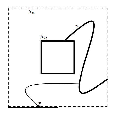
Figure 1: Boundary point connected to $\Lambda_{R}\cup\gamma$ (Lemma 8)

In this figure and the further pictures the free boundary conditions are represented by the dashed lines and the wired boundary conditions are represented by the bold lines.

We use this lemma to obtain the following result.

Lemma 9.

Let us fix $\varepsilon>0$ and $R>0$. Then, for any $n$ large enough, one of the following statements should hold:

1. $$\sum_{x\in\partial^{-}_{b}S_{n}}\phi^{1}_{S_{n},p_{sd},q}[x\longleftrightarrow 0]>R\log n.$$ (28)

2. $$\phi^{0}_{S_{n},p_{sd}-\varepsilon,q}(0\longleftrightarrow\partial\Lambda_{n})<n^{-20}.$$ (29)

For the second case, we can rewrite (29) using the dual model on the dual lattice to get:

$$\phi_{S_{n},(p_{sd}+\delta)^{*},q}^{1^{*}}[A_{n}^{*}]\leq\phi_{S_{n},(p_{sd}+\delta)^{*},q}^{1^{*}}[0\overset{*}{\longleftrightarrow}\partial\Lambda_{n}]\leq n^{-20}.$$ (30)

If the first case holds, then combined with Lemma 5, it gives that for any $R>0$, for $n$ large enough

$$\overline{\varphi}_{p,q,n}(S)>R\log n$$ (31)

for any $S\in S_{n}$ with the properties $\partial^{-}S_{n}\subset S$ and $\partial^{+}S_{n}\cap S=\emptyset$.

The combination of this inequality with Lemma 4 implies the following proposition.

Proposition 10.

For $n$ such that (28) holds and for any $\delta>0$, we have that

$$\phi_{S_{n},(p_{sd}+\delta)^{*},q}^{1^{*}}[A_{n}^{*}]\leq n^{-20}.$$ (32)

The fact that $p_{sd}\geq p_{c}$ for $3<q\leq 4$ is the immediate consequence of (30) and (32) and the following lemma:

Lemma 11 ([Dum13]).

Suppose $p^{\prime}<p_{c}$. Then, for infinitely many $n\in\mathbb{N}$, we have that

$$\phi^{1^{*}}_{S_{n},(p^{\prime})^{*},q}[A_{n}^{*}]>n^{-20}.$$ (33)

The rest of the paper is organised as follows. In Section 5, we show Lemma 4 and Theorem 10. Then in Section 6, we use the parafermionic observable to prove Lemmas 5 and 6. Lemma 7 is proven in Section 7. Then, in Section 8 we focus on Lemma 8. Lemma 9 is the final step to conclude the proof and is shown in Section 9.

5 Proofs of Lemma 4 and Proposition 10.

These proofs use the same strategies as in the case $q\leq 3$.

Proof of Lemma 4.

(see also [DT16, DCT16]). Let us remind that the event complement to $A_{n}$ is equal to $\{\partial^{-}S_{n}\subset\mathcal{S}\}$. Then,

$$\frac{d}{dp}\phi_{S_{n},p,q}^{1}[A_{n}] \geq\frac{c}{1-p}\!\!\sum_{e\in E(S_{n})}\!\phi_{S_{n},p,q}^{1}[e\text{ is pivotal for }A_{n},A_{n}\text{ does not occur}]$$

$$\geq\frac{c}{1-p}\sum_{S:\,\partial^{-}S_{n}\subset S\subset S_{n}}\sum_{(x,y)\in\Delta S}\phi_{S_{n},p,q}^{1}[\partial^{-}S_{n}\underset{S}{\longleftrightarrow}x,\mathcal{S}=S]$$

$$\geq\frac{c}{1-p}\sum_{S:\,\partial^{-}S_{n}\subset S\subset S_{n}}\overline{\varphi}_{p,q,n}(S)\phi_{S_{n},p,q}^{1}[\mathcal{S}=S]$$

$$\geq\frac{c}{1-p}\left(\inf_{S:\,\partial^{-}S_{n}\subset S\subset S_{n}}\overline{\varphi}_{p,q,n}(S)\right)(1-\phi_{S_{n},p,q}^{1}[A_{n}]).$$

∎

Proof of Proposition 10.

This proof uses the same method as for the proof given in Section 3. Fix $p^{\prime}=p_{sd}+\delta$ for some $\delta>0$. By monotonicity, (31) holds for any $p\in[p_{sd},p^{\prime}]$. This together with (24) gives that

$$-d\left(\log(1-\phi_{G,p,q}^{1}[A_{n}])\right)\geq\frac{R}{1-p}\log n\,dp\geq R\log n\,dp.$$

After integrating we obtain that

$$\phi_{G,p_{sd}+\delta,q}^{1}[A_{n}]\geq 1-n^{-R\delta}.$$

Let us choose $R$ large enough to have $R\delta>20$. Then, when $G$ goes to $S_{n}$, we obtain

$$\phi_{S_{n},p_{sd}+\delta,q}^{1}[A_{n}]\geq 1-n^{-20}$$

or, written in the dual model,

$$\phi_{S_{n},(p_{sd}+\delta)^{*},q}^{1^{*}}[A_{n}^{*}]\leq n^{-20}.$$

∎

6 Proof of Lemmas 5 and 6.

Proof of Lemma 6.

This proof uses the same strategy as in Lemma 3, but on $\mathbb{U}_{k}$ instead of $\mathbb{Z}^{2}$. Let us look at a set $S\in\Lambda_{n,k}$ containing $0$ and denote $\overline{S}=\{(-x,y,-z),(x,y,z)\in S\}$ its reflection. We are interested in the connected component containing zero, denoted by $S_{0}$. Let us look at the set $\Lambda_{n,k}^{\prime}=\Lambda_{n,k}\backslash\partial\mathbb{U}_{k}$ and study the sets $S^{\prime}_{0}=\Lambda_{n,k}^{\prime}\cap S_{0}$ and $\overline{S^{\prime}_{0}}=\Lambda_{n,k}^{\prime}\cap\overline{S_{0}}$.

For boundary conditions $(0)$ defined as before we can define the exploration path both for $S^{\prime}_{0}$ and $\overline{S^{\prime}_{0}}$. Its initial and final edges are of the form $e_{a}=\bigl{(}(0,-\tfrac{1}{2},-k)(\tfrac{1}{2},0,-k)\bigr{)}$ and $e_{b}=\bigl{(}(-\tfrac{1}{2},0,k)(0,-\tfrac{1}{2},k)\bigr{)}$. The sets $V,\delta V,\delta_{0},\delta_{1}=\delta_{1}^{+}\cup\delta_{1}^{-}$ and $\delta_{2}$ (resp. $\overline{V},\overline{\delta V},\overline{\delta_{1}}=\overline{\delta_{1}^{+}}\cup\overline{\delta_{1}^{-}}$ and $\overline{\delta_{2}}$) are defined as in previous proof.

Then, (12) enables us to write exactly the same equation as in (17)

$$\bigl{|}\sum_{e\in\delta_{1}\cup\delta_{0}}\eta_{V}(e)\hat{F}_{S^{\prime}_{0}}(e)+\sum_{e\in\overline{\delta_{1}}\cup\delta_{0}}\eta_{\overline{V}}(e)\hat{F}_{\overline{S^{\prime}_{0}}}(e)\bigr{|}\leq\bigl{|}\sum_{e\in\delta_{2}}\eta_{V}(e)\hat{F}_{S_{0}^{\prime}}(e)\bigr{|}+\bigl{|}\sum_{e\in\overline{\delta_{2}}}\eta_{\overline{V}}(e)\hat{F}_{\overline{S_{0}^{\prime}}}(e)\bigr{|}.$$ (34)

As in (18), the right-hand side of (34) is bounded as follows:

$$\bigl{|}\sum_{e\in\delta_{2}}\eta_{V}(e)\hat{F}_{S_{0}^{\prime}}(e)\bigr{|}+\bigl{|}\sum_{e\in\overline{\delta_{2}}}\eta_{\overline{V}}(e)\hat{F}_{\overline{S_{0}^{\prime}}}(e)\bigr{|}\leq 4\!\!\!\sum_{x\in\partial S_{0}}\!\!\phi_{S,p_{sd},q}^{0}(0\longleftrightarrow x).$$ (35)

The left-hand side of (34) can be written as:

$$\bigl{|}\sum_{e\in\delta_{1}\cup\delta_{0}}\eta_{V}(e)\hat{F}_{S^{\prime}_{0}}(e) +\sum_{e\in\overline{\delta_{1}}\cup\delta_{0}}\eta_{\overline{V}}(e)\hat{F}_{\overline{S^{\prime}_{0}}}(e)\bigr{|}=\bigl{|}2(e^{i\hat{\sigma}(4\pi k\frac{3\pi}{2})}-1)$$

$$+\sum_{x\in\partial^{+}_{slit}\cup\partial^{-}_{slit}}\phi^{0}_{S^{\prime}_{0},p_{sd},q}(x\longleftrightarrow 0)(e^{-\pi i\hat{\sigma}}-e^{-i\hat{\sigma}\frac{\pi}{2}}+e^{4k\pi i\hat{\sigma}}(e^{2\pi i\hat{\sigma}}-e^{i\hat{\sigma}\frac{5\pi}{2}}))\bigr{|}$$

$$=\bigl{|}2(e^{i\hat{\sigma}(4\pi k\frac{3\pi}{2})}-1)$$

$$+\sum_{x\in\partial^{+}_{slit}\cup\partial^{-}_{slit}}2\phi^{0}_{S^{\prime}_{0},p_{sd},q}(x\longleftrightarrow 0)(e^{i\hat{\sigma}(2\pi k+\frac{\pi}{2})}-e^{(2k+1)\pi i\hat{\sigma}})\cos((4\pi k+3)\tfrac{\hat{\sigma}}{2})\bigr{|}$$

$$=2\bigl{|}(e^{(2k+1)\pi i\hat{\sigma}}-e^{i\hat{\sigma}(2\pi k+\frac{\pi}{2})})\bigr{|}$$

$$\bigl{|}1+\sum_{m=1}^{4k+1}2\cos(\tfrac{\pi m}{2}\hat{\sigma})-\sum_{x\in\partial^{+}_{slit}\cup\partial^{-}_{slit}}2\phi^{0}_{S^{\prime}_{0},p_{sd},q}(x\longleftrightarrow 0)\cos((4\pi k+3)\tfrac{\hat{\sigma}}{2})\bigr{|}$$

$$\geq 2\bigl{|}(e^{i\hat{\sigma}\tfrac{\pi}{2}}-1)\bigr{|}.$$

The last bound holds if we pick an integer $k$ in such a way that $\cos(\tfrac{\pi m}{2}\hat{\sigma})\geq 0$ for any integer $m\in[0,4k+1]$ and $\cos((4k+3)\tfrac{\pi}{2}\hat{\sigma})\leq 0$. These inequalities give the constraint

$$k\in\biggl{[}\frac{\tfrac{2}{\hat{\sigma}}-3}{2},\frac{\tfrac{2}{\hat{\sigma}}-1}{2}\biggr{]}.$$

The length of this interval is equal to one so such $k$ can always be found.

∎

Proof of Lemma 5.

Look at the exploration path $\gamma$ from $(0,0)$ to $(n,0)$ in the strip $S_{n}$ with $0\backslash 1$ boundary conditions. Take $S$ such that $\partial^{-}S_{n}\subset S\subset S_{n}$ and its reflection $\overline{S}$ from the middle line of the strip. We call $V$ (correspondingly $\overline{V}$) the vertices of $S^{\diamond}$ (correspondingly $\overline{S^{\diamond}}$), and $\delta_{b}^{-},\delta_{t}^{-},\delta_{P^{*}}$ and $\delta_{\overline{P^{*}}}$ the medial edges corresponding to the bottom and top left boundaries of $S_{n}$ and to the paths $P^{*}$ and $\overline{P^{*}}$.

The equation (12) can be written as

$$\bigl{|}\sum_{e\in\delta_{b}^{-}\cup\delta_{t}^{-}}\eta_{V}(e)\hat{F}_{S}(e)+\eta_{\overline{V}}(e)\hat{F}_{\overline{S}}(e)\bigr{|}\leq\bigl{|}\sum_{e\in\delta_{P^{*}}}\eta_{V}(e)\hat{F}_{S}(e)\bigr{|}+\bigl{|}\sum_{e\in\delta_{\overline{P^{*}}}}\eta_{\overline{V}}(e)\hat{F}_{\overline{S}}(e)\bigr{|}.$$ (36)

The right part of the inequality is written as

$$\bigl{|}\sum_{e\in\delta_{P^{*}}}\eta_{V}(e)\hat{F}_{S}(e)\bigr{|}+\bigl{|}\sum_{e\in\delta_{\overline{P^{*}}}}\eta_{\overline{V}}(e)\hat{F}_{\overline{S}}(e)\bigr{|} =2\bigl{|}\sum_{e\in\delta_{P^{*}}}\eta_{V}(e)\hat{F}_{S}(e)\bigr{|}$$

$$\leq 2\sum_{e\in\delta_{P^{*}}}\phi^{0\backslash 1}_{S_{n},p_{sd},q}(e\in\gamma)$$

$$=4\sum_{e\in P^{*}}\phi^{0\backslash 1}_{S_{n},p_{sd},q}(e\longleftrightarrow\partial^{-}S_{n})$$

$$=8\sum_{e\in P^{*}}\phi^{0\backslash 1}_{S_{n},p_{sd},q}(e\longleftrightarrow\partial^{-}_{b}S_{n}).$$

due to the symmetry of $S$ and $\overline{S}$. Also, because of this symmetry, the left-hand side of (36) is bounded by

$$\bigl{|}(e^{i\tfrac{\pi}{2}\hat{\sigma}}-1+e^{-i\tfrac{\pi}{2}\hat{\sigma}}-e^{-i\pi\hat{\sigma}})\!\!\!\sum_{x\in\partial^{-}S_{n}}\!\!\phi^{0\backslash 1}_{S_{n},p_{sd},q}(x\overset{*}{\longleftrightarrow}P^{*})\bigr{|} =\tfrac{\sqrt{q}}{2}\bigl{|}1-e^{-i\tfrac{\pi}{2}\hat{\sigma}}\bigr{|}\!\!\!\sum_{x\in\partial^{-}S_{n}}\!\!\phi^{0\backslash 1}_{S_{n},p_{sd},q}(x\overset{*}{\longleftrightarrow}P^{*})$$

$$=\sqrt{q}\bigl{|}1-e^{-i\tfrac{\pi}{2}\hat{\sigma}}\bigr{|}\!\!\!\sum_{x\in\partial^{-}_{b}S_{n}}\!\!\phi^{0\backslash 1}_{S_{n},p_{sd},q}(x\overset{*}{\longleftrightarrow}P^{*}).$$

The combination of these two bounds finishes the proof. ∎

7 Proof of Lemma 7

To prove this lemma we introduce new definitions and prove one intermediate lemma. For every integer $r$, call $\ell_{r}$ the axis in $\mathbb{U}$ obtained by the rotation of $\ell_{0}\leavevmode\nobreak\ =\leavevmode\nobreak\ \{(0,y,0)\leavevmode\nobreak\ :\leavevmode\nobreak\ y\leavevmode\nobreak\ \geq\leavevmode\nobreak\ 0\}$ by the angle $\tfrac{r\pi}{2}$. Let us denote $\mathrm{sect}_{i,j}$ the part of $\mathbb{U}$ between $\ell_{i}$ and $\ell_{j}$ (in particular $\mathbb{U}_{k}\leavevmode\nobreak\ =\leavevmode\nobreak\ \mathrm{sect}_{-2-4k,4k+2}$).

Let us call the domain $\Omega\subset\mathbb{U}$ symmetric if it is invariant under the reflection with respect to $\ell_{0}$, i.e, if $(x,y,z)\in\Omega$ implies that $(x,-y,-z)\in\Omega$. Let us also call $\Omega$ simple if $0\in\Omega$ and if for any sector $\mathrm{sect}_{i,i+1}$ the domain $\mathrm{sect}_{i,i+1}\backslash\Omega$ is connected.

Lemma 12.

For any $k>0$ and any simple symmetric domain $\Omega$ such that $\Omega\subset\mathrm{sect}_{-k,k}$ the following is true:

$$\phi^{0,0\backslash 1}_{\mathrm{sect}_{-k,k}\backslash\Omega,p_{sd},q}\bigl{(}\ell_{1}\overset{*}{\underset{\mathrm{sect}_{-1,1}}{\longleftrightarrow}}(\partial\Omega\cap\mathrm{sect}_{-1,0})\bigr{)}\geq\frac{1}{2}.$$ (37)

where $0,0\backslash 1$ boundary conditions denote free boundary conditions at infinity, $\ell_{k}$ and $\ell_{-k}$, free boundary conditions on $\mathrm{sect}_{-k,0}\cap\partial\Omega$ and wired boundary conditions on $\mathrm{sect}_{0,k}\cap\partial\Omega$.

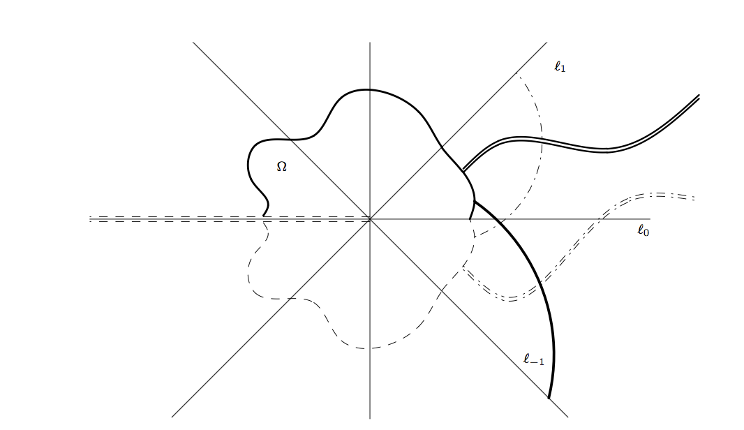
Figure 2: A domain $\Omega$ with corresponding boundary conditions, events $A_{1}$ and $A_{2}$, and $B_{1}$ and $B_{2}$ (doubled lines). Dual paths are represented by dash-dotted lines.

Proof.

The events

$$A_{1}=\{\ell_{1}\overset{*}{\underset{\mathrm{sect}_{-1,1}\backslash\Omega}{\longleftrightarrow}}(\partial\Omega\cap\mathrm{sect}_{-1,0})\}$$

and

$$A_{2}=\{\ell_{-1}{\underset{\mathrm{sect}_{-1,1}\backslash\Omega}{\longleftrightarrow}}(\partial\Omega\cap\mathrm{sect}_{0,1})\}$$

are disjoint. Let us denote $1,0\backslash 1$ the boundary conditions which are wired at infinity, $\ell_{k}$ and $\ell_{-k}$, free at $\mathrm{sect}_{-k,0}\cap\partial\Omega$ and wired at $\mathrm{sect}_{0,k}\cap\partial\Omega$. Then, by duality and by comparison between free and wired boundary conditions (which favour primal paths to appear),

$$\phi^{0,0\backslash 1}_{\mathrm{sect}_{-k,k}\backslash\Omega,p_{sd},q}(A_{1})=\phi^{1,0\backslash 1}_{\mathrm{sect}_{-k,k}\backslash\Omega,p_{sd},q}(A_{2})\geq\phi^{0,0\backslash 1}_{\mathrm{sect}_{-k,k}\backslash\Omega,p_{sd},q}(A_{2}).$$

Let us look at the events

$$B_{1}=\{(\partial\Omega\cap\mathrm{sect}_{0,1}){\underset{\mathrm{sect}_{-1,1}\backslash\Omega}{\longleftrightarrow}}\infty\}$$

and

$$B_{2}=\{(\partial\Omega\cap\mathrm{sect}_{-1,0})\overset{*}{\underset{\mathrm{sect}_{-1,1}\backslash\Omega}{\longleftrightarrow}}\infty\}.$$

The realisations of $A_{2}$ and $B_{1}$ are the only paths blocking the event $A_{1}$ (see Figure 2).

Thus, $A_{1}$, $A_{2}$ and $B_{1}\cap B_{2}$ are disjoint, and moreover, $A_{1}\cup A_{2}\cup(B_{1}\cap B_{2})$ is equal to the full probability space:

$$\phi^{0,0\backslash 1}_{\mathrm{sect}_{-k,k}\backslash\Omega,p_{sd},q}(A_{1})+\phi^{0,0\backslash 1}_{\mathrm{sect}_{-k,k}\backslash\Omega,p_{sd},q}(A_{2})+\phi^{0,0\backslash 1}_{\mathrm{sect}_{-k,k}\backslash\Omega,p_{sd},q}(B_{1}\cap B_{2})=1$$ (38)

Let us bound the probability of $B_{1}\cap B_{2}$. We can compare it to the event

$$\tilde{B}=\{0\overset{*}{\underset{\mathrm{sect}_{-1,1}}{\longleftrightarrow}}\infty,0{\underset{\mathrm{sect}_{-1,1}}{\longleftrightarrow}}\infty$$ and the dual cluster comes before the primal one

$$\text{ on the way from $\ell_{-1}$ to $\ell_{1}$}\}.$$

We can open all edges of $\Omega\cap\mathrm{sect}_{0,1}$ and close all edges of $\Omega\cap\mathrm{sect}_{-1,0}$, this connects the primal cluster from the event $B_{1}$ and the dual cluster from the event $B_{2}$ to zero. Then by finite energy property there exists a positive constant $c$ depending only on $\Omega$, such that

$$c\phi^{0,0\backslash 1}_{\mathrm{sect}_{-k,k}\backslash\Omega,p_{sd},q}(B_{1}\cap B_{2}) \leq\phi^{0}_{\mathrm{sect}_{-k,k},p_{sd},q}(B_{1}\cap B_{2}\cap\{(\Omega\cap\mathrm{sect}_{-1,0})\text{ closed, }(\Omega\cap\mathrm{sect}_{-1,0})\text{ open}\})$$

$$\leq\phi^{0}_{\mathrm{sect}_{-k,k},p_{sd},q}(\tilde{B}).$$

From now on the proof will require that $k\geq 3$, but it can be easily modified for $k\in\{1,2\}$.

Let us look at the probability of the event

$$C=\{0\overset{*}{\underset{\mathrm{sect}_{1,3}}{\longleftrightarrow}}\infty\}$$

conditioned on $\tilde{B}$, and compare it to the event $\tilde{B}$ itself. The existence of the primal cluster from $0$ to infinity in $\mathrm{sect}_{-1,1}$ has less influence on $C$, than a primal cluster from $0$ to infinity in $\mathrm{sect}_{1,-3}$ (closer to $\ell_{1}$, than the dual cluster). The free boundary conditions at $\ell_{k}$ are two $\tfrac{\pi}{2}$-turns closer to the dual cluster from $C$ than the free boundary conditions at $\ell_{-k}$ for the dual cluster of $\tilde{B}$. The comparison between boundary conditions concludes that

$$\phi^{0}_{\mathrm{sect}_{-k,k},p_{sd},q}(C|\tilde{B})\geq\phi^{0}_{\mathrm{sect}_{-k,k},p_{sd},q}(0\overset{*}{\longleftrightarrow}\infty\text{ in }\tilde{B}|0\longleftrightarrow\infty\text{ in }\tilde{B})\geq\phi^{0}_{\mathrm{sect}_{-k,k},p_{sd},q}(\tilde{B}),$$

and, by comparison between boundary conditions,

$$\phi^{0}_{\mathrm{sect}_{-3,1},p_{sd},q}(C\cap\tilde{B})\geq\phi^{0}_{\mathrm{sect}_{-k,k},p_{sd},q}(C\cap\tilde{B})\geq\bigr{(}\phi^{0}_{\mathrm{sect}_{-k,k},p_{sd},q}(\tilde{B})\bigl{)}^{2}.$$

Let us look at the existence of the primal infinite cluster in $C\cap\tilde{B}$ conditioned on the existence of two separated infinite dual clusters (let us call this event $(0\overset{*}{\longleftrightarrow}\infty)^{2}$). The probability of this event will not change if the boundaries $\ell_{-1}$ and $\ell_{3}$ are glued together to obtain $\mathbb{Z}^{2}$. The probability for primal infinite cluster to exist increases if we remove two dual clusters. Thus,

$$\bigr{(}c\phi^{0,0\backslash 1}_{\mathrm{sect}_{-k,k}\backslash\Omega,p_{sd},q}(B_{1}\cap B_{2})\bigl{)}^{2} \leq\phi^{0}_{\mathrm{sect}_{-3,1},p_{sd},q}(C\cap\tilde{B})$$

$$\leq\phi^{0}_{\mathrm{sect}_{-3,1},p_{sd},q}(0{\longleftrightarrow}\infty\text{ in }C\cap\tilde{B}|(0\overset{*}{\longleftrightarrow}\infty)^{2}\text{ in }C\cap\tilde{B})$$

$$\leq\phi^{0}_{\mathbb{Z}^{2},p_{sd},q}(0{\longleftrightarrow}\infty\text{ in }C\cap\tilde{B}|(0\overset{*}{\longleftrightarrow}\infty)^{2}\text{ in }C\cap\tilde{B})$$

$$\leq\phi^{0}_{\mathbb{Z}^{2},p_{sd},q}(0\longleftrightarrow\infty),$$

and the last probability is equal to zero because of Zhang’s argument. Combined with (38), this implies the result.

∎

Proof of Lemma 7.

We are going to prove that, with positive probability, there exists a dual path in $\mathbb{U}_{k}\backslash\Lambda_{n,k}$ disconnecting $0$ from infinity and that this probability does not depend on $n$. This fact implies the statement of the proposition.

Let us look at the event $\{\ell_{-4k-2}\overset{*}{\underset{\mathbb{U}_{k}\backslash\Lambda_{n,k}}{\longleftrightarrow}}\ell_{-4k-1}\}$ not in $\mathbb{U}_{k}=\mathrm{sect}_{-4k-2,4k+2}$, but in a bigger domain $\mathrm{sect}_{-12k-6,4k+2}$. The domain $\Omega=\Lambda_{n,3k+1}\cap\mathrm{sect}_{-12k-6,4k+2}$ is simple and symmetric with respect to the symmetry line $\ell_{-4k-2}$. Putting free boundary conditions on $\ell_{-12k-6}$ and on $\partial\Omega\cap\mathrm{sect}_{-12k-6,-4k-2}$ instead of $\ell_{-4k-2}$ decreases the probability of dual path to appear. Then, by comparison between boundary conditions

$$\phi^{0}_{\mathbb{U}_{k},p_{sd},q}(\ell_{-4k-2} \overset{*}{\underset{\mathbb{U}_{k}\backslash\Lambda_{n,k}}{\longleftrightarrow}}\ell_{-4k-1})$$

$$\geq\phi^{0}_{\mathrm{sect}_{-12k-6,4k+2},p_{sd},q}(\ell_{-4k-2}\!\!\!\!\!\overset{*}{\underset{\mathrm{sect}_{-12k-6,4k+2}\backslash\Omega}{\longleftrightarrow}}\!\!\!\!\!\ell_{-4k-1}|\Omega\cap\mathrm{sect}_{-12k-6,-4k-2}\text{ closed})$$

$$\geq\phi^{0,0\backslash 1}_{\mathrm{sect}_{-12k-6,4k+2}\backslash\Omega,p_{sd},q}(\ell_{-4k-2}\overset{*}{\longleftrightarrow}\ell_{-4k-1})\geq\tfrac{1}{2},$$

where the last bound is a direct consequence of Lemma 12.

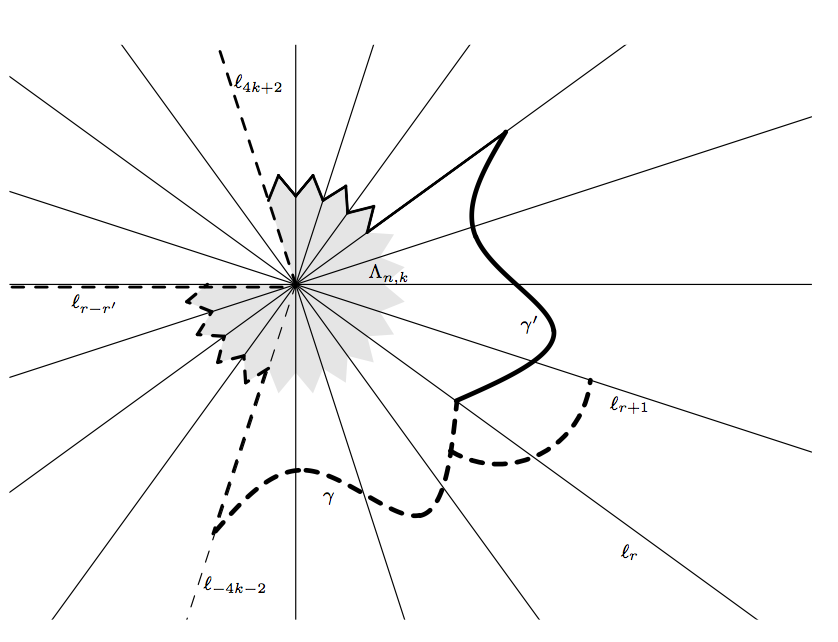
Figure 3: Construction of the dual connection between $\gamma$ and $\ell_{r+1}$

Suppose now that for some integer $r\in[-4k-1,4k+1]$ lines $\ell_{-4k-2}$ and $\ell_{r}$ are already connected in $\mathbb{U}_{k}\backslash\Lambda_{n,k}$ by a dual path $\gamma$ (see Figure 3). Consider $\ell_{r}$ as a symmetry line and reflect $\gamma$ with respect to it (let us call the result $\gamma^{\prime}$). The domain $\Omega^{\prime}$ defined as the area of $\mathrm{sect}_{-4k-2,2r+4k+2}$ bounded by $\gamma\cup\gamma^{\prime}$ is a simple symmetric domain. We are going to work in a sector $\mathrm{sect}_{r-r^{\prime},r+r^{\prime}}$, where $r^{\prime}=4k+2+|r|$. Then $\Omega=(\Lambda_{n,3k+1}\cap\mathrm{sect}_{r-r^{\prime},r+r^{\prime}})\cup\Omega^{\prime}$ is also a simple symmetric domain and, using the same strategy as before, we obtain

$$\phi^{0}_{\mathbb{U}_{k},p_{sd},q}(\ell_{r}\overset{*}{\underset{\mathbb{U}_{k}\backslash\Lambda_{n,k}}{\longleftrightarrow}}\ell_{r+1}\bigm{|}\gamma) \geq\phi^{0}_{\mathrm{sect}_{r-r^{\prime},r+r^{\prime}},p_{sd},q}(\ell_{r}\overset{*}{\underset{\mathrm{sect}_{r-r^{\prime},r+r^{\prime}}\backslash\Omega}{\longleftrightarrow}}\ell_{r+1}\bigm{|}\Omega\cap\mathrm{sect}_{r-r^{\prime},r}\text{ closed})$$

$$\geq\phi^{0,0\backslash 1}_{\mathrm{sect}_{r-r^{\prime},r+r^{\prime}}\backslash\Omega,p_{sd},q}(\ell_{r}\overset{*}{\longleftrightarrow}\ell_{r+1})\geq\tfrac{1}{2}.$$

This implies the result since, by iterative conditioning, we find

$$\phi^{0}_{\mathbb{U}_{k},p_{sd},q}(\ell_{-4k-2}\overset{*}{\underset{U_{k}\backslash\Lambda_{n,k}}{\longleftrightarrow}}\ell_{4k+2})\geq\bigr{(}\tfrac{1}{2}\bigl{)}^{8k+4}.$$

∎

8 Proof of Lemma 8

Proof.

Fix $k$ and $C$ as in Lemma 5 so that:

$$\sum_{x\in\partial\Lambda_{n,k}}\phi^{0}_{\Lambda_{n,k},p_{sd},q}(0\longleftrightarrow x)\geq C.$$

Divide the boundary of $\Lambda_{n,k}$ into $8(2k+1)$ pieces by splitting each side of each boundary layers into two halfs at the midpoint. Then, there exists at least one piece $I_{n,k}$ such that

$$\sum_{x\in I_{n,k}}\phi^{0}_{\Lambda_{n,k},p_{sd},q}(0\longleftrightarrow x)\geq\frac{C}{17k}.$$ (39)

By the finite energy property, there exists a constant $c^{\prime}=c^{\prime}(q,k,\xi)\geq 1$ such that for any $j\in\mathbb{Z}\cap[-k,k]$ and for any $x\in\mathbb{U}_{k}$ the following holds:

$$\frac{1}{c^{\prime}}\geq\frac{\phi^{\xi}_{\mathbb{U}_{k},p,q}[x\longleftrightarrow(0,0,0)]}{\phi^{\xi}_{\mathbb{U}_{k},p,q}[x\longleftrightarrow(0,0,j)]}\geq c^{\prime}.$$ (40)

Combining (39) and (40), we obtain that for some positive constant $c$, independent of $n$,

$$\sum_{x\in I_{n,k}}\phi^{0}_{\Lambda_{n,k},p_{sd},q}[(0,0,j)\longleftrightarrow x]\geq c,$$

where $j$ is the height of $I_{n,k}$. Using a bigger domain with $2k$ layers to centre the $j$-th layer and comparing boundary conditions as in (7), we conclude that

$$\sum_{x\in I_{n}}\phi^{0}_{\Lambda_{n,2k},p_{sd},q}[0\longleftrightarrow x]\geq c,$$

where $I_{n}$ is the projection of $I_{n,k}$ onto the layer of height $0$.

Let us open all edges in a smaller box $\Lambda_{R,2k}$ for some $R\in(0,N)$. Then, we can write the following inequality

$$\sum_{x\in I_{n}}\phi^{0}_{\Lambda_{n,2k},p_{sd},q}[x\longleftrightarrow\Lambda_{R,2k}|\Lambda_{R,2k}\text{ is all open}] \geq\frac{\sum_{x\in I_{n}}\phi^{0}_{\Lambda_{n,2k},p_{sd},q}[0\longleftrightarrow x]}{\phi^{0}_{\Lambda_{n,2k},p_{sd},q}[0\longleftrightarrow\partial\Lambda_{R,2k}]}$$

$$\geq\frac{c}{{\phi^{0}_{\Lambda_{n,2k},p_{sd},q}[0\longleftrightarrow\partial\Lambda_{R,2k}]}}.$$

Also, we can choose any $\gamma$ from $\partial\Lambda_{n}$ to $\partial\Lambda_{R}$, project it on all layers of $\mathbb{U}_{k}$ as $\tilde{\gamma}$ and make $\tilde{\gamma}$ open. Then, we obtain

$$\sum_{x\in I_{n}}\phi^{\xi}_{\Lambda_{n,2k}\backslash(\Lambda_{R,2k}(\tilde{\gamma})),p_{sd},q}[x\longleftrightarrow\Lambda_{R,2k}(\tilde{\gamma})] =\sum_{x\in I_{n}}\phi^{0}_{\Lambda_{2n,k},p_{sd},q}[x\longleftrightarrow\Lambda_{R,2k}|\Lambda_{R,2k}\cup\tilde{\gamma}\text{ are open}]$$

$$\geq\frac{c}{{\phi^{0}_{\Lambda_{n,2k},p_{sd},q}[0\longleftrightarrow\partial\Lambda_{R,2k}]}}.$$

where $\Lambda_{R,2k}(\tilde{\gamma})$ is a union of $\Lambda_{R,2k}$ and $\tilde{\gamma})$, and $\xi$ denotes the boundary conditions wired on $\partial\Lambda_{R,2k}$ and $\tilde{\gamma}$ and free on $\Lambda_{n,2k}$. Notice that $\{x:x\underset{\Lambda_{n,2k}\backslash(\Lambda_{R,2k}\cup\tilde{\gamma})}{\longleftrightarrow}I_{n}\}$ can be projected on $\mathbb{Z}^{2}$ without multiple projections on one point (if not, an open path between two points with the same projection would cross $\tilde{\gamma}$). Thus, we can conclude that

$$\sum_{x\in I_{n}}\phi^{\xi}_{\Lambda_{n}\backslash(\Lambda_{R}\cup\gamma),p_{sd},q}[x\longleftrightarrow\Lambda_{R}\cup\gamma]\geq\frac{c}{{\phi^{0}_{\Lambda_{n,2k},p_{sd},q}[0\longleftrightarrow\partial\Lambda_{R,2k}]}}.$$ (41)

By Lemma 7, for any $\varepsilon>0$, one may choose $R$ large enough that for $n$ large enough

$$\phi^{0}_{\Lambda_{n,2k},p_{sd},q}[0\longleftrightarrow\partial\Lambda_{R,2k}]<\varepsilon.$$

Together with (41), this gives the result.

∎

9 Proof of Lemma 9

Let us call $p_{m,n}=p_{m,n}(C)$ the probability that the box $[-m,m]\times[0,Cm]\in\mathbb{H}$ with wired boundary conditions on $\partial S_{n}$ is crossed from top to bottom, i.e.

$$p_{m,n}=\phi^{1}_{S_{n},p_{sd},q}([-m,m]\times\{0\}\underset{[-m,m]\times[0,Cm]}{\longleftrightarrow}[-m,m]\times\{Cm\}).$$ (42)

Let us fix $C\in\mathbb{N}$ and take $k,m,n\in\mathbb{N}$ such that $2Ckm<n$. For $i\geq 0$, define the domains $L^{b}_{i}$ and $L_{i}^{t}$ as follows:

$$L_{0}^{b}={[-m,m]\times[0,Cm]},$$

$$L_{0}^{t}={[-m,m]\times[n-Cm,n]},$$

$$L_{i}^{b}=L_{i-1}^{b}\cup\bigl{(}L_{i-1}^{b}+(-2m,0)\bigr{)}\cup\bigl{(}{[-m,m]\times[0,Cm]}+(-im,iCm)\bigr{)},$$

$$L_{i}^{t}=L_{i-1}^{t}\cup\bigl{(}L_{i-1}^{t}+(-2m,0)\bigr{)}\cup\bigl{(}{[-m,m]\times[n-Cm,n]}+(-im,-iCm)\bigr{)}.$$

For $i\leq k$, the domains $L_{i}^{t}$ and $L_{i}^{b}$ stay in the strip $S_{n}$ and do not intersect. We are going to study the events

$$A_{m,n,i}^{b}=\bigl{\{}[0,m]\times\{0\}\underset{L_{i}^{b}}{\longleftrightarrow}\{-(i+1)m\}\times\mathbb{Z}\bigr{\}},$$

$$A_{m,n,i}^{t}=\bigl{\{}[0,m]\times\{n\}\underset{L_{i}^{t}}{\longleftrightarrow}\{-(i+1)m\}\times\mathbb{Z}\bigr{\}}.$$

Lemma 13.

For every $k,m,n\in\mathbb{N}$ such that $2Ckm<n$, we have that

$$\phi^{0\backslash 1}_{S_{n},p_{sd},q}(A_{m,n,k}^{b}\cap A_{m,n,k}^{t})\geq(\tfrac{1}{2}-p_{m,n-2Ckm})^{2(k+1)}.$$ (43)

Proof.

We prove the estimate by induction. The event $A_{m,n,0}^{b}$ is rewritten as follows:

$$\bigl{\{}([0,m]\times\{0\}\underset{[-m,m]\times[0,Cm]}{\longleftrightarrow}\{-m\}\times[0,Cm])\bigr{\}}$$

.

Under $0\backslash 1$ boundary conditions, the events

$$\bigl{\{}[0,m]\times\{0\}\underset{[-m,m]\times[0,Cm]}{\longleftrightarrow}([-m,m]\times\{Cm\})\cup(\{-m\}\times[0,Cm]\bigr{\}}$$

and

$$\bigl{\{}[-m,0]\times\{0\}\overset{*}{\underset{[-m,m]\times[0,Cm]}{\longleftrightarrow}}([-m,m]\times\{Cm\})\cup(\{m\}\times[0,Cm])\bigr{\}}$$

have the same probability. Since by duality and symmetry at least one of them should occur in any configuration, we find that

$$\phi^{0\backslash 1}_{S_{n},p_{sd},q}([0,m]\times\{0\}\underset{[-m,m]\times[0,Cm]}{\longleftrightarrow}([-m,m]\times\{Cm\})\cup(\{-m\}\times[0,Cm]))\geq\frac{1}{2}.$$

Adding wired boundary conditions increase the probability to have a vertical crossing of the box so

$$\phi^{0\backslash 1}_{S_{n},p_{sd},q}([-m,m]\times\{0\}\underset{[-m,m]\times[0,Cm]}{\longleftrightarrow}[-m,m]\times\{Cm\})\leq p_{m,n}$$

which implies that

$$\phi^{0\backslash 1}_{S_{n},p_{sd},q}(A^{b}_{m,n,0})=\phi^{0\backslash 1}_{S_{n},p_{sd},q}([0,m]\times\{0\}\underset{[-m,m]\times[0,Cm]}{\longleftrightarrow}\{-m\}\times[0,Cm])\geq\frac{1}{2}-p_{m,n}.$$

The same estimation is true also for $A^{t}_{m,n,0}$. Then, the FKG inequality gives that

$$\phi^{0\backslash 1}_{S_{n},p_{sd},q}(A^{b}_{m,n,0}\cap A^{t}_{m,n,0})\geq\bigl{(}\frac{1}{2}-p_{m,n}\bigr{)}^{2}.$$

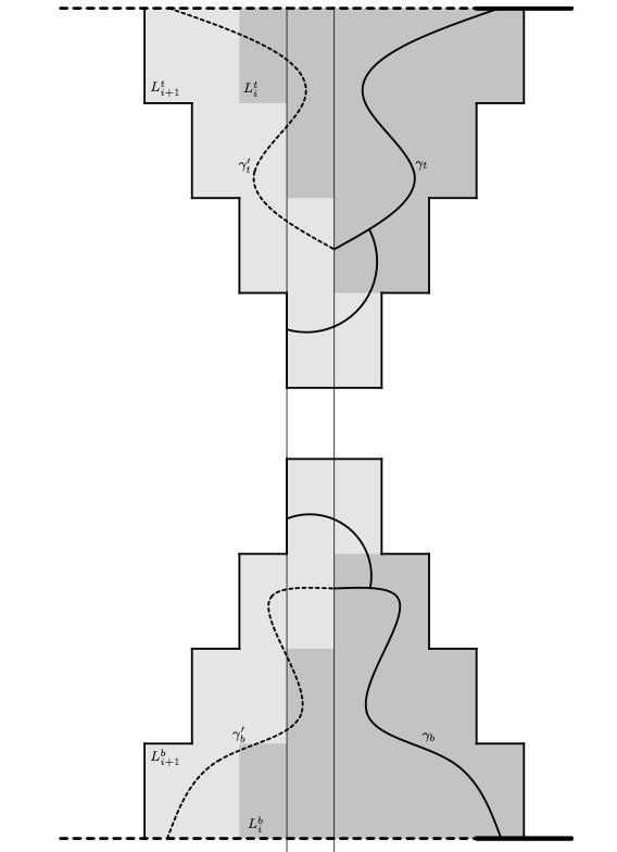
Figure 4: Events $A^{b}_{m,n,i+1}$ and $A^{t}_{m,n,i+1}$ with corresponding boundary conditions.

Suppose now that for some $i$,

$$\phi^{0\backslash 1}_{S_{n},p_{sd},q}(A^{b}_{m,n,i}\cap A^{t}_{m,n,i})\geq(\tfrac{1}{2}-p_{m,n-2Cim})^{2(i+1)}.$$

Let us first notice that $p_{m,n}$ decreases with respect to the second argument because of the Domain Markov property (narrowing the strip by adding wired boundary conditions increases the probability to have a crossing in a box inside it). Thus, we can write that

$$\phi^{0\backslash 1}_{S_{n},p_{sd},q}(A^{b}_{m,n,i}\cap A^{t}_{m,n,i})\geq(\tfrac{1}{2}-p_{m,n-2C(i+1)m})^{2(i+1)}.$$ (44)

Let us look at the event $A^{b}_{m,n,i+1}$ conditioned on the events $A^{b}_{m,n,i}$ and $A^{t}_{m,n,i}$ (see Figure 4). Let $\gamma_{b}$ be the uppermost path from $[0,m]\times\{0\}$ to $\{-(i+1)m\}\times\mathbb{Z}$ satisfying $A^{b}_{m,n,i}$ and $\gamma_{t}$ be the lowermost path from $[0,m]\times\{n\}$ to $\{-(i+1)m\}\times\mathbb{Z}$ satisfying $A^{t}_{m,n,i}$. Let $\gamma_{b}^{\prime}$ and $\gamma_{t}^{\prime}$ be the reflections of $\gamma_{b}$ and $\gamma_{t}$ with respect to the line $\{-(i+1)m\}\times\mathbb{Z}$. Note that $\{-(i+1)m\}\times\mathbb{Z}$ is an axis of symmetry for $L^{b}_{i+1}$ and $L^{t}_{i+1}$.

Set the boundary conditions to be free on $\gamma^{\prime}_{b}$ and $\gamma^{\prime}_{t}$ (this can only decrease the probability of $A^{b}_{m,n,i+1}$). Then, by the same reasons as for $A_{m,n,0}$, the probability to have an open path from $([0,n]\times\{0\})\cup\gamma$ to the top or to the left boundary of $L^{b}_{i+1}$ is bigger than $\tfrac{1}{2}$.

The probability for this path to hit the top part of $\partial L^{b}_{i+1}$ (i.e. $[-(i+2)m,-im]\times\{(i+2)Cm\}$) is smaller than the probability for $[-m,m]\times[0,Cm]+(-(i+1)m,(i+1)Cm)$ to be crossed from top to bottom, which can be bounded above using the comparison between boundary conditions and the Domain Markov property. If we restrict our strip to $\mathbb{Z}\times[(i+1)Cm,n-(i+1)Cm]$ (all the paths will be left outside the strip) and put wired boundary conditions on its boundary, the probability $[-(i+2)m,-im]\times[(i+1)Cm,(i+2)Cm]$ to have a vertical crossing is equal to $p_{m,n-2C(i+1)m}$. The initial domain is bigger and has smaller boundary conditions, so the probability of this event is smaller in this context. This leads to

$$\phi^{0\backslash 1}_{S_{n},p_{sd},q}(A^{b}_{m,n,i+1}|A^{b}_{m,n,i}\cap A^{t}_{m,n,i})\geq\tfrac{1}{2}-p_{m,n-2C(i+1)m},$$

and the same bound holds for $A^{t}_{m,n,i+1}$. By FKG inequality, we deduce that

$$\phi^{0\backslash 1}_{S_{n},p_{sd},q}(A^{b}_{m,n,i+1}\cap A^{t}_{m,n,(i+1)}|A^{b}_{m,n,i}\cap A^{t}_{m,n,i})\geq\bigl{(}\tfrac{1}{2}-p_{m,n-2C(i+1)m}\bigr{)}^{2}.$$

Combining it with $\eqref{hugoadd}$, we deduce that

$$\phi^{0\backslash 1}_{S_{n},p_{sd},q}(A^{b}_{m,n,i+1}\cap A^{t}_{m,n,(i+1)})\geq\bigl{(}\tfrac{1}{2}-p_{m,n-2C(i+1)m}\bigr{)}^{2(i+2)}.$$

Letting $i$ be equal to $k$ gives the result. ∎

Corollary 14.

Let us fix $C\geq 4$ and $m,n\in\mathbb{N}$ such that

$$n\geq 9C^{2}m.$$ (45)

Let us call $A^{b}_{C}$ the event that $[0,m]\times\{0\}$ is connected either to $\{-4Cm-m\}\times[0,8Cm]$ or to $[-4Cm-m,m]\times\{8Cm\}$ in $[-4Cm-m,4Cm-m]\times[0,8Cm]\cap L^{b}_{4C}$.

Then,

$$\phi^{0\backslash 1}_{S_{n},p_{sd},q}(A^{b}_{C})\geq(\tfrac{1}{2}-p_{m,C^{2}m})^{2(4C+1)}.$$ (46)

Proof.

The result follows directly from the fact that $p_{m,n}$ is decreasing in the second variable and from the previous lemma applied to $A_{m,n,4C}$. The built path either ends at $\{-4Cm-m\}\times[0,8Cm]$ or leaves the box from the top boundary. ∎

Lemma 15.

For any choice of $C\geq 4$ and $M>0$, we have that

$$\sum_{x\in[-(4C+1)m,-m]\times\{0\}}\phi^{0\backslash 1}_{S_{n},p_{sd},q}(x\longleftrightarrow 0)\geq M(\tfrac{1}{2}-p_{m,C^{2}m})^{2(4C+1)}$$ (47)

for $m$ large enough and $n\in\mathbb{N}$ such that (45) holds.

Proof.

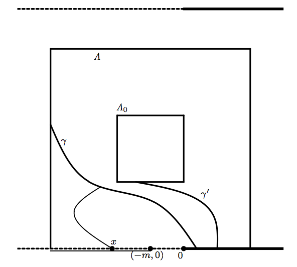
Figure 5: Connection of a point $x$ to $\gamma$ is more probable than its connection to $\gamma^{\prime}\cup\mathit{\Lambda}_{0}$

Let us choose $R$ according to Lemma 8, $m\geq R$ and $n\geq 9C^{2}m$ and look at the square box $\mathit{\Lambda}=\Lambda_{4Cm}+(-m,4Cm)$ with the smaller box $\mathit{\Lambda}^{0}=\Lambda_{R}+(-m,4Cm)$ inside.

Then, conditioned on $A^{b}_{C}$, let $\gamma$ be the uppermost realisation of the path going from $[0,m]\times\{0\}$ to the left or upper parts of $\partial\mathit{\Lambda}$ in the domain described in Corollary 14 (see Figure 5). Note that $\gamma$ lies in the annulus $\mathit{\Lambda}\backslash\mathit{\Lambda}^{0}$. Let us choose $\gamma^{\prime}$ connecting $\partial\mathit{\Lambda}$ and $\mathit{\Lambda}^{0}$ and going to the right from $\gamma$. Then, by Lemma 8,

$$\sum_{x\in[-(4C+1)m,-m]\times\{0\}}\!\!\!\!\!\!\!\!\!\!\!\phi^{0\backslash 1}_{S_{n},p_{sd},q}(x\longleftrightarrow\gamma)\geq\!\!\!\!\!\!\!\!\!\!\!\sum_{x\in[-(4C+1)m,-m]\times\{0\}}\!\!\!\!\!\!\!\!\!\!\!\phi^{0}_{\mathit{\Lambda},p_{sd},q}(x\longleftrightarrow\mathit{\Lambda}^{0}\cup\gamma\,|\,\mathit{\Lambda}^{0}\cup\gamma\text{ are open})\geq M.$$

Increasing the domain to $S_{n}$ and putting wired boundary conditions on $\partial^{+}S_{n}$ only increases the probabilities in the sum. Together with Corollary 14, this gives the result. ∎

Let us now fix any $\varepsilon>0$ and define $\rho=\rho(\varepsilon)>1$ and $C=C(\rho)>4$ large enough that

$$(C+1)\leq\rho^{C}$$ (48)

and

$$C\geq 2\left(\tfrac{\rho}{\rho-1}\right)^{2}$$ (49)

and look at the set

$$K_{n}=\{k\in\mathbb{N},k\leq\log_{\rho}\tfrac{n}{9C^{2}},p_{\rho^{k}(1-\rho),n}\leq\tfrac{1}{4}\}.$$

We will prove that we are either in Case 1 or in Case 2 of Lemma 9 depending on whether $|K_{n}|$ is large or not.

Lemma 16.

Fix $R>0$. For any choice of $\rho>1$ and for any $n$ large enough, if $|K_{n}|\geq\tfrac{1}{2}\log_{\rho}\tfrac{n}{9C^{2}}$, then

$$\sum_{x\in[-n,0)}\phi^{0\backslash 1}_{S_{n},p_{sd},q}((x,0)\longleftrightarrow 0)\geq R\log n.$$

Proof.

Inequality (48) together with the condition $|K_{n}|\geq\tfrac{1}{2}\log_{\rho}\tfrac{n}{9C^{2}}$ allows to pick $\tfrac{1}{10C}\log_{\rho}\tfrac{n}{9C^{2}}$ indices $k\in K_{n}$ such that the intervals

$$I_{k}=[-(4C+1)\rho^{k},-\rho^{k}]$$

are disjoint. Let us choose $M=20RC4^{2(4C+1)}$ and apply Lemma 15 to each $I_{k}$. Then, we obtain

$$\sum_{x\in[-n,0)}\phi^{0\backslash 1}_{\mathbb{H},p_{sd},q}((x,0)\longleftrightarrow 0) \geq\sum_{k}\sum_{x\in I_{k}}\phi^{0\backslash 1}_{\mathbb{H},p_{sd},q}((x,0)\longleftrightarrow 0)$$

$$\geq\frac{M}{10C4^{2(4C+1)}}\log_{\rho}\tfrac{n}{9C^{2}}\geq R\log n.$$

Notice that $R$ is positive and can be picked arbitrary large for $n$ big enough. ∎

Lemma 17.

Take $n$ large enough and suppose that $|K_{n}|\leq\tfrac{1}{2}\log_{\rho}\tfrac{n}{C}$, then

$$\phi^{0}_{\mathbb{H},p_{sd}-\varepsilon,q}(0\longleftrightarrow\partial\Lambda_{n})<n^{-20}.$$

To prove this theorem we need an additional result. Let us define the Hamming distancebetween two configurations $\omega$ and $\omega^{\prime}$ by

$$H(\omega,\omega^{\prime})\coloneqq\sum_{e\in E(\Omega)}|\omega(e)-\omega^{\prime}(e)|,$$

and the Hamming distance between an event $A$ and a configuration $\omega$ ] by

$$H_{A}(\omega)\coloneqq\inf_{\omega^{\prime}\in A}H(\omega,\omega^{\prime}).$$

Then, we can write an inequality similar to (8) in the terms of the expected Hamming distance [Gri06]:

$$\frac{d}{dp}\log\phi^{\xi}_{G,p,q}(A)\geq\frac{1}{p(1-p)}\phi^{\xi}_{G,p,q}(H_{A}).$$ (50)

We now turn to the proof.

Proof.

Let us study the probability of the following event:

$$\mathcal{A}_{k}=\left\{[-2\rho^{k+1},-2\rho^{k}]\times\{0\}\longleftrightarrow[2\rho^{k},2\rho^{k+1}]\times\{0\}\text{ in }A_{n}\right\}$$ (51)

where $A_{k}$ is the half-annulus

$$A_{k}=[-2\rho^{k+1},2\rho^{k+1}]\times[0,C\rho^{k}(\rho-1)]\backslash[-2\rho^{k},2\rho^{k}]\times[0,C\rho^{k-1}(\rho-1)]$$

(see Figure 6).

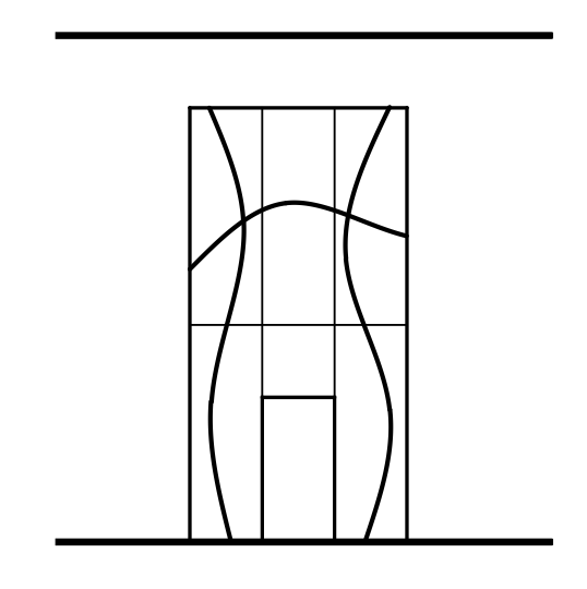
Figure 6: Realisation of $\mathcal{A}_{k}$

The rectangles $[-2\rho^{k+1},-2\rho^{k}]\times[0,C\rho^{k}(\rho-1)]$ and $[2\rho^{k},2\rho^{k+1}]\times[0,C\rho^{k}(\rho-1)]$ are crossed in the vertical direction with probability $p_{\rho^{k}(1-\rho)}$ each. Inequality (49) implies that $A_{k}$ contains a square of size $4\rho^{k+1}$ that is crossed with probability bigger than $\tfrac{1}{2}$. Altogether, this gives a bound $\phi^{1}_{S_{n},p_{sd},q}(\mathcal{A}_{k})\geq\tfrac{1}{2}p^{2}_{\rho^{k}(1-\rho)}$. The assumption on the size of $K_{n}$ implies that $\phi^{1}_{S_{n},p_{sd},q}(\mathcal{A}_{k})\geq\tfrac{1}{32}$ for at least $\tfrac{1}{2C}\log_{\rho}\tfrac{n}{9C^{2}}$ values of $k$. Notice also that for all these indices, $A_{k}$ lies in $\Lambda_{n}$ and that the $A_{k}$ are disjoint.

We study this probability for $p=p_{sd}$ so $\mathcal{A}_{k}$ implies the existence of dual-open circuit in $\mathbb{H}^{*}$ disconnecting $0$ from $\partial\Lambda_{n}$. The expected number of such disjoint circuits is bigger than $\tfrac{1}{64}\log_{\rho}\tfrac{n}{C}$, since the $A_{k}$ are disjoint. This number bounds from below the expectation of the Hamming distance of the event that $0$ is connected to $\partial\Lambda_{n}$ in the dual lattice:

$$\phi^{1^{*}}_{\mathbb{H},(p_{sd})^{*}\!\!,q}(H_{0\overset{*}{\longleftrightarrow}\partial\Lambda_{n}})=\phi^{0}_{\mathbb{H},p_{sd},q}(H_{0\longleftrightarrow\partial\Lambda_{n}})\geq\tfrac{1}{64}\log_{\rho}\tfrac{n}{C}.$$

Here, we changed to the primal lattice with free boundary conditions using the self-duality of the model for $p_{sd}$. We apply (50) to obtain

$$\frac{d}{dp}\log\phi^{0}_{\mathbb{H},p_{sd},q}[0\longleftrightarrow\partial\Lambda_{n}]>\frac{1}{64}\log_{\rho}\frac{n}{C}.$$

By monotonicity, this inequality extends to every $p\in[p_{sd}-\varepsilon^{\prime},p_{sd}]$ for $\varepsilon>0$. Integrating the previous inequality gives:

$$\int_{p_{sd}-\varepsilon}^{p_{sd}}\frac{d}{dp}\log\phi^{0}_{\mathbb{H},p,q}[0\longleftrightarrow\partial\Lambda_{n}]\geq\frac{\varepsilon}{64}\log_{\rho}\frac{n}{C},$$

or, put differently,

$$\phi^{0}_{\mathbb{H},p_{sd}-\varepsilon,q}[0\longleftrightarrow\partial\Lambda_{n}]\leq\left(\tfrac{C}{n}\right)^{\frac{\varepsilon}{64\log\rho}}.$$

The value of $\rho$ was chosen close enough to $1$ that

$$\frac{\varepsilon}{64\log\rho}>20.$$

This concludes the proof. ∎

References

- [BDC12] Vincent Beffara and Hugo Duminil-Copin. The self-dual point of the two-dimensional random-cluster model is critical for . Probability Theory and Related Fields, 153(3):511–542, Aug 2012.
- [BDS15] V. Beffara, H. Duminil-Copin, and S. Smirnov. On the critical parameters of the random-cluster model on isoradial graphs. Journal of Physics A Mathematical General, 48:484003, December 2015.
- [DCST17] Hugo Duminil-Copin, Vladas Sidoravicius, and Vincent Tassion. Continuity of the phase transition for planar random-cluster and potts models with . Communications in Mathematical Physics, 349(1):47–107, Jan 2017.
- [DCT16] Hugo Duminil-Copin and Vincent Tassion. A new proof of the sharpness of the phase transition for bernoulli percolation and the ising model. Communications in Mathematical Physics, 343(2):725–745, Apr 2016.
- [DGPS17] H. Duminil-Copin, A. Glazman, R. Peled, and Y. Spinka. Macroscopic loops in the loop model at Nienhuis’ critical point. ArXiv e-prints, July 2017.
- [DM14] H. Duminil-Copin and I. Manolescu. The phase transitions of the planar random-cluster and Potts models with q larger than 1 are sharp. ArXiv e-prints, September 2014.
- [DRT17] H. Duminil-Copin, A. Raoufi, and V. Tassion. Sharp phase transition for the random-cluster and potts models via decision trees. ArXiv e-prints, May 2017.
- [DS10] H. Duminil-Copin and S. Smirnov. The connective constant of the honeycomb lattice equals . ArXiv e-prints, July 2010.
- [DT16] H. Duminil-Copin and V. Tassion. A new proof of the sharpness of the phase transition for bernoulli percolation on . L’Enseignement mathématique, 62:199–206, 2016.
- [Dum13] H. Duminil-Copin. Parafermionic observables and their applications to planar statistical physics models, volume 25. Ensaios Matematicos, Brazilian Mathematical Society, 2013.
- [ES88] Robert G. Edwards and Alan D. Sokal. Generalization of the Fortuin-Kasteleyn-Swendsen-Wang representation and Monte Carlo algorithm. Phys. Rev. D, 38:2009–2012, Sep 1988.
- [FK72] C.M. Fortuin and P.W. Kasteleyn. On the random-cluster model: I. Introduction and relation to other models. Physica, 57(4):536 – 564, 1972.
- [FKG71] C. M. Fortuin, P. W. Kasteleyn, and J. Ginibre. Correlation inequalities on some partially ordered sets. Comm. Math. Phys., 22(2):89–103, 1971.
- [For72a] C.M. Fortuin. On the random-cluster model: II. The percolation model. Physica, 58(3):393 – 418, 1972.
- [For72b] C.M. Fortuin. On the random-cluster model: III. The simple random-cluster model. Physica, 59(4):545 – 570, 1972.
- [Gla14] A. Glazman. Connective constant for a weighted self-avoiding walk on . ArXiv e-prints, February 2014.
- [Gri99] G. Grimmett. Percolation. Springer Verlag, 1999.
- [Gri06] G. Grimmett. The Random-Cluster model. Springer-Verlag, 2006.
- [Lis17] M. Lis. Circle patterns and critical Ising models. ArXiv e-prints, December 2017.
- [Smi10] S. Smirnov. Conformal invariance in random cluster models. I. Holomorphic fermions in the Ising model. Ann. of Math., 172:1435–1467, 2010.