Gravitational acceleration in a class of geometric sigma models

Abstract

In this work, I examine spherically symmetric solutions in geometric sigma models with four scalar fields. This class of models turns out to be a subclass of the wider class of scalar-vector-tensor theories of gravity. The purpose of the present study is to examine how the additional four degrees of freedom modify Newtonian gravitational acceleration. I have restricted my considerations to pointlike sources in de Sitter background. The resulting gravitational acceleration has the form of a power series, with four major terms standing out. The first and the second are the familiar Newtonian and MOND terms, which dominate at short distances. The third term is dominant at large distances. It is the $\Lambda$CDM term responsible for the accelerated expansion of the Universe. Finally, the fourth term provides an extra repulsive acceleration that grows exponentially fast with distance. This term becomes significant only at extremely large distances that go beyond the observable Universe. As for the time dependence of the calculated gravitational acceleration, it turns out to have nontrivial, oscillatory character.

I Introduction

In the existing literature, the subjects of the early and the late time cosmologies are almost exclusively addressed separately. Indeed, the present epoch is commonly described by the standard cosmological model ($\Lambda$CDM), which makes no predictions concerning the early Universe. In particular, it lacks inflation, which is believed to correctly describe the early Universe. On the other hand, the inflationary models that one encounters in scientific literature are hardly ever checked for their influence on the small scale problems of the present epoch. For example, the known problem of flat galactic curves 1 ; 2 ; 3 ; 4 ; 5 ; 6 ; 7 ; 8 may well be connected to the modification of gravity brought by the inflationary models. Thus, before making an ad hoc modification of gravity, one is advised to first examine the modifications found in the existing cosmological models.

In what follows, I shall examine a class of geometric sigma models with four scalar fields. These models have first been proposed in Ref. 16 in the context of fermionic excitations of flat geometry. In Ref. 18 they are used for the construction of various inflationary and bouncing cosmologies. It has been shown that the resulting cosmologies have everywhere regular and stable backgrounds irrespective of their specific types. In particular, small metric perturbations are demonstrated to regularly pass through the bounce. By inspecting the particle spectrum of these models, they are shown to belong to a wider class of scalar-vector-tensor theories of gravity. My primary motivation is to find out if these theories can be as successful in explaining the late time behavior of the Universe as they are successful in explaining the early Universe. In particular, I want to calculate the modified gravitational acceleration and see if it can fit the observation. To this end, I shall consider a pointlike source, and calculate spherically symmetric metric far from it.

The results of the paper are summarized as follows. The needed spherically symmetric solution is found for the whole class of considered geometric sigma models. The solution is obtained in a weak field approximation, and in the form of a power series. As it turns out, the corresponding coefficients are subject to a set of well defined recurrent relations. These recurrent relations are solved in de Sitter background, which is commonly assumed to characterize the present epoch. This way, the obtained late time behavior of the gravitational acceleration is shown to hold true for all the models with $\Lambda$CDM limit. The integration constants are determined from the requirement that gravitational acceleration reproduces Milgrom’s modified Newtonian dynamics (MOND) at short distances, and the familiar $\Lambda$CDM behavior at large distances. The resulting expression is a sum of four major contributions, which one by one, become dominant as the distance from the gravitational source grows. At short distances, the dominant contribution comes from the Newtonian term. Then, at longer distances, the dominant role is taken by the familiar MOND term. At even larger distances, the leading role is carried by the $\Lambda$CDM term which is responsible for the accelerated expansion of the Universe. Finally, the fourth term provides an extra repulsive acceleration that grows exponentially fast with distance. This term becomes significant only at extremely large distances that go beyond the observable Universe. As such, it can be neglected in practically all astronomical measurements. As the final achievement of this work, let me mention time dependence of the gravitational acceleration. It is shown that gravitational acceleration of the pointlike source has oscillatory dependence on cosmic time. In particular, the gravitational acceleration that is attractive at the present time could have been repulsive at earlier times.

The results obtained in this paper should be confronted with results of similar considerations in literature. Plenty of modified gravity theories considered in literature predict corrections to the Newtonian gravitational force that can explain the unexpected astronomical data. For example, the authors of Refs. 18x and 18y consider a class of $f(R)$ theories of gravity, and succeed in recovering the observed behavior of many spiral and elliptical galaxies. In particular, the $f(R)\propto R^{3/2}$ theory is shown to lead to the familiar MOND behavior 18y . However, all these results are obtained by considering a static metric in a flat background. As a consequence, the obtained gravitational force is necessarily time independent. This should be confronted with the present paper, where the considered pointlike source is placed in a nontrivial cosmic background, and the metric ansatz is not static. As a consequence, the obtained gravitational force has a nontrivial time dependence.

The layout of the paper is as follows. In Sec. II, a precise definition of the class of models to be considered is given. The very construction of geometric sigma models is only briefly recapitulated. In Sec. III, spherically symmetric ansatz is applied to field equations. The solution is obtained in a weak field approximation, and in the form of a power series. The resulting expression holds true for any choice of the scale factor $a$, and the potential $W$. In Sec. IV, a particularly simple choice of $a$ and $W$ has been made. Specifically, the background metric that defines the model is chosen to be of de Sitter type. This choice is in agreement with the common belief that whatever type of the Universe is considered, its late time behavior should be that of the $\Lambda$CDM model. In Sec. V, the nonrelativistic formula for gravitational acceleration is derived. The result is compared with MOND and $\Lambda$CDM predictions. Sec. VI is devoted to concluding remarks.

My conventions are as follows. Indexes $\mu$, $\nu$, … and $i$, $j$, … from the middle of alphabet take values $0,1,2,3$. Indexes $\alpha$, $\beta$, … and $a$, $b$, … from the beginning of alphabet take values $1,2,3$. Spacetime coordinates are denoted by $x^{\mu}$, ordinary differentiation uses comma ($X_{,\,\mu}\equiv\partial_{\mu}X$), and covariant differentiation uses semicolon ($X_{;\,\mu}\equiv\nabla_{\mu}X$). Repeated indexes denote summation: $X_{\alpha\alpha}\equiv X_{11}+X_{22}+X_{33}$. Signature of the $4$-metric $g_{\mu\nu}$ is $(-,+,+,+)$, and curvature tensor is defined as $R^{\mu}{}_{\nu\lambda\rho}\equiv\partial_{\lambda}\Gamma^{\mu}{}_{\nu\rho}-\partial_{\rho}\Gamma^{\mu}{}_{\nu\lambda}+\Gamma^{\mu}{}_{\sigma\lambda}\Gamma^{\sigma}{}_{\nu\rho}-\Gamma^{\mu}{}_{\sigma\rho}\Gamma^{\sigma}{}_{\nu\lambda}$. Throughout the paper, the natural units $c=\hbar=1$ are used.

II Geometric sigma models

The model considered in this paper belongs to the class of geometric sigma models, originally defined in Ref. 16 . The main feature of every geometric sigma model is that it is defined by associating action functional with a fixed, freely chosen metric $g_{\mu\nu}^{(o)}(x)$. The action has the form

$$I_{g}=\frac{1}{2\kappa}\int d^{4}x\sqrt{-g}\left[R-F_{ij}(\phi)\phi^{i}_{,\mu}\phi^{j,\mu}-V(\phi)\right],$$ (1)

where $F_{ij}(\phi)$ and $V(\phi)$ are target metric and potential of four scalar fields $\phi^{i}(x)$. The constant $\kappa\equiv 8\pi G$ stands for the gravitational coupling constant. The target metric $F_{ij}(\phi)$ is constructed by replacing $x^{i}$ with $\phi^{i}$ in the expression

$$F_{ij}(x)\equiv R_{ij}^{(o)}(x)-\frac{1}{2}V(x)g_{ij}^{(o)}(x)\,,$$ (2)

where $R_{\mu\nu}^{(o)}(x)$ is Ricci tensor for the metric $g_{\mu\nu}^{(o)}(x)$. The same replacement in an arbitrary function $V(x)$ defines the potential $V(\phi)$. This construction guarantees that

$$\phi^{i}=x^{i}\,,\quad g_{\mu\nu}=g_{\mu\nu}^{(o)}$$ (3)

is a solution of the field equations defined by Eq. (1). In what follows, the solution Eq. (3) will be referred to as vacuum. It is seen that physics of small perturbations of this vacuum allows the gauge condition

$$\phi^{i}(x)=x^{i}\,.$$ (4)

Gauge fixed field equations employ the metric alone, and read

$$R_{\mu\nu}=R_{\mu\nu}^{(o)}(x)+\frac{1}{2}V(x)\left(g_{\mu\nu}-g_{\mu\nu}^{(o)}\right).$$ (5)

In what follows, I shall be interested in how a pointlike source deforms the surrounding empty background. Thus, the needed field equations will be the matter free equations (5).

The cosmological background I choose to work with is the background metric

$$ds^{2}=-dt^{2}+a^{2}(t)\left(dx^{2}+dy^{2}+dz^{2}\right).$$ (6)

It defines the vacuum metric $g_{\mu\nu}^{(o)}$. The model itself is defined by determining $V(x)$ and $F_{ij}(x)$. For the vacuum metric Eq. (6), one finds

$$F_{00}=W-2\dot{H}\,,\quad F_{0b}=0\,,\quad F_{ab}=-a^{2}\,W\delta_{ab}\,,$$ (7)

where $H\equiv\dot{a}/a$ is the Hubble parameter, and $W$ is defined by

$$V\equiv 2\left(W+\dot{H}+3H^{2}\right).$$ (8)

The “dot” denotes time derivative. The target metric $F_{ij}(\phi)$ and the potential $V(\phi)$ are obtained by the substitution $x^{i}\to\phi^{i}$ in $F_{ij}(x)$ and $V(x)$. For the time being, the scale factor $a(t)$, and the potential $W(t)$ are kept unspecified.

In what follows, the most general case $W\neq 0$ will be considered. This is motivated by the failure of Ref. 18a , where $W=0$ case was studied, to provide an acceptable explanation of flat galactic curves. The $W\neq 0$ geometric sigma models have extensively been studied in Ref. 18 . There, they were used for the construction of various inflationary and bouncing cosmologies. It has been shown that the resulting cosmologies have everywhere regular and stable backgrounds irrespective of their specific types. The necessary conditions for proving regularity and stability have been shown to read

$$W<0\,,\quad F_{00}<0\,.$$ (9)

If, in addition, one makes the choice

$$W=-\frac{\omega^{2}}{a^{2}}\,,$$ (10)

where $\omega$ is a constant with the dimension of mass, the regularity and stability are guaranteed. This choice of $W$ is not unique, but is certainly sufficient to make the theory everywhere well defined. By inspecting the particle spectrum, these models have been shown to belong to a wider class of scalar-vector-tensor theories of gravity. All their modes are massive. In particular, the graviton mass is

$$m_{g}=\sqrt{-2W}\,.$$ (11)

The good thing about this is that, in most physically relevant situations, the value of $m_{g}$ stays below its experimental bound. This makes the described class of geometric sigma models physically liable. My primary motivation in this paper is to find out if these theories can be as successful in explaining the small scale problems of the present epoch as they are successful in explaining the early Universe. In particular, I want to calculate the gravitational acceleration of a pointlike source in a nontrivial cosmic background.

III Field equations

In what follows, matter fields are assumed to be localized in a point, which I choose to be $\vec{x}=0$. Then, the field equations in the region $\vec{x}\neq 0$ reduce to those obtained from the geometric action Eq. (1). In the gauge Eq. (4), the field equations reduce to Eq. (5), and possess the vacuum solution $g_{\mu\nu}=g_{\mu\nu}^{(o)}$. What I am interested in are spherically symmetric deviations from this vacuum, caused by the presence of a massive particle in $\vec{x}=0$. It is important to emphasize that the gauge Eq. (4) leaves us with no residual gauge symmetry. Thus, no further gauge fixings are possible.

The most general spherically symmetric metric in the gauge Eq. (4) has the form

$$g_{00}=\mu\,,\quad g_{0\alpha}=\nu\frac{x_{\alpha}}{r}\,,\quad g_{\alpha\beta}=\lambda P^{\parallel}_{\alpha\beta}+\rho P^{\perp}_{\alpha\beta}\,,$$ (12)

where $P^{\parallel}_{\alpha\beta}$ and $P^{\perp}_{\alpha\beta}$ are parallel and orthogonal projectors on $\vec{x}$,

$$P^{\parallel}_{\alpha\beta}\equiv\frac{x^{\alpha}x^{\beta}}{r^{2}}\,,\quad P^{\perp}_{\alpha\beta}\equiv\delta_{\alpha\beta}-\frac{x^{\alpha}x^{\beta}}{r^{2}}\,,$$ (13)

and $\mu$, $\nu$, $\lambda$, $\rho$ are functions of $r$ and $t$, only. The radius $r$ is defined by $r^{2}\equiv x^{2}+y^{2}+z^{2}$. The field equations (5) are straightforwardly expressed in terms of $\mu$, $\nu$, $\lambda$, $\rho$, the scale factor $a$, and the potential $W$. In what follows, I shall use a weak field approximation, because the nonperturbative equations turn out to be too complicated for me to solve. Thus, I define the decomposition

$$\begin{array}[]{rl}&\displaystyle\mu\equiv-1+\mu_{1}\,,\quad\nu\equiv\nu_{1}\,,\\[2.15277pt] &\displaystyle\lambda\equiv a^{2}\left(1+\lambda_{1}\right),\quad\rho\equiv a^{2}\left(1+\rho_{1}\right).\\[2.15277pt] \end{array}$$ (14)

The new fields $\mu_{1}$, $\nu_{1}$, $\lambda_{1}$, $\rho_{1}$ are assumed to be small, so that quadratic and higher order terms can be neglected. After a lengthy calculation, the linearized field equations are brought to the form

$$\begin{array}[]{rl}&\displaystyle\frac{1}{r}\left[\lambda_{1}-\left(r\rho_{1}\right)^{\prime}\right]_{,0}-H\mu^{\prime}_{1}-W\nu_{1}={\cal O}_{2}\,,\\[3.44444pt] \end{array}$$ (15a)

$$\begin{array}[]{rl}&\displaystyle a^{2}\left[2H\big{(}\dot{\lambda}_{1}+2\dot{\rho}_{1}\big{)}-W\big{(}\lambda_{1}+2\rho_{1}+\mu_{1}\big{)}\right]+\\ &\displaystyle\frac{2}{r}\left[\lambda_{1}-\left(r\rho_{1}\right)^{\prime}\right]^{\prime}+\frac{2}{r^{2}}\left[\lambda_{1}-\left(r\rho_{1}\right)^{\prime}\right]+\\ &\displaystyle 2a^{2}\big{(}\dot{H}+3H^{2}\big{)}\mu_{1}-4H\Big{(}\nu^{\prime}_{1}+\frac{2}{r}\nu_{1}\Big{)}={\cal O}_{2}\,,\\[3.44444pt] \end{array}$$ (15b)

$$\begin{array}[]{rl}&\displaystyle a^{2}\left[\big{(}\ddot{\lambda}_{1}-\ddot{\rho}_{1}\big{)}+3H\big{(}\dot{\lambda}_{1}-\dot{\rho}_{1}\big{)}-2W\big{(}\lambda_{1}-\rho_{1}\big{)}\right]+\\ &\displaystyle\frac{1}{r}\left[\lambda_{1}-\left(r\rho_{1}\right)^{\prime}\right]^{\prime}-\frac{2}{r^{2}}\left[\lambda_{1}-\left(r\rho_{1}\right)^{\prime}\right]+\mu^{\prime\prime}_{1}-\frac{1}{r}\mu^{\prime}_{1}-\\ &\displaystyle 2\Big{(}\dot{\nu}^{\prime}_{1}-\frac{1}{r}\dot{\nu}_{1}\Big{)}-2H\Big{(}\nu^{\prime}_{1}-\frac{1}{r}\nu_{1}\Big{)}={\cal O}_{2}\,,\\[3.44444pt] \end{array}$$ (15c)

$$\begin{array}[]{rl}&\displaystyle a^{2}F_{00}\big{(}\dot{\lambda}_{1}+2\dot{\rho}_{1}+\dot{\mu}_{1}\big{)}+a^{2}WK\big{(}\lambda_{1}+2\rho_{1}\big{)}+\\ &\displaystyle a^{2}\Big{[}\dot{F}_{00}+6HF_{00}\Big{]}\mu_{1}-2F_{00}\Big{(}\nu^{\prime}_{1}+\frac{2}{r}\nu_{1}\Big{)}={\cal O}_{2}\,,\par\end{array}$$ (15d)

where ${\cal O}_{2}$ stands for quadratic and higher order terms. To remind you, the notation $F_{00}\equiv W-2\dot{H}$ has already been used in Eq. (7) where it denoted the kinetic term of the model Lagrangian. The new notation

$$K\equiv 2H+\frac{\dot{W}}{W}\,,$$ (16)

on the other hand, is introduced for mere convenience.

The solution of Eqs. (15) is searched for in the form of a power series. Specifically, I use the decomposition

$$\begin{array}[]{rl}&\displaystyle\mu_{1}=\sum_{n=-\infty}^{\infty}\alpha_{n}r^{n},\quad\nu_{1}=\sum_{n=-\infty}^{\infty}\delta_{n}r^{n},\\[6.45831pt] &\displaystyle\lambda_{1}=\sum_{n=-\infty}^{\infty}\beta_{n}r^{n},\quad\rho_{1}=\sum_{n=-\infty}^{\infty}\gamma_{n}r^{n},\end{array}$$ (17)

where $\alpha_{n}(t)$, $\beta_{n}(t)$, $\gamma_{n}(t)$, $\delta_{n}(t)$ are time dependent coefficients. The substitution of Eq. (17) into Eqs. (15) yields a set of ordinary differential equations. Using the shorthand notation

$$A_{n}\equiv\dot{\beta}_{n+1}-(n+2)\dot{\gamma}_{n+1}-(n+1)H\alpha_{n+1}-W\delta_{n}\,,$$ (18a)

$$\begin{array}[]{rl}B_{n}\equiv&\displaystyle 2a^{2}H\big{(}\dot{\beta}_{n}+2\dot{\gamma}_{n}\big{)}-a^{2}W\big{(}\beta_{n}+2\gamma_{n}+\alpha_{n}\big{)}+\\ &\displaystyle 2(n+3)\big{[}\beta_{n+2}-(n+3)\gamma_{n+2}-2H\delta_{n+1}\big{]}+\\ &\displaystyle 2a^{2}\big{(}\dot{H}+3H^{2}\big{)}\alpha_{n}\,,\end{array}$$ (18b)

$$\begin{array}[]{rl}C_{n}\equiv&\displaystyle a^{2}\Big{[}\ddot{\beta}_{n}-\ddot{\gamma}_{n}+3H\big{(}\dot{\beta}_{n}-\dot{\gamma}_{n}\big{)}-2W\big{(}\beta_{n}-\gamma_{n}\big{)}\Big{]}+\\ &\displaystyle n\big{[}\beta_{n+2}-(n+3)\gamma_{n+2}+(n+2)\alpha_{n+2}\big{]}-\\ &\displaystyle 2n\big{(}\dot{\delta}_{n+1}+H\delta_{n+1}\big{)}\,,\end{array}$$ (18c)

$$\begin{array}[]{rl}D_{n}\equiv&\displaystyle a^{2}F_{00}\big{(}\dot{\beta}_{n}+2\dot{\gamma}_{n}+\dot{\alpha}_{n}\big{)}+a^{2}WK\big{(}\beta_{n}+2\gamma_{n}\big{)}+\\ &\displaystyle a^{2}\Big{[}\dot{F}_{00}+6HF_{00}\Big{]}\alpha_{n}-2(n+3)F_{00}\,\delta_{n+1}\,,\end{array}$$ (18d)

this set of ordinary differential equations is written as

$$A_{n}=B_{n}=C_{n}=D_{n}=0$$ (19)

for all $n\in\mathbb{Z}$. It is seen that only $C_{n}=0$ contain second order time derivatives. In what follows, I shall get rid of these by considering the identity

$$\begin{array}[]{rl}&\displaystyle 6H\big{(}a^{3}A_{n-1}\big{)}_{\!,0}-2n(n+3)aA_{n+1}+n\big{(}aB_{n}\big{)}_{\!,0}-\\ &\displaystyle 2(n+3)aHC_{n}-naD_{n}-3a^{3}HWE_{n}\equiv 0\,,\end{array}$$ (20)

where $E_{n}$ is short for

$$\begin{array}[]{rl}E_{n}\equiv&\displaystyle n\alpha_{n}+\big{(}n+4\big{)}\beta_{n}-2\big{(}n+2\big{)}\gamma_{n}-\\ &\displaystyle 2\left[\dot{\delta}_{n-1}+\big{(}H+K\big{)}\delta_{n-1}\right].\end{array}$$ (21)

Obviously, the new equations $E_{n}=0$ can replace $C_{n}=0$ whenever $n\neq-3$. This way, the only remaining second order differential equation is $C_{-3}=0$. A proper rearrangement of the equations $A_{n}=B_{n}=D_{n}=E_{n}=0$ finally yields the needed recurrent relations:

$$\beta_{n+2}-(n+3)\gamma_{n+2}=\frac{a^{2}H}{n+3}\bigg{[}\dot{\alpha}_{n}+\bigg{(}3H+\frac{F_{00}}{2H}+\frac{\dot{F}_{00}}{F_{00}}\bigg{)}\alpha_{n}+\bigg{(}\frac{W}{2H}+\frac{WK}{F_{00}}\bigg{)}\big{(}\beta_{n}+2\gamma_{n}\big{)}\bigg{]},$$ (22a)

$$\delta_{n+1}=\frac{a^{2}}{2(n+3)}\bigg{[}\dot{\alpha}_{n}+\dot{\beta}_{n}+2\dot{\gamma}_{n}+\bigg{(}6H+\frac{\dot{F}_{00}}{F_{00}}\bigg{)}\alpha_{n}+\frac{WK}{F_{00}}\big{(}\beta_{n}+2\gamma_{n}\big{)}\bigg{]},$$ (22b)

$$\alpha_{n+2}=\frac{1}{n+2}\,\frac{1}{H}\left\{\Big{[}\beta_{n+2}-\big{(}n+3\big{)}\gamma_{n+2}\Big{]}_{\!,0}-W\delta_{n+1}\right\},$$ (22c)

$$\Big{(}\frac{n}{2}+1\Big{)}\alpha_{n+2}+\Big{(}\frac{n}{2}+3\Big{)}\beta_{n+2}-\big{(}n+4\big{)}\gamma_{n+2}=\dot{\delta}_{n+1}+\big{(}H+K\big{)}\delta_{n+1}\,.$$ (22d)

The full equivalence with the initial set of field equations is obtained when the recurrent relations (22) are supplemented with

$$C_{-3}=0\,.$$ (23)

Now, Eqs. (22) and (23) represent the full set of differential equations that govern the dynamics of small, spherically symmetric perturbations of the metric. It should be emphasized that the described procedure is applicable to any cosmological background. Indeed, the scale factor $a$, and the potential $W$ have not been specified so far.

IV Solution

The Eqs. (22) and (23) of the preceding section hold true for any choice of the scale factor $a$, and the potential $W$. Unfortunately, the interesting choices, such as inflationary or bouncing cosmologies, turn out to be quite involved. For this reason, I shall turn to the commonly accepted concept that, whatever type of cosmology is considered, its late time behavior should be that of the $\Lambda$CDM model. In what follows, I shall be interested in the vicinity of the present epoch. This leads me to make a simple choice

$$a=e^{\omega t}\,,\quad W=-\frac{\omega^{2}}{a^{2}}\,,$$ (24)

where $\omega$ is a constant with the dimension of mass. What one should have in mind is that the above exponential law is just the late time behavior of a more general $a(t)$. In particular, $a(t)$ could have an inflationary period like in

$$a=\frac{e^{\omega t}}{1+e^{-67\omega t}}\,,$$

or a bounce as in

$$a=\sqrt[3]{\displaystyle e^{\omega t}-\omega t}\,.$$

In both these examples, the late time behavior of $a(t)$ is exponential, as expected from the cosmology of the present epoch. The definition Eq. (24) is straightforwardly checked to satisfy the regularity and stability conditions (9) and (10).

The simple geometric sigma model defined by Eq. (24) considerably simplifies the recurrent relations of the preceding section. For one thing, the Hubble parameter becomes a constant, as the exponential law of the scale factor implies $H=\omega$. In accordance with the measured value of the Hubble parameter, the numerical value of this constant must be

$$\omega=0.75\times 10^{-10}\ {\rm yr}^{-1}\equiv 1.6\times 10^{-33}\ {\rm eV}\,.$$ (25)

The choice of the potential $W=-\omega^{2}/a^{2}$ , on the other hand, implies $K=0$. With these simplifications, Eqs. (22) and (23) take the form

$$\begin{array}[]{rl}&\displaystyle\dot{\alpha}_{n}+\omega\alpha_{n}-\frac{\omega}{2a^{2}}\big{(}\alpha_{n}+\beta_{n}+2\gamma_{n}\big{)}=\\ &\displaystyle\frac{n+3}{\omega a^{2}}\big{[}\beta_{n+2}-(n+3)\gamma_{n+2}\big{]},\\[1.72218pt] \end{array}$$ (26a)

$$\begin{array}[]{rl}&\displaystyle\dot{\alpha}_{n}+\dot{\beta}_{n}+2\dot{\gamma}_{n}+4\omega\alpha_{n}=2\frac{n+3}{a^{2}}\delta_{n+1}\,,\\[1.72218pt] \end{array}$$ (26b)

$$\begin{array}[]{rl}&\displaystyle\dot{\beta}_{n+2}-(n+3)\dot{\gamma}_{n+2}+\frac{\omega^{2}}{a^{2}}\delta_{n+1}=(n+2)\omega\alpha_{n+2}\,,\\[1.72218pt] \end{array}$$ (26c)

$$\begin{array}[]{rl}&\displaystyle\dot{\delta}_{n+1}+\omega\delta_{n+1}-2\big{[}\beta_{n+2}-(n+3)\gamma_{n+2}\big{]}=\\ &\displaystyle\frac{n+2}{2}\big{(}\alpha_{n+2}+\beta_{n+2}+2\gamma_{n+2}\big{)}\,,\\[1.72218pt] \end{array}$$ (26d)

$$\begin{array}[]{rl}&\displaystyle a^{2}\left[\big{(}\beta_{-3}-\gamma_{-3}\big{)}_{\!,00}+3\omega\big{(}\beta_{-3}-\gamma_{-3}\big{)}_{\!,0}\right]+\\ &\displaystyle 2\omega^{2}\big{(}\beta_{-3}-\gamma_{-3}\big{)}+6\left(\dot{\delta}_{-2}+\omega\delta_{-2}\right)=\\ &\displaystyle 3\big{(}\beta_{-1}-\alpha_{-1}\big{)}\,.\end{array}$$ (26e)

In the next section, I shall demonstrate that geodesic equation in the nonrelativistic approximation does not depend on $\lambda_{1}$ and $\rho_{1}$. Therefore, the only coefficients needed for the evaluation of the gravitational acceleration are $\alpha_{n}$ and $\delta_{n}$. The respective recurrent relations are obtained as appropriate linear combinations of Eqs. (26). One finds

$$\ddot{\delta}_{n+1}+\omega\dot{\delta}_{n+1}+2\frac{\omega^{2}}{a^{2}}\delta_{n+1}=\frac{(n+2)(n+5)}{a^{2}}\delta_{n+3}\,,$$ (27)

$$\ddot{\alpha}_{n}+3\omega\dot{\alpha}_{n}+2\omega^{2}\Big{(}1+\frac{1}{a^{2}}\Big{)}\alpha_{n}=\frac{(n+2)(n+3)}{a^{2}}\alpha_{n+2}\,.$$ (28)

The first equation is obtained by differentiating Eq. (26d), and by subsequent replacement of $\dot{\beta}_{n+2}-(n+3)\dot{\gamma}_{n+2}$ and $\dot{\alpha}_{n+2}+\dot{\beta}_{n+2}+2\dot{\gamma}_{n+2}$ from Eqs. (26c) and (26d), respectively. The second equation is obtained by the substitution of $\alpha_{n}+\beta_{n}+2\gamma_{n}$ from Eq. (26a) into Eq. (26b), and subsequent elimination of $\dot{\beta}_{n+2}-(n+3)\dot{\gamma}_{n+2}$ with the help of Eq. (26c). In what follows, every solution of Eqs. (27) and (28) will be checked for its consistency with the complete set of equations (26).

Let me now solve the above recurrent relations. In the first step, the full set of equations is divided into two mutually independent groups. The first group consists of all the equations whose index $n$ is odd. The second group is characterized by even $n$. The solutions of these two groups do not mix with each other.

IV.1 Odd values of $n$

Eqs. (26), (27) and (28) are most easily solved if the infinite series Eq. (17) is truncated at some negative value of the index $n$. In this subsection, I shall use the ansatz

$$\alpha_{2k-1}=\beta_{2k-1}=\gamma_{2k-1}=\delta_{2k}=0\quad\forall\ k\leq-1\,.$$ (29)

This ansatz identically satisfies Eqs. (26), (27) and (28) for all odd $n\leq-5$. Let us see what happens when $n\geq-3$. If we start with $n=-3$, the following solution is found. From Eq. (26c) if follows $\dot{\beta}_{-1}+\omega\alpha_{-1}=0$, whereas Eq. (26e) yields $\alpha_{-1}=\beta_{-1}$. These two equations lead to

$$\alpha_{-1}=\beta_{-1}=\frac{\ell}{a}\,,$$ (30)

where $\ell$ is a free constant with the dimension of length. Finally, Eq. (26d) tells us that $\gamma_{-1}=\beta_{-1}=\alpha_{-1}$, while Eq. (27) gives

$$\delta_{2k}=0\quad\forall\ k\,.$$ (31)

The same procedure is readily applied to higher values of $n$. The final result is

$$\gamma_{2k-1}=\beta_{2k-1}=\alpha_{2k-1}=\frac{\big{(}\sqrt{2}\omega\big{)}^{2k}}{(2k)!}\frac{\ell}{a}\quad\forall\ k\geq 0\,.$$ (32)

The coefficients not included in Eqs. (31) and (32) are determined from the ansatz Eq. (29). The needed metric components are obtained straightforwardly. Specifically,

$$\left(\mu_{1}\right)_{\rm odd}=\frac{\ell}{ar}\sum_{n=0}^{\infty}\frac{\big{(}\sqrt{2}\omega r\big{)}^{2n}}{(2n)!}\,,\quad\left(\nu_{1}\right)_{\rm even}=0\,,$$ (33)

where $(\mu_{1})_{\rm odd}$ stands for the odd part of $\mu_{1}$, and $(\nu_{1})_{\rm even}$ denotes even part of $\nu_{1}$. The variables $\lambda_{1}$ and $\rho_{1}$ are obtained straightforwardly, but I choose not to display them here. This is because the evaluation of the nonrelativistic gravitational acceleration, which is the main objective of this paper, turns out not to depend on these two variables.

IV.2 Even values of $n$

Let me truncate the series Eq. (17) by applying the ansatz

$$\alpha_{2k}=\beta_{2k}=\gamma_{2k}=\delta_{2k-1}=0\quad\forall\ k\geq 2\,.$$ (34)

It is immediately seen that Eqs. (26), (27) and (28) are identically satisfied for all even $n\geq 4$. For other even values of $n$, the following holds true. All $\beta_{n}$ and $\gamma_{n}$ are uniquely determined in terms of $\alpha_{n}$ and $\delta_{n-1}$, provided the latter are solutions of Eqs. (27) and (28). Moreover, this holds true for every such pair of solutions to Eqs. (27) and (28). The complete set of equations (26) does not bring any further restrictions.

With these preliminaries, the needed metric components become

$$\begin{array}[]{rl}&\displaystyle\big{(}\mu_{1}\big{)}_{\rm even}=\alpha_{2}r^{2}+\alpha_{0}+{\cal O}\Big{(}\frac{1}{r^{2}}\Big{)},\\[4.30554pt] &\displaystyle\big{(}\nu_{1}\big{)}_{\rm odd}=\delta_{1}r+\frac{\delta_{-1}}{r}+{\cal O}\Big{(}\frac{1}{r^{3}}\Big{)},\end{array}$$ (35)

where the coefficients $\alpha_{2}$, $\alpha_{0}$, $\delta_{1}$, $\delta_{-1}$ are solutions of the corresponding Eqs. (27) and (28). With the help of the ansatz Eq. (34), the general solution is found to have the form

$$\begin{array}[]{rl}&\displaystyle\alpha_{2}=\frac{1}{a}\Big{[}c^{\prime}_{2}\cos\Big{(}\frac{\sqrt{2}}{a}\Big{)}+c^{\prime\prime}_{2}\sin\Big{(}\frac{\sqrt{2}}{a}\Big{)}\Big{]},\\[4.30554pt] &\displaystyle\delta_{1}=c^{\prime}_{1}\cos\Big{(}\frac{\sqrt{2}}{a}\Big{)}+c^{\prime\prime}_{1}\sin\Big{(}\frac{\sqrt{2}}{a}\Big{)},\\[4.30554pt] &\displaystyle\delta_{-1}=c^{\prime}_{-1}\cos\Big{(}\frac{\sqrt{2}}{a}\Big{)}+c^{\prime\prime}_{-1}\sin\Big{(}\frac{\sqrt{2}}{a}\Big{)},\end{array}$$ (36)

where $c^{\prime}_{n}$ and $c^{\prime\prime}_{n}$ are free integration constants. The coefficient $\alpha_{0}$ has deliberately been omitted because it does not appear in the expression for the gravitational acceleration. This will become clear in the next section, where the formula for the gravitational acceleration will be derived from the nonrelativistic geodesic equation.

V Gravitational acceleration

The formula for gravitational acceleration is derived from the geodesic equation

$$\frac{du^{\mu}}{ds}+\Gamma^{\mu}{}_{\nu\rho}u^{\nu}u^{\rho}=0\,,$$

where $u^{\mu}\equiv dx^{\mu}/ds$. As typical astronomical velocities are much smaller than the speed of light, we shall work in the nonrelativistic approximation. Then, the geodesic equation for the metric Eq. (12) is brought to the form

$$\frac{dv^{\alpha}}{dt}+\Gamma^{\alpha}{}_{00}={\cal O}_{2}\,,$$ (37)

where $v^{\alpha}\equiv dx^{\alpha}/dt$, and ${\cal O}_{2}$ denotes terms of second order in velocities and metric perturbations. (Precisely, $\mu_{1}$, $\nu_{1}$, $\lambda_{1}$, $\rho_{1}$ and $v^{\alpha}$ are all considered ${\cal O}_{1}$ terms.) The component $\Gamma^{\alpha}{}_{00}$ is straightforwardly found from Eqs. (12) and (14). Then, Eq. (37) takes the form

$$\frac{d\vec{v}}{dt}=\frac{1}{2a^{2}}\big{(}\mu^{\prime}_{1}-2\dot{\nu}_{1}\big{)}\frac{\vec{r}}{r}+{\cal O}_{2}\,.$$ (38)

Physical acceleration is obtained by using the physical distance

$$dr_{\rm phys}=a(t)dr\,,$$

which should be integrated out to give the global physical distance $r_{\rm phys}$. As meaningful notion of global distance is known to require static geometry, we shall restrict to small time intervals in which $a(t)$ remains practically unchanged. Then, one finds

$$r_{\rm phys}\approx a(t_{*})\,r\,,\quad\vec{v}_{\rm phys}\approx a(t_{*})\,\vec{v}\,,$$

for all $t$ in the vicinity of $t_{*}$. The time $t_{*}$ in the above formulas is a fixed time, which can be thought of as the cosmic time the observed astronomical object lives in. In all final expressions, I shall replace $t_{*}$ with more common $t$. Then, the magnitude of the physical acceleration $\vec{g}\equiv d\vec{v}_{\rm phys}/dt$ takes the form

$$g=\frac{1}{2a}\big{(}\mu^{\prime}_{1}-2\dot{\nu}_{1}\big{)}\,.$$ (39)

The direction of $\vec{g}$ coincides with that of $\vec{r}$. This means that negative $g$ stands for an attractive force, whereas positive $g$ is repulsive. The final form of the gravitational acceleration is obtained when $\mu_{1}\equiv(\mu_{1})_{\rm odd}+(\mu_{1})_{\rm even}$, and $\nu_{1}\equiv(\nu_{1})_{\rm odd}+(\nu_{1})_{\rm even}$ are derived from Eqs. (33), (35) and (36), and then substituted into Eq. (39). This way, one finds

$$g=\frac{\omega^{2}\ell}{2}\left[-\frac{1}{x^{2}}-\frac{Q(t)}{x}+P(t)x+J(t,x)\right]+{\cal O}\Big{(}\frac{1}{x^{3}}\Big{)},$$ (40)

where

$$x\equiv\omega ra$$ (41)

is the physical distance in units of the Hubble length. The time dependent coefficients $Q(t)$ and $P(t)$ are derived from Eqs. (36). By an appropriate redefinition of the free integration constants $c^{\prime}_{n}$ and $c^{\prime\prime}_{n}$, they are brought to the form

$$Q=Q_{0}\,\frac{\sin\left(\frac{\sqrt{2}}{a}+\theta\right)}{\sin\left(\frac{\sqrt{2}}{a_{0}}+\theta\right)}\,\frac{a_{0}}{a}$$ (42)

and

$$P=P_{0}\,\frac{\sin\left(\frac{\sqrt{2}}{a}+\phi\right)}{\sin\left(\frac{\sqrt{2}}{a_{0}}+\phi\right)}\Big{(}\frac{a_{0}}{a}\Big{)}^{\!3},$$ (43)

where $Q_{0}$, $P_{0}$, $\theta$ and $\phi$ are the redefined integration constants, and $a_{0}\equiv a(t_{0})$ is the value of the scale factor at the present epoch $t=t_{0}$. The coefficient $J(t,x)$ has the form

$$J=\frac{1}{x^{2}}\sum_{n=1}^{\infty}\frac{2n-1}{(2n)!}\Big{(}\frac{\sqrt{2}x}{a}\Big{)}^{\!2n},$$ (44)

which is the power expansion of the function

$$J=\frac{1}{x^{2}}\Big{[}1-\cosh\Big{(}\frac{\sqrt{2}x}{a}\Big{)}+\frac{\sqrt{2}x}{a}\sinh\Big{(}\frac{\sqrt{2}x}{a}\Big{)}\Big{]}.$$ (45)

It is seen that $J(t,x)$ is always positive, exponentially increasing function of $x$. Exponential corrections to the Newtonian force are not new in scientific literature. For example, in Ref. 18b , such corrections are obtained from the effective quantum gravity theory. When compared to the present result, an important difference is noted. While modified gravitational force of Ref. 18b is everywhere decreasing function of distance, the term Eq. (45) gives an exponentially increasing contribution to the gravitational acceleration Eq. (40).

The analysis of Eq. (40) shows that the gravitational acceleration is a sum of four major contributions, which one by one, become dominant as the distance from the gravitational source grows. In what follows, this fact will be used for making a comparison with the known observational data. To this end, I shall make use of two well established theories that have already been verified to correctly interpret astronomical measurements. These are the phenomenological MOND theory that gives a satisfactory description of galaxies, and $\Lambda$CDM model that correctly explains late time cosmology. No direct comparison with raw astronomical measurements will be done. Nevertheless, the comparison with MOND and $\Lambda$CDM will help us determine some of the remaining free integration constants.

V.1 Comparison with MOND

Let me start with with the analysis at short distances. In this case, the gravitational acceleration Eq. (40) is dominated by its first term, which reduces to the Newtonian term

$$g_{N}=-\frac{GM}{r^{2}_{\rm phys}}$$ (46)

if the integration constant $\ell$ is chosen in the form

$$\ell=2GM\,.$$ (47)

With $M$ representing the source mass, and $G$ the gravitational constant, the constant $\ell$ becomes the Schwarzschild radius of the pointlike source.

At slightly larger distances, the second term in Eq. (40) comes into play. This kind of term has already been suggested in literature in connection with the problem of flat galactic curves. One of the most cited phenomenological models is Milgrom’s modified Newtonian dynamics, commonly referred to as MOND 9 ; 10 ; 10a ; 11 ; 12 ; 13 ; 14 ; 15 . It succeeded in explaining flat galactic curves by employing a modification analogous to the second term of Eq. (40). In the present cosmic epoch, the MOND gravitational acceleration reads

$$\left(g\right)_{MOND}=-\frac{GM}{r^{2}_{\rm phys}}-\frac{\sqrt{GMg_{0}}}{r_{\rm phys}}\,,$$ (48)

where

$$g_{0}=1.26\times 10^{-11}\ {\rm yr}^{-1}$$

is the MOND universal acceleration constant. The comparison with the present time form of Eq. (40) then gives us the value of the integration constant $Q_{0}$. Precisely,

$$Q_{0}=\sqrt{\frac{2g_{0}}{\omega^{2}\ell}}\,.$$ (49)

The integration constants $\ell$ and $Q_{0}$, as given by Eqs. (47) and (49), enable the present time value of Eq. (40) to have the exact MOND behavior for a wide range of distances. (At very large distances, the gravitational acceleration leaves the MOND regime in favor of the repulsive force that governs the accelerated expansion of the Universe.) As for the time dependence of the gravitational acceleration, it is seen from Eq. (42) that it has oscillatory character. The period of these oscillations is given by the formula

$$\Delta\left(\omega t\right)=\ln\left(1+\pi\sqrt{2}\,a\right),$$

which is directly read from $Q(t)$. Obviously, the oscillations become more rapid as we go to the past. In the vicinity of the present epoch, on the other hand, we have

$$\Delta\left(\omega t\right)=\ln\left(1+\pi\sqrt{2}\,a_{0}\right)>1.7$$

whenever $t_{0}>0$. This time interval lies far beyond the observable Universe, so that the oscillatory nature of the gravitational force is practically undetectable. This is a consequence of the condition

$$t_{0}>0\,,$$

which is easily justified using the experimental bound on the graviton mass. Indeed, the condition $t_{0}>0$ implies that the graviton mass, as defined by Eq. (11), obeys the inequality

$$m_{g}<2.3\times 10^{-33}\ {\rm eV}\,,$$

which is more than ten orders of magnitude smaller than the experimental bound reported by the LIGO experiment 27 . The condition $t_{0}>0$ is also supported by other estimates of the graviton mass that can be found in literature 28 .

Finally, let me say something about $\theta$ dependence of the gravitational acceleration in MOND regime. First, it is seen that at $t=t_{0}$, the gravitational acceleration does not depend on $\theta$, at all. At $t<t_{0}$, however, the $\theta$ dependence becomes quite significant. In particular, the value of $\theta$ determines if the gravitational force in the vicinity of $t=t_{0}$ increases or decreases with time. To illustrate the form of time dependence that $g(t,x)$ can have, let me consider the simple example

$$t_{0}=0\,,\quad\theta=-\frac{\pi}{3}\,,\quad\phi=0\,,$$

and apply it to the gravitational source

$$\ell=0.08\ \,{\rm ly}\,,\quad x=10^{-5}\,.$$

(These values of $\ell$ and $x$ correspond to the mass and radius of Milky Way.) The graph of the function $g(t,x)$ is depicted in Fig. 1.

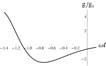
Figure 1: Time dependence of gravitational acceleration.

As one can see, the gravitational acceleration is weaker now than it used to be in the recent past. In the distant past, on the other hand, the gravitational force begins to oscillate. One should have in mind, however, that this picture drastically changes if the present time $t_{0}$ takes much larger values. Then, the period of oscillations grows beyond physical detection. In particular, the limit $t_{0}\to\infty$ turns the oscillatory behavior into a simple exponential law. Precisely, as one goes to the past, the attractive gravitational acceleration experiences exponentially fast growth.

V.2 Comparison with $\Lambda$CDM

The gravitational acceleration of a pointlike source in the $\Lambda$CDM background has the form

$$(g)_{\Lambda CDM}=-\frac{GM}{r^{2}_{\rm phys}}+\omega^{2}r_{\rm phys}\,.$$ (50)

Unfortunately, our expression Eq. (40) can never fully reduce to this form. What one can do is to make use of the fact that there is a range of distances for which the third term of Eq. (40), and the second term of Eq. (50) become dominant terms of their respective expressions. The integration constant $P_{0}$ is then determined from the requirement that these two dominant terms coincide at the present epoch. This leads to

$$P_{0}=\frac{2}{\omega\ell}\,.$$ (51)

The constant $P_{0}$, as defined by Eq. (51), ensures that the accelerated expansion predicted in this paper coincides with that of $\Lambda$CDM model.

Let me now calculate the turnaround radius of an arbitrarily chosen gravitational source, and compare it with the corresponding $\Lambda$CDM expression. The turnaround radius is defined as the distance from the pointlike source at which gravitational force drops to zero. In the type of theories we consider, the notion of turnaround radius is always well defined. Indeed, the gravitational force is attractive at small distances, whereas at large distances it becomes repulsive. Thus, there must exist the distance at which the gravitational acceleration takes zero value. It is calculated from the equation $g=0$, which reduces to

$$-\frac{1}{x^{2}}-\frac{Q}{x}+Px+J=0\,,$$

as seen from Eq. (40). I have already mentioned earlier that the last term in the above expression becomes important only at extremely large distances. Such large radii, however, are not met in the contemporary astronomical measurements. As a consequence, the term $J$ is shown to have a negligible influence on the value of $g$. The present epoch turnaround radius is then found by solving the equation

$$P_{0}\,x^{3}-Q_{0}\,x-1=0\,.$$ (52)

The general solution of cubic algebraic equations is well known, so that one straightforwardly obtains

$$x_{t}=\left(2P_{0}\right)^{-\frac{1}{3}}\left[\left(1+\sqrt{1-\sigma}\right)^{\frac{1}{3}}+\left(1-\sqrt{1-\sigma}\right)^{\frac{1}{3}}\right],$$ (53)

where $x_{t}$ denotes turnaround radius, and

$$\sigma\equiv\frac{4}{P_{0}}\!\left(\frac{Q_{0}}{3}\right)^{\!3}.$$ (54)

To estimate the range of values of $\sigma$, let me make use of the fact that no astronomical object in the observable Universe has mass larger than $\ell=10^{5}$ ly. This leads to $\sigma\gtrsim 5.25$, so that both square roots in Eq. (53) are imaginary. With this, the turnaround radius $x_{t}$ takes the form

$$x_{t}=\left(2P_{0}\right)^{-\frac{1}{3}}\left[\left(1+i\sqrt{\sigma-1}\right)^{\frac{1}{3}}+{\rm c.c.}\,\right].$$ (55)

The complicated expression Eq. (55) is simplified as follows. One starts with

$$1+i\sqrt{\sigma-1}\equiv\sqrt{\sigma}e^{i\varphi},$$

where $\varphi\equiv\arctan\sqrt{\sigma-1}$. Then, the turnaround radius $x_{t}$ is straightforwardly brought to the form

$$x_{t}\approx 0.62\cdot\cos\frac{\varphi}{3}\cdot\left(\omega\ell\right)^{\frac{1}{4}}.$$

This expression is further simplified by noticing that $\cos\frac{\varphi}{3}$ remains practically unchanged in the interval $\ell\in(0,10^{5})$ ly. Indeed, the constraint $\ell<10^{5}$ ly implies $\sigma\gtrsim 5.25$, which yields $1.12\lesssim\varphi<\pi/2$. As a consequence, $0.87\lesssim\cos\frac{\varphi}{3}\lesssim 0.93$, so that $\cos\frac{\varphi}{3}$ can approximately be considered a constant. Specifically, $\cos\frac{\varphi}{3}\approx 0.90\pm 0.03$ for all $\ell<10^{5}$ ly. The turnaround radius is then rewritten as

$$x_{t}\approx\left(0.56\pm 0.02\right)\cdot\left(\omega\ell\right)^{\frac{1}{4}}.$$ (56)

This formula holds true for all galaxy clusters and superclusters in the observable Universe. The corresponding $\Lambda$CDM expression is obtained by solving the equation $(g)_{\Lambda{\rm CDM}}=0$. It results in

$$(x_{t})_{\Lambda{\rm CDM}}\approx 0.79\cdot\left(\omega\ell\right)^{\frac{1}{3}}.$$ (57)

The comparison of Eq. (56) with Eq. (57) tells us that our turnaround radius does not agree with that of $\Lambda$CDM model. This is a consequence of the presence of MOND term in our expression for gravitational acceleration. One should have in mind though that there is still a possibility to change the form of the turnaround radius by making a different choice of the integration constant $P_{0}$. While this can ensure that the two turnaround radii become compatible, the accelerated expansion of the Universe will inevitably loose its $\Lambda$CDM form.

VI Concluding remarks

I have considered in this paper a class of cosmological models based on geometric sigma models with four scalar fields. These models have already been examined in Ref. 18 , where their regularity and stability have been proven. In this work, I search for spherically symmetric solutions, with the idea to check how additional four degrees of freedom modify Newtonian gravitational law.

The main result of my calculations is given by Eq. (40), which represents gravitational acceleration of a pointlike source in de Sitter background. In fact, the obtained result refers to the late time behavior of any cosmology with $\Lambda$CDM limit. There are four major terms in Eq. (40), which one by one, become dominant as the distance from the gravitational source grows. At short distances, the dominant contribution comes from the Newtonian term. As the distance grows, the dominant role is taken by the familiar MOND term. At even larger distances, the leading role is carried by the $\Lambda$CDM term which is responsible for the accelerated expansion of the Universe. Finally, the fourth term provides an extra repulsive acceleration that grows exponentially fast with distance. This term becomes significant only at extremely large distances that go beyond the observable Universe. As such, it is effectively neglected. The analysis has been done in a weak field approximation, with the help of an additional assumption that restrains the overall generality. Precisely, the field equations are solved with the help of the ansatz Eqs. (29) and (34) that basically truncated the infinite power series Eq. (17). Owing to this, the linearized field equations have been successfully solved. One should keep in mind, however, that the obtained solution is not as general as one would ideally like to have.

Another simplification used in this paper is the abandonment of the fourth term in Eq. (40). It has been explained that, in all observationally interesting situations, this term is too small. Let me clarify this statement. The term $J$ is positive, exponentially increasing function of $x$, which obviously becomes dominant for large enough $x$. In practice, however, the value of $x$ is bounded by the fact that the largest observed astronomical object has diameter of the order of $10^{8}$ ly. As a consequence, the distance $x$ is constrained by the inequality $x\lesssim 10^{-2}$. The cosmic time is also constrained. Indeed, the observable history of the Universe is defined by the finite interval $-1\lesssim\omega(t-t_{0})\leq 0$. With these restrictions, the argument of the function $J$ is found to satisfy $\sqrt{2}x/a\lesssim 0.04/a_{0}$, which straightforwardly leads to

$$J\lesssim 7$$

for all $t_{0}>0$. For higher values of the present time $t_{0}$, the term $J$ is constrained even more. Let me now compare $J$ with other terms in Eq. (40). The term $1/x^{2}$ is estimated with the help of the restriction $x\lesssim 10^{-2}$. It immediately gives

$$\frac{1}{x^{2}}\gtrsim 10^{4}\,,$$

which tells us that $J\ll 1/x^{2}$. The term $Q/x$ is estimated with the help of three observational restrictions. The first two are $x\lesssim 10^{-2}$ and $-1\lesssim\omega(t-t_{0})\leq 0$, while the third comes from the observation that no astronomical object in the observed Universe has mass larger than $\ell\sim 10^{5}$ ly. These three restrictions yield

$$\frac{Q}{x}\gtrsim 10^{5}\,,$$

and consequently, $J\ll Q/x$. Finally, let me estimate the term $Px$. It is immediately seen that $Px$ can be arbitrarily small if we restrict to small distances from the gravitational source. Notice, however, that the observed galaxies, galaxy clusters and superclusters are not pointlike objects. Instead, they have nonzero radii, which are related to their masses. The needed mass is the one which is distributed below the chosen distance $x$. A rough estimation of how $\ell$ is related to $x$ can be obtained in the spherically symmetric approximation in which matter density is considered constant. This assumption immediately leads to $\ell\propto x^{3}$, and consequently, $P_{0}\,x\propto 1/x^{2}$. Thus, the term $P_{0}\,x$ is bounded from below by the fact that $x\lesssim 10^{-2}$. The estimation of $Px$ is obtained when the restrictions $-1\lesssim\omega(t-t_{0})\leq 0$ and $\ell\lesssim 10^{5}$ ly are taken into account. One straightforwardly finds

$$Px\gtrsim 10^{3}\,,$$

so that $J\ll Px$. As we can see, $J$ is indeed negligible when compared to the other three terms in Eq. (40). The obtained estimation holds true when the present time $t_{0}$ obeys the inequality $t_{0}>0$. It applies to all the astronomical objects in the observable Universe.

To summarize, I have shown in this paper that observationally justified modifications of Newtonian gravity do not have to be imposed by hand. Instead, they can be found in already existing cosmological models. Specifically, I have examined a class of geometric sigma models whose late time behavior reduces to that of $\Lambda$CDM model. As it turns out, each of these models accommodates a spherically symmetric solution with the required MOND and $\Lambda$CDM modifications. Irrespective of this success, the present work is far from being complete. What remains to be done is to find the physical interpretation of the remaining physical degrees of freedom. This task, however, lies far beyond the scope of this paper.

- (1) J. C. Kapteyn, Astrophys. J. 55, 302 (1922).
- (2) J. H. Oort, Bulletin of the Astronomical Institutes of the Netherlands 6, 249 (1932).
- (3) F. Zwicky, Helvetica Physica Acta 6, 110 (1933).
- (4) F. Zwicky, Astrophys. J. 86, 217 (1937).
- (5) H.W. Babcock, Lick Observatory Bulletins 19, 41 (1939).
- (6) V. C. Rubin and W. K. Ford Jr., Astrophys. J. 159, 379 (1970).
- (7) V. C. Rubin, N. Thonnard and W. K. Ford Jr., Astrophys. J. 238, 471 (1980).
- (8) S. Capozziello and M. De Laurentis, Physics Reports 509, 167, (2011).
- (9) M. Vasilic, Class. Quant. Grav. 15, 29 (1998).
- (10) M. Vasilic, Phys. Rev. D 95, 123506 (2017).
- (11) V. Borka Jovanovic, S. Capozziello, P. Jovanovic and D. Borka, Phys. Dark Univ. 14, 73 (2016).
- (12) S. Capozziello, P. Jovanovic, V. Borka Jovanovic and D. Borka, JCAP 1706, 044 (2017).
- (13) M. Vasilic, Class. Quantum Grav. 35, 175015 (2018).
- (14) Xavier Calmet, Salvatore Capozziello and Daniel Pryer, Eur. Phys. J. C 77, 589 (2017).
- (15) M. Milgrom, Astrophys. J. 270, 365 (1983).
- (16) M. Milgrom, Astrophys. J. 270, 371 (1983).
- (17) B. Famaey and S. McGaugh, Living Rev. Relativity 15, 10 (2012).
- (18) R. H. Sanders and S. S. McGaugh, Ann. Rev. Astron. Astrophys. 40, 263 (2002).
- (19) J.D. Bekenstein, Contemp. Phys. 47, 387 (2006).
- (20) C. Skordis, Class. Quant. Grav. 26, 143001 (2009).
- (21) S. S. McGaugh and W. J. G. De Blok, Astrophys. J. 499, 66 (1998).
- (22) S. S. McGaugh, Phys. Rev. Lett. 106, 121303 (2011).
- (23) B. P. Abbott et al. [LIGO Scientific Collaboration, Virgo Collaboration], Phys. Rev. Lett. 116, 061102 (2016); 116, 221101 (2016); 116, 241103 (2016); Phys. Rev. X 6, 041015 (2016).
- (24) C. de Rham, J. T. Deskins, A. J. Tolley and S. Y. Zhou, Rev. Mod. Phys. 89, 025004 (2017).