Reconstruction of joint photon-number distributions of twin beams incorporating spatial noise reduction

Abstract

A method for reconstructing joint photon-number distributions of twin beams from the experimental photocount histograms is suggested and experimentally implemented. Contrary to the standard reconstruction methods, it incorporates spatial noise reduction based on spatial pairing of photons. Superior performance of the method above the usual one for the maximum-likelihood approach is demonstrated.

I Introduction

In classical optics, an optical field is characterized by its intensity and phase that is determined in an optical interferometer and is given with respect to certain reference phase Born and Wolf (1999). However, as the formulation of quantum theory of coherence Glauber (1963) revealed, the measurement of intensity represents only a certain limiting case appropriate for the characterization of intense optical fields. For weak optical fields composed of individual photons, the determination of a complete photocount (i.e. photo-electron) distribution is necessary Mandel and Wolf (1995). The Mandel detection formula Mandel and Wolf (1995) derived in the early days of quantum optics then provides the bridge between the measured photocount distribution and the distribution of (integrated) intensity that describes the analyzed field Peřina (1991).

Investigations of the detection of weak optical fields brought considerable attention to the role of noises present not only in the detection process but also in the observed optical fields Saleh (1978); Peřina (1991). The noise of a detector, that is composed of the intrinsic quantum shot-noise and an additional electronic noise, can be independently quantified and subsequently removed from the experimental data, at least in principle. Contrary to this, the optical noise superimposed to the observed optical field during its propagation to the detector cannot be usually eliminated and such noise is considered as a part of the optical field. However, this is not the case of twin beams that are composed of photon pairs Jedrkiewicz et al. (2004); Bondani et al. (2007); Blanchet et al. (2008); Brida et al. (2009a). The optical noise in a twin beam can be indirectly identified by exploiting spatial correlations of photons in a photon pair that naturally emerge during the generation of a twin beam Jost et al. (1998); Joobeur et al. (1994, 1996); Brambilla et al. (2004, 2010); Blanchet et al. (2008); Fedorov et al. (2008); Hamar et al. (2010); Tasca et al. (2013); Fickler et al. (2013, 2014); Jachura and Chrapkiewicz (2015). Such reduction of the noise may be useful whenever twin beams are applied, for instance in quantum metrology Lloyd (2008); Giovannetti et al. (2011), quantum imaging Pittman et al. (1995); Gatti et al. (2008); Brida et al. (2009b); Tasca et al. (2013) or quantum communications Saleh and Teich (1987).

Spatial correlations of photons in a twin beam are described by the intensity cross-correlation function that allows to define a correlated area Hamar et al. (2010). When an idler photon is detected inside the correlated area belonging to an already registered signal photon, both photons are considered as members of a single photon pair. This fact can be used to reduce the amount of noise present in the joint signal-idler photocount distribution obtained after the detection of a twin beam Peřina Jr. et al. (2017a). The strength of such noise reduction depends on the extension of a detection area in the idler beam, in which we expect the idler photon accompanying an already registered signal photon. The smaller the detection area is, the more efficient the noise reduction is. However, when the detection area is becoming smaller than the correlated area some idler photons do not fall into the detection area and so both photons from a photon pair cannot be simultaneously detected (’photon pairs are statistically partially broken’). Under these conditions, the noise reduction is becoming meaningless as it deforms the analyzed optical field. This process of noise reduction has been experimentally demonstrated in Peřina Jr. et al. (2017a) for a weak twin beam whose photocount distribution was monitored by an intensified CCD (iCCD) camera.

In this article we report on the development and experimental test of a reconstruction method for twin beams that takes advantage of the above discussed noise reduction. We show that the resulting photon-number distribution reached by the developed method is considerably less noisy compared to that obtained by the usual approach. For both reconstructions, we apply the method of maximum likelihood that has been considered as a workhorse for reconstructions of various types of quantum states. The idea of the discussed method is presented in Sec. II. Quantifiers monitoring the level of noise reduction due to spatial filtering are discussed in Sec. III. Sec. IV is devoted to practical implementation of the method. Conclusions are drawn in Sec. V.

II Reconstruction of twin-beam photon-number distributions incorporating spatial noise reduction

We present the developed method by its comparison with the usual reconstruction method. In the usual approach, a measured joint signal-idler photocount histogram $f(c_{\rm s},c_{\rm i})$ that gives the probability of detecting together $c_{\rm s}$ signal and $c_{\rm i}$ idler photocounts from one realization of a twin beam is directly used in the reconstruction formula. In the maximum-likelihood approach, the joint signal-idler photon-number distribution $p^{\rm std}(n_{\rm s},n_{\rm i})$ of the reconstructed twin beam is reached as a steady state of the following iteration procedure ($l=0,1,\ldots$) Dempster et al. (1977); Řeháček et al. (2003); Peřina Jr. et al. (2012a); Harder et al. (2014):

$$p^{(l+1)}(n_{\rm s},n_{\rm i}) = p^{(l)}(n_{\rm s},n_{\rm i})$$ (1)

$$\mbox{}\times\sum_{c_{\rm s},c_{\rm i}}\frac{f(c_{\rm s},c_{\rm i})T_{\rm s}(c_{\rm s},n_{\rm s})T_{\rm i}(c_{\rm i},n_{\rm i})}{\sum_{n^{\prime}_{s},n^{\prime}_{i}}T_{\rm s}(c_{\rm s},n^{\prime}_{\rm s})T_{\rm i}(c_{\rm i},n^{\prime}_{\rm i})p^{(l)}(n^{\prime}_{\rm s},n^{\prime}_{\rm i})}.$$

In Eq. (1), the positive-operator-valued measures (POVMs) $T_{a}(c_{a},n_{a})$ give the probabilities for detecting $c_{a}$ photocounts out of $n_{a}$ photons in beam $a$, $a={\rm s,i}$. As such they characterize a linear relation between the (reconstructed) joint signal-idler photon-number distribution $p$ and the corresponding experimental photocount histogram $f$. This relation is ’inverted’ with the help of the formula written in Eq. (1). The form of POVMs depends on the properties of a detector. For the used iCCD camera, detection efficiency, mean dark count number per pixel and number of pixels inside an active detection area are the parameters entering the formulas for POVMs $T_{a}(c_{a},n_{a})$ occurring in Eq. (1) [see below in Eq. (14)]. We note that the iteration procedure corrects for the detrimental effects in detection described explicitly in the POVMs including the detector noise.

Contrary to this, the suggested method exploits filtering based on spatial correlations Peřina Jr. et al. (2017a) to arrive at a histogram $f_{\rm p}(c_{\rm p};m_{\rm d})$ of paired signal and idler photocounts and a joint histogram $f_{\rm si}^{\rm unp}(c_{\rm s},c_{\rm i};m_{\rm d})$ of unpaired photocounts that occur in the neighborhood (inside the detection area) of the identified photocount pairs. Details of identification of individual photocounts and different types of photocount configurations in both signal and idler detection strips are found in the caption to Fig. 1.

Figure 1: Typical detection configuration in the signal and idler detection strips on a photocathode of the iCCD camera showing one photocount in the signal strip and 3 photocounts in the idler strip. The photocount in the middle of the idler strip is positioned within the correlated area (that covers $m_{\rm c}$ pixels) drawn around the point corresponding to the detection position of the photocount in the signal strip and so both photocounts form a photocount pair. For given number $m_{\rm d}$ of pixels in the detection area, the photocount in the upper part of the idler strip lies inside the detection area and so it is considered as an unpaired photocount in the reconstruction procedure. Contrary to this, the photocount in the lower part of the idler strip lies outside the detection area and so it is identified as a noise unpaired photocount and as such it is excluded from the consideration in the reconstruction procedure. The extension of the detection area characterized by $m_{\rm d}$ pixels gradually changes and optimal performance of the reconstruction procedure is expected for $m_{\rm d}^{0}\approx m_{\rm c}$. The signal (idler) strip is composed of $N_{\rm s}$ ($N_{\rm i}$) pixels.

Both histograms $f_{\rm p}(c_{\rm p};m_{\rm d})$ and $f_{\rm si}^{\rm unp}(c_{\rm s},c_{\rm i};m_{\rm d})$ depend on the extension of the detection area that, in case of CCD detection elements, is conveniently parameterized by the number $m_{\rm d}$ of pixels inside this area. Reconstruction of both fields described by the histograms $f_{\rm p}(c_{\rm p};m_{\rm d})$ and $f_{\rm si}^{\rm unp}(c_{\rm s},c_{\rm i};m_{\rm d})$ is based upon the iteration procedure of Eq. (1) (and its one-dimensional variant) in which the noiseless POVMs $T_{a}^{\rm nl}(c_{a},n_{a})$ are used [see Eq. (14) below, $D=0$]. We note that the noiseless POVMs are applied as the noise is assumed to be (partially) removed by filtering via spatial correlations. The usual detection efficiencies $\eta_{\rm s}$ and $\eta_{\rm i}$ appropriate for the signal and idler beam (detection strip), respectively, are used in reconstructing the joint signal-idler photon-number distribution $p_{\rm si}^{\rm unp}(n_{\rm s},n_{\rm i};m_{\rm d})$ from the histogram $f_{\rm si}^{\rm unp}(c_{\rm s},c_{\rm i};m_{\rm d})$ of unpaired photocounts. Contrary to this, an effective detection efficiency $\eta_{\rm p}(m_{\rm d})$ has to be applied when reconstructing the distribution $p_{\rm p}$ of photon pairs from the histogram $f_{\rm p}(c_{\rm p};m_{\rm d})$. Provided that the positions of signal photocounts in the signal detections strip are used to define the overall detection area in the idler detection strip that is taken into account for the spatial filtering, the effective detection efficiency $\eta_{\rm i,p}^{\rm eff}$ is given as (for more details, see Peřina Jr. et al. (2017a))

$$\eta_{\rm i,p}^{\rm eff}(m_{\rm d})=\frac{\langle c_{\rm i}\rangle^{\rm red}(m_{\rm d})}{\langle c_{\rm i}\rangle}\eta_{\rm s},$$ (2)

where $\langle c_{\rm i}\rangle^{\rm red}(m_{\rm d})$ [$\langle c_{\rm i}\rangle$] gives the mean number of idler photocounts considered with [without] spatial filtering. For the detection area with $m_{\rm d}$ pixels, an overall joint signal-idler photon-number distribution $p(n_{\rm s},n_{\rm i};m_{\rm d})$ is obtained by the following convolution:

$$p(n_{\rm s},n_{\rm i};m_{\rm d}) = \sum_{n_{\rm p}=0}^{\min(n_{\rm s},n_{\rm i})}p_{\rm p}(n_{\rm p};m_{\rm d})$$ (3)

$$\mbox{}\times p_{\rm si}^{\rm unp}(n_{\rm s}-n_{\rm p},n_{\rm i}-n_{\rm p};m_{\rm d})$$

and the distribution $p_{\rm p}$ is derived from the histogram $f_{\rm p}$. Proper choice of the number $m_{\rm d}^{0}$ of pixels in the detection area then identifies the joint photo-number distribution $p(n_{\rm s},n_{\rm i};m_{\rm d}^{0})$ of the reconstructed twin beam.

III Quantifiers useful for monitoring the level of noise reduction

To monitor the performance of the noise reduction in the suggested reconstruction method, we need to quantify (quantum) correlations between the signal and idler fields both for the experimental photocounts and reconstructed photon numbers. Here, we show that the non-classicality depths $\tau$ Lee (1991) determined for the non-classicality identifiers $E_{k}$, $k=2,3,4$, defined in terms of intensity moments $\langle W^{l}\rangle$ as Peřina Jr. et al. (2017b)

$$E_{2} = \langle W_{\rm s}^{2}\rangle+\langle W_{\rm i}^{2}\rangle-2\langle W_{\rm s}W_{\rm i}\rangle,$$ (4)

$$E_{3} = \langle W_{\rm s}^{3}\rangle+\langle W_{\rm i}^{3}\rangle-\langle W_{\rm s}^{2}W_{\rm i}\rangle-\langle W_{\rm s}W_{\rm i}^{2}\rangle,$$ (5)

$$E_{4} = \langle W_{\rm s}^{4}\rangle+\langle W_{\rm i}^{4}\rangle-2\langle W_{\rm s}^{2}W_{\rm i}^{2}\rangle$$ (6)

allow for relatively precise determination of the number $m_{\rm d}^{0}$ of detection pixels in the detection area that leads to the best result of the reconstruction procedure. We note that an $l$-th intensity moment $\langle W^{l}\rangle$ is related to the moments $\langle c^{k}\rangle$ of photocounts by the formula $\langle W^{l}\rangle=\sum_{k=1}^{l}S_{lk}^{-1}\langle c^{k}\rangle$ that uses the Stirling numbers $S_{lk}$ of the second kind. We remind that a non-classicality depth $\tau$ is given by the number of thermal photons needed to conceal nonclassical properties of an optical field visible in a given non-classicality identifier Peřina Jr. et al. (2017b). For comparison, we also determine the traditional covariance $C_{\Delta c}$ of fluctuations of the numbers $c_{\rm s}$ and $c_{\rm i}$ of the signal and idler photocounts and sub-shot-noise parameter $R_{c}$,

$$C_{\Delta c} = \frac{\langle\Delta c_{\rm s}\Delta c_{\rm i}\rangle}{\sqrt{\langle(\Delta c_{\rm s})^{2}\rangle\langle(\Delta c_{\rm i})^{2}\rangle}},$$ (7)

$$R_{c} = \frac{\langle[\Delta(c_{\rm s}-c_{\rm i})]^{2}\rangle}{\langle c_{\rm s}\rangle+\langle c_{\rm i}\rangle}.$$ (8)

IV Experimental implementation of the developed reconstruction method

To compare the performance of the suggested reconstruction method with the standard one, we measured a joint signal-idler photocount histogram $f$ of a twin beam centered at the wavelength 560 nm and originating in a non-collinear type-I interaction in a 5-mm long BaB₂O₄ crystal pumped by the third harmonics of a femtosecond cavity dumped Ti:sapphire laser (pulse duration 150 fs, central wavelength 840 nm) Hamar et al. (2010). The signal and idler photocounts were captured in different detection strips on a photocathode of an iCCD camera Andor DH334-18U-63 (for the geometry of experimental setup, see Fig. 2); $1.2\times 10^{6}$ experimental repetitions were performed.

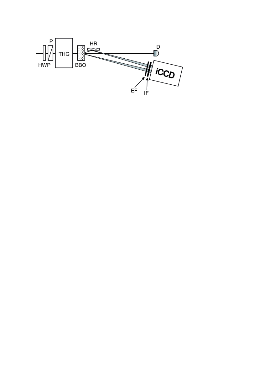
Figure 2: Scheme of the experiment. The third harmonics (THG, 280 nm) of a Ti:sapphire laser beam pumps a BaB₂O₄ (BBO) nonlinear crystal. Nearly degenerate signal and idler (steered by high-reflectivity mirror HR) beams are filtered by a 14-nm-wide bandpass frequency filter IF and then detected in two detection strips on a photocathode of iCCD camera. Long-pass (above 490 nm) filter EF diminishes the noise. Intensity of the pump beam monitored by detector D is actively stabilized (rms below 0.3%) using motorized half-wave plate HWP followed by polarizer P. According to the calibration procedure Peřina Jr. et al. (2012b) applied to the experimental data, the signal (idler) detection strip was composed of $N_{\rm s}=N_{\rm i}=6500$ pixels, exhibited detection efficiency $\eta_{\rm s}=0.228\pm 0.005$ ($\eta_{\rm i}=0.223\pm 0.005$) and suffered by $D_{\rm s}=0.2/N_{\rm s}$ ($D_{\rm i}=0.2/N_{\rm i}$) mean dark count number per pixel.

Provided that a detection strip is composed of $N$ pixels, has detection efficiency $\eta$ and its mean dark count number per pixel is $D$, its POVM $T$ needed in Eq. (1) for the reconstruction procedure is written as Peřina Jr. et al. (2012a):

$$T(c,n) = \left(\begin{array}[]{c}N\\ c\end{array}\right)(1-D)^{N}(1-\eta)^{n}(-1)^{c}$$ (14)

$$\mbox{}\times\sum_{l=0}^{c}\left(\begin{array}[]{c}c\\ l\end{array}\right)\frac{(-1)^{l}}{(1-D)^{l}}\left(1+\frac{l}{N}\frac{\eta}{1-\eta}\right)^{n}.$$

In the suggested method, reduction of the noise in the experimental data is achieved by spatial filtering of the photocounts whose strength gradually increases with the decreasing number $m_{\rm d}$ of pixels in the considered detection areas drawn around the identified photocount pairs. This leads both to the decrease of the number $\langle c_{p}\rangle$ of identified photocount pairs as well as the decrease of the numbers $\langle c_{\rm s}\rangle$ and $\langle c_{\rm i}\rangle$ of the signal and idler photocounts found inside these detection areas. The essence of the suggested method is based on the fact that the numbers $\langle c_{\rm s}\rangle$ and $\langle c_{\rm i}\rangle$ decrease relatively faster than the number $\langle c_{p}\rangle$ with decreasing number $m_{\rm d}$ of detection pixels. So, the signal-to-noise ratios $S_{a}\equiv\langle c_{p}\rangle/\langle c_{a}\rangle$, $a={\rm s,i}$, increase with decreasing $m_{\rm d}$. For the analyzed experimental data and following the curves in Fig. 3(a), we have $S_{a}\approx 10$, $a={\rm s,i}$, for $m_{\rm d}^{0}=290$ compared to $S_{a}\approx 4$ determined without spatial filtering. We note that, for our experimental data, the detection area with $m_{\rm d}^{0}=290$ pixels just covers the correlated area whose profile can also be deduced from the obtained data (for details, see Peřina Jr. et al. (2017a)). Thus, the signal-to-noise ratios are improved more than two times by the filtering.

(a)   

(b)   

(c)   

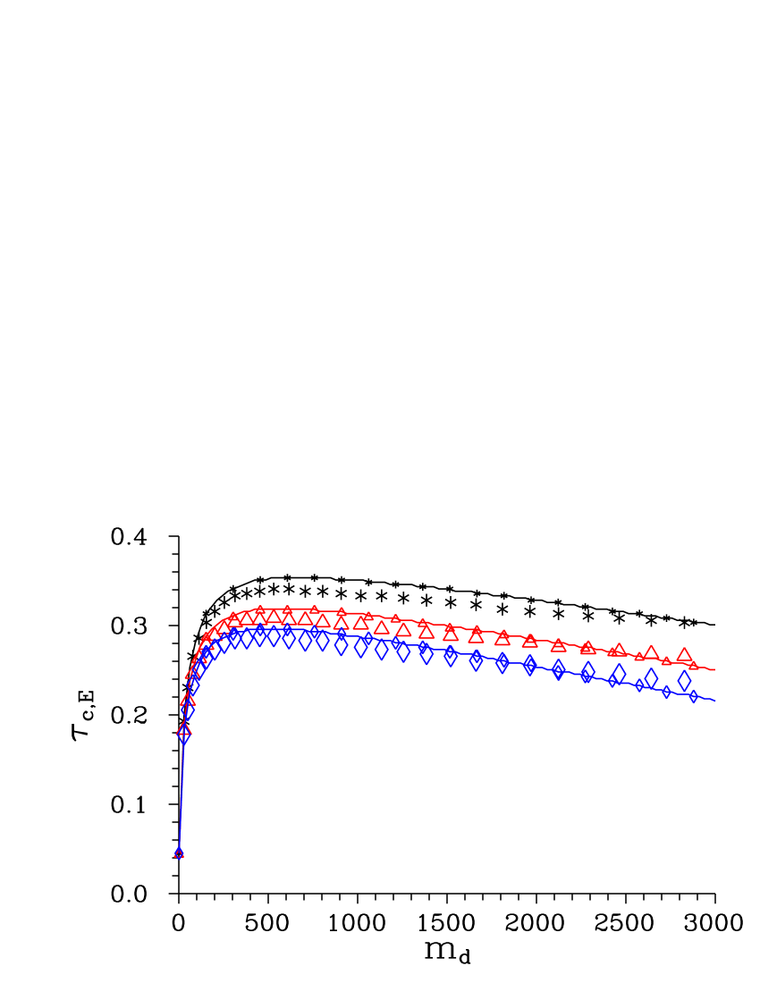
Figure 3: (a) Signal-to-noise ratios $S_{a}\equiv\langle c_{p}\rangle/\langle c_{a}\rangle$ for $a={\rm s}$ ($\ast$) and $a={\rm i}$ ($\triangle$), (b) covariance $C_{\Delta c}$ ($\ast$) and sub-shot-noise parameter $R_{c}$ ($\triangle$) and (c) non-classicality depths $\tau_{c,E_{k}}$ for $k=2$ ($\ast$), 3 (red $\triangle$) and 4 (blue $\diamond$) determined from the photocount measurement as they depend on the number $m_{\rm d}$ of pixels in the detection area. Experimental values are plotted as isolated symbols, the corresponding solid curves were drawn following the standard model of Ref. Peřina Jr. et al. (2017a). Relative experimental errors for $S_{\rm s}$, $S_{\rm i}$, $C_{\Delta c}$, $R_{c}$, $\tau_{c,E_{2}}$, $\tau_{c,E_{3}}$, and $\tau_{c,E_{4}}$ are lower than in turn 1%, 1%, 3%, 3%, 2%, 3% and 4%.

Spatial filtering improves correlations between the signal and idler photocount numbers. In case of the covariance $C_{\Delta c}$ of the fluctuations of the signal and idler photocount numbers and the corresponding sub-shot-noise parameter $R_{c}$ defined in Eqs. (7) and (8), respectively, these quantities tend to reach their optimal values for the negligibly small detection area ($C_{\Delta c}\rightarrow 1$, $R_{c}\rightarrow 0$ for $m_{\rm d}\rightarrow 0$), as documented in Fig. 3(b). In contrast to this and according to the curves of Fig. 3(c), the non-classicality depths $\tau_{c,E_{k}}$ belonging to the non-classicality identifiers $E_{k}$, $k=2,3,4$, from Eqs. (4—6) reach their maximal values in the range of $m_{\rm d}$ where the detection area approximately coincides with the correlated area. The values of $\tau_{c,E_{k}}$ rapidly drop down to zero when the detection area becomes smaller than the correlated area. For this reason, the non-classicality depths $\tau_{c,E_{k}}$ are qualitatively better for monitoring the process of spatial filtering. Also, the non-classicality identifiers $E_{2}$, $E_{3}$ and $E_{4}$ that are in turn based on the second-, third- and fourth-order intensity moments behave similarly in the process of spatial filtering. This indicates that the spatial filtering systematically modifies correlations of different orders.

Now let us have a look how these modifications in the experimental photocount histograms affect the behavior of correlations in the reconstructed photon-number distributions. The determination of the effective detection efficiency $\eta_{\rm i,p}^{\rm eff}$ (or $\eta_{\rm s,p}^{\rm eff}$) that is used for reconstructing the paired part of the photocount field represents the most important (though technical) step in the whole reconstruction. These effective efficiencies naturally decrease with the decreasing number $m_{\rm d}$ of detection pixels and they attain values around $\eta_{\rm s}\eta_{\rm i}$ when the detection area is close to the correlated area (see Fig. 4). These values are then used to arrive at the proper photon-number distribution of the analyzed twin beam.

Figure 4: Effective efficiencies $\eta_{\rm s,p}^{\rm eff}$ ($\ast$) and $\eta_{\rm i,p}^{\rm eff}$ ($\triangle$) defined in Eq. (2) as they depend on the number $m_{\rm d}$ of pixels in the detection area. Experimental values are plotted as isolated symbols, the corresponding solid curves were drawn following the standard model of Ref. Peřina Jr. et al. (2017a). Relative experimental errors are better than 2%.

Properties of a joint signal-idler photon-number distribution $p$ reached by the reconstruction method depend on the strength of the spatial filtering, as documented in Fig. 5 where the most important quantities of the reconstructed twin beam are plotted as functions of the number $m_{\rm d}$ of pixels in the detection areas.

(a)   

(b)   

(c)   

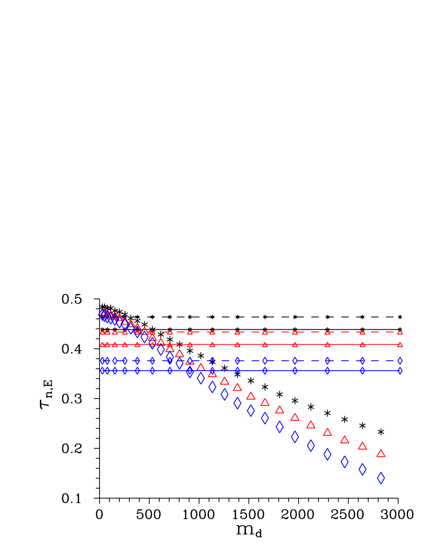
Figure 5: (a) Mean photon number $\langle n\rangle\equiv(\langle n_{\rm s}\rangle+\langle n_{\rm i}\rangle)/2$ ($\ast$), (b) covariance $C_{\Delta n}$ ($\ast$) and sub-shot-noise parameter $R_{n}$ ($\triangle$) and (c) non-classicality depths $\tau_{n,E_{k}}$ for k=2 ($\ast$), 3 (red $\triangle$) and 4 (blue $\diamond$) determined for the reconstructed twin beam are plotted as isolated symbols for different numbers $m_{\rm d}$ of pixels in the detection area. Horizontal lines give the values reached by the standard reconstruction method with POVMs including the intrinsic detector mean dark count numbers ($D_{a}N_{a}=0.2$, $a={\rm s,i}$; solid lines) and suitably increased mean dark count numbers ($D_{a}N_{a}=0.45$, $a={\rm s,i}$; dashed lines). Relative experimental errors for $\langle n\rangle$, $C_{\Delta n}$, $R_{n}$, $\tau_{n,E_{2}}$, $\tau_{n,E_{3}}$, and $\tau_{n,E_{4}}$ are lower than in turn 1%, 3%, 3%, 2%, 3% and 4%.

According to the curves of Fig. 5(a), the mean photon-number $\langle n\rangle$ [$\langle n\rangle=(\langle n_{\rm s}\rangle+\langle n_{\rm i}\rangle)/2$] of the reconstructed twin beam slightly decreases with the increasing spatial filtering. However, it starts to increase when the detection area is comparable to the correlated area. The initial decrease of the mean photon-number $\langle n\rangle$ with decreasing number $m_{\rm d}$ observed for greater numbers $m_{\rm d}$ has two reasons. First, the unwanted noise present in the experimental data is gradually removed. Second, the number $\langle c_{\rm p}\rangle(m_{\rm d})$ of identified photocount pairs is greater than the actual one due to the existence of accidental photocount pairs (for details, see Peřina Jr. et al. (2017a)) on the one hand, on the other hand the corresponding effective detection efficiency $\eta_{\rm s,p}^{\rm eff}$ that is constructed to compensate for the effect of accidental pairing is slightly overestimated. In our experiment, both contributions are comparably strong. Whereas the first effect just demonstrates the essence of the spatial noise reduction, the second effect distorts the experimental data and as such it is unwanted. However, this effect is minimal (and ideally disappears) when the detection area just covers the correlated area. In this case, the number of accidental photocount pairs is already very low and, according to the theory of absolute detector calibration Klyshko (1980), the definition (2) of the effective detection efficiency $\eta_{\rm i,p}^{\rm eff}$ gives us $\eta_{\rm i,p}^{\rm eff}\approx\eta_{\rm s}^{2}$. The appropriate number $m_{\rm d}^{0}$ of pixels in the detection area is ideally revealed by determining the correlated area (or even more precisely by determining the profile of the correlated area Peřina Jr. et al. (2017a)).

The reconstructed fields are naturally endowed with better covariances $C_{\Delta n}$ of the fluctuations of photon numbers compared to the original covariances $C_{\Delta c}$ of the fluctuations of photocount numbers, as evidenced by comparing the graphs in Figs. 3(b) and 5(b). On the other hand, direct comparison of sub-shot-noise parameters $R_{n}$ and $R_{c}$ as well as non-classicality depths $\tau_{n,E_{k}}$ and $\tau_{c,E_{k}}$ for $k=2,3,4$ belonging both to photocount and photon-number fields is not possible as the reconstructed fields are roughly four times more intense. On the other hand, mutual comparison of the curves for non-classicality depths $\tau_{c,E_{k}}$ and $\tau_{n,E_{k}}$ drawn in Figs. 3(c) and 5(c) reveals qualitatively different behavior of these depths in the area of $m_{\rm d}$ where the detection area is comparable or smaller than the correlated area. This difference comes from the fact that the reconstruction method treats differently photocount pairs and individual noisy (unpaired) photocounts. Roughly speaking the photocount pairs are amplified stronger (as $1/\eta_{\rm s,p}^{\rm eff}$) than the individual noisy photocounts (as $1/\eta_{\rm s}$) in the reconstruction method. We note that, in our experiment, we have $\eta_{\rm s,p}^{\rm eff}(m_{\rm d}^{0}=290)\approx 0.04$ compared to $\eta_{\rm s}\approx 0.2$.

The analysis of the experimental data revealed the correlated area with 290 pixels (for details, see Peřina Jr. et al. (2017a)). The reconstructed joint signal-idler photon-number distribution $p$ obtained for $m_{\rm d}^{0}=290$ pixels in the detection area, that we consider as the best from the point of view of the developed method, is shown in Fig. 6(a). For comparison, we draw in Fig. 6(b) a photon-number distribution $p^{\rm std}$ reached by the standard reconstruction method that includes the intrinsic detector mean dark count numbers $D_{\rm s}$ and $D_{\rm i}$ as specified in the caption to Fig. 2.

(a)   

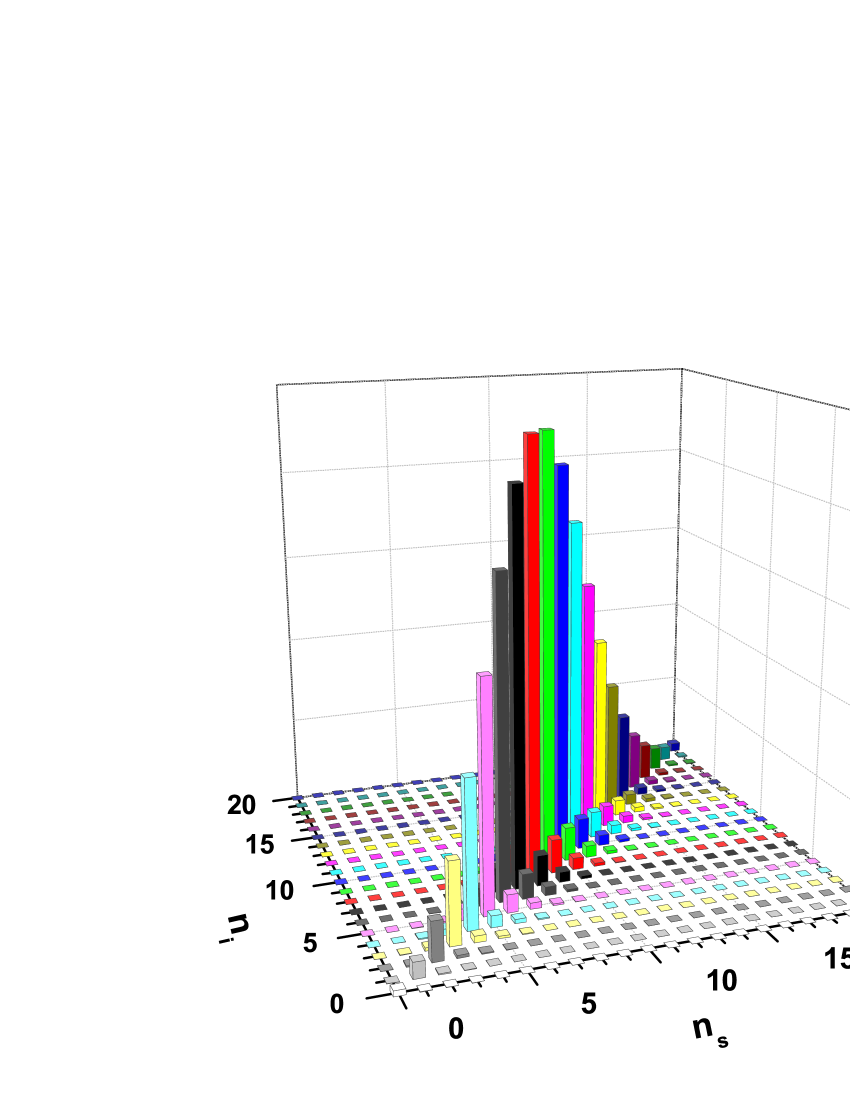
(b)   

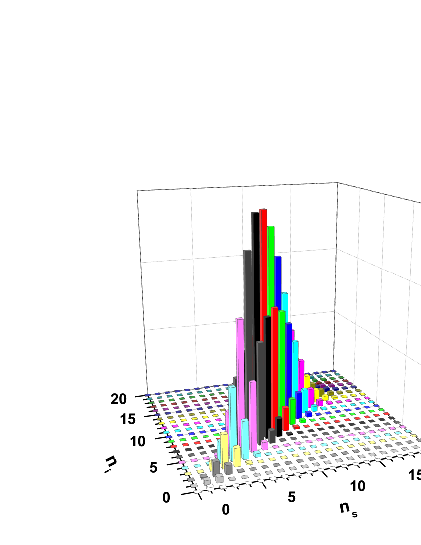
Figure 6: Joint signal-idler photon-number distribution $p$ of the reconstructed twin beam reached (a) with the help of filtering by spatial correlations and (b) by the standard reconstruction procedure.

Values of the parameters $\langle n\rangle$, $C_{\Delta n}$, $R_{n}$ and $\tau_{n,E_{k}}$, $k=2,3,4$, of this standardly reconstructed twin beam, that are plotted in Figs. 5(a)—(c) by solid horizontal lines, show that the mean photon-number $\langle n\rangle$ is about 15% larger and the noise in this twin beam is also larger compared to the twin beam revealed by the developed reconstruction method. The greater mean photon-number $\langle n\rangle$ indicates that considerable amount of the optical noise is present in the original (i.e. not spatially filtered) experimental photocount histogram. This amount of optical noise can phenomenologically be removed in the standard reconstruction procedure by considering greater (effective) values of the mean dark count numbers $D_{\rm s}$ and $D_{\rm i}$. To demonstrate the performance of this approach, we have plotted by dashed horizontal lines in the graphs of Figs. 5(a)—(c) the values of parameters appropriate for $D_{\rm s}N_{\rm s}=D_{\rm i}N_{\rm i}=0.45$. The chosen amount of the optical noise approximately leads to the correct mean photon-number $\langle n\rangle$, but the values of non-classicality depths $\tau_{n,E_{k}}$, $k=2,3,4$, remain worse in comparison with those characterizing the reconstructed twin beam in Fig. 6(a). Detailed analysis of the curves plotted in Fig. 5(c) reveals that the greater the power of intensity moments involved in the determination of the non-classicality depth $\tau_{n,E_{k}}$, the worse the noise reduction by the standard reconstruction procedure compared to the developed method. These results clearly show that the suggested reconstruction method exploiting filtering by spatial correlations is superior above the standard one.

V Conclusions

We have suggested and elaborated a method for reconstructing joint photon-number distributions of twin beams from the measured photocount histograms that uses spatial filtering of the experimental photocounts to reduce the experimental noise. The applied filtering exploits spatial correlations of photons in a twin beam. In the experimental implementation, we demonstrated superior performance of the developed reconstruction method above the standard one. Though the processing of experimental data in the developed method is considerably more involved in comparison with the standard approach, the developed method brings considerable advantages and we suggest its application wherever the spatially resolved photocount histograms of twin beams are at disposal.

VI Acknowledgments

The authors thank M. Hamar for his help with the experiment. O.H. and V.M. were supported by the GA ČR project 18-08874S. J.P. was supported by the GA ČR project 18-22102S.

References

- Born and Wolf (1999) M. Born and E. Wolf, Principles of Optics (Cambridge Univ. Press., Cambridge, 7th Ed.-, 1999).
- Glauber (1963) R. J. Glauber, “Coherent and incoherent states of the radiation field,” Phys. Rev. 131, 2766—2788 (1963).
- Mandel and Wolf (1995) L. Mandel and E. Wolf, Optical Coherence and Quantum Optics (Cambridge Univ. Press, Cambridge, 1995).
- Peřina (1991) J. Peřina, Quantum Statistics of Linear and Nonlinear Optical Phenomena (Kluwer, Dordrecht, 1991).
- Saleh (1978) B. E. A. Saleh, Photoelectron Statistics (Springer-Verlag, New York, 1978).
- Jedrkiewicz et al. (2004) O. Jedrkiewicz, Y. K. Jiang, E. Brambilla, A. Gatti, M. Bache, L. A. Lugiato, and P. Di Trapani, “Detection of sub-shot-noise spatial correlation in high-gain parametric down-conversion,” Phys. Rev. Lett. 93, 243601 (2004).
- Bondani et al. (2007) M. Bondani, A. Allevi, G. Zambra, M. G. A. Paris, and A. Andreoni, “Sub-shot-noise photon-number correlation in a mesoscopic twin beam of light,” Phys. Rev. A 76, 013833 (2007).
- Blanchet et al. (2008) J.-L. Blanchet, F. Devaux, L. Furfaro, and E. Lantz, “Measurement of sub-shot-noise correlations of spatial fluctuations in the photon-counting regime,” Phys. Rev. Lett. 101, 233604 (2008).
- Brida et al. (2009a) G. Brida, L. Caspani, A. Gatti, M. Genovese, A. Meda, and I. R. Berchera, “Measurement of sub-shot-noise spatial correlations without backround subtraction,” Phys. Rev. Lett. 102, 213602 (2009a).
- Jost et al. (1998) B. M. Jost, A. V. Sergienko, A. F. Abouraddy, B. E. A. Saleh, and M. C. Teich, “Spatial correlations of spontaneously down-converted photon pairs detected with a single-photon-sensitive CCD camera,” Opt. Express 3, 81—88 (1998).
- Joobeur et al. (1994) A. Joobeur, B. E. A. Saleh, and M. C. Teich, “Spatiotemporal coherence properties of entangled light beams generated by parametric down-conversion,” Phys. Rev. A 50, 3349—3361 (1994).
- Joobeur et al. (1996) A. Joobeur, B. E. A. Saleh, T. S. Larchuk, and M. C. Teich, “Coherence properties of entangled light beams generated by parametric down-conversion: Theory and experiment,” Phys. Rev. A 53, 4360—4371 (1996).
- Brambilla et al. (2004) E. Brambilla, A. Gatti, M. Bache, and L. A. Lugiato, “Simultaneous near-field and far-field spatial quantum correlations in the high-gain regime of parametric down-conversion,” Phys. Rev. A 69, 023802 (2004).
- Brambilla et al. (2010) E. Brambilla, L. Caspani, L. A. Lugiato, and A. Gatti, “Spatiotemporal structure of biphoton entanglement in type-II parametric down-conversion,” Phys. Rev. A 82, 013835 (2010).
- Fedorov et al. (2008) M. V. Fedorov, M. A. Efremov, P. A. Volkov, E. V. Moreva, S. S. Straupe, and S. P. Kulik, “Spontaneous parametric down-conversion: Anisotropical and anomalously strong narrowing of biphoton momentum correlation distributions,” Phys. Rev. A 77, 032336 (2008).
- Hamar et al. (2010) M. Hamar, J. Peřina Jr., O. Haderka, and V. Michálek, “Transverse coherence of photon pairs generated in spontaneous parametric down-conversion,” Phys. Rev. A 81, 043827 (2010).
- Tasca et al. (2013) D. S. Tasca, R. S. Aspden, P. A. Morris, G. Anderson, R. W. Boyd, and M. J. Padgett, “The influence of non-imaging detector design on heralded ghost-imaging and ghost-diffraction examined using a triggered iCCD camera,” Opt. Express 21, 30460 (2013).
- Fickler et al. (2013) R. Fickler, M. Krenn, R. Lapkiewicz, S. Ramelow, and A. Zeilinger, “Real-time imaging of quantum entanglement,” Sci. Rep. 3, 1914 (2013).
- Fickler et al. (2014) R. Fickler, R. Lapkiewicz, S. Ramelow, and A. Zeilinger, “Quantum entanglement of complex photon polarization patterns in vector beams,” Phys. Rev. A 89, 060301(R) (2014).
- Jachura and Chrapkiewicz (2015) M. Jachura and R. Chrapkiewicz, “Shot-by-shot imaging of Hong -Ou- Mandel interference with an intensified sCMOS camera,” Opt. Lett 40, 1540—1543 (2015).
- Lloyd (2008) S. Lloyd, “Enhanced sensitivity of photodetection via quantum illumination,” Science 321, 1463—1465 (2008).
- Giovannetti et al. (2011) V. Giovannetti, S. Lloyd, and L. Maccone, “Advances in quantum metrology,” Nature Phot. 5, 222—229 (2011).
- Pittman et al. (1995) T. B. Pittman, Y. H. Shih, D. V. Strekalov, and A. V. Sergienko, “Optical imaging by means of two-photon quantum entanglement,” Phys. Rev. A 52, R3429—R3432 (1995).
- Gatti et al. (2008) A. Gatti, E. Brambilla, and L. Lugiato, “Quantum imaging,” in Progress in Optics, Vol. 51, edited by E. Wolf (Elsevier, Amsterdam, 2008) pp. 251—348.
- Brida et al. (2009b) G. Brida, A. Meda, M. Genovese, E. Predazzi, and I. Ruo-Berchera, “Systematic study of the PDC speckle structure for quantum imaging applications,” J. Mod. Opt. 56, 201—208 (2009b).
- Saleh and Teich (1987) B. E. A. Saleh and M. C. Teich, “Can the channel capacity of a light-wave communication system be increased by the use of photon-number-squeezed light?” Phys. Rev. Lett. 58, 2656–2659 (1987).
- Peřina Jr. et al. (2017a) J. Peřina Jr., V. Michálek, and O. Haderka, “Noise reduction in photon counting by exploiting spatial correlations,” Phys. Rev. Appl. 8, 044018 (2017a).
- Dempster et al. (1977) A. P. Dempster, N. M. Laird, and D. B. Rubin, “Maximum likelihood from incomplete data via the EM algorithm,” J. R. Statist. Soc. Ser. B 39, 1—38 (1977).
- Řeháček et al. (2003) J. Řeháček, Z. Hradil, O. Haderka, J. Peřina Jr., and M. Hamar, “Multiple-photon resolving fiber-loop detector,” Phys. Rev. A 67, 061801(R) (2003).
- Peřina Jr. et al. (2012a) J. Peřina Jr., M. Hamar, V. Michálek, and O. Haderka, “Photon-number distributions of twin beams generated in spontaneous parametric down-conversion and measured by an intensified CCD camera,” Phys. Rev. A 85, 023816 (2012a).
- Harder et al. (2014) G. Harder, C. Silberhorn, J. Řehácek, Z. Hradil, L. Mot́ka, B. Stoklasa, and L. L. Sanchez-Soto, “Time-multiplexed measurements of nonclassical light at telecom wavelengths,” Phys. Rev. A 90, 042105 (2014).
- Lee (1991) C. T. Lee, “Measure of the nonclassicality of nonclassical states,” Phys. Rev. A 44, R2775—R2778 (1991).
- Peřina Jr. et al. (2017b) J. Peřina Jr., I. I. Arkhipov, V. Michálek, and O. Haderka, “Non-classicality and entanglement criteria for bipartite optical fields characterized by quadratic detectors,” Phys. Rev. A 96, 043845 (2017b).
- Peřina Jr. et al. (2012b) J. Peřina Jr., O. Haderka, M. Hamar, and V. Michálek, “Absolute detector calibration using twin beams,” Opt. Lett. 37, 2475—2477 (2012b).
- Klyshko (1980) D. N. Klyshko, “Use of two-photon light for absolute calibration of photoelectric detectors,” Sov. J. Quantum Electron. 10, 1112 –1117 (1980).