A note on solving nonlinear optimization problems
in variable precision

Abstract

This short note considers an efficient variant of the trust-region algorithm with dynamic accuracy proposed Carter (1993) and by Conn, Gould and Toint (2000) as a tool for very high-performance computing, an area where it is critical to allow multi-precision computations for keeping the energy dissipation under control. Numerical experiments are presented indicating that the use of the considered method can bring substantial savings in objective function’s and gradient’s evaluation “energy costs” by efficiently exploiting multi-precision computations.

Keywords: nonlinear optimization, inexact evaluations, multi-precision arithmetic, high-performance computing.

1 Motivation and objectives

Two recent evolutions in the field of scientific computing motivate the present note. The first is the growing importance of deep-learning methods for artificial intelligence, and the second is the acknowledgement by computer architects that new high-performance machines must be able to run the basic tools of deep learning very efficiently. Because the ubiquitous mathematical problem in deep learning is nonlinear nonconvex optimization, it is therefore of interest to consider how to solve this problem in ways that are as efficient as possible on new very powerful computers. As it turns out, one of the crucial aspects in designing such machines and the algorithms that they use is mastering energy dissipation. Given that this dissipation is approximately proportional to chip surface and that chip surface itself is approximately proportional to the square of the number of binary digits involved in the calculation [19, 31, 22, 26], being able to solve nonlinear optimization problems with as few digits as possible (while not loosing on final accuracy) is clearly of interest.

This short note’s sole purpose is to show that this is possible and that algorithms exist which achieve this goal and whose robustness significantly exceed simple minded approaches. The focus is on unconstrained nonconvex optimization, the most frequent case in deep learning applications. Since the cost of solving such problems is typically dominated by that of evaluating the objective function (and derivatives if possible), our aim is therefore to propose optimization methods which are able to exploit/specify varying levels of preexisting arithmetic precision for these evaluations. Because of this feature, optimization in this context differs from other better-studied frameworks where the degree of accuracy may be chosen in a more continuous way, such as adaptive techniques for optimization with noisy functions (see [18, 9, 10]) or with functions the values and derivatives of which are estimated by some (possibly dynamic) sampling process (see [35, 12, 3, 13, 6, 5], for instance). We propose here a suitable adaptation of the dynamic-accuracy trust-region framework proposed by Carter in [10] and by Conn, Gould and Toint in Section 10.6 of [16] to the context of multi-precision computations. Our proposal complements that of [24], where inexactness is also used for energy saving purposes, and where its exploitation is restricted to the inner linear algebra work of the solution algorithm, while still assuming exact values of the nonlinear function involved. Note that the framework of inexact computation has already been discussed in other contexts [1, 29, 23, 24].

The paper is organized as follows. Section 2 presents the algorithmic framework using variable accuracy. Section 3 reports encouraging numerical results suggesting the potential of the approach, while conclusions and perspectives for further research are discussed in Section 4.

2 Nonconvex Optimization with Dynamic Accuracy

We start by briefly recalling the context of the dynamic-accuracy trust-region technique of [16]. Consider the unconstrained minimization problem

$$\min_{x\in\hbox{\footnotesize I\hskip-2.0ptR}^{n}}f(x)$$ (2.1)

where $f$ is a sufficiently smooth function from $\hbox{I\hskip-2.0ptR}^{n}$ into IR, and where the value of the objective can be approximated with a prespecified level of accuracy. This is to say, given $x\in\hbox{I\hskip-2.0ptR}^{n}$ and a an accuracy levels $\omega_{f}>0$, the function $\overline{f}(x,\omega_{f})$ such that

$$|\overline{f}(x,\omega_{f})-\overline{f}(x,0)|\leq\omega_{f}\;\;\mbox{ and }\;\;\overline{f}(x,0)=f(x)$$ (2.2)

The crucial difference with a more standard approach for optimization with noisy functions is that the required accuracy level $\omega_{f}$ may be specified by the minimization algorithm itself within a prespecified set, with the understanding that the more accurate the requirement specified by $\omega_{f}$, the higher the “cost” of evaluating $\overline{f}$.

We propose to use a trust-region method, that is an iterative algorithm where, at iteration $k$, a first-order model $m(x_{k},s)$ is approximately minimized on $s$ in a ball (the trust region) centered at the current iterate $x_{k}$ and of radius $\Delta_{k}$ (the trust-region radius), yielding a trial point. The value of the reduction in the objective function achieved at the trial point is then compared to that predicted by the model. If the agreement is deemed sufficient, the trial point is accepted as the next iterate $x_{k+1}$ and the radius kept the same or increased. Otherwise the trial point is rejected and the radius reduced. This basic framework, whose excellent convergence properties and outstanding numerical performance are well-known, was modified in Section 10.6 of [16] to handle the situation when only $\overline{f}$ is known, rather than $f$. It has already been adapted to other contexts (see [2] for instance).

However, the method has the serious drawback of requiring exact gradient values, even if function value may be computed inexactly. We may then call on Section 8.4 of [16] which indicates that convergence of trust-region methods to first-order critical points may be ensured with inexact gradients. If we now define the approximate gradient at $x$ as the function $\overline{g}(x,\omega_{g})$ such that

$$\|\overline{g}(x,\omega_{g})-\overline{g}(x,0)\|\leq\omega_{g}\|\overline{g}(x,\omega_{g})\|\;\;\mbox{and}\;\;\overline{g}(x,0)=\nabla_{x}^{1}f(x),$$ (2.3)

this convergence is ensured provided the relative error on the gradient remains suitably small througout the iterations, that is

$$0\leq\omega_{g}\leq\kappa_{g},$$ (2.4)

where $\kappa_{g}$ is specified below in Algorithm  2. Note that this relative error need not tend to zero, but that the absolute error will when convergence occurs (see [16, Theorem 8.4.1, p. 281]). Also note that the concept of a relative gradient error is quite natural if one assumes that $\overline{g}(x,\omega_{g})$ is computed using an arithmetic with a limited number of significant digits.

We now propose a variant of this scheme, which we state as Algorithm 2 2.

Algorithm 2.1: Trust region with dynamic accuracy on $f$ and $g$ (TR1DA)
Step 0: Initialization: An initial point $x_{0}$, an initial trust-region radius $\Delta_{0}$, an initial accuracy levels $\omega_{f,0}$ and a desired final gradient accuracy $\epsilon\in(0,1]$ are given. The positive constants $\eta_{0}$, $\eta_{1}$, $\eta_{2}$, $\gamma_{1}$, $\gamma_{2}$, $\gamma_{3}$ and $\kappa_{g}$ are also given and satisfy $$0<\eta_{1}\leq\eta_{2}<1,\;\;0<\gamma_{1}\leq\gamma_{2}<1\leq\gamma_{3},\;\;0<\eta_{0}<{\scriptstyle\frac{1}{2}}\eta_{1}\;\;\mbox{ and }\;\;\eta_{0}+\kappa_{g}<{\scriptstyle\frac{1}{2}}(1-\eta_{2}).$$ (2.5) Compute $f_{0}=\overline{f}(x_{0},\omega_{f,0})$ and set $k=0$. Step 1: Check for termination: If $k=0$ or $x_{k}\neq x_{k-1}$, choose $\omega_{g,k}\in(0,\kappa_{g}]$ and compute $\overline{g}(x_{k},\omega_{g,k})$ such that $$\|\overline{g}(x_{k},\omega_{g,k})-\overline{g}(x_{k},0)\|\leq\omega_{g,k}\|\overline{g}(x_{k},\omega_{g,k})\|.$$ (2.6) In all cases, terminate if $$\|\overline{g}(x_{k},\omega_{g,k})\|\leq\frac{\epsilon}{1+\kappa_{g}}.$$ (2.7) Step 2: Step calculation: Select a symmetric Hessian approximation $H_{k}$ and compute a step $s_{k}$ such that $\|s_{k}\|\leq\Delta_{k}$ which sufficiently reduces the model $$m(x_{k},s)=f_{k}+\overline{g}(x_{k},\omega_{g,k})^{T}s+{\scriptstyle\frac{1}{2}}s^{T}H_{k}s$$ (2.8) in the sense that $$m(x_{k},0)-m(x_{k},s_{k})\geq{\scriptstyle\frac{1}{2}}\|\overline{g}(x_{k},\omega_{g,k})\|\min\left[\frac{\|\overline{g}(x_{k},\omega_{g,k})\|}{1+\|H_{k}\|},\Delta_{k}\right]$$ (2.9) Step 3: Evaluate the objective function: Select $$\omega_{f,k}^{+}\in\Big{(}\,0,\eta_{0}[m(x_{k},0)-m(x_{k},s_{k})]\,\Big{]}$$ (2.10) and compute $f_{k}^{+}=\overline{f}(x_{k}+s_{k},\omega_{f,k}^{+})$. If $\omega_{f,k}^{+}<\omega_{f,k}^{\ }$, recompute $f_{k}=\overline{f}(x_{k},\omega_{f,k}^{+})$ . Step 4: Acceptance of the trial point: Define the ratio $$\rho_{k}=\frac{f_{k}-f_{k}^{+}}{m(x_{k},0)-m(x_{k},s_{k})}.$$ (2.11) If $\rho_{k}\geq\eta_{1}$, then define $x_{k+1}=x_{k}+s_{k}$, $f_{k+1}=f_{k}^{+}$ and set $\omega_{f,k+1}=\omega_{f,k}^{+}$. Otherwise set $x_{k+1}=x_{k}$, $\omega_{f,k+1}=\omega_{f,k}$ and $\omega_{g,k+1}=\omega_{g,k}$. Step 5: Radius update: Set $$\Delta_{k+1}\in\left\{\begin{array}[]{ll}{}[\Delta_{k},\gamma_{3}\Delta_{k})&\;\;\mbox{if}\;\;\rho_{k}\geq\eta_{2},\\ {}[\gamma_{2}\Delta_{k},\Delta_{k})&\;\;\mbox{if}\;\;\rho_{k}\in[\eta_{1},\eta_{2}),\\ {}[\gamma_{1}\Delta_{k},\gamma_{2}\Delta_{k}]&\;\;\mbox{if}\;\;\rho_{k}<\eta_{1}.\end{array}\right.$$ (2.12) Increment $k$ by 1 and go to Step 1.

This algorithm differs from that presented in [16, p. 402] on two accounts. First, it incorporates inexact gradients, as we discussed above. Second, it does not require that the step $s_{k}$ is recomputed whenever a more accurate objective function’s value $f_{k}=\overline{f}(x_{k},\omega_{f,k}^{+})$ is required in Step 3. This last feature makes the algorithm more efficient. Moreover, it does not affect the sequence of iterates since the value of the model decrease predicted by the step is independent of the objective function value. As a consequence, the convergence to first-order points studied in Section 10.6.1 of [16] (under the assumption that the approximate Hessians $H_{k}$ remain bounded) still applies. In what follows, we choose to contruct this approximation using a limited-memory symmetric rank-one (SR1) quasi-Newton update based on gradient differences [28, Section 8.2]. Also note that condition (2.9) enforces the standard “Cauchy decrease” which is easily obtained by minimizing the model (2.8) in the intersection of the trust region $\{s\in\hbox{I\hskip-2.0ptR}^{n}\mid\|s\|\leq\Delta_{k}\}$ and the direction of the negative gradient (see [16, Theorem 6.3.1]).

As it turns out, this variant of [16] is quite close to the method proposed by Carter in [10], the main difference being that the latter uses fixed tolerances in slighly different ranges.

We immediately note that, at termination,

$$\|\nabla_{x}^{1}f(x_{k})\|\leq\|\overline{g}(x_{k},\omega_{g,k})\|+\|\overline{g}(x_{k},\omega_{g,k})-\overline{g}(x_{k},0)\|\leq(1+\omega_{g,k})\|\overline{g}(x_{k},\omega_{g,k})\|\leq\epsilon.$$ (2.13)

where we have used the triangle inequality, (2.3) and (2.4). As a consequence, the TR$1$DA algorithm terminates at a true $\epsilon$-approximate first-order-necessary minimizer. Moreover, the arguments leading to [16, Theorem 8.4.5] and the development of p. 404-405 in the same reference can be combined (see the Appendix for details) to prove that the maximum number of iterations needed by Algorithm TR$1$DA to find such an $\epsilon$-approximate first-order-necessary minimizer is $O(\epsilon^{-2})$. Moreover, this bound was proved sharp in most cases in [11], even when exact evaluations of $f$ and $\nabla_{x}^{1}f$ are used.

3 Numerical Experience

We now present some numerical evidence that the TR$1$DA algorithm can perform well and provide significant savings in terms of energy costs, when these are dominated by the function and gradient evaluations. Our experiments are run in Matlab (64bits) and use a collection of 86 small unconstrained test problems detailed in Table 3.1. In what follows, we declare a run successful when an iterate is found such that (2.7), and hence (2.13), hold in at most 1000 iterations.

Name	dim.	source	Name	dim.	source	Name	dim.	source
argauss	3	[27, 8]	arglina	10	[27, 8]	arglinb	10	[27, 8]
arglinc	10	[27, 8]	argtrig	10	[27, 8]	arwhead	10	[14, 20]
bard	3	[8]	bdarwhd	10	[20]	beale	2	[8]
biggs6	6	[27, 8]	box	3	[27, 8]	booth	2	[8]
brkmcc	2	[8]	brazthing	2	-	brownal	10	[27, 8]
brownbs	2	[27, 8]	brownden	4	[27, 8]	broyden3d	10	[27, 8]
broydenbd	10	[27, 8]	chebyqad	10	[27, 8]	cliff	2	[8]
clustr	2	[8]	cosine	2	[20]	crglvy	10	[27, 8]
cube	2	[8]	dixmaana	12	[17, 8]	dixmaanj	12	[17, 8]
dixon	10	[8]	dqrtic	10	[8]	edensch	5	[25]
eg2	10	[15, 20]	eg2s	10	[15, 20]	engval1	10	[27, 8]
engval2	10	[27, 8]	freuroth	4	[27, 8]	genhumps	2	[20]
gottfr	2	[8]	gulf	4	[27, 8]	hairy	2	[20]
helix	3	[27, 8]	hilbert	10	[8]	himln3	10	[8]
himm25	10	[8]	himm27	10	[8]	himm28	10	[8]
himm29	10	[8]	himm30	10	[8]	himm33	10	[8]
hypcir	2	[8]	indef	5	[20]	integreq	2	[27, 8]
jensmp	2	[27, 8]	kowosb	4	[27, 8]	lminsurf	25	[21, 8]
mancino	10	[33, 8]	mexhat	2	[7]	meyer3	3	[27, 8]
morebv	12	[27, 8]	msqrtals	16	[8]	msqrtbls	16	[8]
nlminsurf	25	[21, 8]	osbornea	5	[27, 8]	osborneb	11	[27, 8]
penalty1	10	[27, 8]	penalty2	10	[27, 8]	powellbs	2	[27, 8]
powellsg	4	[27, 8]	powellsq	2	[8]	powr	10	[8]
recipe	2	[8]	rosenbr	2	[27, 8]	schmvett	3	[32, 8]
scosine	2	[20]	sisser	2	[8]	spmsqrt	10	[8]
tquartic	10	[8]	tridia	10	[8]	trigger	7	[30, 8]
vardim	10	[27, 8]	watson	12	[27, 8]	wmsqrtals	16	-
wmsqrtbls	16	-	woods	12	[27, 8]	zangwil2	2	[8]
zangwil3	3	[8]

Table 3.1: The test problems

In the following set of experiments with the TR$1$DA variants, we assume that the objective function’s value $\overline{f}(x_{k},\omega_{f,k}))$ and the gradient $\overline{g}(x_{k},\omega_{g,k})$ can be computed in double, single or half precision (with corresponding accuracy level equal to machine precision, half machine precision or quarter machine precision). In our experiments, single and half precision are simulated by adding a uniformly distributed random numerical perturbation in the ranges $[-10^{-8},10^{-8}]$ and $[-10^{-4},10^{-4}]$, respectively. Thus, when the TR$1$DA algorithm specifies an accuracy level $\omega_{f,k}$ or $\omega_{g,k}$, this may not be attainable as such, but the lower of the three available levels of accuracy is then chosen to perform the computation in (possibly moderately) higher accuracy than requested. The equivalent double-precision costs of the evaluations of $f$ and $g$ in single precision are then computed by dividing the cost of evaluation in double precision by four. Those for half precision are correspond to double-precision costs divided by sixteen.

To set the stage, our first experiment starts by comparing three variants of the TR$1$DA algorithm:

LMQN:

a version using $\omega_{f,k}=\omega_{g,k}=0$ for all $k$ (i.e. using the full double precision arithmetic throughout),

LMQN-s:

a version using single precision evaluation of the objective function and gradient for all $k$,

LMQN-h:

a version using half precision evaluation of the objective function and gradient for all $k$.

These variants correspond to a simple minded approach where the expensive parts of the optimization calculation are conducted in reduced precision without any further adaptive accuracy management. For each variant, we report, for three different values of the final gradient accuracy $\epsilon$,

1. the robustness as given by the number of successful solves for the relevant $\epsilon$ (nsucc),

2. the average number of iterations (its.),

3. the average equivalent double-precision costs of objective function’s evaluations (costf),

4. the average equivalent double-precision costs of gradient’s evaluations (costg),

5. the ratio of the average number of iterations used by the variant compared to that used by LMQN, computed on problems solved by both LMQN and the variant (rel. its.),

6. the ratio of the average equivalent double-precision evaluation costs for $f$ used by the variant compared to that used by LMQN, computed on problems solved by both LMQN and the variant (rel. costf),

7. the ratio of the average equivalent double-precision evaluation costs for $g$ used by the variant compared to that used by LMQN, computed on problems solved by both LMQN and the variant (rel. costg),

where all averages are computed on a sample of 20 independent runs. We are interested in making the values in the last two indicators as small as possible while maintaining a reasonable robustness (reported by nsucc).

$\epsilon$	Variant	nsucc	its.	costf	costg	rel. its.	rel. costf	rel. costg
1e-03	LMQN	82	41.05	42.04	42.04
	LMQN-s	78	41.40	42.60	42.60	1.03	1.04	1.04
	LMQN-h	22	16.95	1.12	1.12	0.97	0.06	0.06
1e-05	LMQN	80	46.34	47.38	47.38
	LMQN-s	48	47.79	48.96	48.96	1.08	1.08	1.08
	LMQN-h	10	17.80	1.18	1.18	1.38	0.08	0.08
1e-07	LMQN	67	62.76	63.85	63.85
	LMQN-s	25	28.28	28.96	28.96	0.82	0.81	0.81
	LMQN-h	6	15.83	1.05	1.05	0.97	0.06	0.06

Table 3.2: Results for LMQN-s and LMQN-h compared to LMQN

Table 3.2 shows that the variants LMQN-s and LMQN-h compare very poorly to LMQN for two reasons. The first and most important is the quickly decreasing robustness when the final gradient accuracy $\epsilon$ gets tighter. The second is that, even for the cases where the robustness is not too bad (LMQN-s for $\epsilon=10^{-3}$ and maybe $10^{-5}$), we observe no improvement in costf and costg (as reported in the two last columns of the table). However, and as expected, when LMQN-h happens to succeed, it does so at a much lower cost, both for $f$ and $g$.

Our second experiment again compares 3 variants:

LMQN:

as above,

iLMQN-a:

a variant of the TR$1$DA algorithm where, for each $k$

$$\omega_{f,k}^{+}=\min[{\scriptstyle\frac{1}{10}},{\scriptstyle\frac{4}{100}}\eta_{1}\big{(}m(x_{k},0)-m(x_{k},s_{k})\big{)}]\;\;\mbox{ and }\;\;\omega_{g,k}={\scriptstyle\frac{1}{2}}\kappa_{g}.$$ (3.1)

iLMQN-b:

a variant of the TR$1$DA algorithm where, for each $k$, $\omega_{f,k}$ is chosen as in (3.1) and

$$\omega_{g,k}=\min[\kappa_{g},\omega_{f,k}].$$ (3.2)

The updating formulae for iLMQNa are directly inspired by (2.10) and (2.4) above. The difference between the two updates of $\omega_{g,k}$ appears to give contrasted but interesting outcomes, as we discuss below. The results obtained for these variants are presented in Table 3.3 in the same format as that used for Table 3.2, the comparison in the last three columns being again computed with respect to LMQN.

$\epsilon$	Variant	nsucc	its.	costf	costg	rel. its.	rel. costf	rel. costg
1e-03	LMQN	82	41.05	42.04	42.04
	iLMQN-a	80	50.05	9.88	6.11	1.23	0.24	0.15
	iLMQN-b	76	52.67	13.85	3.34	1.36	0.35	0.08
1e-05	LMQN	80	46.34	47.38	47.38
	iLMQN-a	75	75.92	36.21	24.77	1.40	0.63	0.42
	iLMQN-b	63	72.57	39.85	4.60	1.78	0.95	0.11
1e-07	LMQN	67	62.76	63.85	63.85
	iLMQN-a	47	65.83	58.97	37.50	1.18	1.03	0.65
	iLMQN-b	40	87.35	95.09	5.52	1.39	1.45	0.09

Table 3.3: Results for the variable-precision variants

These results are graphically summarized in Figures 3.1 and 3.2. In both figures, each group of vars represents the performance of the five methods discussed above: LMQN (dark blue), LMQN-s (light blue), LMQN-h (green), iLMQN-a (brown) and iLMQN-b (yellow). The left part of Figure 3.1 gives the ratio of successful solves to the number of problems, while the right part shows the relative number of iterations compared to that used by LMQN (on problems solved by both algorithms). Figure 3.2 gives the relative energy costs compared to LMQN, the right part presenting the costs of evaluating the objective function and the left part the costs of evaluating the gradients.

         

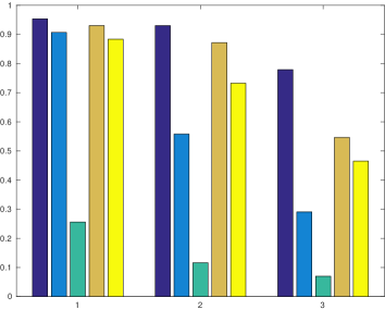
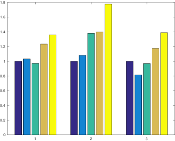
Figure 3.1: Relative reliabilities and iteration numbers

         

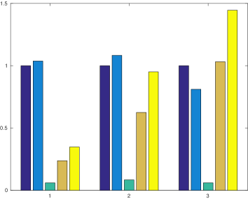
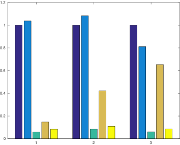
Figure 3.2: Relative energy savings for the evaluations of $f$ and $g$

The following conclusions follow from Table 3.3 and Figures 3.1-3.2.

1. For moderate final accuracy requirements ($\epsilon=10^{-3}$ or $10^{-5}$), the inexact variants iLMQN-a and iLMQN-b perform well: they provide very acceptable robustness compared to the exact method and, most importantly here, yield very significant savings in costs, both for the gradient and the objective function, at the price of a reasonable increase in the number of iterations.

2. The iLMQN-a variant appears to dominate the iLMQN-b in robustness and savings in the evaluation of the objective function. iLMQN-b nevertheless shows significantly larger savings in the gradient’s evaluation costs, but worse performance for the evaluation of the objective function.

3. When the final accuracy is thigher ($\epsilon=10^{-7}$), the inexact methods seem to loose their edge. Not only they become less robust (especially iLMQN-b), but the gains in function evaluation costs disappear (while those in gradient evaluation costs remain significant for the problems the methods are able to solve). A closer examination of the detailed numerical results indicates that, unsurprisingly, inexact methods mostly fail on ill-conditioned problems (e.g. brownbs, powellbs, meyer3, osborneb).

4. The comparison of iLMQN-a and even iLMQN-b with LMQN-s and LMQN-h clearly favours the new methods both in robustness and gains obtained, showing that purpose-designed algorithms outperform simple-minded approaches in this context.

Summarizing, the iLMQN-a multi-precision algorithm appears, in our experiments, to produce significant savings in function’s and gradient’s evaluation costs when the final accuracy requirement and/or the problem conditioning is moderate. Using the iLMQN-b variant may produce, on the problems where it succeeds, larger gains in gradient’s evaluation cost at the price of more costly function evaluations.

4 Conclusions and Perspectives

We have provided an improved provably convergent variant of the trust-region method using dynamic accuracy and have shown that, when considered in the context high performance computing and multiprecision arithmetic, this variant has the potential to bring significant savings in objective function’s and gradient’s evaluation cost.

In the deep learning context, computation in reduced accuracy has already attracted a lot of attention (see [34] and references therein, for instance), but the process, for now, lacks adaptive mechanisms and formal accuracy guarantees. Our approach can be seen as a step towards providing them, and the implemenation of our ideas in practical deep learning frameworks is the object of ongoing research.

Despite the encouraging results reported in this note, the authors are of course aware that the numerical experiments discussed here are limited in size and scope and that the suggested conclusions need further assessment. In particular, it may be of interest to compare inexact trust-region algorithms with inexact regularization methods [4], especially if not only first-order but also second-order critical points are sought.

Appendix: Complexity Theory for the TR1DA Algorithm

For the sake of accuracy and completeness, we now provide details of the first-order worst-case complexity analyis summarized at the end of Section 2. As indicated there, the following development can be seen as a combination of the arguments proposed by [16] for the convergence theory of trust-region methods with inexact gradients (pp. 280sq) and dynamic accuracy (pp. 400).

We assume that

AS.1:

The objective function $f$ is twice continuously differentiable in $\hbox{I\hskip-2.0ptR}^{n}$ and there exist a constant $\kappa_{\nabla}\geq 0$ such that $\|\nabla_{x}^{2}f(x)\|\leq\kappa_{\nabla}$ for all $x\in\hbox{I\hskip-2.0ptR}^{n}$.

AS.2:

There exists a constant $\kappa_{H}\geq 0$ such that $\|H_{k}\|\leq\kappa_{H}$ for all $k\geq 0$.

AS.3

There exists a constant $\kappa_{\rm low}$ such that $f(x)\geq\kappa_{\rm low}$ for all $x\in\hbox{I\hskip-2.0ptR}^{n}$.

Lemma A.1

Suppose AS.1 and AS.2 hold. Then, for each $k\geq 0$, $$|f(x_{k}+s_{k})-m(x_{k},s_{k})|\leq|f_{k}-f(x_{k})|+\kappa_{g}\|\overline{g}(x_{k},\omega_{g,k})\|\Delta_{k}+\kappa_{H\nabla}\Delta_{k}^{2}.$$ (A.1) for $\kappa_{H\nabla}=1+\max[\kappa_{H},\kappa_{\nabla}]$.

• Proof.   (See [16, Theorem 8.4.2].) The definition (2.8), (2.6), the mean-value theorem, the Cauchy-Schwarz inequality and AS.1 give that, for some $\xi_{k}$ in the segment $[x_{k},x_{k}+s_{k}]$,

  $$\begin{array}[]{lcl}|f(x_{k}+s_{k})-m(x_{k},s_{k})|&\leq&|f_{k}-f(x_{k})|+|s_{k}^{T}(\nabla_{x}^{1}f(x_{k})-\overline{g}(x_{k},\omega_{g,k})|\\[6.45831pt] &&\;\;\;\;\;\;\;\;+{\scriptstyle\frac{1}{2}}|s_{k}^{T}\nabla_{x}^{2}f(\xi_{k})s_{k}|+{\scriptstyle\frac{1}{2}}|s_{k}^{T}H_{k}s_{k}|\\[6.45831pt] &\leq&|f_{k}-f(x_{k})|+\kappa_{g}\|\overline{g}(x_{k},\omega_{g,k})\|\,\|s_{k}\|+{\scriptstyle\frac{1}{2}}(\kappa_{H}+\kappa_{\nabla})\|s_{k}\|^{2}\end{array}$$

  and (A.1) follows from the the Cauchy-Schwarz inequality and the inequality $\|s_{k}\|\leq\Delta_{k}$. $\Box$

Lemma A.2

We have that, for all $k\geq 0$, $$\max\left[|f_{k}-f(x_{k})|,|f_{k}^{+}-f(x_{k}+s_{k})|\right]\leq\eta_{0}\left[m(x_{k},0)-m(x_{k},s_{k})\right]$$ (A.2) and $$\rho_{k}\geq\eta_{1}\;\;\mbox{ implies that }\;\;\frac{f(x_{k})-f(x_{k}+s_{k})}{m(x_{k},0)-m(x_{k},s_{k})}\geq\eta_{1}-2\eta_{0}>0.$$ (A.3)

• Proof.   (See [16, p. 401].) The mechanism of the TR1DA algorithm ensures that (A.2) holds. Hence,

  $$\frac{\left[f_{k}-f(x_{k})\right]+\left[|f_{k}^{+}-f(x_{k}+s_{k})\right]}{m(x_{k},0)-m(x_{k},s_{k})}\leq 2\eta_{0}.$$

  As a consequence, for iterations where $\rho_{k}\geq\eta_{1}$,

  $$\rho_{k}=\frac{f_{k}-f_{k}^{+}}{m(x_{k},0)-m(x_{k},s_{k})}=\frac{f(x_{k})-f(x_{k}+s_{k})}{m(x_{k},0)-m(x_{k},s_{k})}+\frac{\left[f_{k}-f(x_{k})\right]+\left[|f_{k}^{+}-f(x_{k}+s_{k})\right]}{m(x_{k},0)-m(x_{k},s_{k})}$$

  and (A.3) must hold. $\Box$

This result implies, in particular, that the sequence $\{f(x_{k})\}_{k\geq 0}$ is non-increasing, and the TR1DA algorithm is therefore monotone on the exact function $f$.

Lemma A.3

Suppose AS.1 and AS.2 hold, and that $\overline{g}(x_{k},\omega_{g,k})\neq 0$. Then $$\Delta_{k}\leq\frac{\|\overline{g}(x_{k},\omega_{g,k})\|}{2\kappa_{H\nabla}}\Big{[}{\scriptstyle\frac{1}{2}}(1-\eta_{1})-\eta_{0}-\kappa_{g}\Big{]}\;\;\mbox{implies that}\;\;\Delta_{k+1}\geq\Delta_{k}.$$ (A.4)

• Proof.   (See [16, Theorem 8.4.3].) Since (2.5) implies that ${\scriptstyle\frac{1}{2}}(1-\eta_{1})-\eta_{0}-\kappa_{g}\in(0,1)$ the first part of (A.4) then gives that $\Delta_{k}<\|\overline{g}(x_{k},\omega_{g,k})\|/\kappa_{H\nabla}$. Hence the inequality $1+\|H_{k}\|\leq\kappa_{H\nabla}$ and (2.9) yield that

  $$m(x_{k},0)-m(x_{k},s_{k})\geq{\scriptstyle\frac{1}{2}}\|\overline{g}(x_{k},\omega_{g,k})\|\min\left[\frac{\|\overline{g}(x_{k},\omega_{g,k})\|}{\kappa_{H\nabla}},\Delta_{k}\right]={\scriptstyle\frac{1}{2}}\|\overline{g}(x_{k},\omega_{g,k})\|\,\Delta_{k}.$$

  As a consequence, we may use (2.11), the Cauchy-Schwarz inequality, (A.2) (twice), (A.1), the inequality $\kappa_{H\nabla}\geq 1$ and the first part of (A.4) to deduce that, for all $k\geq 0$,

  $$\begin{array}[]{lcl}|\rho_{k}-1|&=&\frac{\displaystyle|f_{k}^{+}-m(x_{k},s_{k})|}{\displaystyle m(x_{k},0)-m(x_{k},s_{k})}\\[6.45831pt] &\leq&\frac{\displaystyle|f_{k}^{+}-f(x_{k}+s_{k})|+|f(x_{k}+s_{k})-m(x_{k},s_{k})|}{\displaystyle m(x_{k},0)-m(x_{k},s_{k})}\\[6.45831pt] &\leq&2\eta_{0}+\frac{\displaystyle\kappa_{g}\|\overline{g}(x_{k},\omega_{g,k})\|\Delta_{k}+\kappa_{H\nabla}\Delta_{k}^{2}}{\displaystyle{\scriptstyle\frac{1}{2}}\|\overline{g}(x_{k},\omega_{g,k})\|\,\Delta_{k}}\\[6.45831pt] &\leq&2\eta_{0}+2\kappa_{g}+2\kappa_{H\nabla}\frac{\displaystyle\Delta_{k}}{\displaystyle\|\overline{g}(x_{k},\omega_{g,k})\|}\\[6.45831pt] &\leq&1-\eta_{2}.\end{array}$$

  Thus $\rho_{k}\geq\eta_{2}$ and (2.12) ensures the second part of (A.4). $\Box$

Lemma A.4

Suppose that AS.1 and AS.2 hold. Then, before termination, $$\Delta_{k}\geq\min\left[\Delta_{0},\theta\epsilon\right]\;\;\mbox{ where }\;\;0<\theta\stackrel{{\scriptstyle\rm def}}{{=}}\frac{\gamma_{1}\big{[}{\scriptstyle\frac{1}{2}}(1-\eta_{1})-\eta_{0}-\kappa_{g}\big{]}}{\kappa_{H\nabla}(1+\kappa_{g})}<\frac{1}{\kappa_{H\nabla}(1+\kappa_{g})}.$$ (A.5)

• Proof.   (See [16, Theorem 8.4.4].) Before termination, we must have that

  $$\|\overline{g}(x_{k},\omega_{g,k})\|\geq\frac{\epsilon}{1+\kappa_{g}}.$$ (A.6)

  Suppose that iteration $k$ is the first iteration such that

  $$\Delta_{k+1}\leq\frac{\gamma_{1}\epsilon}{\kappa_{H\nabla}(1+\kappa_{g})}\big{[}{\scriptstyle\frac{1}{2}}(1-\eta_{1})-\eta_{0}-\kappa_{g}\big{]}.$$ (A.7)

  Then the update (2.12) implies that

  $$\Delta_{k}\leq\frac{\epsilon}{\kappa_{H\nabla}(1+\kappa_{g})}\big{[}{\scriptstyle\frac{1}{2}}(1-\eta_{1})-\eta_{0}-\kappa_{g}\big{]}\leq\frac{\|\overline{g}(x_{k},\omega_{g,k})\|}{\kappa_{H\nabla}}\big{[}{\scriptstyle\frac{1}{2}}(1-\eta_{1})-\eta_{0}-\kappa_{g}\big{]}$$

  where we have used (A.6) to deduce the last inequality. But this bound and (A.4) imply that $\Delta_{k+1}\geq\Delta_{k}$, which is impossible since $\Delta_{k}$ is reduced at iteration $k$. Hence no $k$ exists such that (A.7) holds and the desired conclusion follows. $\Box$

Lemma A.5

For each $k\geq 0$, define $${\cal S}_{k}\stackrel{{\scriptstyle\rm def}}{{=}}\{j\in\{0,\ldots,k\}\mid\rho_{j}\geq\eta_{1}\}\;\;\mbox{ and }\;\;{\cal U}_{k}\stackrel{{\scriptstyle\rm def}}{{=}}\{0,\ldots,k\}\setminus{\cal S}_{k}.$$ (A.8) the index sets of “successful” and “unsuccessful” iterations, respectively. Then $$k\leq|{\cal S}_{k}|\left(1-\frac{\log\gamma_{3}}{\log\gamma_{2}}\right)+\frac{1}{|\log\gamma_{2}|}\log\left(\frac{\Delta_{0}}{\theta\epsilon}\right).$$ (A.9)

• Proof.   Observe that (2.12) implies that

  $$\Delta_{j+1}\leq\gamma_{3}\Delta_{j}\;\;\mbox{ for }\;\;j\in{\cal S}_{k}$$

  and that

  $$\Delta_{j+1}\leq\gamma_{2}\Delta_{j}\;\;\mbox{ for }\;\;j\in{\cal U}_{k}.$$

  Combining these two inequalities, we obtain from (A.5) that

  $$\min\big{[}\Delta_{0},\theta\epsilon\Big{]}\leq\Delta_{k}\leq\Delta_{0}\gamma_{3}^{|S_{k}|}\gamma_{2}^{|U_{k}|}$$

  Dividing by $\Delta_{0}$, taking logarithms and recalling that $\gamma_{2}\in(0,1)$, we get

  $$|{\cal U}_{k}|\leq-|{\cal S}_{k}|\frac{\log\gamma_{3}}{\log\gamma_{2}}-\frac{1}{\log\gamma_{2}}\log\left(\frac{\Delta_{0}}{\theta\epsilon}\right).$$

  Hence (A.9) follows since $k=|{\cal S}_{k}|+|{\cal U}_{k}|$. $\Box$

Theorem A.6

Suppose that AS.1–AS.3 hold. Suppose also that $\Delta_{0}\geq\theta\epsilon$, where $\theta$ is defined in (A.5). Then the TR1DA algorithm produces an iterate $x_{k}$ such that $\|\nabla_{x}^{1}f(x_{k})\|\leq\epsilon$ in at most $$\tau_{\cal S}\stackrel{{\scriptstyle\rm def}}{{=}}\frac{2(f(x_{0})-\kappa_{\rm low})(1+\kappa_{g})}{(\eta_{1}-2\eta_{0})\theta}\cdot\frac{1}{\epsilon^{2}}$$ (A.10) successful iterations, at most $$\tau_{\rm tot}\stackrel{{\scriptstyle\rm def}}{{=}}\tau_{S}\left(1-\frac{\log\gamma_{3}}{\log\gamma_{2}}\right)+\frac{1}{|\log\gamma_{2}|}\log\left(\frac{\Delta_{0}}{\theta\epsilon}\right)$$ (A.11) iterations in total, at most $\tau_{\rm tot}$ (approximate) evaluations of the gradient satisfying (2.6), and at most $2\tau_{\rm tot}$ (approximate) evaluations of the objective function satisfying (2.2).

• Proof.    As in the previous proof, (A.6) must hold before termination. Using AS.3, (A.8), (A.3), (2.9), (A.6), the assumption that $\Delta_{0}\geq\theta\epsilon$ and (A.5), we obtain that, for an arbitrary $k\geq 0$ before termination,

  $$\begin{array}[]{lcl}f(x_{0})-\kappa_{\rm low}&\geq&\displaystyle\sum_{j\in{\cal S}_{k}}\left[f(x_{j})-f(x_{j+1})\right]\\[6.45831pt] &\geq&(\eta_{1}-2\eta_{0})\displaystyle\sum_{j\in{\cal S}_{k}}\left[m(x_{j},0)-m(x_{j},s_{j})\right]\\[6.45831pt] &\geq&{\scriptstyle\frac{1}{2}}(\eta_{1}-2\eta_{0})\displaystyle\sum_{j\in{\cal S}_{k}}\|\overline{g}(x_{j},\omega_{g,j})\|\min\left[\frac{\displaystyle\|\overline{g}(x_{j},\omega_{g,j})\|}{\displaystyle 1+\|H_{j}\|},\Delta_{j}\right]\\[6.45831pt] &\geq&{\scriptstyle\frac{1}{2}}|{\cal S}_{k}|(\eta_{1}-2\eta_{0})\frac{\displaystyle\epsilon}{\displaystyle 1+\kappa_{g}}\min\left[\frac{\displaystyle\epsilon}{\displaystyle\kappa_{H\nabla}(1+\kappa_{g})},\min\Big{[}\Delta_{0},\theta\epsilon\Big{]}\right]\\[6.45831pt] &=&|{\cal S}_{k}|\,\frac{\displaystyle(\eta_{1}-2\eta_{0})}{\displaystyle 2(1+\kappa_{g})}\min\left[\frac{\displaystyle 1}{\displaystyle\kappa_{H\nabla}(1+\kappa_{g})},\theta\right]\,\epsilon^{2}\\[6.45831pt] &=&|{\cal S}_{k}|\,\frac{\displaystyle(\eta_{1}-2\eta_{0})\theta}{\displaystyle 2(1+\kappa_{g})}\,\epsilon^{2}\end{array}$$

  and therefore

  $$|{\cal S}_{k}|\leq\frac{2(f(x_{0})-\kappa_{\rm low})(1+\kappa_{g})}{(\eta_{1}-2\eta_{0})\theta}\cdot\frac{1}{\epsilon^{2}}\stackrel{{\scriptstyle\rm def}}{{=}}\frac{\tau_{\cal S}}{\epsilon^{2}}.$$

  As a consequence $\|\overline{g}(x_{k},\omega_{g,k})\|<\epsilon/(1+\kappa_{g})$ after at most $\tau_{S}\epsilon^{-2}$ successful iterations and the algorithm terminates. The relation (2.13) then ensures that $\|\nabla_{x}^{1}f(x_{k})\|<\epsilon$, yielding (A.10). We may now use (A.9) and the mechanism of the algorithm to complete the proof. $\Box$

Given that $\epsilon\in(0,1]$, we immediately note that

$$\tau_{\cal S}={\cal O}(\epsilon^{-2})\;\;\mbox{and}\;\;\tau_{\rm tot}={\cal O}(\epsilon^{-2}).$$

Moreover, the proof of Theorem A.6 implies that these complexity bounds improve from ${\cal O}(\epsilon^{-2})$ to ${\cal O}(\epsilon^{-1})$ if $\epsilon$ is so large or $\Delta_{0}$ so small to yield $\Delta_{0}<\theta\epsilon$.

We conclude this brief complexity theory by noting that the domain in which AS.1 is assumed to hold can be restricted to the “tree of iterates” $\cup_{k\geq 0}[x_{k},x_{k}+s_{k}]$ without altering our results. This can be useful if an upper bound $\bar{\Delta}$ is imposed on the step’s length, in which case the monotonicty of the algorithm ensures that the tree of iterates remains in the set

$$\{y\in\hbox{I\hskip-2.0ptR}^{n}\,|\,y=x+s\;\;\mbox{with}\;\;f(x)\leq f(x_{0})\;\;\mbox{and}\;\;\|s\|\leq\bar{\Delta}\}.$$

While it can be difficult to verify AS.1 on the (a priori unpredictable) tree of iterates, verifying it on the above set is much easier.

References

- [1] M. Baboulin, A. Buttari, J. Dongarra, J. Kurzak, J. Langou, P. Luszczek, and S. Tomov. Accelerating scientific computations with mixed precision algorithms. Comput. Phys. Commun., 180:2526–2533, 2009.
- [2] S. Bellavia, S. Gratton, and E. Riccietti. A Levenberg-Marquardt method for large nonlinear least-squares problems with dynamic accuracy in functions and gradients. Numerische Mathematik, 140:791–825, 2018.
- [3] S. Bellavia, G. Gurioli, and B. Morini. Theoretical study of an adaptive cubic regularization method with dynamic inexact Hessian information. arXiv:1808.06239, 2018.
- [4] S. Bellavia, G. Gurioli, B. Morini, and Ph. L. Toint. Deterministic and stochastic inexact regularization algorithms for nonconvex optimization with optimal complexity. arXiv:1811.03831, 2018.
- [5] E. Bergou, Y. Diouane, V. Kungurtsev, and C. W. Royer. A subsampling line-search method with second-order results. arXiv:1810.07211, 2018.
- [6] J. Blanchet, C. Cartis, M. Menickelly, and K. Scheinberg. Convergence rate analysis of a stochastic trust region method via supermartingales. arXiv:1609.07428v3, 2018.
- [7] A.A. Brown and M. Bartholomew-Biggs. Some effective methods for unconstrained optimization based on the solution of ordinary differential equations. Technical Report Technical Report 178, Hatfield Polytechnic, Hatfield, UK, 1987.
- [8] A. G. Buckley. Test functions for unconstrained minimization. Technical Report CS-3, Computing Science Division, Dalhousie University, Dalhousie, Canada, 1989.
- [9] R. G. Carter. A worst-case example using linesearch methods for numerical optimization with inexact gradient evaluations. Technical Report MCS-P283-1291, Argonne National Laboratory, Argonne, USA, 1991.
- [10] R. G. Carter. Numerical experience with a class of algorithms for nonlinear optimization using inexact function and gradient information. SIAM Journal on Scientific and Statistical Computing, 14(2):368–388, 1993.
- [11] C. Cartis, N. I. M. Gould, and Ph. L. Toint. Worst-case evaluation complexity and optimality of second-order methods for nonconvex smooth optimization. To appear in the Proceedings of the 2018 International Conference of Mathematicians (ICM 2018), Rio de Janeiro, 2018.
- [12] C. Cartis and K. Scheinberg. Global convergence rate analysis of unconstrained optimization methods based on probabilistic models. Mathematical Programming, Series A, 159(2):337–375, 2018.
- [13] X. Chen, B. Jiang, T. Lin, and S. Zhang. On adaptive cubic regularization Newton’s methods for convex optimization via random sampling. arXiv:1802.05426, 2018.
- [14] A. R. Conn, N. I. M. Gould, M. Lescrenier, and Ph. L. Toint. Performance of a multifrontal scheme for partially separable optimization. In S. Gomez and J. P. Hennart, editors, Advances in Optimization and Numerical Analysis, Proceedings of the Sixth Workshop on Optimization and Numerical Analysis, Oaxaca, Mexico, volume 275, pages 79–96, Dordrecht, The Netherlands, 1994. Kluwer Academic Publishers.
- [15] A. R. Conn, N. I. M. Gould, and Ph. L. Toint. LANCELOT: a Fortran package for large-scale nonlinear optimization (Release A). Number 17 in Springer Series in Computational Mathematics. Springer Verlag, Heidelberg, Berlin, New York, 1992.
- [16] A. R. Conn, N. I. M. Gould, and Ph. L. Toint. Trust-Region Methods. MPS-SIAM Series on Optimization. SIAM, Philadelphia, USA, 2000.
- [17] L. C. W. Dixon and Z. Maany. A family of test problems with sparse Hessian for unconstrained optimization. Technical Report 206, Numerical Optimization Center, Hatfield Polytechnic, Hatfield, UK, 1988.
- [18] C. Elster and A. Neumaier. A method of trust region type for minimizing noisy functions. Computing, 58(1):31–46, 1997.
- [19] S. Galal and M. Horowitz. Energy-efficient floating-point unit design. IEEE Transactions on Computers, 60(7), 2011.
- [20] N. I. M. Gould, D. Orban, and Ph. L. Toint. CUTEst: a constrained and unconstrained testing environment with safe threads for mathematical optimization. Computational Optimization and Applications, 60(3):545–557, 2015.
- [21] A. Griewank and Ph. L. Toint. Partitioned variable metric updates for large structured optimization problems. Numerische Mathematik, 39:119–137, 1982.
- [22] N. J. Higham. The rise of multiprecision computations. Talk at SAMSI 2017, April 2017. https://bit.ly/higham-samsi17.
- [23] L. Kugler. Is “good enough” computing good enough? Commun. ACM, 58:12–14, 2015.
- [24] S. Leyffer, S. Wild, M. Fagan, M. Snir, K. Palem, K. Yoshii, and H. Finkel. Moore with less – leapgrogging Moore’s law with inexactness for supercomputing. arXiv:1610.02606v2, 2016. (to appear in Proceedings of PMES 2018: 3rd International Workshop on Post Moore’s Era Supercomputing).
- [25] G. Li. The secant/finite difference algorithm for solving sparse nonlinear systems of equations. SIAM Journal on Numerical Analysis, 25(5):1181–1196, 1988.
- [26] S. Matsuoka. private communication, March 2018.
- [27] J. J. Moré, B. S. Garbow, and K. E. Hillstrom. Testing unconstrained optimization software. ACM Transactions on Mathematical Software, 7(1):17–41, 1981.
- [28] J. Nocedal and S. J. Wright. Numerical Optimization. Series in Operations Research. Springer Verlag, Heidelberg, Berlin, New York, 1999.
- [29] K. V. Palem. Inexactness and a future of computing. Phil. Trans. R. Soc. A, 372(20130281), 2014.
- [30] G. Poenisch and H. Schwetlick. Computing turning points of curves implicitly defined by nonlinear equations depending on a parameter. Computing, 20:101–121, 1981.
- [31] J. Pu, S. Galal, X. Yang, O. Shacham, and M. Horowitz. FPMax: a 106GFLOPS/W at 217GFLOPS/mm2 single-precision FPU, and a 43.7 GFLOPS/W at 74.6 GFLOPS/mm2 double-precision FPU, in 28nm UTBB FDSOI. Hardware Architecture, 2016.
- [32] J.W. Schmidt and K. Vetters. Albeitungsfreie verfahren fur nichtlineare optimierungsproblem. Numerische Mathematik, 15:263–282, 1970.
- [33] E. Spedicato. Computational experience with quasi-Newton algorithms for minimization problems of moderately large size. Technical Report CISE-N-175, CISE Documentation Service, Segrate, Milano, 1975.
- [34] N. Wang, J. Choi, D. Brand, C.-Y. Chen, and K. Gopalakrishnan. Training deep neural networks with 8-bit floating point numbers. In 32nd Conference on Neural Information Processing Systems, 2018.
- [35] P. Xu, F. Roosta-Khorasani, and M. W. Mahoney. Newton-type methods for non-convex optimization under inexact Hessian information. arXiv:1708.07164v3, 2017.