Cyclotron lines in highly magnetized neutron stars
Cyclotron lines, also called cyclotron resonant scattering features (CRSF) are spectral features, generally appearing in absorption, in the X-ray spectra of objects containing highly magnetized neutron stars, allowing the direct measurement of the magnetic field strength in these objects. Cyclotron features are thought to be due to resonant scattering of photons by electrons in the strong magnetic fields. The main content of this contribution focusses on electron cyclotron lines as found in accreting X-ray binary pulsars (XRBP) with magnetic fields on the order of several Gauss. Also, possible proton cyclotron lines from single neutron stars with even stronger magnetic fields are briefly discussed. With regard to electron cyclotron lines, we present an updated list of XRBPs that show evidence of such absorption lines. The first such line was discovered in a 1976 balloon observation of the accreting binary pulsar Hercules X-1, it is considered to be the first direct measurement of the magnetic field of a neutron star. As of today (mid 2018), we list 36 XRBPs showing evidence of one ore more electron cyclotron absorption line(s). A few have been measured only once and must be confirmed (several more objects are listed as candidates). In addition to the Tables of objects, we summarize the evidence of variability of the cyclotron line as a function of various parameters (especially pulse phase, luminosity and time), and add a discussion of the different observed phenomena and associated attempts of theoretical modeling. We also discuss our understanding of the underlying physics of accretion onto highly magnetized neutron stars. For proton cyclotron lines, we present tables with seven neutron stars and discuss their nature and the physics in these objects.
Key Words.:
magnetic fields, neutron stars, – radiation mechanisms, cyclotron scattering features – accretion, accretion columns – binaries: eclipsing – stars: Her X-1 – X-rays: general – X-rays: stars1 Introduction
In this contribution we review the status of cyclotron line research in the X-ray range, preferentially from an observational point of view, together with the related theoretical background, and some recent progress in modeling the relevant physics. Highly magnetized accreting neutron stars (NSs) in binary systems generally reveal themselves as X-ray pulsars. A substantial fraction of those objects show line-like features in their high energy X-ray spectra, mostly in absorption at energies from 10 keV to 100 keV, called cyclotron lines or cyclotron resonant scattering features (CRSFs). The following introductory statements are for objects with electron cyclotron lines (we will come to proton cyclotron line objects below). Such lines are generated close to the magnetic poles of accreting neutron stars in the hot, highly magnetized plasma where the kinetic energy of the in-falling material is converted to heat and radiation. Electrons assume discrete energies with respect to their movement perpendicular to the magnetic field, so called Landau levels. Resonant scattering of photons on these electrons then leads to scattering of photons at the resonance energy and to the generation of resonance features (in absorption) in the X-ray spectrum. The fundamental energy quantum corresponds to the energy difference between adjacent Landau levels, given by , where is the gyro frequency, is the electron charge, B is the magnetic field in the scattering region, is the mass of the electron, and is the speed of light. The Landau levels (to first order equidistant) are linearly related to the strength of the magnetic field. The observation of such features then allows for the measurement of the magnetic field strength. The following centroid line energies are expected:
| (1) |
where is the magnetic field strength in units of Gauss, z is the gravitational redshift due to the NS mass and n is the number of Landau levels involved: e.g., n = 1 is the case of a scattering from the ground level to the first excited Landau level and the resulting line is called the fundamental line. In the case of n = 2 (or higher) the lines are called harmonics.
The same physics is valid for other charged particles, for example protons, for which the difference between Landau levels is smaller by a factor of 1836 (the ratio of the proton to electron mass). Such lines are thought to be observed from isolated, thermally radiating neutron stars in the range 0.1 keV to a few keV. For the proton cyclotron lines to appear in the X-ray range, the magnetic field must typically be two orders of magnitude stronger than for electron cyclotron lines.
Cyclotron line research with accreting X-ray binaries (or isolated neutron stars) has become a field of its own within X-ray astronomy. It is a vibrant field, in both theoretical and in observational work, dealing not only with the detection of new lines, but also with various recently discovered properties of these lines, such as the dependence of the line energy, width and depth on X-ray luminosity and its long-term evolution with time. Cyclotron lines are an important diagnostic tool to investigate the physics of accretion onto the magnetic poles of highly magnetized neutron stars.
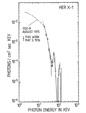
Here we give a brief history of the beginning of cyclotron line research and its evolution up to the present. The discovery of cyclotron lines in 1976 in the X-ray spectrum of Her X-1 (Trümper et al., 1977, 1978) (see Fig. 1) was not the result of a targeted search, but came as a surprise. A joint group of the Astronomical Institute Tübingen (AIT) and the Max Planck Institute for Extraterrestrial Physics (MPE) had flown a hard X-ray balloon payload (“Balloon HEXE”) on 2-3 May 1976, observing Her X-1 and Cygnus X-1 at energies from 20 keV to 200 keV. While the AIT group concentrated on the analysis of the energy dependent pulse profiles (Kendziorra et al., 1977), their colleagues at MPE dealt with the energy spectrum. They found an unexpected shoulder-like deviation from the steep total energy spectrum around 50 keV which looked like a resonance feature. Detailed investigations showed that the feature was present in the pulsed spectrum and absent in the Cygnus X-1 spectrum taken on the same balloon flight, excluding the possibility of a spurious origin. Because of its high energy and intensity it could be attributed only to the electron cyclotron resonance.
This discovery was first reported in a very late talk – proposed and accepted during the meeting – at the Eighth Texas Symposium on Relativistic Astrophysics on 16 December 1976 (Trümper et al., 1977), and became a highlight of that meeting. An extended version that appeared later (Trümper et al., 1978) has become the standard reference for the discovery which revealed a new phenomenon in X-ray astronomy and provided the first direct measurement of a neutron star magnetic field, opening a new avenue of research in the field. The limited spectral resolution of the Balloon-HEXE did not allow us to distinguish between an emission or absorption line (Trümper et al., 1978). For the answer to this question we had to await radiative transfer calculations in strong magnetic fields. For that the pioneering work on the magnetic photon-electron cross sections was important (Lodenquai et al., 1974; Gnedin & Sunyaev, 1974). The latter work – based on the assumption of a (Thomson) optically thin radiation source – also predicted that at the cyclotron a resonance emission line would occur (see also Basko & Sunyaev 1975).
The discovery of the Her X-1 cyclotron lines spurred a burst of early theoretical papers on the radiative transfer in strongly magnetized plasmas. Some of them provided support for an emission line interpretation of the feature (e.g., Daugherty & Ventura 1977; Meszaros 1978; Yahel 1979b, a; Wasserman & Salpeter 1980; Melrose & Zhelezniyakov 1981). The first support for an absorption line interpretation came from a talk by Andy Fabian at the first international workshop on cyclotron lines, organized by the Max-Planck-Institut für extraterrestrische Physik (MPE) in fall 1978. His argument was: the radiating high temperature plasma would be optically thick. In the cyclotron resonance region the reflectivity would be high and according to the Kirchhoff law the emissivity would be low (Fabian 1978, unpublished). Other important early theoretical papers followed (e.g., Bonazzola et al. 1979; Ventura et al. 1979; Bussard 1980; Kirk & Meszaros 1980; Langer et al. 1980; Nagel 1980; Yahel 1980a, b; Pravdo & Bussard 1981; Nagel 1981a, b; Meszaros et al. 1983). All these and many following works led to the current view that these lines are seen “in absorption”. This was also observationally verified for Her X-1 in 1996 through data from Mir-HEXE (Staubert, 2003). The first significant confirmation of the cyclotron line in Her X-1 came in 1980 on the basis of HEAO-1/A4 observations (Gruber et al., 1980). The same experiment discovered a cyclotron line at 20 keV in the source 4U 0115+63 (Wheaton et al., 1979). A re-examination of the data uncovered the existence of two lines at 11.5 and 23 keV which were interpreted as the fundamental and harmonic electron cyclotron resonances seen in absorption (White et al., 1983). Later observations of the source found it to show three (Heindl et al., 1999), four (Santangelo et al., 1999), and finally up to five lines in total (Heindl et al., 2004).
In many accreting X-ray binary pulsars (XRBPs) the centroid energy of cyclotron lines is seen to vary. The first variations seen were variations of with pulse phase (e.g., Voges et al. 1982; Soong et al. 1990; Vasco et al. 2013), and are attributed to a varying viewing angle to the scattering region. A negative correlation between and the X-ray luminosity was reported during high luminosity outbursts of two X-ray transients: V 0332+53 and 4U 0115+63 (Makishima et al., 1990a; Mihara, 1995). Today we consider this to be real only in V 0332+53 (see Sect. 4.2). It was again in Her X-1 that two more variability phenomena were first detected: firstly, a positive correlation of with the X-ray luminosity (Staubert et al., 2007) and secondly, a long-term decay of with time (Staubert et al., 2014) (revealing a 5 keV reduction over the last 20 years). Today we know a total of seven objects showing the same positive correlation (see Sect. 4.2), and one more example for a long-term decay (Vela X-1, La Parola et al. 2016) (Sect. 4.4).
In the last 40 years the number of known electron cyclotron sources has increased to 36 (see Table LABEL:tab:collection) due to investigations with many X-ray observatories like Ginga, MIR-HEXE, RXTE, BeppoSAX, INTEGRAL, Suzaku, and NuSTAR. For previous reviews about cyclotron line sources, see for example, Coburn et al. (2002); Staubert (2003); Heindl et al. (2004); Terada et al. (2007); Wilms (2012); Caballero & Wilms (2012); Revnivtsev & Mereghetti (2016); Maitra (2017). Lists of CRSF sources can also be found at the webpages of Dr. Remeis-Sternwarte, Bamberg111http://www.sternwarte.uni-erlangen.de/wiki/doku.php?id=xrp:start and the Istituto Astrrofisica Spaziale, Bologna222http://www.iasfbo.inaf.it/~mauro/pulsar_list.html. Recent theoretical work has followed two lines: analytical calculations (Nishimura, 2008, 2011, 2013, 2014) or making use of Monte Carlo techniques (Araya & Harding, 1999; Araya-Góchez & Harding, 2000; Schönherr et al., 2007; Schwarm et al., 2017b, a). In addition, evidence for the detection of proton cyclotron lines in the thermal spectra of isolated neutron stars was provided by Chandra and XMM-Newton (Haberl, 2007) (see Tables 22 and 23). In this paper we review the status of cyclotron line research by summarizing the current knowledge about cyclotron line sources (both electron- and proton-cyclotron line sources) and the state of our understanding of the the details of the underlying physics.
This paper is structured as follows: in Sect. 2 we present a series of tables, which contain detailed information about all objects known to us which show conclusive evidence for the existence of electron cyclotron lines (together with appropriate references), plus several uncertain candidate objects. In Sect. 3 we discuss issues of spectral fitting, including a list of popular functions for the modeling of the continuum and the cyclotron lines, as well as systematic differences that must be taken into consideration when different results from the literature are to be compared. Sect. 4 discusses observed variations of measured cyclotron line energies (as summarized in Table 6): we find that the line energy can vary with pulse phase, with luminosity (both positive and negative), with time and (in Her X-1) with phase of the super-orbital period. The width and depth of the cyclotron line(s) can also vary systematically with luminosity. It is also found that the spectral hardness of the continuum can vary with X-ray luminosity, in close correlation with variations of the cyclotron line energy. Sect. 4.4 we review the evidence for variations of the cyclotron line energy on medium to long timescales. In Sect. 4.5 the current knowledge about correlations between the various spectral parameters is discussed, and in Sect. 4.6 we discuss a few individual sources, mostly those that show systematic variations with X-ray luminosity. In Sect. 5 we discuss the relevant physics at work in accreting binary X-ray pulsars: the formation of spectral continua and cyclotron lines and the physics behind their systematic variations. In Sect. 5.2 we briefly refer to theoretical modeling of cyclotron features, by both analytical and Monte Carlo methods. In Sect. 6 three methods of how to estimate the magnetic field strength of neutron stars are discussed and compared. In Sect. 7 we present a statistical analysis, describing the overall mean properties of the discussed objects. Finally, in Sect. 8 we discuss objects thought to show proton cyclotron lines and conclude in Sect. 9 with a short general summary.
2 Collection of cyclotron line sources
This review attempts to summarize the current knowledge of cyclotron line sources – both electron-
and proton-cyclotron line sources. For both types of cyclotron line sources we provide a series of tables
with information about a total of more than 40 objects that we consider to show one (or more) cyclotron
lines in their X-ray spectra. Tables 22 and 23 list seven objects with proton-cyclotron lines.
For electron-cyclotron line objects we present a total of five tables with the following content:
- Table LABEL:tab:collection: 36 objects with confirmed or reasonably secure CRSFs (14 of them still need further confirmation).
The columns are: source name, type of object, pulse period, orbital period, eclipse (yes/no),
cyclotron line energy (or energies), instrument of first detection, confirmations yes/no, references.
- Table 4: 11 objects which we call “candidates”, for which electron-CRSFs
have been claimed, but where sufficient doubts about the reality of the cyclotron line(s) exist or where additional
observations are needed for confirmation (or not).
- Table 5: HEASARC type, position, optical counterpart, its spectral type, masses, distance, references.
- Table 6: Variation of Ecyc with pulse phase and with Lx, variation of spectral hardness
with Lx, references.
- Table 7: Ecyc, width, “strength’,’ and optical depth of cyclotron lines at certain Lx,
references, notes.
3 Spectral fitting
X-ray spectra of XRBPs are of thermal nature. They are formed in a hot plasma ( K) over the NS magnetic poles where infalling matter arrives with half the speed of light at the stellar surface. The emission process is believed to be governed by Comptonization of thermal photons which gain energy by scattering off hot plasma electrons (thermal Comptonization). In addition, bulk motion Comptonization in the fast moving plasma above the deceleration region and cyclotron emission plays an important role (e.g., Becker & Wolff, 2007; Ferrigno et al., 2013). The shape of the spectral continuum formed by Comptonized photons emitted in the breaking plasma at the polar caps of an accreting magnetized NS was first computed in the seminal work of Lyubarskii & Sunyaev (1982). It has been shown that non-saturated Comptonization leads to a power law-like continuum which cuts off at energies , where denotes the electron temperature in the plasma.
The calculations of Lyubarskii & Sunyaev (1982) and the numerical computations performed later provided a physical motivation for the usage of analytic power law functions with exponential cutoff to model the spectral continua of XRBPs. Historically, the following realizations of such functions became most popular and are included in some of the standard spectral fitting packages such as XSPEC333http://heasarc.nasa.gov/xanadu/xspec, Sherpa444http://cxc.harvard.edu/sherpa and ISIS555http://space.mit.edu/asc/isis. The most simple one, with just three free fit parameters, is the so-called cutoffpl model (these names are the same in all mentioned fitting packages):
| (2) |
where is the photon energy and the free fit parameters , and determine the normalization coefficient, the photon index, and the exponential folding energy,666In XSPEC the folding energy for this function is called respectively. We note that this represents a continuously steepening continuum.
The next function has an additional free parameter, the cutoff energy :
| (3) |
In the spectral fitting packages mentioned here, this function is realized as a product of a power law and a multiplicative exponential factor: power lawhighecut. Although this function is generally more flexible due to one more free parameters, it contains a discontinuity of its first derivative (a “break”) at . Since the observed X-ray spectra are generally smooth, an absorption-line like feature appears in the fit residuals when using this model with high quality data. To eliminate this feature, one either includes an artificial narrow absorption line in the model (e.g., Coburn et al., 2002) or substitutes the part of the function around the “break” with a third order polynomial such that no discontinuity in the derivative appears (e.g., Klochkov et al., 2008a). Here the power law is unaffected until the cutoff energy is reached.
Another form of the power law-cutoff function is a power law with a Fermi-Dirac form of the cutoff (Tanaka, 1986):
| (4) |
which has the same number of free parameters as the previous function. This function is not included any more in the current versions of the fitting packages.
Finally, a sum of two power laws with a positive and a negative photon index multiplied by an exponential cutoff is used in the literature (the NPEX model, Mihara, 1995):
| (5) |
In many applications using this model, is set to a value of two in order to represent the Wien portion of the thermal distribution.
In some spectra of XRBPs with high photon statistics, deviations from these simple phenomenological models are seen. In many cases, a wave-like feature in the fit residuals is present between a few and 10–20 keV. It is often referred to as the “10-keV-feature” (e.g., Coburn et al., 2002). The residuals can be flattened by including a broad emission or absorption line component. Although sometimes interpreted as a separate physical component, the 10-keV-feature most probably reflects the limitations of the simple phenomenological models described above.
To model the cyclotron line, one modifies the continuum functions described above by the inclusion of a corresponding multiplicative component. The following three functions are used in most cases to model CRSFs. The most popular one is a multiplicative factor of the form , where the optical depth has a Gaussian profile:
| (6) |
with , , and
being the central optical depth, the centroid energy, and the width of the line.
We note that in the popular XSPEC realization of this function
gabs, is not explicitely used as a fit parameter. Instead, a product
is defined that is often called the “strength” of the line. The physical motivation for the
described line models stems from the formal solution of the transfer equation in the case of
true absorption lines, for example, due to transitions between the atomic levels in stellar atmospheres. The Gaussian
profile forms as a result of the thermal motion of atoms and reflects their Maxwellian distribution. Such a
physical picture cannot be applied to the cyclotron features whose nature is completely different.
The gabs function should thus be considered as a pure
phenomenological model in the case of CRSFs.
The second widely used phenomenological model has been specifically created to model cyclotron features. It is implemented in the XSPEC cyclabs function which, similarly to gabs, provides a multiplicative factor of the form for the continuum (Mihara et al., 1990; Makishima et al., 1990b). In this model, the line profile is determined by a Lorentzian function multiplied by a factor (not a pure Lorentzian, as it is often claimed in the literature). Eq.7 shows the formula used for for the case of two lines, the fundamental at and the first harmonic at .
| (7) |
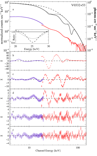
where are the central optical depths of the two lines while characterize their width. One can fix or to zero, if necessary. When using cyclabs, however, one needs to be careful, since the ratio of the true energy centroids may not always be exactly equal to two. Figure 2 gives an example for a spectral fitting of the spectrum of V 0332+53 as observed with RXTE PCA and HEXTE (Pottschmidt et al., 2005) for a Fermi-Dirac continuum model and up to three cyclotron lines, modeled by Gaussian optical depth profiles gabs.
For a substantial fraction of confirmed CRSF sources listed in Table LABEL:tab:collection, multiple cyclotron lines are reported. The harmonic lines correspond to resonant scattering between the ground Landau level and higher excited levels (see Eq.1). The energies of the harmonic lines are thus expected to be multiples of the fundamental line energy. However, the broad and complex profiles of CRSFs, the influence of the spectral continuum shape on the measured line parameters, and various physical effects lead to deviations of the line centroid energies from the harmonic spacing (see e.g., Nishimura, 2008; Schönherr et al., 2007). To model multiple cyclotron lines, it is best to introduce several independent absorption line models (as described above) into the spectral function, leaving the line centroid energies uncoupled.
Soon after the discovery of the cyclotron line in Her X-1, a third possibility was occasionally used. The X-ray continuum was multiplied by a factor , where is a Gaussian function with an amplitude between zero and one (e.g., Voges et al., 1982).
The usage of different spectral functions both for the continuum and for the cyclotron lines poses a natural problem when observational results are to be compared to those that were obtained using different fit functions. It is obvious that the width and the strength/depth of the line are defined in different ways in the models above, such that they cannot be directly compared with each other. Even more challenging is the determination of the centroid energy of the line. In case of a symmetric and sufficiently narrow absorption line, for which variations of the continuum over the energy range affected by the line can be neglected, one naturally expects that the models above would return very similar centroid energies. But, the cyclotron lines are (i) mostly quite broad and (ii) are overlaid on a highly inclined continuum which changes exponentially with energy. Furthermore, real lines can be noticeably asymmetric (e.g., Fürst et al., 2015). The line centroids measured with different spectral functions are therefore systematically different. Specifically, our systematic analysis 777Staubert et al. 2007, Poster at San Diego Conf. Dec. 2007, “The Suzaku X-ray universe” had shown that a fit with the cyclabs model or using the aforementioned multiplicative factor result in a systematically lower (typically, by a few keV) centroid energies compared to the gabs model (see also Lutovinov et al. 2017b). For the cyclotron feature in Her X-1, Staubert et al. (2014) had therefore added 2.8 keV to the Suzaku values published by Enoto et al. (2008).
Starting with the work by Wang & Frank (1981) and Lyubarskii & Sunyaev (1982), attempts have been
made to fit the observed spectra with physical models of the polar emitting region in accreting pulsars by computing
numerically the properties of the emerging radiation (e.g., also, Becker & Wolff, 2007; Farinelli et al., 2012, 2016; Postnov et al., 2015).
Even though the use of heuristic mathematical functions has been quite successful in describing the observed spectral
shapes, the resulting fit parameters generally do not have a unique physical meaning. Achieving exactly this is the goal
of physical models. A few such physical spectral models are publicly available for
fitting observational data through implementations in XSPEC, for example by Becker & Wolff (2007)
(BW888http://www.isdc.unige.ch/f̃errigno/images/Documents/
BW_distribution/BW_cookbook.html),
Wolff et al. (2016) (BWsim)
or by Farinelli et al. (2016) (compmag999https://heasarc.gsfc.nasa.gov/xanadu/xspec/manual/
XSmodelCompmag.html)
The number of free parameters in these models is, however, relatively large such that some of them
need to be fixed or constrained a priori to obtain a meaningful fit (see, e.g., Ferrigno et al., 2009; Wolff et al., 2016, for details).
A number of Comptonization spectral models are available in XSPEC which are used in the
literature to fit spectra of accreting pulsars and of other astrophysical objects whose spectrum is shaped by
Comptonization: compbb,compls,compps,compst,comptb,comptt, and including CRSFs,
cyclo (see the XSPEC manual webpage for
details101010https://heasarc.gsfc.nasa.gov/xanadu/xspec/manual/Additive.html).
These models are calculated for a set of relatively simple geometries and do not (except cyclo)
take into account magnetic field and other features characteristic for accreting pulsars. The best-fit parameters
obtained from spectral fitting should therefore be interpreted with caution. Otherwise, with their relatively low
number of input parameters and (mostly) short computing time, these models provide a viable alternative to the
phenomenological models described earlier.
In Sect. 4.5 we discuss physical correlations between various spectral parameters. Since mathematical inter-dependencies between fit parameters are unavoidable in multiparameter fits, it is worth noting that fitted values of the centroid cyclotron line energy , the focus of this contribution, appear to be largely insensitive to the choice of different continuum functions, as was shown in the two systematic studies of ten (respective nine) X-ray binary pulsars showing CRSFs using observational data of RXTE (Coburn et al., 2002) and Beppo/SAX (Doroshenko, 2017).
4 Observed variations in cyclotron line energy
The cyclotron line energy has been found to vary with pulse phase (in almost all objects), with luminosity (both positive and negative, in nine objects so far), with time (so far in two objects) and with phase of the super-orbital period (so far only in Her X-1). In addition, the width and depth of the cyclotron line(s) can also systematically vary with luminosity. The spectral hardness of the continuum can vary with X-ray luminosity, in close correlation with variations of the cyclotron line energy.
4.1 Cyclotron line parameters as function of pulse phase
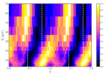
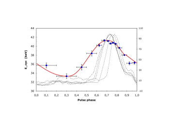
Throughout a full rotation of the neutron star we see the accretion mound or column under different angles. We therefore expect to observe significant changes in flux, in the shape of the continuum and in the CRSF parameters as function of pulse phase. The variation of flux as function of pulse phase is called the pulse profile. Each accreting pulsar has its own characteristic pulse profile which is often highly energy dependent. With increasing energy the pulse profiles tend to become smoother (less structured) and the pulsed fraction (the fraction of photons contributing to the modulated part of the flux) increases (Nagase, 1989; Bildsten et al., 1997). Furthermore, those profiles can vary from observation to observation, due to changes in the physical conditions of the accretion process, for example varying accretion rates. One way of presenting energy dependent pulse profiles is a two-dimensional plot: energy bins versus phase bins, with the flux coded by colors (see Fig. 3). In this plot horizontal lines represent pulse profiles (for selected energies) and columns represent spectra (for selected pulse phases). The centroid energy of cyclotron lines are generally also pulse phase dependent. The range of variability is from a few percent to 40% (see Table 6). As an example, Fig. 4 shows the variation of Ecyc for Her X-1 which is on the order of 25% (see Fig. 2 of Staubert et al. 2014).
In a simple picture, the changes of the CRSF energy are a result of sampling different heights of the line forming region as a function of pulse phase. Modeling these variations can help to constrain the geometry (under the assumption of a dipole magnetic field) of the accretion column with respect to the rotational axis as well as the inclination under which the system is viewed (see, e.g., Suchy et al., 2012). However, for a more physical constraint on those variations, the general relativistic effects such as light-bending around the neutron star have to be taken into account. These effects result in a large number of degrees of freedom, making it difficult to find a unique solution of the accretion geometry (Falkner et al., 2018).
In most sources, the strength of the CRSF depends strongly on pulse phase. In particular, the fundamental line is sometimes only seen at certain pulse phases, for example, Vela X-1 (Kreykenbohm et al., 2002) or KS 1947+300 (Fürst et al., 2014a). This behavior could indicate that the contributions of the two accretion columns vary and/or that the emission pattern during large parts of the pulse is such that the CRSF is very shallow or filled by spawned photons (Schwarm et al., 2017b). The latter model agrees with the fact that the harmonic line typically shows less depth variability with phase.
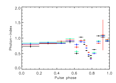
Continuum parameters are also known to change as function of pulse phase, but not necessarily in step with the observed CRSF variation (see Fig. 5). These changes can occur on all timescales, often varying smoothly as function of pulse phase (e.g., Suchy et al., 2008; Maitra & Paul, 2013b; Jaisawal & Naik, 2016, for a summary see Table 6). However, also sharp features are sometimes observed, where the spectrum is changing dramatically over only a few percent of the rotational period of the NS. The most extreme example is probably EXO 2030+375, where the photon-index changes by and the absorption column also varies by over an order of magnitude (Ferrigno et al., 2016b; Fürst et al., 2017). This effect is interpreted as an accretion curtain moving through our line of sight, indicating a unique accretion geometry in EXO 2030+375.
Another peculiar effect has been observed in the pulse profiles of some X-ray pulsars: the pulse profile shifts in
phase at the energy of the CRSFs (e.g., in 4U 0115+63; Ferrigno et al., 2011). This can be explained by the
different cross sections at the CRSF energies, leading to changes in emission pattern, as calculated by
Schönherr et al. (2014).

4.2 Cyclotron line parameters as function of luminosity
The spectral properties of several cyclotron line sources show a dependence on X-ray luminosity (). In particular, the cyclotron line energy was found to vary with in a systematic way, in correlation with the spectral hardness of the underlying continuum. Also the line width and depth of the cyclotron line(s) can vary. The first detection of a negative dependence of on Lx was claimed by Makishima et al. (1990a) and Mihara (1995) in high luminosity outbursts of three transient sources: 4U 0115+63, V 0332+53 and Cep X-4, observed by Ginga. “Negative” dependence means that decreases with increasing Lx. Fig. 6 shows the clear and strong negative correlation in V 0332+53 from observations by INTEGRAL and RXTE (Fig. 4 of Tsygankov et al. 2006). However, of the three sources’ dependencies originally quoted, only one, V 0332+53, can today be considered a secure result (Staubert et al., 2016): in Cep X-4 the effect was not confirmed (the source is instead now considered to belong to the group of objects with a “positive” dependence Vybornov et al. 2017). In 4U 0115+63, the reported negative (or anticorrelated) dependencies (Tsygankov et al., 2006; Nakajima et al., 2006; Tsygankov et al., 2007; Klochkov et al., 2011), have been shown to be most likely an artifact introduced by the way the continuum was modeled (Müller et al. 2013b, see also Iyer et al. 2015). More recently, a second source with a negative Ecyc/Lx correlation was found: SMC X-2 (see fig 9).
A simple idea about the physical reason for a negative correlation was advanced by Burnard et al. (1991). Based on Basko & Sunyaev (1976), who had shown that the height of the radiative shock above the neutron star surface (and with it the line forming region) should grow linearly with increasing accretion rate. They noted that this means a reduction in field strength and therefore a reduction of . Thus, with changing mass accretion rate, the strength of the (assumed dipole) magnetic field and should vary according to the law
| (8) |
where corresponds to the line emitted from the neutron star surface magnetic field , is the radius of the NS, and is the actual height of the line forming region above the NS surface. Regarding the physics of the scaling of the height of the line forming region see Sect. 5.1.
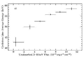
The first positive correlation (Ecyc increases with increasing Lx) was finally discovered in 2007 by Staubert et al. (2007) in Her X-1, a persistent medium luminosity source (Fig. 7). Since then six (possibly seven) more sources (all at moderate to low luminosities) have been found with Ecyc increasing with increasing luminosity (see Table 6): Vela X-1 (Fürst et al., 2014b; La Parola et al., 2016), A 0535+26 (Klochkov et al., 2011; Sartore et al., 2015), GX 304-1 (Yamamoto et al., 2011; Malacaria et al., 2015; Rothschild et al., 2017), Cep X-4 (Vybornov et al., 2017), 4U 1626.6-5156 (DeCesar et al., 2013), and V 0332+53 (the only source with a strong negative Ecyc / Lx correlation at high luminosities, see above) has been confirmed to switch to a positive correlation at very low flux levels at the end of an outburst (Doroshenko et al., 2017; Vybornov et al., 2018). A possible positive correlation in 4U 1907+09 (Hemphill et al., 2013) needs to be confirmed.
An interesting deviation from a purely linear correlation (only detectable when the dynamical range in Lx is sufficiently large) has recently been noticed in GX 304-1 and Cep X-4, namely a flattening toward higher luminosity (Rothschild et al., 2017; Vybornov et al., 2017) (see e.g., Fig. 8). This behavior is theoretically well explained by the model of a collisionless shock (see Sect. 5).
There are indications that in some objects the line width (and possibly the depth) also correlate with the luminosity (see Table 7) positively (at least up to a few times erg/s). This is not surprising since the line energy itself correlates with luminosity and the line width and depth generally correlate with the line energy (see Sect. 4.5). Measured values for the width and the depth of cyclotron lines are compiled in Table 7. However, the information on line width and depth are overall incomplete and rather scattered.
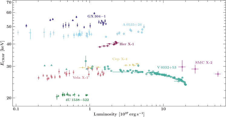
In the discovery paper of the positive Ecyc/Lx correlation in Her X-1, Staubert et al. (2007) had proposed, that for low to medium luminosity sources the physics of deceleration of the accreted matter close to the surface of the NS is very different from the case of the (transient) high luminosity sources: there is no radiation dominated shock that breaks the in-falling material (moving to larger heights when the accretion rate increases). Rather, the deceleration of the material is achieved through Coulomb interactions that produce the opposite behavior: for increasing accretion rate, the line forming region is pushed further down toward the NS surface (that is to regions with a stronger B-field), leading to an increase in Ecyc. This picture is supported by the theoretical work by Becker et al. (2012), that demonstrated that there are two regimes of high and low/medium accretion rates (luminosities), separated by a “critical luminosity” Lcrit on the order of erg/s. Fig. 9 is an updated version of Fig. 2 in Becker et al. (2012), showing our current knowledge of those sources that appear to show Ecyc/Lx correlations. For further details of the physics, which is clearly more complicated than the simple picture above, see Sect. 5 and the remarks about individual sources in Sect. 4.6.
For completeness, we mention alternative ideas regarding the luminosity dependence of Ecyc: for example, Poutanen et al. (2013), who – for high luminosity sources – follow the idea of an increasing height of the radiation dominated shock, but produce the CRSFs in the radiation reflected from larger and variable areas of the NS surface. We note, however, that it still needs to be shown that cyclotron absorption features can indeed be produced by reflection, and the model does not work for the positive correlation, which is – by far – the more frequently observed correlation. Mushtukov et al. (2015b), on the other hand, suggest that the varying cyclotron line energy is produced by Doppler-shift due to the radiating plasma, the movement of which depends on the accretion rate. A further extensive effort to model the luminosity dependence of Ecyc on luminosity by analytical calculations is from Nishimura (2008, 2011, 2013, 2014). By combining changes of the height and the area of the accretion mound with changes in the emission profile, he claims to be able to explain both – negative and the positive – Ecyc/Lx correlations.
4.3 Ecyc/Lx correlations on different timescales and line-continuum correlation
The original discoveries of the Ecyc/Lx correlations were based on observations with variation
of Lx on long timescales: days to months for the negative correlation (e.g., outburst of V 0332+53,
Tsygankov et al. 2006) and months to years for the first positive correlation in Her X-1 (Staubert et al., 2007).
It was first shown by Klochkov et al. (2011) that the same correlations are also observed on short timescales, that is on
timescales of individual pulses: a new technique of analysis was introduced the so-called pulse-to-pulse
or pulse-amplitude-resolved analysis. Most accreting pulsars exhibit strong variations in pulse flux (or amplitude),
due to variations in the accretion rate (or luminosity) on timescales at or below the duration of single pulses.
Any variations of the rate of capture of material at the magnetospheric boundary to the accretion disk are instantaneously
mirrored in the release of gravitational energy close to the surface of the neutron star (the free fall timescale is
on the order of milliseconds). So, in selecting pulses of similar amplitude and generating spectra of all photons in
those different groups, one can study the luminosity dependence of spectral parameters. Klochkov et al. (2011) analyse
observational data from INTEGRAL and RXTE of the two high-luminosity transient sources V 0332+53
and 4U 0115+63 as well as the medium to low luminosity sources Her X-1 and A 0535+26. The significance of this
work is twofold. First, the luminosity dependence of the cyclotron line energy as known from the earlier work (dealing with
long-term variations) is reproduced: the correlation is negative for the high luminosity sources and positive for the
medium to low luminosity sources. Second, the spectral index of the power law continuum varies with luminosity in the
same way as the cyclotron line energy: – correlates negatively (the spectra become softer) for the high
luminosity sources and positively (the spectra become harder, – get less negative) for the medium to low
luminosity sources.111111In contrast to earlier wording (e.g., Klochkov et al. 2011), we prefer to say:
Ecyc and – vary in the “same way”.
A supporting result with respect to the continuum was found by Postnov et al. (2015) who used
hardness ratios F(5-12 keV)/F(1.3-3 keV): in all sources analyzed the continuum becomes harder for increasing
luminosity up to Lx of (5-6) erg/s. For three objects where data beyond this luminosity were
available (EXO 2030+375, 4U 0115+63, and V 0332+53), the correlation changed sign (here we may see the
transition from subcritical to supercritical accretion – see Sect. 5.1).
In Table 6 we collate information about variations of Ecyc with pulse phase and with luminosity Lx and about changes of (or spectral hardness) with Lx. Those sources that show a systematic Ecyc/Lx correlation are discussed individually below. It is interesting to note that the sources with a positive correlation greatly outnumber those with the (first detected) negative correlation. We suggest that the positive correlation is a common property of low to medium luminosity accreting binary pulsars. It is also worth noting that the luminosity dependence of Ecyc is found on different timescales, ranging from years over days to seconds (the typical time frame of one pulse). Further details about the width and the depth of the cyclotron lines are compiled in Table 7. These parameters are also variable, but the information on this is, unfortunately, still rather scattered.
4.4 Long-term variations of the cyclotron line energy
So far, only two sources show a clear variability of the CRSF centroid energy over long timescales (tens of years): Her X-1 and Vela X-1. We discuss both sources below. For completeness, we mention 4U 1538-522 as a possible candidate for a long-term increase (Hemphill et al., 2016). Only further monitoring of this source over several years will tell whether the suspicion is justified. A peculiar variation on medium timescales (100 d) was observed in V 0332+53 during an outburst (Cusumano et al., 2016; Doroshenko et al., 2017; Vybornov et al., 2018) and from one outburst to the next (400 d) (Vybornov et al., 2018). During the outburst of June-September 2015 the source showed the well known anticorrelation of Ecyc with luminosity during the rise and the decay of the burst, but at the end of the burst the CRSF energy did not come back to its initial value (as was observed several times before). The data are consistent with a linear decay of Ecyc over the 100 d outburst by 5% (Cusumano et al., 2016). But at the next outburst, 400 d later, Ecyc had in fact resumed its original value of 30 keV. The physics of this phenomenon is unclear.
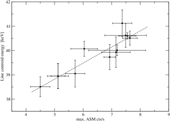
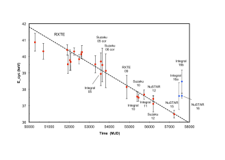
The first and best documented case for a long-term variation of the CRSF energy is Her X-1 (Staubert et al., 2007, 2014, 2016). At the time of discovery in 1976 the cyclotron line energy was around 37 keV (interpreted as absorption line). During the following 14 years several instruments (including the enlarged Balloon-HEXE, HEAO-A4, Mir-HEXE and Ginga) measured values between 33–37 keV (with uncertainties which allowed this energy to be considered well established and constant) (Gruber et al., 2001; Staubert et al., 2014). After a few years of no coverage, a surprisingly high value (44 keV) from observations with the GRO/BATSE instrument in 1993–1995 was announced (Freeman et al., 1996). Greeted with strong doubts at the time, values around 41 keV were subsequently measured by RXTE (Gruber et al., 1999) and BeppoSAX (Dal Fiume et al., 1998), confirming that the cyclotron line energy had indeed increased substantially between 1990 to 1993. Further observations then yielded hints for a possible slow decay. While trying to consolidate the evidence for such a decay, using a uniform set of RXTE observations, Staubert et al. (2007) instead found a new effect: a positive correlation between the pulse phase averaged Ecyc and the X-ray flux (or luminosity) of the source (Sect. 4.2), letting the apparent decrease largely appear as an artifact. However, with the inclusion of further data and a refined method of analysis, namely fitting Ecyc values with two variables (flux and time) simultaneously, it was possible to establish statistically significant evidence of a true long-term decay of the phase averaged cyclotron line energy by 5 keV over 20 years (Staubert et al., 2014; Staubert, 2014; Staubert et al., 2016). Both dependencies – on flux and on time – seem to be always present. The decay of Ecyc was independently confirmed by the analysis of Swift/BAT data (Klochkov et al., 2015). Further measurements, however, yield evidence that the decay of Ecyc may have stopped with a hint to an inversion (Staubert et al., 2017) (see Fig. 10). Since then, an intensified effort has been underway to monitor the cyclotron line energy with all instruments currently available. The analysis of the very latest observations between August 2017 and September 2018 seems to confirm this trend.
The physics of the long-term variation of Ecyc is not understood. We do, however, believe that this is not a sign of a change in the global (dipole) field of the NS, but rather a phenomenon associated with the field configuration localized to the region where the CRSF is produced. Apparently, the magnetic field strength at the place of the resonant scattering of photons trying to escape from the accretion mound surface must have changed with time. A few thoughts about how such changes could occur are advanced by Staubert et al. (2014, 2016) and Staubert (2014). Putting internal NS physics aside, changes could be connected to either a geometric displacement of the cyclotron resonant scattering region in the dipole field or to a true physical change in the magnetic field configuration at the polar cap. The latter could be introduced by continued accretion with a slight imbalance between the rate of accretion and the rate of “losing” material at the bottom of the accretion mound (either by incorporation into the neutron star crust or leaking of material to larger areas of the NS surface), leading to a change of the mass loading and consequently of the structure of the accretion mound: height or B-field configuration (e.g., “ballooning”, Mukherjee et al., 2013, 2014). It is also interesting to note that the measured Ecyc corresponds to a magnetic field strength ( Gauss) which is a factor of two larger than the polar surface field strength estimated from applying accretion torque models (see Sect. 6). This discrepancy could mean, that the B-field measured by Ecyc is for a local quadrupole field that is stronger and might be vulnerable to changes on short timescales (but see Sect. 6). Around 2015 the cyclotron line energy in Her X-1 seems to have reached a bottom value, comparable to the value of its original discovery (37 keV), with a possible slight increase (Staubert et al., 2017), leading to the question of whether we could – at some time – expect another jump upwards (as seen between 1990 and 1993).
Besides Her X-1, we know one more source with a long-term (over 11 yr) decay of the CRSF energy: Vela X-1 (La Parola et al., 2016). Vela X-1 is also one of seven sources showing a positive Ecyc/Lx dependence, originally discovered by Fürst et al. (2014b) and confirmed by La Parola et al. (2016). The same physics is probably at work in both sources. Most likely, more sources with this phenomenon will be found as monitoring, for example, with Swift/BAT, continues.
4.5 Correlations between Ecyc and other spectral parameters
Before entering discussion about the physics associated with the generation of X-ray spectra in general and cyclotron lines in particular, we briefly mention an interesting observational phenomenon: there are several correlations between spectral parameters of the continuum and those of the CRSFs. Historically, the first such correlation is that between the cutoff energy Ecutoff (see Eqs. (3) and (4)) and the CRSF centroid energy Ecyc, first noted by Makishima & Mihara (1992) (also Makishima et al. (1999), who realized that the relationship is probably not linear, but closer to Ecutoff E. Then a clear (linear) relationship was found between the width of the CRSF and the centroid energy Ecyc (Heindl et al., 2000; dal Fiume et al., 2000). It followed a systematic study in 2002 of all accreting pulsars showing CRSFs that were observed by RXTE (Coburn et al., 2002). Here, the above mentioned correlations were confirmed and one additional identified: the relative line width /Ecyc versus the optical depth of the line. As a consequence, almost every spectral parameter is – to some degree – correlated with all the others (see the correlation matrices, Tables 8 and 9 in Coburn et al., 2002). Through Monte Carlo simulations, Coburn et al. (2002) have shown that the correlations between the parameters are not an artifact (e.g., due to a mathematical coupling in the fitting process), but are actually of physical nature. Even though some ideas about the physical meaning of the observed correlations had been put forward, a rigorous check of the viability of those ideas is still needed.
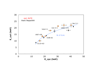
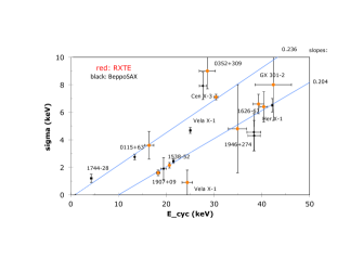
Recently, a similar systematic study using observational data from Beppo/SAX (on nearly the same set of objects, observed around the same time as by RXTE), was completed (PhD thesis Univ. of Tübingen by Doroshenko 2017).121212http://astro.uni-tuebingen.de/diss.shtml This study largely confirms the earlier results. Combining the results of both studies, two interesting features appear. First, the dependence of Ecutoff on Ecyc is even weaker, more like Ecutoff E (see Fig. 11). And second, the linear correlation Ecyc is well demonstrated (the data points from Beppo/SAX and RXTE are in good agreement). However, there is considerable scatter when all eleven objects are to be fit by one relationship. The scatter can be drastically reduced by assuming that there are two groups, both following the same slope, but with a constant offset of 2 keV in to one another (Fig. 12). The objects in the group with the smaller values appear to be the more “regular” objects, that tend to obey most other correlations fairly well. The objects in the other group are more often “outliers” in other correlations and have other or extreme properties, such as very high luminosity (Cen X-3, 4U 0115+63), a different continuum (4U 0352+309), or are otherwise peculiar, as is the bursting pulsar (4U 1744-28). Generally we find that as the width and depth of the CRSF increase with increasing centroid energy Ecyc, two continuum parameters also increase: the cut-off energy Ecutoff and the power law index (the continuum hardens).
4.6 Individual sources
Here we summarize the main characteristics of all sources showing a correlation between Ecyc and Lx.
We start with sources of low to medium luminosity showing a positive correlation (seven sources),
followed by the two sources at very high luminosities showing a negative correlation.
Her X-1: This source is in many ways unique: it belongs to the class of low mass accreting binary pulsars with the highly magnetized neutron star accreting through an accretion disk. The optical companion, HZ Hercules, is a low mass main sequence star with spectral type A to F. It was known well before the discovery of the X-ray source as an interesting variable star. The optical light is modulated at the binary period of 1.70 d due to heating by the X-rays from the neutron star. A long-term optical history, showing periods of extended lows, is documented on several photographic plates from different observatories, dating back to 1890 (Jones et al., 1973). The binary system shows a large number of observational features (also due to the low inclination of its binary orbit), that are characteristic for the whole class of objects. Apart from being one (together with Cen X-3) of the two first detected binary X-ray pulsars (Tananbaum et al., 1972), Her X-1 is associated with several other “first detections” (see e.g., Staubert, 2014), in particular with respect to cyclotron line research: 1) the detection of the first cyclotron line ever (Fig. 1) (Trümper et al., 1977, 1978), constituting the first “direct” measurement of the magnetic field strength in a neutron star, 2) the detection of the first positive correlation of the cyclotron line energy Ecyc with X-ray luminosity (Staubert et al., 2007) (see Sect. 4.3), and 3) the first detection of a long-term decay of Ecyc (by keV over 20 yrs) (Staubert et al., 2014, 2016) (see Sect. 4.4).
The positive correlation is also found on a timescale of seconds using the “pulse-to-pulse” (or “amplitude-resolved”
analysis) (Klochkov et al., 2011) (see Sect. 4.3). In this analysis it is demonstrated that, together with
the cyclotron line energy, the continuum also varies: for Her X-1 the continuum gets harder (the power law index
decreases, increases) with increasing Lx. This appears to hold for all objects with a positive
Ecyc/Lx correlation and the opposite is true for that with a negative Ecyc/Lx correlation.
In addition, Her X-1 is one of the few binary X-ray pulsars exhibiting a super-orbital period of 35 days, strongly modulating
the overall X-ray flux as well as the shape of the pulse profile (see e.g., Staubert, 2014). This modulation is thought to be
due to an obscuration of the areas on the neutron star surface where X-rays are produced by the accretion disk. The super-orbital
modulation is not a good clock and has its own quite intriguing timing properties (Staubert et al., 2010c, 2013, 2014).
It is an open question whether the suggestion of free precession of the neutron star
(Trümper et al., 1986; Staubert et al., 2009, 2010a, 2010b; Postnov et al., 2013) is indeed viable.
It is interesting to note that Ecyc appears to change slightly with 35d-phase (Staubert et al., 2014).
GX 3041: Originally discovered at hard X-ray energies (above 20 keV) during a set of MIT balloon scans
of the Galactic plane in the late 1960s and early 1970s (McClintock et al., 1971), and seen as an UHURU
source at 210 keV (Giacconi et al., 1972), the source went into quiescence for nearly 30 years (Pietsch et al., 1986)
until its re-emergence in 2008 (Manousakis et al., 2008). The binary orbit is 132.2 d (from the separation between outbursts,
(Sugizaki et al., 2015; Yamamoto et al., 2011; Malacaria et al., 2015)), and the pulse period is 275 s (McClintock et al., 1977).
The star V850 Cen was identified as the optical companion (Mason et al., 1978). The first detection of a cyclotron line at 54 keV
and its possible luminosity dependence is based on RXTE observations of an outburst in August 2010 (Yamamoto et al., 2011).
The positive luminosity correlation was confirmed through INTEGRAL results (Klochkov et al., 2012; Malacaria et al., 2015).
Recent analysis of all of the RXTE observations of GX 3041 by Rothschild et al. (2016, 2017) covered four
outbursts in 2010 and 2011. This analysis not only confirmed the positive correlation of the CRSF energy with luminosity,
but also showed a positive correlation of the line width and depth with luminosity. In addition, a positive correlation was seen
for the power law index (the spectrum getting harder with increasing luminosity) and for the iron line flux. For the first time,
all the CRSF correlations were seen to flatten with increasing luminosity (see Fig.8).
As will be discussed in Sect. 5, this behavior can be successfully modeled assuming a slow down of the
accretion flow by a collisionless shock, in which the radiation pressure is of minor importance.
Vela X-1: An eclipsing high-mass X-ray binary discovered in the early years of X-ray astronomy by Chodil et al. (1967), this source is considered as an archetypal wind accretor. It is a persistent source with essentially random flux variations explained by accretion from a dense, structured wind surrounding the optical companion HD 77581(e.g., Fürst et al., 2014b). HD 77581 is a 24 main sequence giant in a binary orbit of 8.96 d and moderate eccentricity (e = 0.09).
The first evidence for cyclotron lines in this source – a fundamental around
25 keV and a first harmonic near 50 keV – was found by Kendziorra et al. (1992)
using Mir-HEXE and further detailed by Kretschmar et al. (1996).
Early observations with RXTE confirmed these detections
(Kretschmar et al., 1997). Based on NuSTAR observations,
Fürst et al. (2014b) reported a clear increase of the energy of the
harmonic line feature with luminosity, the first clear example for such
behavior in a persistent HMXB. In contrast, the central energy of the
fundamental line shows a complex evolution with luminosity, which might be
caused by limitations of the phenomenological models used.
From a study of long-term data of Swift/BAT, La Parola et al. (2016)
confirmed the positive correlation of the harmonic line energy with luminosity
and noted, that the fundamental line is not always present.
In addition, they found a secular variation of the line energy, decreasing by
0.36 keV yr-1 between 2004 and 2010. This establishes Vela X-1
as the second source (after Her X-1) for which a long-term decay is observed.
A 0535+26: The transient X-ray binary A 053526 was discovered in outburst during observations of the Crab with the Rotation Modulation Collimator on Ariel V, showing X-ray pulsations of 104 s (Rosenberg et al., 1975). The system was found to consist of an O9.7IIIe donor star and a magnetized neutron star (Liller, 1975; Steele et al., 1998). It has an eccentricity of and an orbital period of d (Finger et al., 1996). The distance to A 053526 is 2 kpc (Giangrande et al., 1980; Steele et al., 1998), which has been recently confirmed by Gaia (Bailer-Jones et al., 2018).
Absorption line-like features at 50 and 100 keV, where the former was of low significance, were first detected with MIR TTM/HEXE during a 1989 outburst of the source (Kendziorra et al., 1994). They were interpreted as the fundamental and first harmonic cyclotron resonances. An 110 keV feature was confirmed with CGRO OSSE during a 1994 outburst (Grove et al., 1995, with no definite statement on the presence of the low energy line due to OSSE’s 45 keV threshold). In the following years the fundamental line was independently confirmed near 46 keV with different missions during a 2005 August/September outburst (Kretschmar et al., 2005; Wilson et al., 2005; Inoue et al., 2005) and it has been studied for several outbursts since then (e.g., Ballhausen et al., 2017).
The outbursts of A 053526 show varying peak brightnesses, reaching
15–50 keV fluxes from a few 100 mCrab to 5.5 Crab
(Camero-Arranz et al., 2012a; Caballero et al., 2013a). Bright, so-called giant
outbursts are known to have occured in 1975, 1980, 1983, 1989, 1994,
2005, 2009, and 2011 (Caballero et al., 2007, 2013b, 2013a, and references
therein). The source has
been observed over a large range of luminosities. High quality data
could be obtained down to comparatively low outburst luminosities
(Terada et al., 2006; Ballhausen et al., 2017) and even in quiescence
(Rothschild et al., 2013). The fundamental cyclotron line energy generally
does not change significantly with luminosity (over a wide range) (see
Fig. 9 and, e.g., Caballero et al., 2007). There are,
however, tantalizing indications for a more complex behavior: (i)
clear increase of the line energy up to keV was
observed for a flare during the rising phase of the 2005 giant
outburst (Caballero et al., 2008), (ii) similar to Her X-1 a positive
/ correlation was found using the
“pulse-to-pulse” analysis (Klochkov et al., 2011; Müller et al., 2013a), and (iii)
the positive correlation might also be visible at the highest
luminosities (see Fig. 9 and, e.g., Sartore et al., 2015).
The continuum emission of A 053526 has been observed to harden
with increasing luminosity (Klochkov et al., 2011; Caballero et al., 2013b), with
possible saturation at the highest luminosities (Postnov et al., 2015) and
a more strongly peaked rollover at the lowest outburst luminosities
(Ballhausen et al., 2017).
Cep X-4: This source was discovered by OSO-7 in 1972 (Ulmer et al., 1973). During an outburst in
1988 observed by Ginga, regular pulsations with a pulse period around 66 s were discovered,
and evidence for a CRSF around 30 keV was found (Mihara et al., 1991). The optical counterpart was
identified by Bonnet-Bidaud & Mouchet (1998), who measured a distance of kpc.
Mihara (1995), on the basis of Ginga observations, had claimed that Cep X-4 (together with the high
luminosity sources 4U 0115+63 and V 0332+53) showed a negative Ecyc/Lx correlation.
This has never been confirmed. Instead a positive correlation was discovered in NuSTAR data
(Fürst et al., 2015) – although with two data points only. Jaisawal & Naik (2015b) detected the first harmonic
in observations by Suzaku. Vybornov et al. (2017), analyzing an outburst observed in 2014 by
NuSTAR using the pulse-amplitude-resolving technique (Klochkov et al., 2011) confirmed the existence
of the two cyclotron lines at 30 keV and 55 keV and found a strong positive Ecyc /
Lx correlation, that is well modeled by assuming a collisionless shock.
Swift 1626.65156: The source was discovered by Swift/BAT during an outburst in
2005 as a transient pulsar with 15 s pulse period (Palmer et al., 2005). The optical companion was identified
as a Be-star (Negueruela & Marco, 2006). After different suggestions, a convincing orbital solution was finally found
by Baykal et al. (2010) with a period of 132.9 d and a very small eccentricity (0.08).
Several observations over three years (2006–2008) by RXTE/PCA led to the discovery of a CRSF at
about 10 keV (DeCesar et al., 2013). Even though the discovery of this CRSF needs confirmation by
further observations (and other instruments), we list this source not under the category “candidates” because the
evidence from the different observations is quite strong and there are clear signatures of the usual behavior
of CRSFs, including a strong correlation of the phase resolved CRSF energy with pulse phase, an indication for a positive
correlation with luminosity and a hint to a first harmonic at 18 keV.
V 0332+53: The transient X-ray binary V 033253 was discovered in outburst in 1983 by Tenma (Tanaka, 1983; Makishima et al., 1990b) and in parallel an earlier outburst was revealed in Vela 5B data from 1973 (Terrell & Priedhorsky, 1983, 1984). In follow-up observations by EXOSAT during the 1983 activity, 4.4 s pulsations were discovered, an accurate position was measured, and the orbital period and eccentricity were determined to be 34 days and 0.37, respectively (Stella et al., 1985, see also Zhang et al. 2005). The O8–9Ve star BQ Cam was identified as the optical counterpart (Argyle et al., 1983; Negueruela et al., 1999). The distance to the system was estimated to be 6–9 kpc (Negueruela et al., 1999, but see also Corbet et al. 1986).
V 033253 displays normal as well as giant outbursts. Occurrences of the latter have been observed in 1973, 2004/2005, and 2015 (Ferrigno et al., 2016a). During giant outbursts the source can become one of the most luminous X-ray sources in the Galaxy, reaching a few times . Quasi-periodic oscillations with frequencies of 0.05 Hz and 0.22 Hz have been observed (Takeshima et al., 1994; Qu et al., 2005; Caballero-García et al., 2016).
The Tenma observation of V 033253 also provided evidence for a fundamental cyclotron line feature at 28 keV (Makishima et al., 1990b). Its presence was confirmed with high significance by Ginga observations of the source during a 1989 outburst, which also showed indications for a harmonic feature at 53 keV (Makishima et al., 1990a). The giant outburst in 2004/2005 allowed for the confirmation of this harmonic as well as the detection of a rare second harmonic at 74 keV with INTEGRAL and RXTE (Kreykenbohm et al., 2005; Pottschmidt et al., 2005).
These observations of the giant outburst in 2004/2005 further revealed that the energy of the fundamental cyclotron line decreased with increasing luminosity (Tsygankov et al., 2006, 2010; Mowlavi et al., 2006). Additional studies showed that the correlation was also present for the first harmonic line (although characterized by a weaker fractional change in energy, Nakajima et al., 2010) as well as for the pulse-to-pulse analysis of the fundamental line (Klochkov et al., 2011). A qualitative discussion of results from pulse phase-resolved spectroscopy of this outburst in terms of the reflection model for cyclotron line formation has been presented (Poutanen et al., 2013; Lutovinov et al., 2015). Swift, INTEGRAL, and NuSTAR observations of the most recent giant outburst in 2015 also showed the negative correlation and provided evidence that the overall line energy, and thus the associated -field, was lower just after the outburst, indicating some decay over the time of the outburst (Cusumano et al., 2016; Ferrigno et al., 2016a; Doroshenko et al., 2017; Vybornov et al., 2018) (see also the discussion in Sect. 4.4).
V 033253 is singled out by the fact that it is the only source to date in which we
find both Ecyc / Lx correlations: the negative at high luminosities and the
positive at low luminosity (Doroshenko et al., 2017; Vybornov et al., 2018).
It is also the only one with a very strong negative correlation,
accompanied by a second source – SMC X-2 – which shows a much weaker dependence
(see Fig. 9). This two-fold behavior is in line with the correlation between
the spectral index (or spectral hardening) as found in several other accreting pulsars:
a hardening at low luminosities and a softening at very high luminosities
(Klochkov et al., 2011; Postnov et al., 2015).
SMC X-2: This transient source in the Small Magellanic Cloud was detected
by SAS-3 during an outburst in 1977 (Clark et al., 1978, 1979). Later outbursts were observed by
several satellites. In 2000 the source was identified as an X-ray pulsar by RXTE and ASCA with a
period of 2.37 s (Torii et al., 2000; Corbet et al., 2001; Yokogawa et al., 2001). The optical companion suggested by
Crampton et al. (1978) was later resolved into two objects and the northern one identified as the true companion
based on an optical periodicity of 18.6 d (Schurch et al., 2011), that appeared to coincide with an
X-ray period of 18.4 d found in RXTE data (Townsend et al., 2011). The optical classification
of the companion was determined to be O9.5 III-V (McBride et al., 2008). During an outburst in 2015
Jaisawal & Naik (2016) found a cyclotron line at 27 keV in NuSTAR data, that showed a weak
negative correlation with luminosity (see Fig. 9). If this is confirmed, SMX X-2 is the second
high luminosity source showing this negative correlation with luminosity. As with Swift 1626.6-5156, the detection
of the cyclotron line needs confirmation. Lutovinov et al. (2017a), using observations by Swift/XRT of the same
outburst in 2015, detected a sudden drop in luminosity to below a few times erg/s, which,
interpreted as the signature of the propeller effect, allows us to estimate the strength of the magnetic field to be around
3 Gauss. This is quite close to the B-field value found from the cyclotron line energy
(see also Sect. 6).
4U 0115+63: This source is included here since, historically, it was thought to be a high luminosity source showing a negative Ecyc / correlation. As we discuss below, we now believe, however, that this is probably not correct. 4U 0115+63 is a high mass X-ray binary system, first discovered in the sky survey by UHURU (Giacconi et al., 1972), with repeated outbursts reaching high luminosities (Boldin et al., 2013). The system consists of a pulsating neutron star with a spin period of 3.61 s (Cominsky et al., 1978) and a B0.2Ve main sequence star (Johns et al., 1978), orbiting each other in 24.3 d (Rappaport et al., 1978). The distance to this system has been estimated at 7 kpc (Negueruela & Okazaki, 2001). As early as 1980 a cyclotron line at 20 keV was discovered in 4U 0115+63 in observational data of HEAO-1/A4 (Wheaton et al., 1979). A re-examination of the data uncovered the existence of two lines at 11.5 and 23 keV which were immediately interpreted as the fundamental and harmonic electron cyclotron resonances (White et al., 1983). Later observations of the source found three (Heindl et al., 1999), then four (Santangelo et al., 1999), and finally up to five lines in total (Heindl et al., 2004). 4U 0115+63 is still the record holder in the numbers of harmonics.
A negative correlation between the pulse phase averaged cyclotron line energy and the X-ray luminosity (a decrease in Ecyc with increasing ) was claimed for the first time in this source by Mihara (1995) on the basis of observations with Ginga (together with two other high luminosity transient sources: Cep X-4, and V 0332+53). This negative correlation was associated with the high accretion rate during the X-ray outbursts, and as due to a change in height of the shock (and emission) region above the surface of the neutron star with changing mass accretion rate, . In the model of Burnard et al. (1991), the height of the polar accretion structure is tied to (see above). A similar behavior was observed in further outbursts of 4U 0115+63 in March-April 1999 and Sep-Oct 2004: both Nakajima et al. (2006) and Tsygankov et al. (2007) had found a general anticorrelation between Ecyc and luminosity. The negative correlation was also confirmed by Klochkov et al. (2011) using the pulse-amplitude-resolved analysis technique, together with the softening of the continuum when reaching very high luminosities (see also Postnov et al. 2015).
However, Müller et al. (2013b), analyzing data of a different outburst of this source in March-April 2008, observed by RXTE and INTEGRAL, have found that the negative correlation for the fundamental cyclotron line is likely an artifact due to correlations between continuum and line parameters when using the NPEX continuum model. Further, no anticorrelation is seen in any of the harmonics. Iyer et al. (2015) have suggested an alternative explanation: there may be two systems of cyclotron lines with fundamentals at 11 keV and 15 keV, produced in two different emission regions (possibly at different poles). In this model, the second harmonic of the first system coincides roughly with the 1st harmonic in the second system. In summary, we conclude that 4U 0115+63 does not show an established dependence of a CRSF energy on luminosity.
5 Physics of the accretion column
In this Section we discuss the basic physics with relevance to the accretion onto highly magnetized neutron stars. The generation of the X-ray continuum and the cyclotron lines, as well as their short- and long-term variability, depends on the structure of the accretion column, the physical state of the hot magnetized plasma, the magnetic field configuration and many details with regard to fundamental interaction processes between particles and photons that govern the energy and radiation transport within the accretion column.
Our basic understanding is that material transferred from a binary companion couples to the magnetosphere of the neutron star (assuming a simple dipole field initially). The accreted plasma falls along the magnetic field lines down to the surface of the NS onto a small area at the polar caps, where it is stopped and its kinetic energy is converted to heat and radiation. From the resulting “accretion mound” the radiation escapes in directions that depend on the structure of the mound, the B-field and the gravitational bending by the NS mass. If the magnetic and spin axes of the neutron star are not aligned, a terrestrial observer sees a flux modulated at the rotation frequency of the star.
We refer to the following fundamental contributions to the vast literature on this topic: Gnedin & Sunyaev (1974); Lodenquai et al. (1974); Basko & Sunyaev (1975); Shapiro & Salpeter (1975); Wang & Frank (1981); Langer & Rappaport (1982); Braun & Yahel (1984); Arons et al. (1987); Miller et al. (1987); Meszaros (1992); Nelson et al. (1993); Becker et al. (2012). Further references are given in the detailed discussion below.
5.1 Accretion regimes
In the simplest case of a dipole magnetic field, the plasma filled polar cap area is with polar cap radius , where is the magnetospheric radius. The latter is determined by the balance of the magnetic field and matter pressure, and is a function of the mass accretion rate and the NS magnetic field, which can be characterized by the surface NS value, , or, equivalently, by the dipole magnetic moment - see footnote.131313We note that the factor of a half, required by electrodynamics describing the B-field at the magnetic poles (see e.g., Landau-Lifschits, Theory of fields), is often missing in the literature (see also the comments in Table 1). The accreting matter moves toward the NS with free-fall velocity, which is about cm s-1 close to the NS. The matter stops at (or near) the NS surface, with its kinetic energy being ultimately released in the form of radiation with a total luminosity of . The continuum is believed to be due to thermal bremsstrahlung radiation from the 108 K hot plasma, blackbody radiation from the NS surface and cyclotron continuum radiation - all modified by Comptonisation (Basko & Sunyaev, 1975; Becker & Wolff, 2007; Becker et al., 2012) and the cyclotron line by resonant scattering of photons on electrons with discrete energies of Landau levels (Ventura et al., 1979; Bonazzola et al., 1979; Langer et al., 1980; Nagel, 1980; Meszaros et al., 1983).
Since the discovery of negative and positive / correlations, first found for V 0332+53 (Makishima et al., 1990a; Mihara, 1995) and Her X-1 (Staubert et al., 2007), respectively, it has become very clear that there are different accretion regimes, depending on the mass accretion rate (X-ray luminosity). An important value separating low and high accretion rates is the “critical luminosity”, erg s-1 (see below). The different accretion regimes correspond to different breaking regimes, that is, different physics by which the in-falling material is decelerated. So, the study of the / dependence provides a new tool for probing physical processes involved in stopping the accretion flow above the surface of strongly magnetized neutron stars in accreting X-ray pulsars.
The different breaking regimes are as follows. If the accretion rate is very small, the plasma blobs frozen in the NS magnetosphere arrive almost at the NS surface without breaking, and the final breaking occurs in the NS atmosphere via Coulomb interactions, various collective plasma processes and nuclear interactions. This regime was first considered in the case of spherical accretion onto NS without magnetic fields by Zel’dovich & Shakura (1969) and later in the case of magnetized neutron stars (e.g., Miller et al. 1987; Nelson et al. 1993). The self-consistent calculations of the layer in which energy of the accreting flow was released carried out in these papers showed that the stopping length of a proton due to Coulomb interactions amounts to 50 g cm-2, where is the plasma density and the height of this layer is comparable to the NS atmosphere size. Clearly, in this case the CRSF feature (if measured) should reflect the magnetic field strength close to the NS surface and should not appreciably vary with changing accretion luminosity
With increasing mass accretion rate , the accreting flow (treated gas-dynamically) starts decelerating with the formation of a collisionless shock (CS). The possibility of deceleration via a CS was first considered in the case of accretion of plasma onto a neutron star with a magnetic field by Bisnovatyi-Kogan & Fridman (1970). Later several authors (e.g., Shapiro & Salpeter 1975; Langer & Rappaport 1982; Braun & Yahel 1984) postulated the existence of a stationary CS above the neutron star surface if the accretion luminosity is much less than the Eddington luminosity. The formation and structure of the CS, in this case, accounting for detailed microphysics (cyclotron electron and proton cooling, bremsstrahlung losses, resonant interaction of photons in diffusion approximation, etc.), is calculated numerically by Bykov & Krasil’shchikov (2004) in 1D-approximation. These calculations confirmed the basic feature of CS: (1) the formation above the neutron star surface at the height , where is the upstream velocity, and is the equilibration time between protons and electrons via Coulomb interactions, which follows from the requirement to transfer most of the kinetic energy carried by ions to radiating electrons, (2) the release of a substantial fraction (about half) of the in-falling kinetic energy of the accretion flow downstream of the CS in a thin interaction region of the flow.
The CS breaking regime persists until the role of the emitted photons becomes decisive, which can be quantified (to an order of magnitude) by equating the photon diffusion time across the accretion column, , where is the photon mean free path in the strong magnetic field, and the free-fall time of plasma from the shock height, . This relation yields the so-called “critical luminosity”, erg s-1, above which the in-falling accretion flow is decelerated by a radiative shock (RS) (Basko & Sunyaev, 1975, 1976; Arons et al., 1987). In the literature, there are several attempts to calculate this critical luminosity (which should depend on the magnetic field, the geometry of the flow, etc.) more precisely (see e.g., Wang & Frank, 1981; Becker et al., 2012; Mushtukov et al., 2015a). It should be kept in mind, however, that the transition to a radiation dominated (RD)-dominated regime occurs rather smoothly, and this critical luminosity should be perceived as a guidance value (and not a strict boundary) for the separation between the pure CS or RS regimes in a particular source.
5.1.1 Scaling CRSF relations in collisionless shock regime
In the CS regime that can be realized in accreting X-ray pulsars with low or moderate X-ray luminosity (e.g., Her X-1, GX 304-1, Cep X-4, etc.), there are simple and physically clear relations between the CRSF properties (energy, width, depth) and X-ray luminosity, which have been checked by X-ray observations. Indeed, the typical CS height is a few hundred meters above the neutron star surface and scales with the plasma number density as and, through the mass conservation , as (Shapiro & Salpeter, 1975; Basko & Sunyaev, 1976), confirmed through detailed numerical simulations by Bykov & Krasil’shchikov 2004 (see their Fig. 5). At these heights, the dipole structure of the neutron star magnetic field is already important. The theory of CRSF formation in an inhomogeneous magnetic field can be found in Zheleznyakov (1996). In the inhomogeneous magnetic field, the cyclotron line is formed in a resonant layer. The width of the resonant layer for the assumed dipole magnetic field is , where is the thermal velocity of post-shock electrons and is the radial height of the resonant layer; for typical temperatures keV and cyclotron photon energies 30-50 keV, the size of the resonant layer cm can be comparable with the shock height and thus can substantially affect the CRSF formation. We note that the post-shock electron temperature does not vary substantially.
The characteristic optical depth of the resonant layer in the inhomogeneous dipole magnetic field is (Zheleznyakov, 1996)
| (9) |
This means that diffusion of resonant photons occurs.
As the CS downstream sidewall area is typically smaller than the polar
cap area (at least if ), most of the diffusing photons escape
from the uppermost parts of the structure.
Clearly, the line dependence on the observed X-ray flux is entirely determined by how the collisionless shock height responds to variable mass accretion rate. This scaling indeed was first observed in Her X-1 and explained in terms of the line formation in the varying magnetic field with height in Staubert et al. (2007). As discussed above, we now know four additional X-ray pulsars presumably in the CS breaking regime, showing a positive / correlation: Vela X-1, A 0535+26, GX 304-1, Cep X-4 (see 4.2). A factor five to six in the dynamic range in has allowed for the last two objects to detect the theoretically expected deviations from a purely linear correlation. We note that not only the energy , but also its width and depth show variations with the observed X-ray flux, consistent with this non-linear scaling (see Rothschild et al. 2017 for more detail), thus lending credence to the simple physical picture outlined above.
5.1.2 Scaling CRSF relations in radiative shock regime
In the case of RS deceleration of the accretion flow at high X-ray luminosities, the situation with CRSF formation is not so straightforward as in the CS-regime considered above. Indeed, in this case an optically thick extended intrinsically 2D structure is formed (Davidson, 1973; Basko & Sunyaev, 1976; Wang & Frank, 1981; Postnov et al., 2015), and the line formation should be calculated by solving the 2D radiation transfer problem. Still, the assumption that the shock height (and the line emitting region) should increase with increasing mass accretion rate (Basko & Sunyaev, 1976) should hold, and should vary according to Eq. 8, as first suggested by Burnard et al. (1991). In addition, reflection of radiation from the neutron star surface could play a role. While physically feasible, the reflection model for CRSF formation and change with X-ray flux in high-luminosity accreting X-ray pulsars advanced by Poutanen et al. (2013) may not be universally applied in all cases, since the negative CRSF correlation with luminosity is now reliably confirmed by X-ray observations of only one bright transient X-ray pulsar V0332+53 (Tsygankov et al., 2006) and tentatively diagnosed for SMC X-2 (Jaisawal & Naik, 2016). Clearly, future observations (possibly, with X-ray polarization measurements) are needed here to study the intriguing CRSF behavior in the RS-case.
5.2 Cyclotron line modeling
This paper concentrates on the observational aspects of objects from which spectra with cyclotron lines are observed. A description of the state of theoretical modeling of the CRSF is beyond the scope of this contribution – a comprehensive review as a counterpart would, however, be highly useful.
In the Introduction and in Sect. 5 above mention the history of the early theoretical work that attempted to calculate expected spectra analytically and that has been ground breaking for our understanding of the basic physics in highly magnetized hot plasma – the source of high energy X-ray spectra with cyclotron lines. Wang et al. (1988) give a good summary of the early work, which is mostly from the 70s and 80s of the last century. More recent analytical calculations are from Nishimura (2008, 2011, 2013, 2014, 2015). Nishimura invokes several specific conditions, for example, changes of the height and the area of the accretion mound, changes in the emission profile, non-uniform illumination of the emission region, superposition of lines from different regions, changing relative contributions from the two accreting poles and other, to explain observational details. The success of this may, however, be due to a large number of free parameters and/or assumptions that enter the calculations from the start.
A completely different technique to understand and model the physical conditions that lead to the observed cyclotron line spectra are Monte Carlo calculations (Isenberg et al., 1998; Araya & Harding, 1999; Araya-Góchez & Harding, 2000; Schönherr et al., 2007; Nobili et al., 2008; Schwarm et al., 2017b, a). Here individual particles (electrons, photons, protons) are followed through some extended volume of highly magnetized hot plasma, calculating their interactions with each other and with the magnetic field. At the boundaries of the volume photons escape, some of them finding their way into the telescopes of observers, where the energy distribution (spectra) and the timing distribution (pulse profiles and other time variations) are measured. Usually, some input continuum spectrum is chosen that illuminates a certain volume under specific geometries. The method is rather flexible, allowing for the testing of different input continua and geometries (e.g., illumination from the bottom, from the top, from a centrally extended source, or others), and angle- and energy dependent interaction cross-sections can easily be adjusted. The most recent and complete calculations are by Fritz Schwarm141414Schwarm: PhD Thesis, University of Erlangen-Nürnberg, https://www.sternwarte.uni-erlangen.de/docs/theses/2017-05_Schwarm (Schwarm et al., 2017b, a). This work represents the current state of the art and provides, for the first time, a framework (usable by the general scientific community)151515https://www.sternwarte.uni-erlangen.de/ schwarm/public/cyclo for a direct comparison and fitting of observed spectra with Monte-Carlo-simulated spectra, such that physical conditions and parameters can be estimated.
| System | Refer.a | (GL)c | B12 =e | Cyclotron | B12 | B(Wang) | Btorque |
| “rotator” b | or | 2 | line | from | / B(GL) | / Bcyc | |
| (Wang) =d | = Btorque | Energy | Ecyc | or | |||
| 5(Wang) | Ecyc | (= Bcyc) | B(Klus) | ||||
| [] | [ G] | [keV] | [ G] | / B(GL) | |||
| Her X-1 | GL“fast” | 0.47g | 0.94 | 37 | 3.83 | 2.2 | 0.25 |
| ” ” ” | Wang | 1.05 | 2.10 | 37 | 3.83 | 0.55 | |
| GX 301-2 | GL “slow” | 0.3 | 0.6 | 37 | 3.83 | 0.16 | |
| 4U 0115+63 | GL “fast” | 1.4 | 2.8 | 12 | 1.24 | 2.1 | 2.3 |
| ” ” ” | Wang | 2.95 | 5.9 | 12 | 1.24 | 4.8 | |
| 4U 1626-67 | Wang | 4.35 | 8.7 | 37 | 3.83 | 2.3 | |
| A 0535+26 | GL “slow” | 3.3 | 6.6 | 50 | 5.17 | 2.1 | 1.3 |
| ” ” ” | Klus | 14 | 50 | 5.17 | 2.7 | ||
| Cen X-3 | GL “fast” | 4.5 | 9 | 28 | 2.90 | 2.1 | 3.1 |
| ” ” ” | Wang | 9.55 | 19.1 | 28 | 2.90 | 6.6 | |
| X Per | GL “slow” | 4.8 | 9.6 | 29 | 2.19 | 4.4 | |
| ” ” ” | GL “slow” | 4.8 | 9.6 | 29 | 2.19 | 4.4 | |
| ” ” ” | Klus | 42 | 29 | 2.19 | 19.2 | ||
| Vela X-1h | GL “fast” | 86 | 172 | 25 | 2.60 | 66 | |
| A 0535+26 | GL “fast” | 148 | 296 | 50 | 5.17 | 57 | |
| GX 301-2 | GL “fast” | 394 | 788 | 37 | 3.83 | 206 |
a References: “GL” : Ghosh & Lamb (1979b), “Wang” : Wang (1987), “Klus” : Klus et al. (2014);
b ”slow” or “fast” solution according to Ghosh & Lamb (1979b),
c original values from the literature;
d the original values of Wang (1987) are , = 5;
e we use the definition: B = 2 (unlike Ghosh & Lamb 1979a, see text) and consider this to be the field strength
B0 at the surface of the neutron star at the magnetic poles;
g we note that =0.47 is a valid solution for Her X-1 within the GL-model, but it requires L37=2.7
(not 1.0, as in Table 1 of Ghosh & Lamb 1979b);
h for Vela X-1 the GL “slow” solution yields = , obviously not valid.
6 Empirical knowledge of the magnetic field strength of a neutron star
Even though we assume that the observation of the cyclotron line energy gives a direct measure of the strength of the magnetic field at the site where the resonant scattering occurs, it does not provide an accurate value for the global magnetic field (thought to be a dipole). This is because the cyclotron scattering region may be at some distance above the neutron star surface, and/or there may be local field structures which could have a different (even stronger) field strength. A classical method to estimate the magnetic moment of a neutron star is to infer it through timing observations of pulsars. This has been done for non-accreting pulsars by applying the theory of dipole radiation to observational data of the change of the pulse period with time (Gold, 1968; Goldreich & Julian, 1969; Ostriker & Gunn, 1969): B = 3.2, with B in Gauss, P in s and in s s-1 (leading, e.g., to an estimate of the field strength of the Crab pulsar of Gauss). In the case of accreting pulsars – relevant for cyclotron line objects discussed here – accretion torque models are applied to describe the spin-up/spin-down behavior observed in these objects. The most widely used model, applicable to the accretion through an accretion disk, is the one developed by Ghosh & Lamb (1979b) (Paper III) (with the preceding Paper I: Ghosh et al. 1977 and Paper II: Ghosh & Lamb 1979a). The model provides a set of equations for the relationship between the magnetic moment of the neutron star and the three observables: pulse period P, its time derivative dP/dt and the X-ray luminosity Lx (estimated through the X-ray flux and the distance to the source), and two unknown quantities: the magnetic moment and a dimensionless torque parameter , which itself is a complicated function of a “fastness parameter” (the ratio of the magnetospheric radius to the co-rotation radius to the power three-half; in addition there are two dimensionless factors and (of order one) that depend on the neutron star mass and radius. Similar models (some also for the case of wind accretion) have been presented by Wang (1987); Lovelace et al. (1995); Kluźniak & Rappaport (2007); Postnov et al. (2011); Shakura et al. (2012); Shi et al. (2015); Parfrey et al. (2016).
For a given magnetic moment of an accreting pulsar the history of the accretion torque over time (largely determined by the adopted values of the mass accretion rate and the ratio of the magnetospheric radius to the co-rotation radius) determines the final value of the pulse period, that is when the system reaches a state at or near an equilibrium: the spin-up and spin-down torques are nearly equal leading to a net torque and a period derivative dP/dt near zero. Many of the cyclotron line sources discussed here are actually close to equilibrium.
The question of how B-field estimates gained through accretion torque models compare with direct measurements through cyclotron line energies, has been addressed in the literature. In Table 1 we present an updated summary of values from Ghosh & Lamb (1979b), Wang (1987) and Klus et al. (2014) for a few objects, and perform a comparison with the information from cyclotron lines. The polar magnetic field strength at the surface of the neutron star is calculated161616We note that we need the field strength at the poles which is two times that at the equator, apparently used by Ghosh & Lamb (1979a). as B12 = 2 , while the cyclotron line measurements (values are taken from Table LABEL:tab:collection) lead to B12 = 1.2 Ecyc/11.6. It is important to note that the Ghosh & Lamb-model generally provides two solutions for the magnetic moment : a “slow rotator” solution and a “fast rotator” solution (see Ghosh & Lamb 1979b, Table 2 and Figs.12,13). In the upper part of Table 1 we have reproduced the solutions which best match the results from the cyclotron line measurements and we find a discrepancy by factors of a few: for Her X-1 and GX 301-2 the ratio Btorque/Bcyc (column 9) is 1/2 and 1/3, while for the other objects listed this ratio is above a factors of three and more. Toward the end of Table 1 we list the “fast rotator” solutions for the four long period objects A 0535+26 (P = 104 s), Vela X-1 (P = 283 s), GX 301-2 (P = 681 s) and X Per (P = 837 s), for which the ratio Btorque/Bcyc reaches values above 100.171717We note that the “slow rotator” solution for Vela X-1 yields = , obviously not valid, and for X Per the two solutions are equal.


It has been correctly argued that the magnetic field strength determined from the CRSF must not be identical to the polar dipole field: Ecyc measures the local field strength at the place where the resonant scattering occurs which produces the line feature, but this place could be at a significant height above the neutron star surface, where the field is weaker. A possible explanation for ratios smaller than one in the final column of Table 1 is a possible enhancement of the polar magnetic field by a change in the field structure due to the accumulated material, as suggested by Mukherjee & Bhattacharya 2012; Mukherjee et al. 2013, 2014: field lines are pushed out radially from the center of the accretion mound, resulting in bunching of field lines and increasing the local field strength in the outer parts of the accretion column, which is the likely place where the cyclotron line is generated. See also calculations of field “ballooning” by Payne & Melatos (2007); Litwin et al. (2001)) and the discussion of the long-term change of Ecyc (Sect. 4.4). Ghosh & Lamb (1979b) had noted that the Ecyc measured in Her X-1 indicates a stronger field than obtained from applying the accretion torque model and suggested that the field structure could contain “higher multipole moments” with stronger magnetic fields than the global dipole field.181818A deviation from a pure dipole structure is in the literature often referred to as contribution from “multipole components”. Mukherjee & Bhattacharya (2012) showed that for specific geometries the field strength could be increased by up to a factor 4.6. In Fig. 13 we reproduce Fig. 3 from Mukherjee & Bhattacharya (2012), showing calculated field distortions for two accretion mounds with different height and mass loading.
However, we point out that differences by a factor of a few are not necessarily due to physical effects. Torque model calculations make assumptions about the mass and radius of the neutron star (which also determine the moment of inertia and the gravitational redshift), changes of which, individually or in combination can change the determined magnetic field strength by several tens of percent.191919For example: assume M = 1.3 , a change of from 10 km to 12 km results in a reduction of the B estimate in Her X-1 by 40%, or increasing M to 1.5 combined with reducing R to 9 km will produce an increase in B by a similar amount. In addition, some of the observed values may have rather large uncertainties, especially the luminosity which scales with the square of the assumed distance to the source. With these observational uncertainties an accretion torque model will not yield a unique solution for the magnetic moment or magnetic field strength B (note for this conversion the radius enters again with the third power), but rather an allowed range that may cover almost an order of magnitude.
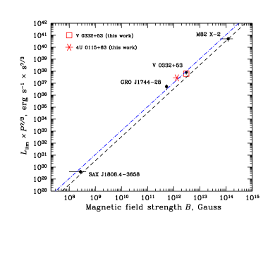
We also note, quite fundamentally, that accretion torque models generally assume an aligned rotator, while the spinning neutron stars in accreting binary pulsars are surely not aligned rotators. Unfortunately, 3D-calculations of magnetospheres, as done for T Tauri stars or CVs (see e.g., Romanova et al., 2008; Kulkarni & Romanova, 2013), have so far not been done for the geometrically much larger systems of neutron stars with terra-Gauss fields.
The above considerations make apparent that one should not take the observed cyclotron line energy and the derived field strength as a measure of the global dipole field and to calculate other system parameters like the distance – or even basic neutron star parameters like mass and radius – by applying an accretion torque model (as has been done in the literature, for example Takagi et al. 2016).
For completeness, we mention a third method to estimate the magnetic moment , based on flux and timing observations: when the mass accretion rate becomes very low, the magnetospheric radius increases, reaching and exceeding the co-rotation radius. Then the so called propeller effect (Illarionov & Sunyaev, 1975; Stella et al., 1986; Christodoulou et al., 2017) sets in, by which material at the inner edge of the accretion disk is thrown out by the rotating magnetic field (often referred to as “centrifugal barrier”), efficiently inhibiting accretion and leading to a dramatic drop (approximately two orders of magnitude) in X-ray luminosity. The onset of the “propeller effect” starts at a limiting accretion rate which can be calculated by equating the co-rotation radius Rc = (where the angular velocity of the magnetosphere equals that of the material in the Kepler orbit at the inner edge of the accretion disk) with the magnetospheric radius Rm = k . G is the gravitational constant, P the spin period, M the mass of the NS, the accretion rate, the magnetic moment of the NS and k a numerical factor (usually 0.5). The limiting accretion rate determines a limiting luminosity Llim (Campana et al., 2002; Fürst et al., 2017):
| (10) |
with quantities as defined above, plus R6 being the NS radius in units of cm, B12 being the polar magnetic field strength in units of Gauss (related to the magnetic moment = 0.5 BR3), being a numerical factor on the order of one. Tsygankov et al. (2016a, c) give an impressive example of five objects showing the “propeller effect”, which demonstrates that the relation LlimP7/3 B holds for 7 orders of magnitude in B (see Fig. 14). This method, however, does not have the power to resolve the above discussed differences between B-estimates through torque models and CRSF energies, since the systematic uncertainties are of similar magnitude.
7 Statistical analysis
Here we summarize some statistics regarding electron CRSF sources, numbers of sources showing specific characteristics.
-
•
350 known X-ray binary pulsars (XRBP) (e.g., Bildsten et al. 1997, or see footnotes202020http://www.iasf.inaf.it/m̃auro/pulsar_list.html#CRSF and 212121http://www.sternwarte.uni-erlangen.de/wiki/doku.php?id=xrp:start).
-
•
36 cyclotron line sources (10% of all XRBP) (see Table LABEL:tab:collection): 13 persistent High Mass X-ray Binaries (HMXB), 19 Be transients, 4 Low Mass X-ray Binaries (LMXB), plus 16 candidates) (see Table 4)
-
•
11 sources with multiple cyclotron lines (see Table LABEL:tab:collection):
7 sources with 2 lines; 3 sources with 3 lines (V 0332+53, MAXI J1409-619, GRO J1744-28), 1 source with more than 3 lines (4U 0115+63). -
•
7 sources with positive correlation of Ecyc with Lx (see Table 6): Her X-1, GX 304-1, Vela X-1, Cep X-4, V 0332+53, A 0535+26, 4U 1626.6-5156 (plus 4U 1907+09, to be confirmed).
-
•
2 sources with negative correlation of Ecyc with Lx (see Table 6): V 0332+53 (at very high Lx) and SMC X-2.
- •
-
•
18 sources with correlation of photon index with Lx (see Table 6).
8 Proton cyclotron lines
The resonances produced by protons gyrating in a strong magnetic field are lower in energy compared with those of electrons by a factor given by their mass ratio me/mp. Absorption lines seen by Chandra, XMM-Newton in the 0.2 10 keV band require very strong magnetic fields G. In contrast to electron cyclotron lines, those produced by protons (or nuclei) appear only at the fundamental frequency (Potekhin, 2010). The problem with proton line observations is that the absorption lines may be explained as well by other effects (Potekhin et al., 2015), for example by photo-ionisation in a dense cloud in the vicinity of the neutron star (Hambaryan et al., 2009), or as the result of a complex inhomogeneous temperature distribution on the surface of the neutron star (Viganò et al., 2014). The discovery of possible proton cyclotron lines has been reported for a number of objects (including ULXs and magnetars, which we do not discuss in detail here because of the problems of the just described confusion). We only mention the magnetar SGR 180620 (Ibrahim et al., 2002, 2003) for which the magnetic field strength estimated from P and is consistent with that inferred from an absorption line seen at 5 keV, assuming that it is a proton cyclotron line. The criterion also holds for a class of seven isolated neutron stars which were discovered in ROSAT data. They are bright X-ray sources but given their relatively small distances of typically a few hundred parsec they are intrinsically X-ray dim. Hence they are often called X-ray dim isolated neutron stars (XDINS) or simply the Magnificent Seven (M7). At least five of the seven objects exhibit absorption line features in the Chandra/XMM-Newton energy band (0.2-10 keV). When interpreted as proton cyclotron lines their corresponding magnetic field strengths agree with those derived from the measured P, data within a factor of a few (Haberl, 2007). In the following an update concerning these sources is given. In Sect. 8.1 we introduce the M7 stars and summarize their timing properties which help to constrain the large scale structure of their magnetic fields. The observed absorption features in their X-ray spectra are described in Sects. 8.2 and Sect. 8.3 the evidence for them being proton cyclotron lines is discussed, followed by a short summary. Fig. 15 shows an example of pulse phase resolved spectra of RX J0720.4-3125, with an absorption feature around 300 eV, as observed by XMM-Newton (Haberl, 2007).
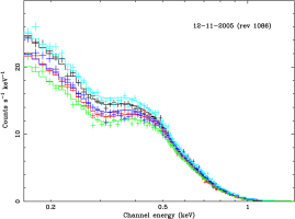
-
| Object | kT∞ | P | p.f.a𝑎aa𝑎aPulsed fraction. | Bdip | tkin | mBb𝑏bb𝑏bOptical magnitudes are taken from Kaplan (2008). | dc𝑐cc𝑐cDistance estimates indicated by are from Posselt et al. (2007). | Ref.d𝑑dd𝑑dReferences: (1) Haberl et al. (1999, 2004a); Kaplan & van Kerkwijk (2011) (2) Haberl et al. (1997); Cropper et al. (2001); Zane et al. (2002); de Vries et al. (2004); Haberl et al. (2004b); Kaplan & van Kerkwijk (2005a); Tetzlaff et al. (2011); Hohle et al. (2012b); Borghese et al. (2015); Hambaryan et al. (2017) (3) Haberl et al. (1998, 2004a); Kaplan & van Kerkwijk (2009a) (4) Schwope et al. (1999); Haberl et al. (2003); Kaplan & van Kerkwijk (2005b); Schwope et al. (2007); Tetzlaff et al. (2010); Hambaryan et al. (2011); Borghese et al. (2017) (5) Motch et al. (1999); van Kerkwijk et al. (2004); Motch et al. (2009); Tetzlaff et al. (2012); Pires et al. (2014, 2017) (6) Walter et al. (1996); Walter (2001); Burwitz et al. (2001, 2003); Tiengo & Mereghetti (2007); Walter et al. (2010); Tetzlaff et al. (2011); Mignani et al. (2013) (7) Zampieri et al. (2001); Zane et al. (2005); Kaplan & van Kerkwijk (2009b) | ||
|---|---|---|---|---|---|---|---|---|---|---|
| (eV) | (s) | (%) | (s s-1) | ( G) | (Myr) | (Myr) | (mag) | (pc) | ||
| RX J0420.0$-$5022 | 48 | 3.45 | 17 | 2.8 | 1.0 | 1.95 | ? | 26.6 | 345 | (1) |
| RX J0720.4$-$3125 | 8494 | 16.78 | 815 | 1.40 | 5.0 | 1.91 | 0.85 | 26.6 | 286 | (2) |
| RX J0806.4$-$4123 | 95 | 11.37 | 6 | 5.50 | 2.5 | 3.24 | ? | 24 | 250 | (3) |
| RX J1308.6+2127 | 100 | 10.31 | 18 | 1.12 | 3.5 | 1.45 | 0.55/0.90/1.38 | 28.4 | ? | (4) |
| RX J1605.3+3249 | 100 | ? | 2 | ? | ? | ? | 0.45 | 27.2 | 390 | (5) |
| RX J1856.5$-$3754 | 61 | 7.06 | 1 | 2.97 | 1.5 | 3.80 | 0.420.46 | 25.2 | 120 | (6) |
| RX J2143.0+0654 | 104 | 9.43 | 4 | 4.00 | 1.9 | 3.72 | ? | 26 | 430 | (7) |
8.1 The Magnificent Seven
RX J1856.53754 was the first isolated neutron star (INS) discovered in ROSAT data (Walter et al., 1996). Despite extensive searches only six further objects with similar properties, as summarized in Table 22, were found in the ROSAT data (Rutledge et al., 2003; Chieregato et al., 2005; Posselt et al., 2008; Agüeros et al., 2011). The X-ray emission of these seven objects is characterized by soft, blackbody-like emission attenuated by low photo-electric absorption by the interstellar medium, but in at least five cases with broad absorption features. The X-ray spectra show no indication of hard, non-thermal X-ray emission components which could originate from magneto-spheric activity. No flux variations on timescales of years are observed (but see RX J0720.43125 below), which suggests that we see thermal emission directly from the surface of cooling isolated neutron stars. Their distances range from 120 pc for RX J1856.53754 determined from parallax measurements (Walter et al., 2010) and several hundred pc constrained from absorption column densities (Posselt et al., 2007).
At least six of the M7 stars are X-ray pulsars with spin periods between 3.45 s (RX J0420.05022) and 16.78 s (RX J0720.43125). The modulation in the X-ray flux varies strongly from star to star with semi-amplitudes between 1% (RX J1856.53754) and 18% (RX J1308.6+2127). The latter shows a clear double-peaked pulse profile (Haberl et al., 2003), indicating a spin period of the NS twice as long as originally thought. The others are characterized by more gradual sinusoidal variations. Hambaryan et al. (2017) recently reported a double-hump pulse profile also for RX J0720.43125 (similar to RX J1308.6+2127), suggesting a spin period of 16.78 s. Spin down is observed from the M7 stars with known spin periods using a series of Chandra and XMM-Newton observations, with accurate spin-down rates obtained from coherent timing solutions. Assuming the model of magnetic dipole breaking (see also Sect. 6), the knowledge of the spin period P and its derivative allows one to estimate the magnetic field strength (B = 3.2; with B in Gauss, P in s and in s s-1), which yields values between 1 Gauss (RX J0420.05022) and 5.0 Gauss (RX J0720.43125). The characteristic ages estimated from the dipole model ( = P/(2)) of typically a few million years are a factor of a few longer than kinetic ages derived from back tracing the proper motion of the stars to likely birth places (Motch et al., 2009; Tetzlaff et al., 2010, 2011, 2012).
RX J0420.05022 was discovered serendipitously in ROSAT data (Haberl et al., 1999) as X-ray source with a soft blackbody-like spectrum and no optical counterpart (mB 25.25 mag). XMM-Newton observations with the EPIC-pn instrument revealed pulsations with a period of 3.45 s, the shortest confirmed spin period among the M7 stars (Haberl et al., 2004a). Using 14 observations with XMM-Newton Kaplan & van Kerkwijk (2011) obtained a phase-coherent timing solution and measured a spin-down rate of = (2.80.3) s s-1, which yields the lowest dipolar magnetic field strength of 1.0 G.
RX J0720.43125 is the second brightest M7 star discovered in ROSAT all-sky survey data and pulsations with a period of 8.39 s were indicated in the data of follow-up ROSAT PSPC and HRI pointed observations (Haberl et al., 1997). However, from a re-analysis of all available XMM-Newton high statistical quality data, Hambaryan et al. (2017) concluded that the true spin period is 16.74 s. The pulse profile folded at this period shows two humps with similar, but still clearly distinguishable shape. The object is unique as the only M7 star showing long-term variations in the X-ray spectrum on timescales of years (de Vries et al., 2004). A final analysis of monitoring observations with the EPIC-pn instrument of XMM-Newton spanning more than 11 years revealed a temperature increase from kT = 85 eV to 94 eV within about 1.5 yr. After reaching the maximum temperature, the spectra indicate a very slow cooling by 2 eV over 7 yr (Hohle et al., 2012b).
RX J0806.44123 was discovered in a dedicated search for INS in the ROSAT all-sky survey (Haberl et al., 1998). The spin period of 11.37 s was detected in XMM-Newton data (Haberl & Zavlin, 2002) and the period derivative could be constrained from a series of follow-up observations, although with large uncertainties (Kaplan & van Kerkwijk, 2009a).
RX J1308.6+2127 = RBS 1223 was identified as source with empty error circle in the ROSAT Bright Survey (RBS) catalog (Schwope et al., 1999, 2000). Follow-up Chandra observations first suggested a period of 5.16 s (Hambaryan et al., 2002) before XMM-Newton observations provided data of high statistical quality which revealed a double-peak pulse profile with true period of 10.31 s (Haberl et al., 2003). A coherent timing solution was obtained from Chandra and XMM-Newton observations spanning a period of five years, yielding accurate values for spin period and derivative (Kaplan & van Kerkwijk, 2005b).
RX J1605.3+3249 = RBS 1556 was selected as INS from the ROSAT all-sky survey on the basis of its spectral softness and lack of bright optical counterpart (Motch et al., 1999). An indication for a spin period (3.39 s) was reported at a 4 confidence level together with uncertain constraints for the pulsar spin-down rate (Pires et al., 2014). However, using recent deep XMM-Newton observations Pires et al. (2017) could not confirm the period with upper limits for the pulsed fraction of 2.6%.
RX J1856.53754 is the X-ray brightest M7 star and was first found in a ROSAT pointed PSPC observation as brightest source in the field of view (Walter et al., 1996). Together with the ROSAT all-sky survey detection and a ROSAT HRI observation no evidence for variability was found and the limit for F/Fopt of 7000 strongly suggested an INS nature of the object. This first discovery triggered the search for other sources in the ROSAT all-sky survey with similar properties. The ROSAT PSPC spectrum could be modeled by pure blackbody emission and also the high-resolution Chandra LETG spectra did not reveal any significant deviations from a Planckian energy distribution (Burwitz et al., 2001, 2003). Although being the brightest M7 star, no absorption feature similar to those found in other M7 stars was significantly detected so far. A very shallow modulation (1%) with a period of 7.06 s was discovered in XMM-Newton EPIC-pn data (Tiengo & Mereghetti, 2007) and constraints on the period derivative indicate a magnetic field strength comparable to what was found for the other M7 (van Kerkwijk & Kaplan, 2008).
RX J2143.0+0654 = 1RXS J214303.7+065419 = RBS 1774 was the last of the M7 discovered in ROSAT data (Zampieri et al., 2001). Again XMM-Newton observations led to the discovery of X-ray pulsations (period 9.437 s) and an absorption feature at 700–750 eV (Zane et al., 2005; Cropper et al., 2007). From an additional series of XMM-Newton observations Kaplan & van Kerkwijk (2009b) measured the spin-down rate, which indicates a magnetic dipole field strength of 2 G.
| Object | ———————– Broad lines ———————– | ——— Narrow lines ——— | ||||
|---|---|---|---|---|---|---|
| Ecyc | eqwcyca𝑎aa𝑎aEquivalent width of broad absorption line. Numbers in parentheses indicate variations with pulse phase. | Bcyc | Ecyc | eqwcyc | Bcyc | |
| (eV) | (eV) | ( G) | (eV) | (eV) | ( G) | |
| RX J0420.0$-$5022b𝑏bb𝑏bLine parameters subject to possible large systematic uncertainties (see text). | 329:c𝑐cc𝑐cThe colon indicates that the parameters are subject to larger calibration uncertainties (see text). | 43: | 6.5: | |||
| RX J0720.4$-$3125 | 300 | 10 to 75 (20) | 6.0 | 750 | 30 | 14.9 |
| RX J0806.4$-$4123 | 410-490 | 45 | 8.1-9.7 | |||
| RX J1308.6+2127 | 300 | 150 (20) | 6.0 | 750 | 15 | 14.9 |
| RX J1605.3+3249 | 443/828 | 31/13 | 8.8/16.4 | |||
| RX J1856.5$-$3754 | 250 or 800 | ? | 5.0 or 15.9 | |||
| RX J2143.0+0654 | 750 | 25 | 14.9 | |||
8.2 Proton absorption features
The ROSAT PSPC spectra of the M7 were modeled with blackbody emission attenuated by small amounts of absorption, which is interpreted to be induced by the interstellar medium. The energy resolution of the PSPC was not sufficient to discern additional absorption features. Moreover, the entrance window of the detector caused a deep carbon absorption edge with strong depression of the effective area between 300 eV and 500 eV, the energy band in which features were later found in the XMM-Newton and Chandra spectra. The line properties are described in the following and summarized in Table 23.
The first absorption feature was discovered by Haberl et al. (2003) in data collected from RX J1308.6+2127 by the EPIC-pn instrument of XMM-Newton. The X-ray spectra show strong deviations from a Planckian energy distribution at energies below 500 eV which can be modeled by a Gaussian-shaped absorption line centered at an energy of 300 eV and with width of 100 eV, although even broader lines at energies down to 100 eV or several unresolved lines can not be excluded. The depth of the line relative to the continuum (the equivalent width, eqw) was measured to 150 eV (we use negative values to indicate that the line is in absorption), the deepest absorption line seen from the M7. Moreover, pulse-phase spectroscopy revealed the line to vary in strength with a full amplitude of 40 eV in equivalent width (Schwope et al., 2005). The line is deepest at the intensity maxima of the double-peaked pulse profile and shallowest at the minima.
A similar behavior was found for RX J0720.43125. Haberl et al. (2004b) reported a phase-dependent absorption line in the spectrum which varies in depth with pulse phase. This line is broad (64 eV 1 width when modeled with a Gaussian profile) and centered at 300 eV (Haberl et al., 2004b, 2006). The equivalent width varies with pulse phase from 31 eV around intensity maximum and 58 eV at the declining part of the pulse. While the line is much weaker on average, the full amplitude variation with pulse phase is almost as large as for RX J1308.6+2127. Additionally, the line depth was found to change on timescales of years. Parallel to the increase in temperature with a maximum seen in May 2004 the line depth also increased from eqw = 40 eV to 74 eV in the phase-averaged spectra (Haberl et al., 2006; Hohle et al., 2012b). It is remarkable that the amplitude in the variations with pulse phase stayed constant at 40 eV (Hohle et al., 2009).
While for RX J1308.6+2127 and RX J0720.43125 the variability of the absorption lines with pulse-phase excludes all possible doubt that they are real spectral features, the detection of a broad absorption line in the high resolution X-ray spectra of RX J1605.3+3249 obtained by the RGS instruments of XMM-Newton constrains the width of the line. Relative to CCD detectors, the superior energy resolution of the RGS revealed that the deviation from a blackbody spectrum can be well modeled with a single broad absorption line centered at 450 eV with a 1 width of 59 eV (van Kerkwijk et al., 2004). On the other hand, the high statistical quality of the EPIC-pn spectra of RX J1605.3+3249 revealed strong evidence for the existence of multiple lines. An acceptable fit was only reached when including three Gaussian absorption lines at energies of E1 = 4032 eV, E2 = 5894 eV and E3 = 78024 (Haberl, 2007). It is remarkable that the ratios of the line energies are consistent with 1:1.5:2. The existing data at the time of that work did not allow the fitting of the width of the lines individually and a single common fit parameter was derived with of 87 eV. Including the spectra from new XMM-Newton observations required an even more complex modeling with two blackbody components for the continuum (a cool one with kT around 30 eV and the dominant hot one with kT 110 eV) and three absorption lines (Pires et al., 2014). From RGS spectra these authors determined E1 = 443 eV ( = 74 eV and eqw = 31 eV) and E2 = 8285 eV ( = 15 +/-4 eV and eqw 13 eV). A somewhat narrower line with central energy of E = 5768 eV and Gaussian width = 16 eV (eqw = 5 eV) was already reported by van Kerkwijk et al. (2004) and might be explained by the presence of highly ionized oxygen (O VII) in the interstellar medium and/or absorption in the neutron star atmosphere by O VIII, gravitationally red-shifted (Hohle et al., 2012a). A narrow line at similar energy (569 eV) was also reported from RX J0720.43125 (Hambaryan et al., 2009; Hohle et al., 2012a) and at 535 eV from RX J1308.6+2127 (Hohle et al., 2012a). The new RGS results for the lines at 576 eV and 828 eV makes it less clear if they are related to the broad absorption feature at 440 eV.
The properties of absorption features in the spectra of RX J2143.0+0654 and RX J0806.44123 are less clear. A feature found in the first XMM-Newton observation of RX J2143.0+0654 was reported by Zane et al. (2005) at an energy of 700 eV (when modeled with an absorption edge) or 750 eV (multiplicative Gaussian line). New XMM-Newton observations with a factor of 2.5 more exposure confirmed this and Kaplan & van Kerkwijk (2009b) inferred a significant improvement in fit quality when including a multiplicative Gaussian line with a width of 73 eV, centered at 756 eV in the spectral model. This is the highest energy measured for an M7 star and yields a magnetic field strength more than a factor of seven higher than the field strength inferred from the dipole model, while for the other M7 stars this factor is more typical 1.2 to 4. Also for RX J0806.44123 the spectral modeling is formally improved when considering an absorption line. Fixing the width of the line at 70 eV, Haberl et al. (2004a) derive line parameters of 46015 eV for the central line energy and eqw = 336 eV from the merged EPIC-pn spectrum of two XMM-Newton observations. For the corresponding RGS spectra the authors report 41319 eV and 5613 eV, respectively. With the errors at 90% confidence level, the parameters are formally inconsistent and indicate large systematic uncertainties. Moreover, Kaplan & van Kerkwijk (2009a) report a line energy of 4865 eV from EPIC-pn observations performed in 2008 and 2009 (a factor of four more exposure than available from the older observations). These authors also find further improvement in fit quality when using two Gaussian lines (E1 = 4605 eV, eqw1 = 89 eV, E2 = 69312 eV, eqw2 = 55 eV). It should be noted that they also fix all line widths at the same value (85 eV) while experience with RX J1605.3+3249 shows that they can be considerably different.
RX J0420.05022 is the X-ray faintest of the M7 and exhibits the softest spectrum, which makes it difficult to confirm
the existence of absorption features due to possible systematic calibration uncertainties caused by insufficient energy
resolution at low energies (300 eV) in modern CCD detectors. Formally, the fit to the EPIC-pn phase-averaged
spectra improves when a Gaussian absorption line is added to the absorbed blackbody model (Haberl et al., 2004a).
Because the line parameters are subject to larger calibration uncertainties, we list them in Table 23 with colon.
The discovery of a second strongly phase-variable narrow absorption feature at 750 eV was recently reported for RX J0720.43125 and RX J1308.6+2127 (Borghese et al., 2015, 2017). The fact that the features are significantly detected for only 20% of the pulsar rotation suggests that they are formed very close to the neutron star’s surface.
8.3 Origin of proton cyclotron lines
The absence of non-thermal emission components in the X-ray spectra of the M7, no confirmed radio detection and their insufficient spin-down energy losses to power the X-ray emission lead to the generally accepted picture of cooling isolated neutron stars. The M7 provide the unique opportunity to obtain information about their magnetic fields in two independent ways. One method is based on the measurement of the spin down rate and assumes magnetic dipole breaking according to the model of a magnetic dipole rotating in vacuum. A more direct determination of the magnetic field strength is possible when cyclotron resonance lines can be observed in the X-ray spectra. Unlike for accreting X-ray pulsars the absorption features observed from M7 stars can not be caused by electrons because the inferred magnetic field strength is by far incompatible with that derived from magnetic dipole breaking. For protons the derived field strengths are generally higher but more consistent with the dipole model. However: which particles contribute, is also a matter of the composition of the neutron star atmosphere. Moreover, bound-bound and bound-free transitions of neutral hydrogen are also expected at similar energies for magnetic fields above 1013 G (see Fig. 7 in van Kerkwijk & Kaplan, 2007).
However, whether or not transitions of free protons or magnetized hydrogen atoms contribute to the observed lines, is a matter of the temperature distribution in the neutron star atmosphere. According to Fig. 1 in Ho et al. (2003) the atomic fraction of hydrogen at temperatures of kT = 50 100 eV typical for the M7 is rather low (=0.3 %). As a consequence the proton cyclotron lines dominate the spectrum (Figs. 2 and 3 of Ho et al., 2003), while atomic hydrogen transitions may produce additional features. That may explain some of the observed multiple lines. In view of the limited significance of the line detections it appears difficult to make specific assignments.
Another way to explain multiple lines is to invoke – beyond the radiation from the hot cap at the magnetic dipole – separate hot spots on the stellar surface having higher multipolar magnetic fields. The first strong evidence for this comes from the discovery of strongly phase-variable absorption lines which are visible only for about 20% of the neutron star rotation. The lines were detected in the X-ray spectra of RX J0720.43125 and RX J1308.6+2127 (Borghese et al., 2015, 2017, respectively) and have energies a factor of 2.5 higher than the broad lines (Table 23). Such multipole fields must be quite young compared to the age of the NS. They may be formed by extracting magnetic energy from the toroidal field that resides in deep crustal layers, via Hall drift (e.g., Geppert & Viganò, 2014).
We conclude that proton cyclotron lines produced in strong magnetic fields of isolated neutron stars can explain the absorption-type features observed in the soft X-ray spectra of young isolated neutron stars of the M7 class. More accurate measurements in the future in combination with further theoretical work on magnetized atmospheres and the magneto-thermal evolution of neutron stars are required to make further progress in this exciting field.
9 Summary
With this contribution we attempt to provide a review on the current state of our knowledge about X-ray sources that show cyclotron line features in their spectra – both for electron cyclotron lines (this is by far the larger part) and for proton cyclotron lines. We concentrate on the observational aspects, providing a number of Tables that contain detailed informations on all sources that we consider reasonably well secured regarding the existence of cyclotron lines. In the case of electron cyclotron lines – observed from binary X-ray pulsars, highly magnetized accreting neutron stars in binaries – we also give a Table with candidate sources, mostly objects for which a detection of a cyclotron line was claimed some time ago, but had not been confirmed in subsequent observations, or sources that were observed rather recently, but only once and with somewhat peculiar properties. On the other hand: for some of the objects listed in the main Tables, the existence of a cyclotron line still needs confirmation (or not) through re-measurements (with a finite probability that they have to be moved into the candidates category). We try to address the basic physics underlying the cyclotron line phenomenon, including a large number of references to theoretical work, with some coverage of specific theoretical modeling.
Since the discovery of the first CRSF in Her X-1 in 1976, a new field of Cyclotron Line Research has evolved. With the rather fast confirmation of the line in Her X-1 after 1977 by a number of different instruments and the detection of the same phenomenon in other X-ray binary pulsars, an impressive wave of theoretical work was initiated, leading to a basic understanding of the underlying physics. Observational activities have lead to the discovery of many more objects until today (at an approximate mean rate of one per year). In the meantime the emphasis has, however, shifted from a pure discovery of new cyclotron line objects to the investigation of physical details like the width, depth, line profile, phase dependence, etc., of the lines and to new associated phenomena like the dependence of the cyclotron line energy on luminosity or its long-term decay (so far found in only two sources). This has been possible through modern instruments (like NuSTAR), with good energy resolution, broad spectral coverage and low background and high sensitivity. On the theoretical front, progress has been made in the understanding and modeling of the phenomenon, leading for example, to a procedure to fit observed spectra to theoretical spectra that are generated by highly complex Monte Carlo modeling, allowing us to find solid physical parameters. Overall, however, our feeling is that theoretical work is somewhat lagging behind observations, and that there are many open questions to be answered.
Acknowledgements.
We thank the anonymous referee for very useful comments that allowed us to improve the text.References
- Agüeros et al. (2011) Agüeros, M. A., Posselt, B., Anderson, S. F., et al. 2011, AJ, 141, 176
- Alford & Halpern (2016) Alford, J. A. J. & Halpern, J. P. 2016, ApJ, 818, 122
- Antoniou et al. (2018) Antoniou, V., Zezas, A., Hong, J., et al. 2018, The Astronomer’s Telegram, 12234
- Araya & Harding (1999) Araya, R. & Harding, A. 1999, ApJ, 517, 334
- Araya-Góchez & Harding (2000) Araya-Góchez, R. A. & Harding, A. K. 2000, ApJ, 544, 1067
- Argyle et al. (1983) Argyle, R. W., Eldridge, P., King, D. L., Honeycutt, R. K., & Schlegel, E. M. 1983, IAU Circ., 3899
- Arons et al. (1987) Arons, J., Klein, R. I., & Lea, S. M. 1987, ApJ, 312, 666
- Augello et al. (2003) Augello, G., Iaria, R., Robba, N. R., et al. 2003, ApJ, 596, L63
- Bailer-Jones et al. (2018) Bailer-Jones, C. A. L., Rybizki, J., Fouesneau, M., Mantelet, G., & Andrae, R. 2018, AJ, 156, 58
- Ballhausen et al. (2016) Ballhausen, R., Kühnel, M., Pottschmidt, K., et al. 2016, A&A, 591, A65
- Ballhausen et al. (2017) Ballhausen, R., Pottschmidt, K., Fürst, F., et al. 2017, A&A, 608, A105
- Barnstedt et al. (2008) Barnstedt, J., Staubert, R., Santangelo, A., et al. 2008, A&A, 486, 293
- Basko & Sunyaev (1975) Basko, M. M. & Sunyaev, R. A. 1975, A&A, 42, 311
- Basko & Sunyaev (1976) Basko, M. M. & Sunyaev, R. A. 1976, MNRAS, 175, 395
- Baykal et al. (2010) Baykal, A., Göǧüş, E., Çaǧdaş İnam, S., & Belloni, T. 2010, ApJ, 711, 1306
- Baykal et al. (2007) Baykal, A., Inam, S. Ç., Stark, M. J., et al. 2007, MNRAS, 374, 1108
- Baykal et al. (2000) Baykal, A., Stark, M. J., & Swank, J. 2000, ApJ, 544, L129
- Becker et al. (2012) Becker, P. A., Klochkov, D., Schönherr, G., et al. 2012, A&A, 544, A123
- Becker & Wolff (2007) Becker, P. A. & Wolff, M. T. 2007, ApJ, 654, 435
- Bellm et al. (2014) Bellm, E. C., Fürst, F., Pottschmidt, K., et al. 2014, ApJ, 792, 108
- Bhalerao et al. (2015) Bhalerao, V., Romano, P., Tomsick, J., et al. 2015, MNRAS, 447, 2274
- Bildsten et al. (1997) Bildsten, L., Chakrabarty, D., Chiu, J., et al. 1997, ApJS, 113, 367
- Bisnovatyi-Kogan & Fridman (1970) Bisnovatyi-Kogan, G. S. & Fridman, A. M. 1970, Sov. Ast., 13, 566
- Blay et al. (2006) Blay, P., Negueruela, I., Reig, P., et al. 2006, A&A, 446, 1095
- Blay et al. (2005) Blay, P., Ribó, M., Negueruela, I., et al. 2005, A&A, 438, 963
- Bodaghee et al. (2016) Bodaghee, A., Tomsick, J. A., Fornasini, F. M., et al. 2016, ApJ, 823, 146
- Bodaghee et al. (2006) Bodaghee, A., Walter, R., Zurita Heras, J. A., et al. 2006, A&A, 447, 1027
- Boldin et al. (2013) Boldin, P. A., Tsygankov, S. S., & Lutovinov, A. A. 2013, Astronomy Letters, 39, 375
- Bonazzola et al. (1979) Bonazzola, S., Heyvaerts, J., & Puget, J. L. 1979, A&A, 78, 53
- Bonnet-Bidaud & Mouchet (1998) Bonnet-Bidaud, J. M. & Mouchet, M. 1998, A&A, 332, L9
- Bonning & Falanga (2005) Bonning, E. W. & Falanga, M. 2005, A&A, 436, L31
- Borghese et al. (2015) Borghese, A., Rea, N., Coti Zelati, F., Tiengo, A., & Turolla, R. 2015, ApJ, 807, L20
- Borghese et al. (2017) Borghese, A., Rea, N., Coti Zelati, F., et al. 2017, MNRAS, 468, 2975
- Bozzo et al. (2011) Bozzo, E., Ferrigno, C., Falanga, M., & Walter, R. 2011, A&A, 531, A65
- Braun & Yahel (1984) Braun, A. & Yahel, R. Z. 1984, ApJ, 278, 349
- Brightman et al. (2018) Brightman, M., Harrison, F. A., Fürst, F., et al. 2018, Nature Astronomy, 2, 312
- Brumback et al. (2018) Brumback, M. C., Hickox, R. C., Fürst, F. S., et al. 2018, ApJ, 852, 132
- Burderi et al. (2000) Burderi, L., Di Salvo, T., Robba, N. R., La Barbera, A., & Guainazzi, M. 2000, ApJ, 530, 429
- Burnard et al. (1991) Burnard, D. J., Arons, J., & Klein, R. I. 1991, ApJ, 367, 575
- Burwitz et al. (2003) Burwitz, V., Haberl, F., Neuhäuser, R., et al. 2003, A&A, 399, 1109
- Burwitz et al. (2001) Burwitz, V., Zavlin, V. E., Neuhäuser, R., et al. 2001, A&A, 379, L35
- Bussard (1980) Bussard, R. W. 1980, ApJ, 237, 970
- Bykov & Krasil’shchikov (2004) Bykov, A. M. & Krasil’shchikov, A. M. 2004, Astronomy Letters, 30, 309
- Caballero et al. (2007) Caballero, I., Kretschmar, P., Santangelo, A., et al. 2007, A&A, 465, L21
- Caballero et al. (2013a) Caballero, I., Kühnel, M., Pottschmidt, K., et al. 2013a, in AAS/High Energy Astrophysics Division, Vol. 13, AAS/High Energy Astrophysics Division, 126.32
- Caballero et al. (2013b) Caballero, I., Pottschmidt, K., Marcu, D. M., et al. 2013b, ApJ, 764, L23
- Caballero et al. (2008) Caballero, I., Santangelo, A., Kretschmar, P., et al. 2008, A&A, 480, L17
- Caballero & Wilms (2012) Caballero, I. & Wilms, J. 2012, Mem. Soc. Astron. Italiana, 83, 230
- Caballero-García et al. (2016) Caballero-García, M. D., Camero-Arranz, A., Özbey Arabacı, M., et al. 2016, A&A, 589, A9
- Camero-Arranz et al. (2012a) Camero-Arranz, A., Finger, M. H., Wilson-Hodge, C. A., et al. 2012a, ApJ, 754, 20
- Camero-Arranz et al. (2012b) Camero-Arranz, A., Pottschmidt, K., Finger, M. H., et al. 2012b, A&A, 546, A40
- Campana et al. (2002) Campana, S., Stella, L., Israel, G. L., et al. 2002, ApJ, 580, 389
- Carpano et al. (2018) Carpano, S., Haberl, F., Maitra, C., & Vasilopoulos, G. 2018, MNRAS, 476, L45
- Chieregato et al. (2005) Chieregato, M., Campana, S., Treves, A., et al. 2005, A&A, 444, 69
- Chodil et al. (1967) Chodil, G., Mark, H., Rodrigues, R., Seward, F. D., & Swift, C. D. 1967, ApJ, 150, 57
- Chou et al. (2016) Chou, Y., Hsieh, H.-E., Hu, C.-P., Yang, T.-C., & Su, Y.-H. 2016, ApJ, 831, 29
- Christodoulou et al. (2017) Christodoulou, D. M., Laycock, S. G. T., Yang, J., & Fingerman, S. 2017, Research in Astronomy and Astrophysics, 17, 059
- Clark et al. (1978) Clark, G., Doxsey, R., Li, F., Jernigan, J. G., & van Paradijs, J. 1978, ApJ, 221, L37
- Clark et al. (1979) Clark, G., Li, F., & van Paradijs, J. 1979, ApJ, 227, 54
- Clark et al. (1990) Clark, G. W., Woo, J. W., Nagase, F., Makishima, K., & Sakao, T. 1990, ApJ, 353, 274
- Coburn et al. (2001) Coburn, W., Heindl, W. A., Gruber, D. E., et al. 2001, ApJ, 552, 738
- Coburn et al. (2002) Coburn, W., Heindl, W. A., Rothschild, R. E., et al. 2002, ApJ, 580, 394
- Coburn et al. (2006) Coburn, W., Pottschmidt, K., Rothschild, R., et al. 2006, in Bulletin of the American Astronomical Society, Vol. 38, AAS/High Energy Astrophysics Division #9, 340
- Coe et al. (2007) Coe, M. J., Bird, A. J., Hill, A. B., et al. 2007, MNRAS, 378, 1427
- Cominsky et al. (1978) Cominsky, L., Clark, G. W., Li, F., Mayer, W., & Rappaport, S. 1978, Nature, 273, 367
- Corbet et al. (1986) Corbet, R. H. D., Charles, P. A., & van der Klis, M. 1986, A&A, 162, 117
- Corbet et al. (2018) Corbet, R. H. D., Coley, J. B. C., Krim, H. A., & Pottschmidt, K. 2018, The Astronomer’s Telegram 11918
- Corbet & Krimm (2009) Corbet, R. H. D. & Krimm, H. A. 2009, The Astronomer’s Telegram, 2008
- Corbet et al. (2010a) Corbet, R. H. D., Krimm, H. A., Barthelmy, S. D., et al. 2010a, The Astronomer’s Telegram, 2570
- Corbet et al. (2007) Corbet, R. H. D., Markwardt, C. B., & Tueller, J. 2007, ApJ, 655, 458
- Corbet et al. (2001) Corbet, R. H. D., Marshall, F. E., Coe, M. J., Laycock, S., & Handler, G. 2001, ApJ, 548, L41
- Corbet et al. (2010b) Corbet, R. H. D., Pearlman, A. B., & Pottschmidt, K. 2010b, The Astronomer’s Telegram, 2766
- Crampton et al. (1978) Crampton, D., Hutchings, J. B., & Cowley, A. P. 1978, ApJ, 223, L79
- Crampton et al. (1985) Crampton, D., Hutchings, J. B., & Cowley, A. P. 1985, ApJ, 299, 839
- Cropper et al. (2001) Cropper, M., Zane, S., Ramsay, G., Haberl, F., & Motch, C. 2001, A&A, 365, L302
- Cropper et al. (2007) Cropper, M., Zane, S., Turolla, R., et al. 2007, Ap&SS, 308, 161
- Cusumano et al. (2016) Cusumano, G., La Parola, V., D’Aì, A., et al. 2016, MNRAS, 460, L99
- Cusumano et al. (2010) Cusumano, G., La Parola, V., Romano, P., et al. 2010, MNRAS, 406, L16
- D’Aì et al. (2017) D’Aì, A., Cusumano, G., Del Santo, M., La Parola, V., & Segreto, A. 2017, MNRAS, 470, 2457
- D’Aì et al. (2011) D’Aì, A., Cusumano, G., La Parola, V., et al. 2011, A&A, 532, A73
- D’Aì et al. (2015) D’Aì, A., Di Salvo, T., Iaria, R., et al. 2015, MNRAS, 449, 4288
- Dal Fiume et al. (1998) Dal Fiume, D., Orlandini, M., Cusumano, G., et al. 1998, A&A, 329, L41
- dal Fiume et al. (2000) dal Fiume, D., Orlandini, M., del Sordo, S., et al. 2000, in Broad Band X-ray Spectra of Cosmic Sources, ed. K. Makishima, L. Piro, & T. Takahashi, 399
- Daugherty & Ventura (1977) Daugherty, J. K. & Ventura, J. 1977, A&A, 61, 723
- Davidson (1973) Davidson, K. 1973, Nature Physical Science, 246, 1
- de Vries et al. (2004) de Vries, C. P., Vink, J., Méndez, M., & Verbunt, F. 2004, A&A, 415, L31
- DeCesar et al. (2013) DeCesar, M. E., Boyd, P. T., Pottschmidt, K., et al. 2013, ApJ, 762, 61
- Degenaar et al. (2014) Degenaar, N., Miller, J. M., Harrison, F. A., et al. 2014, ApJ, 796, L9
- den Hartog et al. (2006) den Hartog, P. R., Hermsen, W., Kuiper, L., et al. 2006, A&A, 451, 587
- Doroshenko (2017) Doroshenko, A. 2017, private comm., 1, yyy
- Doroshenko (2017) Doroshenko, R. 2017, PhD thesis, Univ. of Tübingen
- Doroshenko et al. (2015) Doroshenko, R., Santangelo, A., Doroshenko, V., Suleimanov, V., & Piraino, S. 2015, MNRAS, 452, 2490
- Doroshenko et al. (2012) Doroshenko, V., Santangelo, A., Kreykenbohm, I., & Doroshenko, R. 2012, A&A, 540, L1
- Doroshenko et al. (2010) Doroshenko, V., Suchy, S., Santangelo, A., et al. 2010, A&A, 515, L1
- Doroshenko et al. (2017) Doroshenko, V., Tsygankov, S. S., Mushtukov, A. A., et al. 2017, MNRAS, 466, 2143
- Enoto et al. (2008) Enoto, T., Makishima, K., Terada, Y., et al. 2008, PASJ, 60, 57
- Epili et al. (2016) Epili, P., Naik, S., & Jaisawal, G. K. 2016, Research in Astronomy and Astrophysics, 16, 77
- Falkner et al. (2018) Falkner, S., Schwarm, F.-W., Dauser, T., & et al. 2018, submitted
- Farinelli et al. (2012) Farinelli, R., Ceccobello, C., Romano, P., & Titarchuk, L. 2012, A&A, 538, A67
- Farinelli et al. (2016) Farinelli, R., Ferrigno, C., Bozzo, E., & Becker, P. A. 2016, A&A, 591, A29
- Farrell et al. (2006) Farrell, S. A., Sood, R. K., & O’Neill, P. M. 2006, MNRAS, 367, 1457
- Farrell et al. (2008) Farrell, S. A., Sood, R. K., O’Neill, P. M., & Dieters, S. 2008, MNRAS, 389, 608
- Ferrigno et al. (2009) Ferrigno, C., Becker, P. A., Segreto, A., Mineo, T., & Santangelo, A. 2009, A&A, 498, 825
- Ferrigno et al. (2016a) Ferrigno, C., Ducci, L., Bozzo, E., et al. 2016a, A&A, 595, A17
- Ferrigno et al. (2011) Ferrigno, C., Falanga, M., Bozzo, E., et al. 2011, A&A, 532, A76
- Ferrigno et al. (2013) Ferrigno, C., Farinelli, R., Bozzo, E., et al. 2013, A&A, 553, A103
- Ferrigno et al. (2016b) Ferrigno, C., Pjanka, P., Bozzo, E., et al. 2016b, A&A, 593, A105
- Ferrigno et al. (2007) Ferrigno, C., Segreto, A., Santangelo, A., et al. 2007, A&A, 462, 995
- Finger et al. (1996) Finger, M. H., Wilson, R. B., & Harmon, B. A. 1996, ApJ, 459, 288
- Freeman et al. (1996) Freeman, P. et al. 1996, in Gamma Ray Bursts, Proc. 3rd Huntsville Symp., ed. Koveliotou/Briggs/Fishman, 172
- Fuerst et al. (2018) Fuerst, F., Falkner, S., Marcu-Cheatham, D., et al. 2018, ArXiv:1809.05691 [arXiv:1809.05691:1809.05691]
- Fürst et al. (2013) Fürst, F., Grefenstette, B. W., Staubert, R., et al. 2013, ApJ, 779, 69
- Fürst et al. (2017) Fürst, F., Kretschmar, P., Kajava, J. J. E., et al. 2017, A&A, 606, A89
- Fürst et al. (2011) Fürst, F., Kreykenbohm, I., Suchy, S., et al. 2011, A&A, 525, A73
- Fürst et al. (2012) Fürst, F., Pottschmidt, K., Kreykenbohm, I., et al. 2012, A&A, 547, A2
- Fürst et al. (2015) Fürst, F., Pottschmidt, K., Miyasaka, H., et al. 2015, ApJ, 806, L24
- Fürst et al. (2014a) Fürst, F., Pottschmidt, K., Wilms, J., et al. 2014a, ApJ, 784, L40
- Fürst et al. (2014b) Fürst, F., Pottschmidt, K., Wilms, J., et al. 2014b, ApJ, 780, 133
- Galloway et al. (2005) Galloway, D. K., Wang, Z., & Morgan, E. H. 2005, ApJ, 635, 1217
- Geppert & Viganò (2014) Geppert, U. & Viganò, D. 2014, MNRAS, 444, 3198
- Ghosh & Lamb (1979a) Ghosh, P. & Lamb, F. K. 1979a, ApJ, 232, 259
- Ghosh & Lamb (1979b) Ghosh, P. & Lamb, F. K. 1979b, ApJ, 234, 296
- Ghosh et al. (1977) Ghosh, P., Lamb, F. K., & Pethick, C. J. 1977, ApJ, 217, 578
- Giacconi et al. (1972) Giacconi, R., Murray, S., Gursky, H., et al. 1972, ApJ, 178, 281
- Giangrande et al. (1980) Giangrande, A., Giovannelli, F., Bartolini, C., Guarnieri, A., & Piccioni, A. 1980, A&AS, 40, 289
- Gnedin & Sunyaev (1974) Gnedin, I. N. & Sunyaev, R. A. 1974, A&A, 36, 379
- Gold (1968) Gold, T. 1968, Nature, 218, 731
- Goldreich & Julian (1969) Goldreich, P. & Julian, W. H. 1969, ApJ, 157, 869
- Grove et al. (1995) Grove, J. E., Strickman, M. S., Johnson, W. N., et al. 1995, ApJ, 438, L25
- Gruber et al. (2001) Gruber, D. E., Heindl, W. A., Rothschild, R. E., et al. 2001, ApJ, 562, 499
- Gruber et al. (1999) Gruber, D. E., Heindl, W. A., Rothschild, R. E., et al. 1999, in Highlights in X-ray Astronomy, ed. B. Aschenbach & M. J. Freyberg, Vol. 272, 33
- Gruber et al. (1980) Gruber, D. E., Matteson, J. L., Nolan, P. L., & et al. 1980, ApJ, 240, L127
- Haberl (2007) Haberl, F. 2007, Ap&SS, 308, 181
- Haberl et al. (1997) Haberl, F., Motch, C., Buckley, D. A. H., Zickgraf, F.-J., & Pietsch, W. 1997, A&A, 326, 662
- Haberl et al. (1998) Haberl, F., Motch, C., & Pietsch, W. 1998, Astronomische Nachrichten, 319, 97
- Haberl et al. (2004a) Haberl, F., Motch, C., Zavlin, V. E., et al. 2004a, A&A, 424, 635
- Haberl et al. (1999) Haberl, F., Pietsch, W., & Motch, C. 1999, A&A, 351, L53
- Haberl et al. (2003) Haberl, F., Schwope, A. D., Hambaryan, V., Hasinger, G., & Motch, C. 2003, A&A, 403, L19
- Haberl et al. (2006) Haberl, F., Turolla, R., de Vries, C. P., et al. 2006, A&A, 451, L17
- Haberl & Zavlin (2002) Haberl, F. & Zavlin, V. E. 2002, A&A, 391, 571
- Haberl et al. (2004b) Haberl, F., Zavlin, V. E., Trümper, J., & Burwitz, V. 2004b, A&A, 419, 1077
- Haigh et al. (2004) Haigh, N. J., Coe, M. J., & Fabregat, J. 2004, MNRAS, 350, 1457
- Halpern (2012) Halpern, J. P. 2012, The Astronomer’s Telegram, 3949
- Halpern & Gotthelf (2007) Halpern, J. P. & Gotthelf, E. V. 2007, ApJ, 669, 579
- Hambaryan et al. (2002) Hambaryan, V., Hasinger, G., Schwope, A. D., & Schulz, N. S. 2002, A&A, 381, 98
- Hambaryan et al. (2009) Hambaryan, V., Neuhäuser, R., Haberl, F., Hohle, M. M., & Schwope, A. D. 2009, A&A, 497, L9
- Hambaryan et al. (2017) Hambaryan, V., Suleimanov, V., Haberl, F., et al. 2017, A&A, 601, A108
- Hambaryan et al. (2011) Hambaryan, V., Suleimanov, V., Schwope, A. D., et al. 2011, A&A, 534, A74
- Heindl et al. (2003) Heindl, W., Coburn, W., Kreykenbohm, I., & Wilms, J. 2003, The Astronomer’s Telegram, 200
- Heindl et al. (2000) Heindl, W. A., Coburn, W., Gruber, D. E., et al. 2000, in American Institute of Physics Conference Series, Vol. 510, American Institute of Physics Conference Series, ed. M. L. McConnell & J. M. Ryan, 178–182
- Heindl et al. (1999) Heindl, W. A., Coburn, W., Gruber, D. E., et al. 1999, ApJ, 521, L49
- Heindl et al. (2001) Heindl, W. A., Coburn, W., Gruber, D. E., et al. 2001, ApJ, 563, L35
- Heindl et al. (2004) Heindl, W. A., Rothschild, R. E., Coburn, W., et al. 2004, in American Institute of Physics Conference Series, Vol. 714, X-ray Timing 2003: Rossi and Beyond, ed. P. Kaaret, F. K. Lamb, & J. H. Swank, 323–330
- Hemphill et al. (2013) Hemphill, P. B., Rothschild, R. E., Caballero, I., et al. 2013, ApJ, 777, 61
- Hemphill et al. (2016) Hemphill, P. B., Rothschild, R. E., Fürst, F., et al. 2016, MNRAS, 458, 2745
- Hemphill et al. (2014) Hemphill, P. B., Rothschild, R. E., Markowitz, A., et al. 2014, ApJ, 792, 14
- Ho et al. (2003) Ho, W. C. G., Lai, D., Potekhin, A. Y., & Chabrier, G. 2003, ApJ, 599, 1293
- Hohle et al. (2012a) Hohle, M. M., Haberl, F., Vink, J., de Vries, C. P., & Neuhäuser, R. 2012a, MNRAS, 419, 1525
- Hohle et al. (2012b) Hohle, M. M., Haberl, F., Vink, J., et al. 2012b, MNRAS, 423, 1194
- Hohle et al. (2009) Hohle, M. M., Haberl, F., Vink, J., et al. 2009, A&A, 498, 811
- Hulleman et al. (1998) Hulleman, F., in ’t Zand, J. J. M., & Heise, J. 1998, A&A, 337, L25
- Iaria et al. (2015) Iaria, R., Di Salvo, T., Matranga, M., et al. 2015, A&A, 577, A63
- Ibrahim et al. (2002) Ibrahim, A. I., Safi-Harb, S., Swank, J. H., et al. 2002, ApJ, 574, L51
- Ibrahim et al. (2003) Ibrahim, A. I., Swank, J. H., & Parke, W. 2003, ApJ, 584, L17
- Ikhsanov & Beskrovnaya (2013) Ikhsanov, N. R. & Beskrovnaya, N. G. 2013, Astronomy Reports, 57, 287
- Illarionov & Sunyaev (1975) Illarionov, A. F. & Sunyaev, R. A. 1975, A&A, 39, 185
- Inoue et al. (2005) Inoue, H., Kunieda, H., White, N., et al. 2005, IAU Circ., 613
- Isenberg et al. (1998) Isenberg, M., Lamb, D. Q., & Wang, J. C. L. 1998, ApJ, 493, 154
- Iwakiri et al. (2012) Iwakiri, W. B., Terada, Y., Mihara, T., et al. 2012, ApJ, 751, 35
- Iyer et al. (2015) Iyer, N., Mukherjee, D., Dewangan, G. C., Bhattacharya, D., & Seetha, S. 2015, MNRAS, 454, 741
- Jain et al. (2010) Jain, C., Paul, B., & Dutta, A. 2010, MNRAS, 409, 755
- Jaisawal & Naik (2015a) Jaisawal, G. K. & Naik, S. 2015a, MNRAS, 448, 620
- Jaisawal & Naik (2015b) Jaisawal, G. K. & Naik, S. 2015b, MNRAS, 453, L21
- Jaisawal & Naik (2016) Jaisawal, G. K. & Naik, S. 2016, MNRAS, 461, L97
- Jaisawal & Naik (2017) Jaisawal, G. K. & Naik, S. 2017, in 7 years of MAXI: monitoring X-ray Transients, held 5-7 December 2016 at RIKEN. Online at ¡A href=“https://indico2.riken.jp/indico/conferenceDisplay.py?confId=2357”¿ https://indico2.riken.jp/indico/conferenceDisplay.py?confId=2357¡/A¿, p.153, ed. M. Serino, M. Shidatsu, W. Iwakiri, & T. Mihara, 153
- Jaisawal et al. (2016) Jaisawal, G. K., Naik, S., & Epili, P. 2016, MNRAS, 457, 2749
- Jaisawal et al. (2013) Jaisawal, G. K., Naik, S., & Paul, B. 2013, ApJ, 779, 54
- Janot-Pacheco et al. (1981) Janot-Pacheco, E., Ilovaisky, S. A., & Chevalier, C. 1981, A&A, 99, 274
- Johns et al. (1978) Johns, M., Koski, A., Canizares, C., et al. 1978, IAU Circ., 3171
- Jones et al. (1973) Jones, C. A., Forman, W., & Liller, W. 1973, ApJ, 182, L109
- Kaper et al. (2006) Kaper, L., van der Meer, A., van Kerkwijk, M., & van den Heuvel, E. 2006, The Messenger, 126, 27
- Kaplan (2008) Kaplan, D. L. 2008, in American Institute of Physics Conference Series, Vol. 968, Astrophysics of Compact Objects, ed. Y.-F. Yuan, X.-D. Li, & D. Lai, 129–136
- Kaplan & van Kerkwijk (2005a) Kaplan, D. L. & van Kerkwijk, M. H. 2005a, ApJ, 628, L45
- Kaplan & van Kerkwijk (2005b) Kaplan, D. L. & van Kerkwijk, M. H. 2005b, ApJ, 635, L65
- Kaplan & van Kerkwijk (2009a) Kaplan, D. L. & van Kerkwijk, M. H. 2009a, ApJ, 705, 798
- Kaplan & van Kerkwijk (2009b) Kaplan, D. L. & van Kerkwijk, M. H. 2009b, ApJ, 692, L62
- Kaplan & van Kerkwijk (2011) Kaplan, D. L. & van Kerkwijk, M. H. 2011, ApJ, 740, L30
- Kendziorra et al. (1994) Kendziorra, E., Kretschmar, P., Pan, H. C., et al. 1994, A&A, 291, L31
- Kendziorra et al. (1992) Kendziorra, E., Mony, B., Kretschmar, P., et al. 1992, in Frontiers Science Series, ed. Y. Tanaka & K. Koyama, 51
- Kendziorra et al. (1977) Kendziorra, E., Staubert, R., Pietsch, W., et al. 1977, ApJ, 217, L93
- Kirk & Meszaros (1980) Kirk, J. G. & Meszaros, P. 1980, ApJ, 241, 1153
- Klochkov et al. (2012) Klochkov, D., Doroshenko, V., Santangelo, A., et al. 2012, A&A, 542, L28
- Klochkov et al. (2008a) Klochkov, D., Santangelo, A., Staubert, R., & Ferrigno, C. 2008a, A&A, 491, 833
- Klochkov et al. (2008b) Klochkov, D., Staubert, R., Postnov, K., et al. 2008b, A&A, 482, 907
- Klochkov et al. (2015) Klochkov, D., Staubert, R., Postnov, K., et al. 2015, A&A, 578, A88
- Klochkov et al. (2011) Klochkov, D., Staubert, R., Santangelo, A., Rothschild, R. E., & Ferrigno, C. 2011, A&A, 532, A126
- Klus et al. (2014) Klus, H., Ho, W. C. G., Coe, M. J., Corbet, R. H. D., & Townsend, L. J. 2014, MNRAS, 437, 3863
- Kluźniak & Rappaport (2007) Kluźniak, W. & Rappaport, S. 2007, ApJ, 671, 1990
- Kretschmar et al. (2005) Kretschmar, P., Kreykenbohm, I., Pottschmidt, K., et al. 2005, IAU Circ., 601
- Kretschmar et al. (1996) Kretschmar, P., Pan, H. C., Kendziorra, E., et al. 1996, A&AS, 120, 175
- Kretschmar et al. (1997) Kretschmar, P., Pan, H. C., Kendziorra, E., et al. 1997, A&A, 325, 623
- Kreykenbohm et al. (2002) Kreykenbohm, I., Coburn, W., Wilms, J., et al. 2002, A&A, 395, 129
- Kreykenbohm et al. (2005) Kreykenbohm, I., Mowlavi, N., Produit, N., et al. 2005, A&A, 433, L45
- Kreykenbohm et al. (2004) Kreykenbohm, I., Wilms, J., Coburn, W., et al. 2004, A&A, 427, 975
- Kühnel et al. (2013) Kühnel, M., Müller, S., Kreykenbohm, I., et al. 2013, A&A, 555, A95
- Kulkarni & Romanova (2013) Kulkarni, A. K. & Romanova, M. M. 2013, MNRAS, 433, 3048
- La Barbera et al. (2001) La Barbera, A., Burderi, L., Di Salvo, T., Iaria, R., & Robba, N. R. 2001, ApJ, 553, 375
- La Barbera et al. (2003) La Barbera, A., Santangelo, A., Orlandini, M., & Segreto, A. 2003, A&A, 400, 993
- La Barbera et al. (2005) La Barbera, A., Segreto, A., Santangelo, A., Kreykenbohm, I., & Orlandini, M. 2005, A&A, 438, 617
- La Parola et al. (2016) La Parola, V., Cusumano, G., Segreto, A., & D’Aì, A. 2016, MNRAS, 463, 185
- Langer et al. (1980) Langer, S. H., McCray, R., & Baan, W. A. 1980, ApJ, 238, 731
- Langer & Rappaport (1982) Langer, S. H. & Rappaport, S. 1982, ApJ, 257, 733
- Levine et al. (1988) Levine, A., Ma, C. P., McClintock, J., et al. 1988, ApJ, 327, 732
- Li et al. (2012a) Li, J., Wang, W., & Zhao, Y. 2012a, MNRAS, 423, 2854
- Li et al. (2012b) Li, J., Zhang, S., Torres, D. F., et al. 2012b, MNRAS, 426, L16
- Liller (1975) Liller, W. 1975, IAU Circ., 2780
- Lin et al. (2010) Lin, L. C.-C., Takata, J., Kong, A. K. H., & Hwang, C.-Y. 2010, MNRAS, 409, 1127
- Lipunov (1992) Lipunov, V. M. 1992, Astrophysics of neutron stars (Berlin ; New York : Springer-Verlag, c1992.), 5713
- Litwin et al. (2001) Litwin, C., Brown, E. F., & Rosner, R. 2001, ApJ, 553, 788
- Liu & Mirabel (2005) Liu, Q. Z. & Mirabel, I. F. 2005, A&A, 429, 1125
- Lodenquai et al. (1974) Lodenquai, J., Canuto, V., Ruderman, M., & Tsuruta, S. 1974, ApJ, 190, 141
- Lovelace et al. (1995) Lovelace, R. V. E., Romanova, M. M., & Bisnovatyi-Kogan, G. S. 1995, MNRAS, 275, 244
- Lutovinov et al. (2012) Lutovinov, A., Tsygankov, S., & Chernyakova, M. 2012, MNRAS, 423, 1978
- Lutovinov et al. (2016) Lutovinov, A. A., Buckley, D. A. H., Townsend, L. J., Tsygankov, S. S., & Kennea, J. 2016, MNRAS, 462, 3823
- Lutovinov et al. (2017a) Lutovinov, A. A., Tsygankov, S. S., Krivonos, R. A., Molkov, S. V., & Poutanen, J. 2017a, ApJ, 834, 209
- Lutovinov et al. (2017b) Lutovinov, A. A., Tsygankov, S. S., Postnov, K. A., et al. 2017b, MNRAS, 466, 593
- Lutovinov et al. (2015) Lutovinov, A. A., Tsygankov, S. S., Suleimanov, V. F., et al. 2015, MNRAS, 448, 2175
- Lyubarskii & Sunyaev (1982) Lyubarskii, Y. E. & Sunyaev, R. A. 1982, Soviet Astronomy Letters, 8, 330
- Maisack et al. (1996) Maisack, M., Grove, J. E., Johnson, W. N., et al. 1996, A&AS, 120, 179
- Maitra (2017) Maitra, C. 2017, Journal of Astrophysics and Astronomy, 38, 50
- Maitra & Paul (2013a) Maitra, C. & Paul, B. 2013a, ApJ, 771, 96
- Maitra & Paul (2013b) Maitra, C. & Paul, B. 2013b, ApJ, 763, 79
- Maitra et al. (2018) Maitra, C., Paul, B., Haberl, F., & Vasilopoulos, G. 2018, MNRAS, 480, L136
- Maitra et al. (2012) Maitra, C., Paul, B., & Naik, S. 2012, MNRAS, 420, 2307
- Makishima & Mihara (1992) Makishima, K. & Mihara. 1992, Frontiers O X-ray Astronomy (Universal Academy Press Inc, Tokyo), 23
- Makishima et al. (1990a) Makishima, K., Mihara, T., Ishida, M., et al. 1990a, ApJ, 365, L59
- Makishima et al. (1999) Makishima, K., Mihara, T., Nagase, F., & Tanaka, Y. 1999, ApJ, 525, 978
- Makishima et al. (1990b) Makishima, K., Ohashi, T., Kawai, N., et al. 1990b, PASJ, 42, 295
- Malacaria et al. (2015) Malacaria, C., Klochkov, D., Santangelo, A., & Staubert, R. 2015, A&A, 581, A121
- Manousakis et al. (2008) Manousakis, A., Beckmann, V., Bianchin, V., et al. 2008, The Astronomer’s Telegram, 1613
- Manousakis et al. (2009) Manousakis, A., Walter, R., Audard, M., & Lanz, T. 2009, A&A, 498, 217
- Maravelias et al. (2018) Maravelias, G., Antoniou, V., Zezas, A., et al. 2018, The Astronomer’s Telegram, 12224
- Marcu-Cheatham et al. (2015) Marcu-Cheatham, D. M., Pottschmidt, K., Kühnel, M., et al. 2015, ApJ, 815, 44
- Marcu-Cheatham et al. (2018) Marcu-Cheatham, D. M., Pottschmidt, K., Wolff, M. T., et al. 2018, MNRAS, 00, 00
- Markwardt et al. (2007) Markwardt, C. B., Swank, J. H., & Corbet, R. 2007, The Astronomer’s Telegram, 1176
- Martínez-Núñez et al. (2015) Martínez-Núñez, S., Sander, A., Gímenez-García, A., et al. 2015, A&A, 578, A107
- Masetti et al. (2004) Masetti, N., Dal Fiume, D., Amati, L., et al. 2004, A&A, 423, 311
- Masetti et al. (2006) Masetti, N., Orlandini, M., dal Fiume, D., et al. 2006, A&A, 445, 653
- Masetti et al. (2014) Masetti, N., Orlandini, M., Parisi, P., et al. 2014, The Astronomer’s Telegram, 5997
- Mason & Cordova (1982) Mason, K. O. & Cordova, F. A. 1982, ApJ, 255, 603
- Mason et al. (1978) Mason, K. O., Murdin, P. G., Parkes, G. E., & Visvanathan, N. 1978, MNRAS, 184, 45P
- McBride et al. (2008) McBride, V. A., Coe, M. J., Negueruela, I., Schurch, M. P. E., & McGowan, K. E. 2008, MNRAS, 388, 1198
- McBride et al. (2006) McBride, V. A., Wilms, J., Coe, M. J., et al. 2006, A&A, 451, 267
- McBride et al. (2007) McBride, V. A., Wilms, J., Kreykenbohm, I., et al. 2007, A&A, 470, 1065
- McClintock et al. (1977) McClintock, J. E., Rappaport, S. A., Nugent, J. J., & Li, F. K. 1977, ApJ, 216, L15
- McClintock et al. (1971) McClintock, J. E., Ricker, G. R., & Lewin, W. H. G. 1971, ApJ, 166, L73
- Melrose & Zhelezniyakov (1981) Melrose, D. B. & Zhelezniyakov, V. V. 1981, A&A, 95, 86
- Meszaros (1978) Meszaros, P. 1978, A&A, 63, L19
- Meszaros (1992) Meszaros, P. 1992, Journal of the British Astronomical Association, 102, 287
- Meszaros et al. (1983) Meszaros, P., Harding, A. K., Kirk, J. G., & Galloway, D. J. 1983, ApJ, 266, L33
- Mignani et al. (2013) Mignani, R. P., Vande Putte, D., Cropper, M., et al. 2013, MNRAS, 429, 3517
- Mihara (1995) Mihara, T. 1995, PhD thesis, Thesis, Univ. of Tokyo
- Mihara et al. (1991) Mihara, T., Makishima, K., Kamijo, S., et al. 1991, ApJ, 379, L61
- Mihara et al. (1995) Mihara, T., Makishima, K., & Nagase, F. 1995, in Bulletin of the American Astronomical Society, Vol. 27, American Astronomical Society Meeting Abstracts, 1434
- Mihara et al. (2004) Mihara, T., Makishima, K., & Nagase, F. 2004, ApJ, 610, 390
- Mihara et al. (1990) Mihara, T. et al. 1990, Nature, 346, 250
- Mihara et al. (1991) Mihara, T. et al. 1991, Adv. Space Res., 22(7), 987
- Miller et al. (1987) Miller, G. S., Salpeter, E. E., & Wasserman, I. 1987, ApJ, 314, 215
- Miyasaka et al. (2013) Miyasaka, H., Bachetti, M., Harrison, F. A., et al. 2013, ApJ, 775, 65
- Motch et al. (1997) Motch, C., Haberl, F., Dennerl, K., Pakull, M., & Janot-Pacheco, E. 1997, A&A, 323, 853
- Motch et al. (1999) Motch, C., Haberl, F., Zickgraf, F.-J., Hasinger, G., & Schwope, A. D. 1999, A&A, 351, 177
- Motch et al. (2009) Motch, C., Pires, A. M., Haberl, F., Schwope, A., & Zavlin, V. E. 2009, A&A, 497, 423
- Mowlavi et al. (2006) Mowlavi, N., Kreykenbohm, I., Shaw, S. E., et al. 2006, A&A, 451, 187
- Mukherjee & Bhattacharya (2012) Mukherjee, D. & Bhattacharya, D. 2012, MNRAS, 420, 720
- Mukherjee et al. (2013) Mukherjee, D., Bhattacharya, D., & Mignone, A. 2013, MNRAS, 435, 718
- Mukherjee et al. (2014) Mukherjee, D., Bhattacharya, D., & Mignone, A. 2014, in European Physical Journal Web of Conferences, Vol. 64, European Physical Journal Web of Conferences, 2004
- Müller et al. (2013a) Müller, D., Klochkov, D., Caballero, I., & Santangelo, A. 2013a, A&A, 552, A81
- Müller et al. (2013b) Müller, S., Ferrigno, C., Kühnel, M., et al. 2013b, A&A, 551, A6
- Müller et al. (2013c) Müller, S., Ferrigno, C., Kühnel, M., et al. 2013c, A&A, 551, A6
- Mushtukov et al. (2015a) Mushtukov, A. A., Suleimanov, V. F., Tsygankov, S. S., & Poutanen, J. 2015a, MNRAS, 447, 1847
- Mushtukov et al. (2015b) Mushtukov, A. A., Tsygankov, S. S., Serber, A. V., Suleimanov, V. F., & Poutanen, J. 2015b, MNRAS, 454, 2714
- Nagase (1989) Nagase, F. 1989, PASJ, 41, 1
- Nagase et al. (1991) Nagase, F., Dotani, T., Tanaka, Y., et al. 1991, ApJ, 375, L49
- Nagel (1980) Nagel, W. 1980, ApJ, 236, 904
- Nagel (1981a) Nagel, W. 1981a, ApJ, 251, 288
- Nagel (1981b) Nagel, W. 1981b, ApJ, 251, 278
- Naik et al. (2006) Naik, S., Callanan, P. J., Paul, B., & Dotani, T. 2006, ApJ, 647, 1293
- Naik et al. (2008) Naik, S., Dotani, T., Terada, Y., et al. 2008, ApJ, 672, 516
- Nakajima et al. (2010) Nakajima, M., Mihara, T., & Makishima, K. 2010, ApJ, 710, 1755
- Nakajima et al. (2006) Nakajima, M., Mihara, T., Makishima, K., & Niko, H. 2006, ApJ, 646, 1125
- Negueruela & Marco (2006) Negueruela, I. & Marco, A. 2006, The Astronomer’s Telegram, 739
- Negueruela & Okazaki (2001) Negueruela, I. & Okazaki, A. T. 2001, A&A, 369, 108
- Negueruela et al. (1999) Negueruela, I., Roche, P., Fabregat, J., & Coe, M. J. 1999, MNRAS, 307, 695
- Nelson et al. (1993) Nelson, R. W., Salpeter, E. E., & Wasserman, I. 1993, ApJ, 418, 874
- Nishimura (2008) Nishimura, O. 2008, ApJ, 672, 1127
- Nishimura (2011) Nishimura, O. 2011, ApJ, 730, 106
- Nishimura (2013) Nishimura, O. 2013, PASJ, 65, 84
- Nishimura (2014) Nishimura, O. 2014, ApJ, 781, 30
- Nishimura (2015) Nishimura, O. 2015, ApJ, 807, 164
- Nobili et al. (2008) Nobili, L., Turolla, R., & Zane, S. 2008, MNRAS, 389, 989
- Nowak et al. (2012) Nowak, M. A., Paizis, A., Rodriguez, J., et al. 2012, ApJ, 757, 143
- Orlandini et al. (1999) Orlandini, M., dal Fiume, D., del Sordo, S., et al. 1999, A&A, 349, L9
- Orlandini et al. (1998) Orlandini, M., Dal Fiume, D., Frontera, F., et al. 1998, ApJ, 500, L163
- Orlandini et al. (2012) Orlandini, M., Frontera, F., Masetti, N., Sguera, V., & Sidoli, L. 2012, ApJ, 748, 86
- Ostriker & Gunn (1969) Ostriker, J. P. & Gunn, J. E. 1969, ApJ, 157, 1395
- Palmer et al. (2005) Palmer, D., Barthelmy, S., Cummings, J., et al. 2005, The Astronomer’s Telegram, 678
- Parfrey et al. (2016) Parfrey, K., Spitkovsky, A., & Beloborodov, A. M. 2016, ApJ, 822, 33
- Parkes et al. (1980) Parkes, G. E., Murdin, P. G., & Mason, K. O. 1980, MNRAS, 190, 537
- Payne & Melatos (2007) Payne, D. J. B. & Melatos, A. 2007, MNRAS, 376, 609
- Pearlman et al. (2013) Pearlman, A. B., Corbet, R., & Pottschmidt, K. 2013, in American Astronomical Society Meeting Abstracts, Vol. 221, American Astronomical Society Meeting Abstracts #221, 142.38
- Pearlman et al. (2011) Pearlman, A. B., Corbet, R. H. D., Pottschmidt, K., & Skinner, G. K. 2011, in AAS/High Energy Astrophysics Division, Vol. 12, AAS/High Energy Astrophysics Division #12, 42.06
- Pellizza et al. (2006) Pellizza, L. J., Chaty, S., & Negueruela, I. 2006, A&A, 455, 653
- Pietsch et al. (1986) Pietsch, W., Oegelman, H., Kahabka, P., Collmar, W., & Gottwald, M. 1986, A&A, 163, 93
- Piraino et al. (2000) Piraino, S., Santangelo, A., Segreto, A., et al. 2000, A&A, 357, 501
- Pires et al. (2014) Pires, A. M., Haberl, F., Zavlin, V. E., et al. 2014, A&A, 563, A50
- Pires et al. (2017) Pires, A. M., Schwope, A., Haberl, F., et al. 2017, in The X-ray Universe 2017, Poster
- Posselt et al. (2007) Posselt, B., Popov, S. B., Haberl, F., et al. 2007, Ap&SS, 308, 171
- Posselt et al. (2008) Posselt, B., Popov, S. B., Haberl, F., et al. 2008, A&A, 482, 617
- Postnov et al. (2013) Postnov, K., Shakura, N., Staubert, R., et al. 2013, MNRAS, 435, 1147
- Postnov et al. (2011) Postnov, K., Shakura, N. I., Kochetkova, A. Y., & Hjalmarsdotter, L. 2011, in Extreme and Variable High Energy Sky (Extremesky 2011), 17
- Postnov et al. (2015) Postnov, K. A., Gornostaev, M. I., Klochkov, D., et al. 2015, MNRAS, 452, 1601
- Potekhin (2010) Potekhin, A. Y. 2010, A&A, 518, A24
- Potekhin et al. (2015) Potekhin, A. Y., De Luca, A., & Pons, J. A. 2015, Space Sci. Rev., 191, 171
- Pottschmidt et al. (2005) Pottschmidt, K., Kreykenbohm, I., Wilms, J., et al. 2005, ApJ, 634, L97
- Poutanen et al. (2013) Poutanen, J., Mushtukov, A. A., Suleimanov, V. F., et al. 2013, ApJ, 777, 115
- Pravdo & Bussard (1981) Pravdo, S. H. & Bussard, R. W. 1981, ApJ, 246, L115
- Qu et al. (2005) Qu, J. L., Zhang, S., Song, L. M., & Falanga, M. 2005, ApJ, 629, L33
- Rappaport et al. (1978) Rappaport, S., Clark, G. W., Cominsky, L., Li, F., & Joss, P. C. 1978, ApJ, 224, L1
- Rawls et al. (2011) Rawls, M. L., Orosz, J. A., McClintock, J. E., et al. 2011, ApJ, 730, 25
- Reig (2004) Reig, P. 2004, in ESA Special Publication, Vol. 552, 5th INTEGRAL Workshop on the INTEGRAL Universe, ed. V. Schoenfelder, G. Lichti, & C. Winkler, 373
- Reig & Coe (1999) Reig, P. & Coe, M. J. 1999, MNRAS, 302, 700
- Reig & Milonaki (2016) Reig, P. & Milonaki, F. 2016, A&A, 594, A45
- Reig et al. (2005) Reig, P., Negueruela, I., Fabregat, J., Chato, R., & Coe, M. J. 2005, A&A, 440, 1079
- Reig et al. (2016) Reig, P., Nersesian, A., Zezas, A., Gkouvelis, L., & Coe, M. J. 2016, A&A, 590, A122
- Reig & Nespoli (2013) Reig, P. & Nespoli, E. 2013, A&A, 551, A1
- Revnivtsev & Mereghetti (2016) Revnivtsev, M. & Mereghetti, S. 2016, Magnetic Fields of Neutron Stars in X-Ray Binaries, ed. V. S. Beskin, A. Balogh, M. Falanga, M. Lyutikov, S. Mereghetti, T. Piran, & R. A. Treumann, 299
- Reynolds et al. (1997) Reynolds, A. P., Quaintrell, H., Still, M. D., et al. 1997, MNRAS, 288, 43
- Rivers et al. (2010) Rivers, E., Markowitz, A., Pottschmidt, K., et al. 2010, ApJ, 709, 179
- Rodes-Roca et al. (2018) Rodes-Roca, J. J., Bernabeu, G., Magazzù, A., Torrejón, J. M., & Solano, E. 2018, MNRAS, 476, 2110
- Rodes-Roca et al. (2009) Rodes-Roca, J. J., Torrejón, J. M., Kreykenbohm, I., et al. 2009, A&A, 508, 395
- Rodriguez et al. (2009) Rodriguez, J., Tomsick, J. A., Bodaghee, A., et al. 2009, A&A, 508, 889
- Romanova et al. (2008) Romanova, M. M., Kulkarni, A. K., & Lovelace, R. V. E. 2008, ApJ, 673, L171
- Rosenberg et al. (1975) Rosenberg, F. D., Eyles, C. J., Skinner, G. K., & Willmore, A. P. 1975, Nature, 256, 628
- Rothschild et al. (2013) Rothschild, R., Markowitz, A., Hemphill, P., et al. 2013, ApJ, 770, 19
- Rothschild et al. (2016) Rothschild, R. E., Kühnel, M., Britton Hemphill, P., et al. 2016, in AAS/High Energy Astrophysics Division, Vol. 15, AAS/High Energy Astrophysics Division, 120.21
- Rothschild et al. (2017) Rothschild, R. E., Kühnel, M., Pottschmidt, K., et al. 2017, MNRAS, 466, 2752
- Roy et al. (2017) Roy, J., Choudhury, M., & Agrawal, P. C. 2017, ApJ, 848, 124
- Rutledge et al. (2003) Rutledge, R. E., Fox, D. W., Bogosavljevic, M., & Mahabal, A. 2003, ApJ, 598, 458
- Santangelo et al. (1998) Santangelo, A., del Sordo, S., Segreto, A., et al. 1998, A&A, 340, L55
- Santangelo et al. (1999) Santangelo, A., Segreto, A., Giarrusso, S., et al. 1999, ApJ, 523, L85
- Sartore et al. (2015) Sartore, N., Jourdain, E., & Roques, J. P. 2015, ApJ, 806, 193
- Sasano et al. (2014) Sasano, M., Makishima, K., Sakurai, S., Zhang, Z., & Enoto, T. 2014, PASJ, 66, 35
- Schönherr et al. (2014) Schönherr, G., Schwarm, F.-W., Falkner, S., et al. 2014, A&A, 564, L8
- Schönherr et al. (2007) Schönherr, G., Wilms, J., Kretschmar, P., et al. 2007, A&A, 472, 353
- Schurch et al. (2011) Schurch, M. P. E., Coe, M. J., McBride, V. A., et al. 2011, MNRAS, 412, 391
- Schwarm et al. (2017a) Schwarm, F.-W., Ballhausen, R., Falkner, S., et al. 2017a, A&A, 601, A99
- Schwarm et al. (2017b) Schwarm, F.-W., Schönherr, G., Falkner, S., et al. 2017b, A&A, 597, A3
- Schwope et al. (2000) Schwope, A., Hasinger, G., Lehmann, I., et al. 2000, Astronomische Nachrichten, 321, 1
- Schwope et al. (2005) Schwope, A. D., Hambaryan, V., Haberl, F., & Motch, C. 2005, A&A, 441, 597
- Schwope et al. (2007) Schwope, A. D., Hambaryan, V., Haberl, F., & Motch, C. 2007, Ap&SS, 308, 619
- Schwope et al. (1999) Schwope, A. D., Hasinger, G., Schwarz, R., Haberl, F., & Schmidt, M. 1999, A&A, 341, L51
- Shakura et al. (2012) Shakura, N., Postnov, K., Kochetkova, A., & Hjalmarsdotter, L. 2012, MNRAS, 420, 216
- Shapiro & Salpeter (1975) Shapiro, S. L. & Salpeter, E. E. 1975, ApJ, 198, 671
- Shi et al. (2015) Shi, C.-S., Zhang, S.-N., & Li, X.-D. 2015, ApJ, 813, 91
- Shrader et al. (1999) Shrader, C. R., Sutaria, F. K., Singh, K. P., & Macomb, D. J. 1999, ApJ, 512, 920
- Shtykovsky et al. (2018) Shtykovsky, A. E., Lutovinov, A. A., Tsygankov, S. S., & Molkov, S. V. 2018, ArXiv:1809.00880 [arXiv:1809.00880:1809.00880]
- Soong et al. (1990) Soong, Y., Gruber, D. E., Peterson, L. E., & Rothschild, R. E. 1990, ApJ, 348, 641
- Staubert (2003) Staubert, R. 2003, in Multifrequency behaviour of high energy cosmic sources, ed. L.S.-G.F. Giovanelli, Vol. ChJAA, Vol. 3, S270
- Staubert (2014) Staubert, R. 2014, in PoS(INTEGRAL2014)024
- Staubert et al. (1980) Staubert, R., Kendziorra, E., Pietsch, W., et al. 1980, ApJ, 239, 1010
- Staubert et al. (2017) Staubert, R., Klochkov, D., Fürst, F., et al. 2017, A&A, 606, L13
- Staubert et al. (2009) Staubert, R., Klochkov, D., Postnov, K., et al. 2009, A&A, 494, 1025
- Staubert et al. (2010a) Staubert, R., Klochkov, D., Postnov, K., et al. 2010a, X-ray Astronomy 2009; Present Status, Multi-Wavelength Approach and Future Perspectives, 1248, 209
- Staubert et al. (2013) Staubert, R., Klochkov, D., Vasco, D., et al. 2013, A&A, 550, A110
- Staubert et al. (2010b) Staubert, R., Klochkov, D., Vasco, D., & Wilms, J. 2010b, in Proceedings of the 8th INTEGRAL Workshop ”The Restless Gamma-ray Universe” (INTEGRAL 2010). September 27-30 2010. Dublin Castle, Dublin, Ireland. Published online at ¡A href=”http://pos.sissa.it/cgi-bin/reader/conf.cgi?confid=115”¿http://pos.sissa.it/cgi-bin/reader/conf.cgi?confid=115¡/A¿., id.48
- Staubert et al. (2010c) Staubert, R., Klochkov, D., Vasco, D., & Wilms, J. 2010c, in Proceedings of the 8th INTEGRAL Workshop ”The Restless Gamma-ray Universe” (INTEGRAL 2010). September 27-30 2010. Dublin Castle, Dublin, Ireland. Published online at ¡A href=”http://pos.sissa.it/cgi-bin/reader/conf.cgi?confid=115”¿http://pos.sissa.it/cgi-bin/reader/conf.cgi?confid=115¡/A¿., id.141
- Staubert et al. (2016) Staubert, R., Klochkov, D., Vybornov, V., Wilms, J., & Harrison, F. A. 2016, A&A, 590, A91
- Staubert et al. (2014) Staubert, R., Klochkov, D., Wilms, J., et al. 2014, A&A, 572, A119
- Staubert et al. (2011) Staubert, R., Pottschmidt, K., Doroshenko, V., et al. 2011, A&A, 527, A7
- Staubert et al. (2007) Staubert, R., Shakura, N. I., Postnov, K., et al. 2007, A&A, 465, L25
- Steele et al. (1998) Steele, I. A., Negueruela, I., Coe, M. J., & Roche, P. 1998, MNRAS, 297, L5
- Stella et al. (1985) Stella, L., White, N. E., Davelaar, J., et al. 1985, ApJ, 288, L45
- Stella et al. (1986) Stella, L., White, N. E., & Rosner, R. 1986, ApJ, 308, 669
- Stoyanov et al. (2014) Stoyanov, K. A., Zamanov, R. K., Latev, G. Y., Abedin, A. Y., & Tomov, N. A. 2014, Astronomische Nachrichten, 335, 1060
- Suchy et al. (2012) Suchy, S., Fürst, F., Pottschmidt, K., et al. 2012, ApJ, 745, 124
- Suchy et al. (2011) Suchy, S., Pottschmidt, K., Rothschild, R. E., et al. 2011, ApJ, 733, 15
- Suchy et al. (2008) Suchy, S., Pottschmidt, K., Wilms, J., et al. 2008, ApJ, 675, 1487
- Sugizaki et al. (2015) Sugizaki, M., Yamamoto, T., Mihara, T., Nakajima, M., & Makishima, K. 2015, PASJ, 67, 73
- Takagi et al. (2016) Takagi, T., Mihara, T., Sugizaki, M., Makishima, K., & Morii, M. 2016, PASJ, 68, S13
- Takeshima et al. (1994) Takeshima, T., Dotani, T., Mitsuda, K., & Nagase, F. 1994, ApJ, 436, 871
- Tanaka (1983) Tanaka, Y. 1983, IAU Circ., 3891
- Tanaka (1986) Tanaka, Y. 1986, in Lecture Notes in Physics, Berlin Springer Verlag, Vol. 255, IAU Colloq. 89: Radiation Hydrodynamics in Stars and Compact Objects, ed. D. Mihalas & K.-H. A. Winkler, 198
- Tananbaum et al. (1972) Tananbaum, H., Gursky, H., Kellogg, E. M., et al. 1972, ApJ, 174, L143
- Tendulkar et al. (2014) Tendulkar, S. P., Fürst, F., Pottschmidt, K., et al. 2014, ApJ, 795, 154
- Terada et al. (2007) Terada, Y., Mihara, T., Nagase, F., et al. 2007, Adv. in Space Research, 40, 1485
- Terada et al. (2006) Terada, Y., Mihara, T., Nakajima, M., et al. 2006, ApJ, 648, L139
- Terrell & Priedhorsky (1983) Terrell, J. & Priedhorsky, W. C. 1983, in BAAS, Vol. 15, Bulletin of the American Astronomical Society, 979
- Terrell & Priedhorsky (1984) Terrell, J. & Priedhorsky, W. C. 1984, ApJ, 285, L15
- Tetzlaff et al. (2011) Tetzlaff, N., Eisenbeiss, T., Neuhäuser, R., & Hohle, M. M. 2011, MNRAS, 417, 617
- Tetzlaff et al. (2010) Tetzlaff, N., Neuhäuser, R., Hohle, M. M., & Maciejewski, G. 2010, MNRAS, 402, 2369
- Tetzlaff et al. (2012) Tetzlaff, N., Schmidt, J. G., Hohle, M. M., & Neuhäuser, R. 2012, PASA, 29, 98
- Tiengo & Mereghetti (2007) Tiengo, A. & Mereghetti, S. 2007, ApJ, 657, L101
- Torii et al. (2000) Torii, K., Kohmura, T., Yokogawa, J., & Koyama, K. 2000, IAU Circ., 7441
- Torrejón et al. (2004) Torrejón, J. M., Kreykenbohm, I., Orr, A., Titarchuk, L., & Negueruela, I. 2004, A&A, 423, 301
- Torrejón et al. (2010) Torrejón, J. M., Negueruela, I., Smith, D. M., & Harrison, T. E. 2010, A&A, 510, A61
- Townsend et al. (2011) Townsend, L. J., Coe, M. J., Corbet, R. H. D., & Hill, A. B. 2011, MNRAS, 416, 1556
- Trümper et al. (1986) Trümper, J., Kahabka, P., Oegelman, H., Pietsch, W., & Voges, W. 1986, ApJ, 300, L63
- Trümper et al. (1978) Trümper, J., Pietsch, W., Reppin, C., et al. 1978, ApJ, 219, L105
- Trümper et al. (1977) Trümper, J. et al. 1977, Ann. N.Y. Acad. Sci., 302, 538
- Tsygankov et al. (2018) Tsygankov, S. S., Doroshenko, V., Mushtukov, A. A., Lutovinov, A. A., & Poutanen, J. 2018, ArXiv:1811.08912 [arXiv:1811.08912:1811.08912]
- Tsygankov et al. (2012) Tsygankov, S. S., Krivonos, R. A., & Lutovinov, A. A. 2012, MNRAS, 421, 2407
- Tsygankov & Lutovinov (2005) Tsygankov, S. S. & Lutovinov, A. A. 2005, Astronomy Letters, 31, 88
- Tsygankov et al. (2006) Tsygankov, S. S., Lutovinov, A. A., Churazov, E. M., & Sunyaev, R. A. 2006, MNRAS, 371, 19
- Tsygankov et al. (2007) Tsygankov, S. S., Lutovinov, A. A., Churazov, E. M., & Sunyaev, R. A. 2007, Astronomy Letters, 33, 368
- Tsygankov et al. (2016a) Tsygankov, S. S., Lutovinov, A. A., Doroshenko, V., et al. 2016a, A&A, 593, A16
- Tsygankov et al. (2016b) Tsygankov, S. S., Lutovinov, A. A., Krivonos, R. A., et al. 2016b, MNRAS, 457, 258
- Tsygankov et al. (2010) Tsygankov, S. S., Lutovinov, A. A., & Serber, A. V. 2010, MNRAS, 401, 1628
- Tsygankov et al. (2016c) Tsygankov, S. S., Mushtukov, A. A., Suleimanov, V. F., & Poutanen, J. 2016c, MNRAS, 457, 1101
- Tuerler et al. (2012) Tuerler, M., Chenevez, J., Bozzo, E., et al. 2012, The Astronomer’s Telegram, 3947
- Ulmer et al. (1973) Ulmer, M. P., Baity, W. A., Wheaton, W. A., & Peterson, L. E. 1973, ApJ, 184, L117
- van Kerkwijk & Kaplan (2007) van Kerkwijk, M. H. & Kaplan, D. L. 2007, Ap&SS, 308, 191
- van Kerkwijk & Kaplan (2008) van Kerkwijk, M. H. & Kaplan, D. L. 2008, ApJ, 673, L163
- van Kerkwijk et al. (2004) van Kerkwijk, M. H., Kaplan, D. L., Durant, M., Kulkarni, S. R., & Paerels, F. 2004, ApJ, 608, 432
- Vasco et al. (2013) Vasco, D., Staubert, R., Klochkov, D., et al. 2013, A&A, 550, A111
- Ventura et al. (1979) Ventura, J., Nagel, W., & Meszaros, P. 1979, ApJ, 233, L125
- Viganò et al. (2014) Viganò, D., Perna, R., Rea, N., & Pons, J. A. 2014, MNRAS, 443, 31
- Voges et al. (1982) Voges, W., Pietsch, W., Reppin, C., et al. 1982, ApJ, 263, 803
- Vurgun et al. (2018) Vurgun, E., Chakraborty, M., Güver, T., & Göğüş, E. 2018, ArXiv:1809.04738 [arXiv:1809.04738:1809.04738]
- Vybornov et al. (2018) Vybornov, V., Doroshenko, V., Staubert, R., & Santangelo, A. 2018, A&A, 610, A88
- Vybornov et al. (2017) Vybornov, V., Klochkov, D., Gornostaev, M., et al. 2017, A&A, 601, A126
- Walter (2001) Walter, F. M. 2001, ApJ, 549, 433
- Walter et al. (2010) Walter, F. M., Eisenbeiß, T., Lattimer, J. M., et al. 2010, ApJ, 724, 669
- Walter et al. (1996) Walter, F. M., Wolk, S. J., & Neuhäuser, R. 1996, Nature, 379, 233
- Walton et al. (2018) Walton, D. J., Bachetti, M., Fürst, F., et al. 2018, ApJ, 857, L3
- Wang et al. (1988) Wang, J. C. L., Wasserman, I. M., & Salpeter, E. E. 1988, ApJS, 68, 735
- Wang (2009) Wang, W. 2009, MNRAS, 398, 1428
- Wang (2013) Wang, W. 2013, MNRAS, 432, 954
- Wang (1981) Wang, Y.-M. 1981, A&A, 102, 36
- Wang (1987) Wang, Y.-M. 1987, A&A, 183, 257
- Wang & Frank (1981) Wang, Y.-M. & Frank, J. 1981, A&A, 93, 255
- Wang & Welter (1981) Wang, Y.-M. & Welter, G. L. 1981, A&A, 102, 97
- Wasserman & Salpeter (1980) Wasserman, I. & Salpeter, E. 1980, ApJ, 241, 1107
- Wheaton et al. (1979) Wheaton, W. A., Doty, J. P., Primini, F. A., et al. 1979, Nature, 282, 240
- White et al. (1983) White, N. E., Swank, J. H., & Holt, S. S. 1983, ApJ, 270, 711
- Wilms (2012) Wilms, J. 2012, in Proceed. 39th COSPAR Sci. Assembly, 14-22 July 2012, Mysore, India, Vol. 39, 2159
- Wilson et al. (2005) Wilson, C. A., Fabregat, J., & Coburn, W. 2005, ApJ, 620, L99
- Wilson et al. (2002) Wilson, C. A., Finger, M. H., Coe, M. J., Laycock, S., & Fabregat, J. 2002, ApJ, 570, 287
- Wolff et al. (2016) Wolff, M. T., Becker, P. A., Gottlieb, A. M., et al. 2016, ApJ, 831, 194
- Yahel (1979a) Yahel, R. Z. 1979a, ApJ, 229, L73
- Yahel (1979b) Yahel, R. Z. 1979b, A&A, 78, 136
- Yahel (1980a) Yahel, R. Z. 1980a, A&A, 90, 26
- Yahel (1980b) Yahel, R. Z. 1980b, ApJ, 236, 911
- Yamamoto et al. (2014) Yamamoto, T., Mihara, T., Sugizaki, M., et al. 2014, PASJ, 66, 59
- Yamamoto et al. (2011) Yamamoto, T., Sugizaki, M., Mihara, T., et al. 2011, PASJ, 63, 751
- Yan et al. (2016) Yan, J., Zhang, P., Liu, W., & Liu, Q. 2016, AJ, 151, 104
- Yan et al. (2012) Yan, J., Zurita Heras, J. A., Chaty, S., Li, H., & Liu, Q. 2012, ApJ, 753, 73
- Yokogawa et al. (2001) Yokogawa, J., Torii, K., Kohmura, T., & Koyama, K. 2001, PASJ, 53, 227
- Younes et al. (2015) Younes, G., Kouveliotou, C., Grefenstette, B. W., et al. 2015, ApJ, 804, 43
- Zampieri et al. (2001) Zampieri, L., Campana, S., Turolla, R., et al. 2001, A&A, 378, L5
- Zane et al. (2005) Zane, S., Cropper, M., Turolla, R., et al. 2005, ApJ, 627, 397
- Zane et al. (2002) Zane, S., Haberl, F., Cropper, M., et al. 2002, MNRAS, 334, 345
- Zane et al. (2001) Zane, S., Turolla, R., Stella, L., & Treves, A. 2001, ApJ, 560, 384
- Zel’dovich & Shakura (1969) Zel’dovich, Y. B. & Shakura, N. I. 1969, Sov. Ast., 13, 175
- Zhang et al. (2005) Zhang, S., Qu, J.-L., Song, L.-M., & Torres, D. F. 2005, ApJ, 630, L65
- Zheleznyakov (1996) Zheleznyakov, V. V., ed. 1996, Astrophysics and Space Science Library, Vol. 204, Radiation in Astrophysical Plasmas
| System | Typec | Pspin | Porb | Ecl. | Ecyc | Instr. of | Ref.e | Line | other |
|---|---|---|---|---|---|---|---|---|---|
| (s) | (days) | (keV) | 1st Det. | 1st Det. | conf. | Ref.e | |||
| GX 1+4 | LMXBa | 304? | 138 | no | 34? | INTEGRAL | 167 | no | – |
| ” ” ” | 1161? | ||||||||
| M51 ULX8f | ULX | – | – | no | 4.5 | Chandra | 217 | no | 218 |
| LMC X-4 | HMXBb | 1.4 | 13.5 | no | 100? | BeppoSAX | 171 | no | – |
| 0052-723 (XTE J) | Be XRB | 4.78 | – | ? | 10.2 | NuSTAR | 226 | no | 227 |
| 0114+650 (3A,2S) | B SG XRB | 9520 | 11.6 | no | 22, 44? | INTh | 37 | no | 38,199-202 |
| ” ” ” | super-orbit: 30.75 d | ||||||||
| 054134.7-682550 | HMXB | 80? | 62 | no | 10?,20? | RXTE | 165 | no | 166 |
| ” ” ” (XMMU) | – | ||||||||
| 1657-415 (OAO) | HMXB | 10.4 | 38 | yes | 36? | BeppoSAX | 168 | no | 169 |
| 1700-37 (4U) | HMXB | 3.4 | ? | yes | 39? | Suzaku | 170 | no | – |
| 1806-20 (SGR)f | SGR | 7.47 | – | no | 5 | RXTE | 219 | no | 220 |
| 1810-197 (XTE J)f | AXP trans | 5.54 | – | no | 1.1 | Chandra/XMM | 221 | yes | 222 |
| 1843+009 (GS) | Be XRB | ? | 29.5 | no | 20? | Ginga | 163 | no | 164 |
| 1901+03 (4U) | Be trans | 2.76 | 22.6 | no | 10? | RXTE | 140 | no | – |
| 1908+075 (4U) | HMXB | 604 | 4.4 | ? | 44? | Suzaku | 21 | no | 173,174,186 |
| 2030+375 (EXO) | Be trans | 41.4 | 46 | no | 36/63? | RXTE/INTd | 89/90 | no | – |
| 2103.5+4545 (SAX J) | Be XRB | 359 | 12.7 | no | 12? | NuSTAR | 207 | no | 208-211 |
| System | Typea | RAb | DECb | Optical | Spectral | Mass | Mass | Dist | Ref.c |
| (J 2000) | (J 2000) | compa | Type | compan | NS | (Gaia)e | |||
| (h m sec) | (∘ ’ ” ) | nion | (M⊙) | (M⊙) | (kpc) | ||||
| Cen X-3 | 1263 | 11 21 15.78 | -60 37 22.7 | V779 Cen | O6.5 II-III | 8 (6.4) | 50,104 | ||
| Cep X-4 | 1316 | 21 39 30.60 | +56 59 12.9 | V490 Cep | B1-B2Ve | – | – | 3.8 (10.2) | 48 |
| GX 301-2 | 1211 | 12 26 37.56 | -62 46 13.2 | WRAY 977 | B1.5 Ia | 3 (3.5) | 105 | ||
| GX 304-1 | 1316 | 13 01 17.10 | -61 36 06.6 | V850 Cen | B2Vne | – | – | 2.4 (2.0) | 92,93 |
| Her X-1 | 1413 | 16 57 49.81 | +35 20 32.6 | HZ Her | B0Ve-F5e | 6.6 (5.0) | 104,135 | ||
| NGC 300 | 1340 | 00 55 04.85 | -37 41 43.5 | SN? | – | – | 1.4? | 1880 | 190,191 |
| ULX1 | |||||||||
| SMC X-2 | 1216 | 00 54 33.43 | -73 41 01.3 | star 5 | O9.5III-V | – | – | 60 | 101 |
| SXP 15.3 | 1310? | 00 50 30.23 | -73 35 36.28 | Be star | O9.5IIIe | – | – | 60 | 215 |
| Vela X-1 | 1312 | 09 02 06.9 | -40 33 16.9 | HD 77581 | B0.5 Ib | 2.0 (2.4) | 104 | ||
| X Per | 1310 | 03 55 23.0 | +31 02 59.0 | X Per | B0Ve | – | – | 0.7 (0.79) | |
| 0115+63 | 1386 | 01 18 31.9 | +63 44 24.0 | V635 Cas | B0.2Ve | – | – | 7 (7.2) | |
| 0332+53 | 1366 | 03 34 59.9 | +53 10 23.3 | BQ Cam | O8.5Ve | 1.44? | 7.5 (5.1) | 122 | |
| 0440.9+4431 | 1310 | 04 40 59.32 | +44 31 49.27 | LSV +44 17 | B0e | – | 3.3 (3.2) | 102,103,212 | |
| 0520.5-6932 | 1316 | 05 20 30.90 | -69 31 55.0 | LMC8 | O8-9Ve | – | – | 50 | 31 |
| 0535+26 | 1366 | 05 38 54.60 | +26 18 56.8 | V725 Tau | O9.7IIIe | – | 2 (2.1) | 124 | |
| 0658-073 | 1341 | 06 58 17.30 | -07 12 35.3 | M81-I33 | O9.7Ve | – | – | 3.9 (5.1) | 60 |
| 1008-57 | 1316 | 10 09 44.0 | -58 17 42.0 | – | B0 IIIVe | 15 | – | 5 | 125 |
| 1118-61 | 1366 | 11 20 57.18 | -61 55 00.2 | Hen 3-640 | O9.5Ve | – | – | 5 (2.9) | 131 |
| 1409-619 | 1310? | 14 08 02.56 | -61 59 00.3 | 2MASS | O/B? | – | – | 14.5 | 79 |
| 1538-52 | 1213 | 15 42 23.3 | -52 23 10.0 | QV Nor | B0 Iab | 6.4 | 104 | ||
| 1553-542 | 1316 | 15 57 48.3 | -54 24 53.1 | VVV star | B1-2V | – | – | 82,146 | |
| 1626-67 | 1410 | 16 32 16.79 | -67 27 39.3 | KZ TrA | – | 0.03-0.09 | – | 5-13 | 132,4 |
| 1626.6-5156 | 1366 | 16 26 36.24 | -51 56 33.5 | 2MASSJ | B0-2Ve | – | – | – | |
| 16393-4643 | 1220 | 16 39 05.47 | -46 41 13.0 | B giant | B giant | ? | – | – | 29 |
| 16493-4348 | 1220 | 16 49 26.92 | -43 49 08.96 | 2MASS | B0.5 Ib | – | – | – | 30 |
| 1744-28 | 1495 | 17 44 33.09 | -28 44 27.0 | star a | G4 III | 0.2-0.7 | 1.4-2 | 7.5 | 106,108 |
| 17544-2619 | ?? | 17 54 25.7 | -26 19 58 | GSC 6849 | O9Ib | 25-28 | – | 2-4 (2.6) | 129 |
| 18027-2016 | 1360 | 18 02 39.9 | -20 17 13.5 | – | B1Ib | – | 12.4 | 143,144 | |
| 18179-1621 | 1311 | 18 17 52.18 | -16 21 31.68 | 2MASS | (IR) | ?? | ?? | – | 114 |
| 1822-371 | 1417 | 18 25 46.81 | -37 06 18.6 | V691 Cra | – | – | 2.5 | 116 | |
| 1829-098 | 1310? | 18 29 43.98 | -09 51 23 | – | O/B | – | – | 10 | 225 |
| 1907+09 | 1216 | 19 09 39.3 | +09 49 45.0 | ?? | O8-9 Ia | 27 | 1.4 | 5 (4.4) | 105 |
| 19294+1816 | 1311 | 19 29 55.9 | +18 18 38.4 | 2MASS | B1 Ve | – | – | 11 | 203-206 |
| 1946+274 | ?? | 19 45 39.30 | +27 21 55.4 | – | B01-IVVe | ?? | ?? | ?? | |
| 1947+300 | 1316 | 19 49 35.49 | +3012 31.8 | 2MASS | B0Ve | 3.4 | 1.4d | 9.5 | 183,184 |
| 2206+54 | 1260 | 22 07 56.24 | +54 31 06.40 | BD+53 2790 | O9.5Vep | 18 | – | 2.6 (3.3) | 177,176 |
a The type of object is according to HEASARC coding: http://heasarc.gsfc.nasa.gov/W3Browse/class_help.html:
1000 - X-ray binary
1100 - HMXRB ———————- 10 - X-ray pulsar ——— 1 - flares
1200 - HMXRB supergiant ——— 20 - burster —————- 2 - jets
1300 - HMXRB ———————- 30 - black hole ———— 3 - eclipsing
1300 - HMXRB Be star ————- 40 - QPO —————— 4 - ultra-soft trans.
1400 - LMXRB ———————- 50 - QPO + black hole — 5 - soft transient
1400 - LMXRB ———————- 60 - QPO + pulsar ——– 6 - hard transient
1500 - LMXRB Globular cluster – 70 - QPO + bursts ——— 7 - eclipsing dipper
—————————————— 80 - QPO,pulsar,bursts — 8 - eclipsing ADC
—————————————— 90 - pulsar + bursts ——- 9 - dipper
b Coordinates from SIMBAD; c References: see Table LABEL:tab:collection; d assumed; e distances from Gaia DR2
in parenthesis (Bailer-Jones et al. 2018).
| System | Ecyc/phase | Ref. | Ecyc/Lx | Change | For factor | Ref.d | /Lx | Ref.d |
| (max-min)/ | correl. | in Ecyc | in Lx | correl. | ||||
| mean | ||||||||
| Cen X-3 | 30% | 49,50 | – | – | – | – | – | – |
| Cep X-4 | 15% (at 28 keV) | 47 | posa | +3% for | factor 3 | 46 | yes | 46,48 |
| ” ” ” | 20% (at45 keV) | 47 | – | – | – | – | – | – |
| ” ” ” | – | – | pos, linb | – | – | 189 | yes | – |
| GX 301-2 | 25-30% | 51,52 | pos?c | – | – | 53,52 | – | – |
| GX 304-1 | 20% | 54 | posa | +10% for | factor 10 | 20,23 | yes | 23,59,133 |
| ” ” ” | – | – | pos, flatten | +20% for | factor 3 | 55 | yes | 55 |
| Her X-1 | 25% | 33,26 | pos, lina | +5% for | factor 2 | 25,27 | yes | 56 |
| ” ” ” | – | – | pos, linb | +4% for | factor 2 | 56 | yes | 56 |
| NGC300 ULX1 | – | – | – | – | – | – | – | – |
| SMC X-2 | 20% | 91 | neg?c | not signif | – | 91 | yes?c | 91 |
| SXP 15.3 | 50% | 215 | – | – | – | – | – | – |
| Vela X-1 | 25% | 69 | pos, flat? | +4% | factor 5 | 32 | yes | 32 |
| ” ” ” | 15%-20% | 70,71 | – | – | – | – | – | – |
| ” ” ” | pos, flat | +8% | factor 7 | 115 | – | – | ||
| X Per | 40% | 16 | no | – | – | – | no | – |
| 0115+63 | 20% 1st har 1990 | 66 | neg, linac | -40% for | factor 4 | 57,58 | yes | 59,133 |
| ” ” ” | 35% 2nd har 1990 | 66 | neg, linbc | -11% for | factor 2 | 56 | – | – |
| ” ” ” | 25% 1st har 1991 | 66 | no | – | – | 42 | – | – |
| ” ” ” | – | – | no | – | – | 41 | – | – |
| 0332+53 | small (5%) | 65 | neg, lina | -20% for | factor 10 | 62 | yes | 59,64,133 |
| ” ” ” | 2-6% (Lx dep) | 67 | neg, linb | -2% for | factor 1.7 | 56 | – | |
| ” ” ” | pos, linb | 1.2% for | factor 3.5 | 189 | 99 | |||
| 0440.9+4431 | – | – | – | – | – | – | – | |
| 0520.5-6932 | 20% | 31 | not signif | +0.6% | factor 1.09 | 31 | – | – |
| 0535+26 | 15% | 11,72 | no | – | – | 73 | yes | 59,133 |
| ” ” ” | pos, lin | 10% for | factor 5 | 74 | yes | 74,94 | ||
| 0658-073 | no | 60,61 | no | – | – | – | yes/no | 59/60,133 |
| 1008-57 | 10% | 77 | no | – | – | – | yes | 133,138 |
| 1118-61 | 20% | 43 | no | – | – | – | yes | 133 |
| 1409-619 | – | – | – | – | – | – | – | – |
| 1538-52 | 10% | 81,87 | no | – | – | 81,87 | yes | 139 |
| 1553-542 | 20% | 82 | no | – | – | – | yes | 82 |
| 1626-67 | 20% | 83 | – | – | – | – | no | 83 |
| 1626.6-5156 | 25% | 15 | pos, lin | 8% for | factor 6 | 15 | yes | 15 |
| 16393-4643 | % | 29 | no | – | – | – | – | – |
| 16493-4348 | – | – | – | – | – | – | – | – |
| 1744-28 | – | – | – | – | – | – | – | – |
| 17544-2619 | – | – | – | – | – | – | – | – |
| 18027-2016 | 25% | 142 | – | – | – | – | – | – |
| 18179-1621 | ?? | ?? | ?? | ?? | ?? | ?? | ?? | ?? |
| 1822-371 | – | – | – | – | – | – | – | – |
| 1829-098 | 9% | 224 | – | – | – | – | – | – |
| 1907+09 | 25% | 72 | pos?c | ?? | ?? | 87 | – | – |
| 19294+1816 | – | – | – | – | – | – | – | – |
| 1946+274 | 30% | 72 | no | ?? | ?? | ?? | ?? | ?? |
| 1947+300 | not signif | 88 | – | – | – | – | – | – |
| 2206+54 | – | – | – | – | – | – | – | – |
a on long timescales; b on timescales of pulse period (“pulse amplitude selected”); c questionable / to be confirmed;
d References: see Table LABEL:tab:collection.
| System | Ecyc | Width | “strength” | Optical | Lx | Ref.c | Notes |
| (gabs) | depth | ( | ”tbc” = to be confirmed | ||||
| (keV) | (keV) | D | ergs/s) | ||||
| Cen X-3 | 30/28 | 7/8 | – | 1.1/0.8 | – | 128/186a | |
| ” ” ” | 29 | 4/6 | 2.5 | 0.67,0.73 | 54 | 188/49,50 | |
| Cep X-4 | 30 | 5.8/4.9 | 20/16.6 | – | 1.4/5.5 | 48 | Lx dependent |
| ” ” ” | 28/45 | 6-9/11 | – | – | 1.4 | 47 | |
| GX 301-2 | 42 | 8 | – | 0.5 | – | 128a | |
| ” ” ” | 35 | 7.4/3.4 | – | 10.6/0.14 | 3.9/1.0 | 52/51 | |
| GX 304-1 | 56/60 | 10.1/9 | – | 0.9 | – | 55 | |
| ” ” ” | 43-58 | 4-12 | – | 0.6-0.9 | 17-380 | 55 | Lx dependent |
| ” ” ” | 50-59 | 5-11 | 8.1 | 0.7 | 2-16 | 24,54 | |
| Her X-1 | 40/42 | 6.4/6.5 | 9.5 | 0.66/0.74 | – | 128/186a | Lx dependent |
| ” ” ” | 37 | 6 | – | 0.6-1.0 | 30 | 136,137 | super-orbit: 34.85 d |
| NGC 300 ULX1 | 13 | 3.5 | 5.5 | – | 100-3000 | 190 | tbc |
| SMC X-2 | 27 | 6.4-7.2 | – | 6-9 | 180-550 | 91 | tbc, Lx dependent |
| SXP 15.3 | 5-8 | – | – | 0.4 | 20-100 | 215 | tbc |
| Vela X-1 | 24/25 | 0.9/4.7 | – | 0.16/0.26 | – | 128/186a | Lx dependent |
| ” ” ” | 25 | 4.05 | 3.8 | – | – | 188 | |
| ” ” ” | 26.5/53 | 3.5/7 | 15 | 0.4/– | – | 32 | |
| X Persei | 16.4/13.4 | 3.6/2.7 | – | 0.78/0.36 | – | 128/186a | |
| 0332+53 | 27/26 | 7.6/5.4 | – | 1.8/1.9 | 375/341 | 65/123 | Lx dependent |
| ” ” ” | 27.5-30.5 | 5-7 | – | 18 | 9-160 | 99 | |
| ” ” ” | 51/50 | 8.9/9.9 | – | 2.2/2.1 | 375/341 | 65/123 | |
| ” ” ” | 74/72 | 4.5/10.1 | – | 3.3/1.3 | 375/341 | 65/123 | |
| 0440.9+4431 | 32 | 6(fix) | – | – | – | 17 | tbc |
| 0520.5-6932 | 31 | 5.9 | – | 0.6 | 370-400 | 31 | tbc |
| 0535+26 | 50 | 10 | 0.1/1.6 | 0.5 | –/0.2 | 12,73/127 | see also 75,94 |
| ” ” ” | 44-50 | 9-11 | 3-13 | 6-49 | 74 | Lx dependent | |
| ” ” ” | 110 | 10-15 | 1/1.6 | 73/126 | see also 74 | ||
| ” ” ” | 45.1 | 9 | 188 | ||||
| 0658-073 | 33 | 12 | – | 0.4 | – | 60 | same as MX 0656-072 |
| 1008-57 | 78 | 11 | – | – | 0.5-100 | 77, 78 | |
| 1118-616 | 55, 110? | 14/8.8 | 60/15 | – | 9 | 45/188 | |
| 1409-619 | 44 | 4 (fix) | – | 16+14/-7 | 0.07 | 79 | tbc |
| 1538-52 | 21 | 2-3 | – | 0.5 | 3.5-9 | 8,80,81,216 | super-orbit: 14.92 d |
| 1553-542 | 23/27 | 10.8/6.44 | –/8.28 | – | 76 | 82 | tbc |
| 1626-67 | 39/38 | 6.6/4.3 | – | 2.1/1.4 | – | 128/186a | |
| ” ” ” | 38 | 5 | – | 20 | 1.5-100 | 83 | |
| 1626.6-5156 | 10,18 | 0.6–1.3 | – | 0.1–0.3 | 30 | 15 | tbc, Lx dependent |
| 16393-4643 | 29 | 4 | – | 0.4 | – | 29 | tbc |
| 16493-4348 | 31 | 10 fixed | 0.6b | – | – | 30,96 | tbc, super-orbit: 20.07 d |
| 1744-28 | 4.3 | 1.2 | – | 0.12 | 100 | 186 | tbc, Bursting Pulsar |
| 17544-2619 | 17/33 | 3.0/6.6 | – | 0.53/0.9 | 0.04 | 22 | tbc |
| 18027-2016 | 24 | 5 | – | 0.2-0.5 | 3.1 | 142 | tbc |
| 18179-1621 | 21 | ?? | ?? | ?? | ?? | ?? | ?? |
| 1822-371 | 0.7 | 0.14 | – | 0.03 | 180-250 | 85 | tbc |
| ” ” ” | 33 | 5 | – | – | – | 86 | |
| 1829-098 | 15 | 2.3 | – | 0.52 | 4.3 | 224 | assumed D = 10 kpc |
| 1907+09 | 18 | 1.6/1.9 | – | 0.26/0.26 | – | 128/186a | Lx dependent? |
| ” ” ” | 40 | 3.06 | – | 2.3 | 186 | ||
| 19294+1816 | 43 | 5.4 | – | 1.2 | a few | 198 | tbc |
| 1946+274 | 35/39 | 4.8/9 | – | 0.25/1.1 | – | 128/186b | |
| ” ” ” | 35 | 2 | 4 | – | – | 188 | |
| 1947+300 | 12 | 2.5 | 0.36-0.48 | (0.07) | – | 88,98 | tbc |
| 2206+54 | 32 | – | – | – | – | – | tbc |