Duality Quantum Computing with Subwave Projections

Abstract

Duality quantum computing (DQC) offers the use of linear combination of unitaries (LCU), or generalized quantum gates, in designing quantum algorithms. DQC contains wave divider and wave combiner operations. The wave function of a quantum computer is split into several subwaves after the wave division operation. Then different unitary operations are performed on different subwaves in parallel. A quantum wave combiner combines the subwaves into a final wave function, so that a linear combination of the unitaries are performed on the final state. In this paper, we study of the properties of duality quantum computer with projections on subwaves. In subwave-projection DQC (SWP-DQC), we can realize the linear combinations of non-unitaries, and this not only gives further flexibility for designing quantum algorithms, but also offers additional speedup in the expected time complexity. Specifically, SWP-DQC offers an $O(M)$ acceleration over DQC with only final-wave-projection in the mean time complexity, where $M$ is the number of projections. As an application, we show that the ground state preparation algorithm recently proposed by Ge, Tura, and Cirac is actually an DQC algorithm, and we further optimized the algorithm using SWP-DQC, which can save up to $\log_{2}N$ qubits compared DQC without subwave projection, where $N$ is the dimension of the system’s Hilbert Space.

I Introduction

Duality quantum computing (DQC), which was put forward and developed in the last decade Long (2005); Gui-Lu (2006); Gui-Lu and Yang (2008); Gui-Lu et al. (2009), offers the use of linear combination of unitaries (LCU) for quantum computing. Physically, DQC is a moving quantum computer passing through $M$-slits, which is called the quantum wave divider (QWD), where the wave function of the quantum computer is divided into different $M$ subwaves, and each subwave is processed differently. The subwaves are recombined by a quantum wave combiner (QWC) into a final wave function. The computing results are found by performing a measurement on the final state. The mathematical theory of DQC has been studied extensively Gudder (2007); Long (2008, 2011); Cao et al. (2010, 2013); Zhang et al. (2010); Chen et al. (2015); Chen and Cao (2009); Zou et al. (2009); Wu et al. (2014). Gudder named linear combination of unitaries as generalized quantum gates, and he has shown that all bounded linear operators can be formed by the generalized quantum gates Gudder (2007). Generalized quantum gate is also called LCU in Ref. Childs and Wiebe (2012).

DQC is very useful in designing quantum algorithms. Previous quantum algorithms use only products of unitaries, for instance the quantum factorization algorithm Shor (1994) and the quantum search algorithmGrover (1996); Long (2001). In DQC, the allowed quantum operations are extended to LCU, which offer more flexibility in constructing quantum algorithms. It is interesting to note that though at first the coefficients in the generalized quantum gates (LCU) are positive numbers representing probabilities summing up to unity Long (2005); Gui-Lu (2006); Gui-Lu and Yang (2008); Gudder (2007). It is soon found that in the most general form of DQC the coefficients in the LCU can have complex numbers with a restriction that the sum of the modulus of the coefficients does not exceed unity Gui-Lu et al. (2009); Cao et al. (2010). Recently, people have witnessed a flood of works that use LCU with real and positive coefficients, to construct quantum algorithms Wan-Ying et al. (2007); Harrow et al. (2009); Hao et al. (2010); Childs and Wiebe (2012); Berry et al. (2015); Wei and Long (2016); Wei et al. (2016, 2017); Qiang et al. (2017, 2018); Marshman et al. (2018); Wei et al. (2018). Notably, the HHL quantum algorithm for solving a set of linear equations Harrow et al. (2009) was shown to have used LCU Wei et al. (2017). DQC has also been used to construct secure remote quantum control by allowing different nodes performing different unitariesQiang et al. (2017, 2018), and some passive quantum error correction code can be understood in terms of DQC Marshman et al. (2018). In these DQC algorithms, the coefficients are all real and positive. The application of DQC with general complex coefficients remains to be explored yet.

DQC also provides a realistic interpretation of quantum mechanics Long et al. (2018), and in the description of processes of foundations of quantum mechanics, for instance, the delayed-choice experimentRoy et al. (2012); Xin et al. (2015); Zhou et al. (2017); Long et al. (2018); Qin et al. (2018); Zhu (2018), parity-time symmetric system Zheng et al. (2013); Zheng and Wei (2018); Zheng (2018) and others Huang et al. (2018); Liu and Cui (2014); Cui et al. (2012).

In Refs. Long (2005); Gui-Lu (2006) (toward the end of section 5), it is pointed out that the decomposition into subwaves can be iterated so that any subwave can be further decomposed into sub-subwaves to construct more complicated gates, such as linear combinations of non-unitaries. Gudder showed that further divisions of sub-subwave cannot create new gate Gudder (2007). In this work, we give Theorem 1 to explore the computability of DQC further in section III, which is a stronger conclusion and can imply Gudder’s statement.

In this paper, we concentrate on another part of DQC, the projection of the wave function. In ordinary quantum computing, it is well-known that an measurement in the intermediate can always be postponed to the end of the calculation Nielsen and Chuang (2002). However, it will make a difference in DQC because DQC is a probabilistic process. Usally, only one projection measurement on final wave is performed in a DQC algorithm, and a useful result can appear probabilistically. We are able to apply projections on subwaves in the intermediate so as to give further flexibility and improvements in designing quantum algorithms. We find that further acceleration can be implemented by performing subwave-projections.

The paper is organized as follows. In section II, we briefly review DQC. In section III, we give a theorem that proves the conclusion of Gudder on further divisions of subwaves in DQC. In section IV, we give the formalism of DQC with subwave-projections. In section V, we study the mathematical properties of SWP-DQC. In section VI, we study some examples of SWP-DQC, namely, the ground state preparation algorithm proposed by Ge, Tura, and Cirac Ge et al. (2017). It is pointed out that the algorithm is a DQC algorithm, and we present an optimized version of the algorithm. A brief summary is given section VII.

II Duality Quantum Computing

Duality quantum computing can create any linear combination of unitary operations. In this section, we give a brief introduction of DQC. An $M$-slit duality quantum computing can implement any linear combination of $M$ $(N\times N)$-unitary operations, where $N$ is the dimension of the Hilbert space of the quantum computer. $M$-slit can be implemented in an ordinary quantum computer with $m=\log_{2}M$ qubits, or simply, a $d=M$ higher dimension qudit. Thus an $M$-slit duality quantum computer with $n$ qubits can be realized in an ordinary quantum computer with $(m+n)$-qubit Gui-Lu and Yang (2008).

In this article we only discuss sequential quantum circuit realization of DQC. Namely, we only analyze the DQC circuits whose unitaries have to be operated one-by-one, instead of be manipulated parallelly. Here are the three main steps in DQC:

QWD Step: QWD is a unitary operation $V\otimes\mathbb{I}_{n}$, such that

$$(V\otimes\mathbb{I}_{n})\ket{0}^{\otimes m}\ket{\Psi}=\sum_{i=0}^{2^{m}-1}V_{i0}\ket{i}\ket{\Psi}.$$ (1)

Here, the notation $\mathbb{I}_{n}$ represents the $2^{n}\times 2^{n}$ identity matrix on $n$ qubits. The initial work qubit $\ket{\Psi}$, together with the auxiliary qubits $\ket{0}^{\otimes m}$, can be transformed to $\sum_{i=0}^{2^{m}-1}V_{i0}\ket{i}\ket{\Psi}$ (which means that $V$ only acts on the auxiliary qubits), where $\sum_{i=0}^{M-1}|V_{i0}|^{2}=1$. The corresponding physics picture is that the spatial wave function is divided by $M$ slits, but the $n$ work qubits, remain untouched.

Parallel Operation Steps: Then the unitary gates

$$G_{i} := \ket{i}\bra{i}\otimes U_{i}+\sum_{i^{\prime}\neq i}^{M-1}\ket{i^{\prime}}\bra{i^{\prime}}\otimes\mathbb{I}_{n}$$ (2)

$$= \ket{i}\bra{i}\otimes(U_{i}-\mathbb{I}_{n})+\mathbb{I}_{m+n},$$

are performed on the subwaves.

$G_{i}$ is a $MN\times MN$ controlled-$U_{i}$ operations $(i=0,1,\dots,M-1)$, which maps a state with the form of $\ket{j}\ket{\psi}$, to

The controlled gates in DQC are usually operated simultaneously, the quantum circuit here is sequential. After applying the set of controlled unitary operations $\left\{G_{0},G_{1},\dots,G_{M-1}\right\}$ on the work qubits, namely the subwaves, the following change is realized,

$$\leavevmode\resizebox{422.77661pt}{}{$G_{M-1}\dots G_{1}G_{0}\Bigg{(}\sum_{i=0}^{2^{m}-1}V_{i0}\ket{i}\ket{\Psi}\Bigg{)}=\sum_{i=0}^{2^{m}-1}V_{i0}\ket{i}\big{(}U_{i}\ket{\Psi}\big{)}$}.$$ (4)

QWC Step: QWC is also a unitary operation $W\otimes\mathbb{I}_{n}$ which only acts on auxiliary qubits, such that

$$(W\otimes\mathbb{I}_{n})\ket{i}\ket{\psi}=\sum_{j=0}^{2^{m}-1}W_{ji}\ket{j}\ket{\psi}.$$ (5)

Therefore, we have transformed the quantum system state to $\sum_{i=0}^{2^{m}-1}\sum_{j=0}^{2^{m}-1}V_{i0}W_{ji}\ket{j}\bigl{(}U_{i}\ket{\Psi}\bigr{)}$. By measuring the $m$ auxiliary qubits, if the output is $\ket{0}^{\otimes m}$, then the work qubits state collapse to $\sum_{i=0}^{2^{m}-1}V_{i0}W_{0i}\bigl{(}U_{i}\ket{\Psi}\bigr{)}$; otherwise, restart the algorithm. Before the projection on to $\ket{0}$ state of the auxiliary qubits, oblivious amplitude amplification can be performed in order to increase the successful rate of the projection Berry et al. (2015).

If the target work state is $\sum_{i=0}^{2^{m}-1}c_{i}U_{i}\ket{\Psi}$, the coefficient $c_{i}$ can be determined by choosing appropriate $W_{0i}$ and $V_{i0}$ (particularly, $W_{0i}=V_{i0}=\sqrt{c_{i}}$, if $c_{i}\geq 0$ and $\sum_{i}c_{i}=1$). An explicit construction of the QWD and QWC has been given by Zhang et al Zhang et al. (2010). It is worth noting that the expansion coefficients of LCU can be generally complex numbers Gui-Lu et al. (2009). At present, duality quantum algorithms have used only LCU with real and positive coefficients.

The corresponding physics picture is that the $M$ subwaves are combined into $M$ subwaves. However, what we need is only the 0-th ”channel” of the final $M$ channels on the right side. So we ”project out” the 0-th channel by measuring the auxiliary qubits.

III Computability of DQC

To see the computability of DQC, we first give the following lemma 1 for preparation.

Lemma 1.

For any $N\times N$ contracted Hermitian matrix $H$ ($\left\|H\right\|\leq 1$), the commutator $[H,(\mathbb{I}-H^{2})^{1/2}]=0.$

Proof.

Rewrite $H$ into $Q^{{\dagger}}AQ$, where $Q$ is a unitary matrix and $A=diag(\lambda_{1},\lambda_{2},...,\lambda_{N})$ whose $\lambda\in[-1,1]$ for contraction. Then, $(\mathbb{I}-H^{2})^{1/2}=Q^{{\dagger}}diag(\sqrt{1-\lambda^{2}_{1}},\dots,\sqrt{1-\lambda^{2}_{N}})Q.$ Immediately, examine that $H(\mathbb{I}-H^{2})^{1/2}=(\mathbb{I}-H^{2})^{1/2}H=Q^{{\dagger}}~{}diag(\lambda_{1}\sqrt{1-\lambda^{2}_{1}},\lambda_{2}\sqrt{1-\lambda^{2}_{2}},\dots,\lambda_{N}\sqrt{1-\lambda^{2}_{N}})~{}Q$. ∎

Then the computability of DQC is ensured by our following Theorem 1, which can be treated as an improvement of Ref. Wu (1994) (also, the Lemma 2.5 in Ref. Wang et al. (2008) gave a weaker version of Theorem 1):

Theorem 1.

For any $N\times N$ contraction matrix $A$ ($\left\|A\right\|\leq 1$), $A$ can always be decomposed into only two unitary operations averagely, i.e. $A=\frac{1}{2}U_{0}+\frac{1}{2}U_{1}$.

Proof.

Consider the polar decomposition of $A=UP$, where $U$ is a unitary matrix and $P$ is a positive-semidefinite Hermitian, such that $P=(A^{\dagger}A)^{1/2}$. $P$ is also a contraction. Define

$$U_{0}=U\bigl{(}P+i(\mathbb{I}-P^{2})^{1/2}\bigr{)},~{}~{}~{}~{}U_{1}=U\bigl{(}P-i(\mathbb{I}-P^{2})^{1/2}\bigr{)}.$$ (6)

Notice that

$$\big{[}P+i(\mathbb{I}-P^{2})^{1/2}\big{]}\big{[}P-i(\mathbb{I}-P^{2})^{1/2}\big{]} = \mathbb{I},$$ (7)

$$\big{[}P-i(\mathbb{I}-P^{2})^{1/2}\big{]}\big{[}P+i(\mathbb{I}-P^{2})^{1/2}\big{]} = \mathbb{I},$$ (8)

because $[P,(\mathbb{I}-P^{2})^{1/2}]=0$ by Lemma 1. On the other hand, $P\pm i(\mathbb{I}-P^{2})^{1/2}$ are unitaries, since $\big{[}P-i(\mathbb{I}-P^{2})^{1/2}\big{]}^{\dagger}=\big{[}P+i(\mathbb{I}-P^{2})^{1/2}\big{]}$. Obviously, $A=\frac{1}{2}U_{0}+\frac{1}{2}U_{1}$. ∎

It is a stronger conclusion. As what we have shown, every finite-dimension contraction matrix can always be decomposed into only two unitary operations averagely, as given in Ref. Gui-Lu and Yang (2008). In practice, whether we can construct a linear decomposition of a given non-unitary gate in terms of linear combination of unitaries is not a problem, what we really concern is how to create a linear decomposition of a given non-unitary gate using certain gates group, e.g. the direct product of Pauli matrices.

IV Duality Quantum Computation with Subwave-Projection

It was already pointed out that DQC can also realize linear combinations of non-unitaries(LCNU) by using wave divider in the subwaves Gui-Lu (2006). Using LCNU cannot create new gates Gudder (2007), but it provides more flexibility in designing quantum algorithms. The result of the DQC is obtained by first projecting out the auxiliary qubits into $\ket{0}$ states. Here we study the case where we perform projection of the subwaves, namely DQC with subwave projections, SWP-DQC. It gives another way to construct linear combination of non-unitary operations. Considering the initial $n$-qubit quantum state $\ket{\Psi}$. We divide the auxiliary qubits into two groups in SWP-DQC: the first group of $m$ auxiliary qubits initially in $\ket{0}^{\otimes m}$ and the second group of $p$ auxiliary qubits initially in $\ket{0}^{\otimes p}$.

Figure 1: Illustration of quantum circuit of SWP-DQC. The first group of $m$ auxiliary qubits and the second group $p$ auxiliary qubits are in the $\ket{0}^{m}$ and $\ket{0}^{p}$ states initially. $\ket{\chi}$ in each D-shaped measurement box means obtaining qubit $\ket{\chi}$ after measuring. In SWP-DQC, all subwave-projections are onto the $\ket{0}^{p}$ state. On the righthand, one obtains $\sum_{i}c_{i}B_{j}$, where $B_{j}$ is a non-unitary operator.

In SWP-DQC, quantum state $\ket{0}^{\otimes(m+p)}\ket{\Psi}$ is transformed to $\sum_{i=0}^{2^{m}-1}V_{i0}\ket{i}\ket{0}^{\otimes p}\ket{\Psi}$ by the QWD operation $V\otimes\mathbb{I}_{p+n}$. Instead of constructing a linear combination of $M$ unitary operations $U_{0},U_{1},...,U_{M-1}$ on the work qubits of $M$ subwaves $V_{i0}\ket{\Psi}$, we wish to construct a linear combination of several non-unitary operations $B_{0},B_{1},...,B_{M-1}$ on the work qubits,

$$A\ket{\Psi}=\sum_{i=0}^{M-1}c_{i}B_{i}\ket{\Psi}.$$ (9)

where $A$ is a contraction. Precisely, consider an $MPN\times MPN$ controlled-$U_{i}$ operation $G_{i}:=\ket{i}\bra{i}\otimes(U_{i}-\mathbb{I}_{p+n})+\mathbb{I}_{m+p+n}$, where $U_{i}$ is a $PN\times PN$ unitary matrix, which can implement the effect of non-unitary operation $B_{i}$ on arbitrary state $\ket{0}^{\otimes p}\ket{\psi}$ by:

$$U_{i}\ket{0}^{\otimes p}\ket{\psi}=\ket{0}^{\otimes p}\bigl{(}B_{i}\ket{\psi}\bigr{)}+\sum_{k=1}^{2^{p}-1}\ket{k}\ket{\psi_{ik}}.$$ (10)

In SWP-DQC algorithm, we only need to retain the partial terms $\ket{0}^{\otimes p}\bigl{(}B_{i}\ket{\Psi}\bigr{)}$ of the operated subwave by projection. More precisely, here we describe the algorithm in details.

Basic Step: As the $0$-th step, performing the controlled-$U_{0}$ unitary operation $G_{0}$ on $\sum_{i=0}^{2^{m}-1}V_{i0}\ket{i}\ket{0}^{\otimes p}\ket{\Psi}$, yields the state

$$\leavevmode\resizebox{433.62pt}{}{$V_{00}\ket{0}^{\otimes m+p}B_{0}\ket{\Psi}+V_{00}\ket{0}^{\otimes m}\sum_{k=1}^{2^{p}-1}\ket{k}\ket{\Psi_{0k}}+\sum_{i=1}^{2^{m}-1}V_{i0}\ket{i}\ket{0}^{\otimes p}\ket{\Psi}$}.$$ (11)

Measure the second auxiliary qubits, the probability of reading out $\ket{0}^{\otimes p}$ is

$$p_{0} = \frac{b_{0}|V_{00}|^{2}+|V_{10}|^{2}+\dots+|V_{M-1,0}|^{2}}{|V_{00}|^{2}+|V_{10}|^{2}+\dots+|V_{M-1,0}|^{2}}$$ (12)

$$= b_{0}|V_{00}|^{2}+|V_{10}|^{2}+\dots+|V_{M-1,0}|^{2},$$

where we difine $p_{i}$ the success probability of the $i$-th step, and we also define the coefficient

$$b_{i}=\bra{\Psi}B_{i}^{\dagger}B_{i}\ket{\Psi}.$$ (13)

If the output is $\ket{0}^{\otimes p}$, then we obtain the intermediate quantum state

$$V_{00}\ket{0}^{\otimes m}\ket{0}^{\otimes p}\bigl{(}B_{0}\ket{\Psi}\bigr{)}+\sum_{i=l}^{2^{m}-1}V_{i0}\ket{i}\ket{0}^{\otimes p}\ket{\Psi},$$ (14)

and continue. Otherwise, restart the algorithm again. Assume the 0-th step costs a run time of $t_{0}$.

Induction Steps: If the previous $l$-th steps are successful, which means that we have obtained the quantum state

$$\sum_{i=0}^{l-1}V_{i0}\ket{i}\ket{0}^{\otimes p}\bigl{(}B_{i}\ket{\Psi}\bigr{)}+\sum_{i=l}^{2^{q}-1}V_{i0}\ket{i}\ket{0}^{\otimes p}\ket{\Psi}.$$ (15)

Then perform the controlled-$U_{l}$ unitary operation $G_{l}$ on the system, yielding

$$\sum_{i=0}^{l-1}V_{i0}\ket{i}\ket{0}^{\otimes p}\bigl{(}B_{i}\ket{\Psi}\bigr{)}+V_{l0}\ket{l}\ket{0}^{\otimes p}\bigl{(}B_{l}\ket{\Psi}\bigr{)}$$ (16)

$$+ V_{l0}\ket{l}\sum_{k=1}^{2^{p}-1}\ket{k}\ket{\Psi_{lk}}+\sum_{i=l+1}^{2^{m}-1}V_{i0}\ket{i}\ket{0}^{\otimes p}\ket{\Psi}.$$

Measure the second auxiliary qubits, the probability of obtaining $\ket{0}^{\otimes p}$ is

$$p_{l}=\frac{b_{0}|V_{00}|^{2}+\dots+b_{l-1}|V_{l-1,0}|^{2}+b_{l}|V_{l,0}|^{2}+\dots+|V_{M-1,0}|^{2}}{b_{0}|V_{00}|^{2}+\dots+b_{l-1}|V_{l-1,0}|^{2}+|V_{l,0}|^{2}+\dots+|V_{M-1,0}|^{2}}.$$ (17)

If the output is $\ket{0}^{\otimes p}$, then we obtain an intermediate quantum state

$$\sum_{i=0}^{l}V_{i0}\ket{i}\ket{0}^{\otimes p}\bigl{(}B_{i}\ket{\Psi}\bigr{)}+\sum_{i=l+1}^{2^{m}-1}V_{i0}\ket{i}\ket{0}^{\otimes p}\ket{\Psi}$$ (18)

and continue. Otherwise, restart the algorithm. Assume the $l$-th step uses a run time of $t_{l}$.

Final Step: If all the $M=2^{m}$ steps succeed, we have done $M$ times projection measurement and obtained $\sum_{i=0}^{M-1}V_{i0}\ket{i}\ket{0}^{\otimes p}\bigl{(}B_{i}\ket{\Psi}\bigr{)}$. Perform the QWC operation on these $M$ subwaves, we obtain

$$\sum_{i=0}^{2^{m}-1}\sum_{j=0}^{2^{m}-1}W_{ji}V_{i0}\ket{j}\ket{0}^{\otimes p}\bigl{(}B_{i}\ket{\Psi}\bigr{)}$$ (19)

$$= \ket{0}^{\otimes(m+p)}\sum_{i=0}^{2^{m}-1}W_{0i}V_{i0}B_{i}\ket{\Psi}$$

$$+ \sum_{i=0}^{2^{m}-1}\sum_{j=1}^{2^{m}-1}W_{ji}V_{i0}\ket{j}\ket{0}^{\otimes p}\bigl{(}B_{i}\ket{\Psi}\bigr{)}.$$

Measure the first auxiliary qubits, if the output is $\ket{0}^{\otimes m}$, then the $n$-qubit quantum state has been transformed to the target state $\sum_{i=0}^{M-1}c_{i}B_{i}\ket{\Psi}=A\ket{\Psi}$. The coefficient $c_{i}$ can be determined by choosing appropriate $W_{0i}$ and $V_{i0}$. In this work, we restrict ourselves to real and positive $c_{i}\geq 0$, and this implies $W_{0i}=V_{i0}=\sqrt{c_{i}}$. The success probability of the final step is

$$p_{M}=\frac{\bra{\Psi}A^{\dagger}A\ket{\Psi}}{b_{0}|V_{00}|^{2}+\dots+b_{M-1}|V_{M-1,0}|^{2}}.$$ (20)

The quantum circuit of SWP-DQC is illustrated in Figure IV. The corresponding conceptual physics picture of a SWP-DQC device is shown in Figure 2.

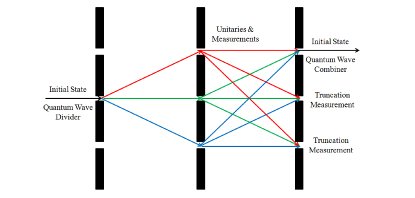
Figure 2: The conceptual physical picture of a 3-slits SWP-DQC. In the middle, the subwaves are manipulated and some auxiliary qubits are projected on to $\ket{0}$ states.

V Some Mathematical Results of SWP-DQC

Here we focus on two mathematical results of SWP-DQC: the success probability and the mean time complexity. We show that SWP-DQC can give a polynomial acceleration compared to DQC with only a final projection.

V.1 Success Probability

Our first mathematical result can be derived by calculating the success probability of the entire algorithm from Eq. (12), Eq. (17) and Eq. (20),

$$P = p_{0}\times p_{1}\times\dots\times p_{M-1}\times p_{M}$$ (21)

$$= \big{(}b_{0}|V_{00}|^{2}+|V_{10}|^{2}+\dots+|V_{M-1,0}|^{2}\big{)}$$

$$\times \frac{b_{0}|V_{00}|^{2}+b_{1}|V_{10}|^{2}+\dots+|V_{M-1,0}|^{2}}{v_{0}|V_{00}|^{2}+|V_{10}|^{2}+\dots+|V_{M-1,0}|^{2}}\times\dots$$

$$\times \frac{b_{0}|V_{00}|^{2}+\dots+b_{M-2}|V_{M-2,0}|^{2}+b_{M-1}|V_{M-1,0}|^{2}}{b_{0}|V_{00}|^{2}+\dots+b_{M-2}|V_{M-2,0}|^{2}+|V_{M-1,0}|^{2}}$$

$$\times \frac{\bra{\Psi}A^{\dagger}A\ket{\Psi}}{b_{0}|V_{00}|^{2}+\dots+b_{M-1}|V_{M-1,0}|^{2}}$$

$$= \bra{\Psi}A^{\dagger}A\ket{\Psi}.$$

The expression of the probability is natural because it is just the norm of the vector $A\ket{\Psi}$, and is less than $1$ because we have assumed that $A$ is a contraction. In DQC with final-wave-projection, the target state is also $\sum_{i=0}^{M-1}c_{i}B_{i}\ket{\Psi}=A\ket{\Psi}$. Therefore, as a probabilistic algorithm, its success probability must also be the square of modulus,

$$P^{\prime}=\bra{\Psi}A^{\dagger}A\ket{\Psi}.$$ (22)

V.2 Mean Time Complexity and SWP-DQC Acceleration

In order to analyze the mean time complexity, we make the following analysis on a model in probability theory. Suppose an event occurs with probability of $p$ in an experiment. It will be terminated once the experiment is successful. If it fails, then we make another experiment. We stop until we succeed to get the event. The probability of success after $s$-time is defined as $P(s)=p(1-p)^{s-1}$. The mean number of experiments will be

$$E=\sum_{s=1}^{\infty}s\cdot p(1-p)^{s-1}=\lim_{i\to\infty}\frac{1-(1-p)^{s}(1+s\cdot p)}{p}=\frac{1}{p}.$$ (23)

The expected value of run time of SWP-DQC can be expressed by the known physical quantity from this model in probability theory. In SWP-DQC, there are several projections on the subwaves, each projection succeeds with a probability $p_{i}$. Because the call of the $i$-th step in the algorithm is equivalent to an event with success probability of $p_{i}p_{i+1}\dots p_{M}$ in a series of experiments. Therefore, the overall mean time of SWP-DQC is the sum of mean time of all steps:

$$Et = \frac{t_{0}}{p_{0}p_{1}\dots p_{M}}+\frac{t_{1}}{p_{1}\dots p_{M}}+\dots+\frac{t_{M-1}}{p_{M-1}p_{M}}$$

$$= \frac{t_{0}+p_{0}t_{1}+(p_{0}p_{1})t_{2}+\dots+(p_{0}p_{1}\dots p_{M-2})t_{M-1}}{p_{0}p_{1}\dots p_{M-1}p_{M}}.$$

Notice that the expectation depends on the order of gates. The optimal order requires complicated numerical calculation.

However, the total time of DQC with final-wave-projection is obviously $t_{0}+t_{1}+t_{2}+\dots+t_{M-1}$, with the success probability of $P^{\prime}=\bra{\Psi}A^{\dagger}A\ket{\Psi}$. Thus, the expected value of run time in DQC with final-wave-projection can be derived of our model in probability theory:

$$Et^{\prime} = \frac{t_{0}+t_{1}+t_{2}+\dots+t_{M-1}}{\bra{\Psi}A^{\dagger}A\ket{\Psi}}=\frac{t_{0}+t_{1}+t_{2}+\dots+t_{M-1}}{p_{0}p_{1}\dots p_{M-1}p_{M}}$$

$$> \frac{t_{0}+p_{0}t_{1}+(p_{0}p_{1})t_{2}+\dots+(p_{0}p_{1}\dots p_{M-2})t_{M-1}}{p_{0}p_{1}\dots p_{M-1}p_{M}}=Et.$$

Even though the numerical calculation in Eq. (V.2) is very troublesome, we can still compare the complexity between $Et$ and $Et^{\prime}$ with some simplified assumptions. Assume that each basic gate has the same time complexity $t_{0}=t_{1}=\dots=t_{M-1}=1$, and the same order of success probability of $p$ (recall the Eq. (17), in each step $p_{i}$ is very close to 1 if $M$ is large enough). Then we can derive that $Et^{\prime}=O(\frac{M}{p^{M}})$, whereas

$$Et=\frac{1+p+\dots+p^{M-1}}{p^{M+1}}=\frac{1-p^{M}}{p^{M}p(1-p)}=O\left(\frac{1}{p^{M}}\right).$$ (26)

Our analysis on the acceleration is only valid in sequential realization of SWP-DQC. It is interesting to study the parallel realization of SWP-DQC, and study its acceleration.

Another point is that, in most cases, $M$ increases rapidly as precision of calculation gets higher. For example, in order to get a higher precision, the larger the evolution time $t$ in a quantum algorithm, the more steps we need to use, which means that $p$ may still be the same, but the complexity of the algorithm increases with the matrix number $M$. In this respect, we say, SWP-DQC has an $O(M)$ speedup compared with DQC with final-wave-projection in time complexity.

VI Application: An optimization of ground state preparation quantum algorithm

Yimin Ge, Jordi Tura, and J. Ignacio Cirac recently proposed a general-purpose quantum algorithm for preparing ground states of a quantum Hamiltonian from a given trial state (we will use GTC algorithm hereafter). Here we show that the GTC algorithm is a DQC algorithm, and we also give an optimization of GTC algorithm by using the SWP-DQC. The optimized algorithm uses $2+\log_{2}N$ less qubits, where $N$ is the dimension of the Hermitian matrix.

VI.1 Brief Description of GTC Algorithm

Here is a brief description of GTC algorithm for ground state preparation Ge et al. (2017). For the $N\times N$ Hermitian matrix $\tilde{H}$, assume $n=\log_{2}N$, and the spectrum of $\tilde{H}$ lies in $[0,1]$, with the lowest eigenvalue $\lambda_{0}$. The spectrum is assumed to be non-degenerate. Let $E\in[0,\lambda_{0}]$ be a known real number, then define $\delta_{E}:=\lambda_{0}-E$ and $H:=(1+E)~{}\mathbb{I}_{n}-\tilde{H}$. Namely, $H$’s spectrum lies in $[E,1-\delta_{E}]$. And also assume that all other eigenvalues of $H$ are $\leq 1-\delta_{E}-\Delta$. The core ideal of this algorithm is that the iteration of $H$ is almost a projector onto the ground state, because the power of $1-\delta_{E}$ is far larger than the power of the other eigenvalues. Ge et al showed that by iteratively performing $H$ on the trial state $\ket{\phi}=\phi_{0}\ket{\lambda_{0}}+\ket{\lambda^{\bot}_{0}}$ for $M_{0}$ times, where

$$M_{0}=O(\frac{1}{\Delta}\log\frac{1}{\left|\phi_{0}\right|\epsilon}),$$ (27)

which is an even integer, the norm of the difference between normalized state $H^{M_{0}}\ket{\phi}$ and $\ket{\lambda_{0}}$ will be less than $\epsilon$.

Figure 3: SWP-DQC for optimized GTC Algorithm, where the first column and row of QWD and QWC is $V_{i0}=W_{0i}=\sqrt{\frac{\alpha_{i}}{\alpha}}$ and $L$ is defined in Eq. (30). We only need one qubit in the second group of auxiliary qubit.

The $M_{0}$ power of $H$ can be calculated using a linear combination of $M$ terms of non-unitary operations to a good approximation, where

$$M=O(\sqrt{\frac{1}{\Delta}}\log\frac{1}{\left|\phi_{0}\right|\epsilon}),$$ (28)

namely,

$$H^{M_{0}}=\sum_{i=0}^{M-1}\alpha_{i}\mathcal{T}_{2i}(H)+O(\left|\phi_{0}\right|\epsilon),$$ (29)

where $\mathcal{T}_{2i}(x)$ represents the $2i$-th Chebyshev polynomials of the first kind, $\alpha_{i}$ is defined as $2^{1-2m_{0}}\bigl{(}\frac{1}{2}\bigr{)}^{\delta_{i0}}\binom{2m_{0}}{m_{0}+i}$, $m_{0}$ is $M_{0}/2$, and $\delta_{i0}$ is the Kronecker delta.

The operation $\sum_{i=0}^{M-1}\alpha_{i}\mathcal{T}_{2i}(H)$ is the linear combination of $M$ non-unitary operations $\mathcal{T}_{2i}(H)$, where $M$ is defined in Eq. (28). It can be obtained by using the following matrix $L$ and its powers

$$L=\left(\begin{array}[]{ccc}H&-(\mathbb{I}-H^{2})^{1/2}\\ (\mathbb{I}-H^{2})^{1/2}&H\end{array}\right),$$ (30)

and

$$L^{n}=\left(\begin{array}[]{ccc}\mathcal{T}_{n}(H)&-(\mathbb{I}-H^{2})^{1/2}\mathcal{U}_{n-1}(H)\\ (\mathbb{I}-H^{2})^{1/2}\mathcal{U}_{n-1}(H)&\mathcal{T}_{n}(H)\end{array}\right).$$ (31)

VI.2 Quantum Circuit for Optimization of GTC Algorithm

The matrix $L$ appearing in Eq. (30) was applied by Ge et al to construct a quantum walk in a larger Hilbert space, namely they doubled the entire system and treated $L$ as an operator on the Hilbert space of $\mathbb{C}^{2N}\otimes\mathbb{C}^{2N}$, which has a dimension of $4N^{2}$. This costs too much qubit resource to complete the task, which adds in $1+\log_{2}(4N^{2}/N)=3+\log_{2}N$ more auxiliary qubits. The GTC ground state preparation algorithm developed requires $2\log_{2}N+\log_{2}M+3$ qubits.

Here we give an optimal algorithm which only uses $\log_{2}N+\log_{2}M+1$ qubits, that is, $2+\log_{2}N$ less qubits, by using SWP-DQC. In our optimized algorithm, it is applied in the Hilbert space $\mathbb{C}^{2}\otimes\mathbb{C}^{2N}$, instead of $\mathbb{C}^{2N}\otimes\mathbb{C}^{2N}$.

Besides the $m=\log_{2}M$ auxiliary qubits in the first group of auxiliary qubits and the $n=\log_{2}N$ work qubits, we add another auxiliary qubit ($p=1$, in the second group of auxiliary qubit). The QWD and QWC can be constructed explicitly as,

$$V_{i0}=W_{0i}=\sqrt{\frac{\alpha_{i}}{\alpha}},$$ (32)

where $\alpha=\sum_{i=0}^{M-1}\alpha_{i}$ (here we have already had $\alpha_{i}\geq 0$), such that the QWD map $\ket{0}^{\otimes m}\ket{0}\ket{\phi}$ to $\sum_{i=0}^{M-1}\sqrt{\frac{\alpha_{i}}{\alpha}}\ket{i}\ket{0}\ket{\phi}$.

For the second group of auxiliary qubit and the work qubits, the quantum state $\ket{0}\ket{\phi}$ in the Hilbert space of $\mathbb{C}^{2}\otimes\mathbb{C}^{N}$ can be written in a matrix form,

$$\ket{0}\otimes\ket{\phi}=\left(\begin{array}[]{c}1\\ 0\end{array}\right)\otimes\bm{\phi}=\left(\begin{array}[]{c}\bm{\phi}\\ 0\end{array}\right).$$ (33)

Notice that $\phi$ is a state, whereas $\bm{\phi}$ is a complex vector.

Then the $2N\times 2N$ unitary matrix $L^{2i}$ in Eq. (30) maps $\ket{0}\otimes\ket{\phi}$ to

$$\left(\begin{array}[]{cc}\mathcal{T}_{n}(H)&-(\mathbb{I}-H^{2})^{1/2}\mathcal{U}_{n-1}(H)\\ (\mathbb{I}-H^{2})^{1/2}\mathcal{U}_{n-1}(H)&\mathcal{T}_{n}(H)\end{array}\right)\left(\begin{array}[]{c}\bm{\phi}\\ 0\end{array}\right)$$ (38)

$$= \left(\begin{array}[]{c}\mathcal{T}_{n}(H)\bm{\phi}\\ (\mathbb{I}-H^{2})^{1/2}\mathcal{U}_{n-1}(H)\bm{\phi}\end{array}\right).$$ (41)

The trial state of work qubits, together with the state of the $M+1$ auxiliary qubits, have been transformed to $M$ subwaves $\sum_{i=0}^{M-1}\sqrt{\frac{\alpha_{i}}{\alpha}}\ket{i}\ket{0}\ket{\phi}$ by QWD. Repeatedly apply the $2MN\times 2MN$ controlled-$L^{2i}$ operation $G_{i}:=\ket{i}\bra{i}\otimes(L^{2i}-\mathbb{I}_{1+n})+\mathbb{I}_{m+1+n}$ ($i=0,1,...,M-1$) and the projection measurements $\mathbb{I}_{m}\otimes\ket{0}\bra{0}\otimes\mathbb{I}_{n}$ for $M$ times, then the quantum system state becomes

$$\sum_{i=0}^{M-1}\sqrt{\frac{\alpha_{i}}{\alpha}}\ket{i}\ket{0}\mathcal{T}_{2i}(H)\ket{\phi}.$$ (42)

Finally, perform the QWC, we get the state

$$\sum_{i=0}^{M-1}\sum_{j=0}^{{M-1}}W_{ji}\sqrt{\frac{\alpha_{i}}{\alpha}}\ket{j}\ket{0}\mathcal{T}_{2i}(H)\ket{\phi}.$$ (43)

Use the projection measurement $\ket{0^{m}}\bra{0^{m}}\otimes\mathbb{I}\otimes\mathbb{I}_{n}$ again. If the output is $\ket{0}^{\otimes p}$, then the final state of the entire quantum system will collapse to $\sum_{i=0}^{M-1}W_{0i}\sqrt{\frac{\alpha_{i}}{\alpha}}\ket{0}^{\otimes m}\ket{0}\mathcal{T}_{2i}(H)\ket{\phi}=\sum_{i=0}^{M-1}\frac{\alpha_{i}}{\alpha}\ket{0}^{\otimes m}\ket{0}\mathcal{T}_{2i}(H)\ket{\phi}$. The quantum circuit of this SWP-DQC optimized algorithm is shown in Figure VI.1.

Note that as the precision becomes higher, GTC algorithm requires more number of Chebyshev polynomials $M$, and the mean time required by GTC algorithm becomes larger. The mean time required by our optimized algorithm requires only $O(1/M)$ of that of the GTC algorithm, as discussed in IV.

VII Summary

In this article, we presented a DQC with subwave projections, the SWP-DQC. Explicit quantum circuit of SWP-DQC is constructed. We proved that the mean time complexity has an $O(M)$ acceleration compared to DQC with only final-wave-projection. We also find the run time depends on the orders of the controlled gates, and this is especially important in the future in constructing programs for concrete problems.

As an application, we show that the ground state preparation proposed by Ge, Tura, and Cirac is a DQC algorithm. We constructed an optimization of GTC algorithm, and it not only saves $(2+\log_{2}N)$ qubits, but also provides additional acceleration in the expected time. It is also found that the order of the gate sets $\left\{L^{2i}\right\}$ is important to obtain the shortest mean run time of the SWP-DQC algorithm.

Acknowledgement

This work was supported by the National Basic Research Program of China under Grant Nos. 2017YFA0303700 and  2015CB921001, National Natural Science Foundation of China under Grant Nos. 61726801,  11474168 and  11474181, and in part by the Beijing Advanced Innovation Center for Future Chip (ICFC).

References

- Long (2005) G. L. Long, arXiv preprint quant-ph/0512120 (2005).
- Gui-Lu (2006) L. Gui-Lu, Communications in Theoretical Physics 45, 825 (2006).
- Gui-Lu and Yang (2008) L. Gui-Lu and L. Yang, Communications in Theoretical Physics 50, 1303 (2008).
- Gui-Lu et al. (2009) L. Gui-Lu, L. Yang, and W. Chuan, Communications in Theoretical Physics 51, 65 (2009).
- Gudder (2007) S. Gudder, Quantum Information Processing 6, 37 (2007).
- Long (2008) G. L. Long, Quantum Information Processing 7, 137 (2008).
- Long (2011) G. L. Long, International Journal of Theoretical Physics 50, 1305 (2011).
- Cao et al. (2010) H. Cao, L. Li, Z. Chen, Y. Zhang, and Z. Guo, Chinese Science Bulletin 55, 2122 (2010).
- Cao et al. (2013) H.-X. Cao, G.-L. Long, Z.-H. Guo, and Z.-L. Chen, International Journal of Theoretical Physics 52, 1751 (2013).
- Zhang et al. (2010) Y. Zhang, H. Cao, and L. Li, Science China Physics, Mechanics and Astronomy 53, 1878 (2010).
- Chen et al. (2015) L. Chen, H.-X. Cao, and H.-X. Meng, Quantum Information Processing 14, 4351 (2015).
- Chen and Cao (2009) Z.-L. Chen and H.-X. Cao, International Journal of Theoretical Physics 48, 1669 (2009).
- Zou et al. (2009) X. Zou, D. Qiu, L. Wu, L. Li, and L. Li, Quantum Information Processing 8, 37 (2009).
- Wu et al. (2014) Z. Wu, S. Zhang, and C. Zhu, Hacettepe J Math Stat 43, 451 (2014).
- Childs and Wiebe (2012) A. M. Childs and N. Wiebe, arXiv preprint arXiv:1202.5822 (2012).
- Shor (1994) P. W. Shor, in Foundations of Computer Science, 1994 Proceedings., 35th Annual Symposium on (Ieee, 1994) pp. 124–134.
- Grover (1996) L. K. Grover, in Proceedings of the twenty-eighth annual ACM symposium on Theory of computing (ACM, 1996) pp. 212–219.
- Long (2001) G.-L. Long, Physical Review A 64, 022307 (2001).
- Wan-Ying et al. (2007) W. Wan-Ying, S. Bin, W. Chuan, and L. Gui-Lu, Communications in Theoretical Physics 47, 471 (2007).
- Harrow et al. (2009) A. W. Harrow, A. Hassidim, and S. Lloyd, Physical Review Letters 103, 150502 (2009).
- Hao et al. (2010) L. Hao, D. Liu, and G. Long, Science China Physics, Mechanics and Astronomy 53, 1765 (2010).
- Berry et al. (2015) D. W. Berry, A. M. Childs, R. Cleve, R. Kothari, and R. D. Somma, Physical review letters 114, 090502 (2015).
- Wei and Long (2016) S.-J. Wei and G.-L. Long, Quantum Information Processing 15, 1189 (2016).
- Wei et al. (2016) S.-J. Wei, D. Ruan, and G.-L. Long, Scientific Reports 6, 30727 (2016).
- Wei et al. (2017) S.-J. Wei, Z.-R. Zhou, D. Ruan, and G.-L. Long, Vehicular Technology Conference (VTC Spring), 2017 IEEE 85th , 1 (2017).
- Qiang et al. (2017) X. Qiang, X. Zhou, K. Aungskunsiri, H. Cable, and J. L. O’Brien, Quantum Science and Technology 2, 045002 (2017).
- Qiang et al. (2018) X. Qiang, X. Zhou, J. Wang, C. M. Wilkes, T. Loke, S. O’Gara, L. Kling, G. D. Marshall, R. Santagati, T. C. Ralph, et al., Nature Photonics 12, 534 (2018).
- Marshman et al. (2018) R. J. Marshman, A. P. Lund, P. P. Rohde, and T. C. Ralph, Physical Review A 97, 022324 (2018).
- Wei et al. (2018) S.-J. Wei, T. Xin, and G.-L. Long, SCIENCE CHINA Physics, Mechanics & Astronomy 61, 070311 (2018).
- Long et al. (2018) G. Long, W. Qin, Z. Yang, and J.-L. Li, Science China Physics, Mechanics & Astronomy 61, 030311 (2018).
- Roy et al. (2012) S. S. Roy, A. Shukla, and T. Mahesh, Physical Review A 85, 022109 (2012).
- Xin et al. (2015) T. Xin, H. Li, B.-X. Wang, and G.-L. Long, Physical Review A 92, 022126 (2015).
- Zhou et al. (2017) Z.-Y. Zhou, Z.-H. Zhu, S.-L. Liu, Y.-H. Li, S. Shi, D.-S. Ding, L.-X. Chen, W. Gao, G.-C. Guo, and B.-S. Shi, Science Bulletin 62, 1185 (2017).
- Qin et al. (2018) W. Qin, A. Miranowicz, G. Long, J. You, and F. Nori, arXiv preprint arXiv:1807.03194 (2018).
- Zhu (2018) Z.-H. Zhu, Science China Physics, Mechanics & Astronomy 61, 050331 (2018).
- Zheng et al. (2013) C. Zheng, J.-L. Li, S.-Y. Song, and G. L. Long, JOSA B 30, 1688 (2013).
- Zheng and Wei (2018) C. Zheng and S. Wei, International Journal of Theoretical Physics , 1 (2018).
- Zheng (2018) C. Zheng, EPL (Europhysics Letters) 123, 40002 (2018).
- Huang et al. (2018) L. Huang, X. Wu, and T. Zhou, Science China Physics, Mechanics & Astronomy 61, 080311 (2018).
- Liu and Cui (2014) Y. Liu and J.-X. Cui, Chinese Science Bulletin 59, 2298 (2014).
- Cui et al. (2012) J. Cui, T. Zhou, and G. L. Long, Quantum Information Processing 11, 317 (2012).
- Nielsen and Chuang (2002) M. A. Nielsen and I. Chuang, “Quantum computation and quantum information,” (2002).
- Ge et al. (2017) Y. Ge, J. Tura, and J. I. Cirac, arXiv preprint arXiv:1712.03193 (2017).
- Wu (1994) P. Wu, Banach Center Publications 30, 337 (1994).
- Wang et al. (2008) Y.-Q. Wang, H.-K. Du, and Y.-N. Dou, International Journal of Theoretical Physics 47, 2268 (2008).