Compressive Privacy for a
Linear Dynamical System

Abstract

We consider a linear dynamical system in which the state vector consists of both public and private states. One or more sensors make measurements of the state vector and sends information to a fusion center, which performs the final state estimation. To achieve an optimal tradeoff between the utility of estimating the public states and protection of the private states, the measurements at each time step are linearly compressed into a lower dimensional space. Under the centralized setting where all measurements are collected by a single sensor, we propose an optimization problem and an algorithm to find the best compression matrix. Under the decentralized setting where measurements are made separately at multiple sensors, each sensor optimizes its own local compression matrix. We propose methods to separate the overall optimization problem into multiple sub-problems that can be solved locally at each sensor. We consider the cases where there is no message exchange between the sensors; and where each sensor takes turns to transmit messages to the other sensors. Simulations and empirical experiments demonstrate the efficiency of our proposed approach in allowing the fusion center to estimate the public states with good accuracy while preventing it from estimating the private states accurately.

I Introduction

In the emerging Internet of Things (IoT) paradigm, large numbers of sensors are deployed in modern infrastructures, such as smart grids, population health monitoring, traffic monitoring, online recommendation systems, etc. [1, 2, 3, 4, 5, 6]. These sensors make observations and send data like the level of power consumption, sickness symptoms, or GPS coordinates in real-time to a fusion center [7, 8, 9, 10, 11], thus allowing utility companies and other service providers to improve their service offerings. However, some privacy-sensitive information such as personal activities, behaviors, preferences, habits and health conditions can be inferred from the raw measurements collected from individuals. For example, in a smart grid infrastructure, customers could be offered better rates if they continuously send their instantaneous power consumption to the utility company, which helps to improve the demand forecasting mechanism. However, from the fine-grained smart meter readings, the customers’ private activities such as when and for how long appliances are used can be inferred [12, 13, 14]. Another example is the inference of individuals’ private ratings or preferences from temporal changes in public recommendation systems [15, 16]. In traffic monitoring systems, individual users send anonymized personal location traces, which can be GPS coordinates measured by their smartphones, to a data aggregator to aid in traffic state estimation. However, an adversary may link an anonymous GPS trace to a particular person provided the knowledge of the person’s residence and/or working location [17, 18, 19, 20]. Therefore, it is essential to develop privacy preserving mechanisms to protect private state information from being inferred while retaining the quality of services that depend on the sensor measurements. All the above mentioned applications involve dynamic and time-varying data streams instead of static data sets.

In this paper, we consider a linear dynamical system (LDS) in which one or more sensors make measurements of the evolving state vector, and send information to a fusion center that makes the final state estimation. Suppose some of the states contain sensitive information. We call these states the private states, while the remaining states are public states. Our goal is to allow the fusion center to estimate the public states while making it difficult for it to estimate the private states. To achieve this, each sensor sanitizes its measurement to remove statistical information about the private states before sending it to the fusion center. A naive approach is for each sensor to first estimate the public states and send only this information to the fusion center. Such an approach does not prevent statistical inference of the private states at a future time step since in a LDS, the public states at one time step may provide statistical information about the private states in a future time step. Furthermore, when there are more than one sensor, it may not be possible for each individual sensor to estimate the public states. There is therefore a need to investigate the optimal way to sanitize information to achieve the best tradeoff between the utility of estimating the public states and the protection of the private states over all time steps. In this paper, we consider the use of a linear transformation or compression to map the sensor measurements into a lower dimensional space as the sanitization procedure. We call this compressive privacy [21].

I-A Related Work

In general, privacy can be categorized into two classes: data privacy and inference privacy [22, 23, 24, 25]. Data privacy protects the original measurements from being inferred by fusion center. The privacy metrics that have been proposed for preserving data privacy in a sensor network include homomorphic encryption [26, 27, 28], $k$-anonymity [29], plausible deniability [30] and local differential privacy [31, 32, 33, 34, 35]. Inference privacy on the other hand, prevents the fusion center from making certain statistical inferences. The privacy metrics that have been proposed to achieve inference privacy include information privacy [36, 37, 23, 25], differential privacy [38, 39, 40], Blowfish privacy [41], mutual information privacy [42, 43] and average information leakage [44, 45]. The relationship between data privacy and inference privacy has been studied in [42, 24].

The type of privacy we consider in this paper can be considered to be a form of inference privacy since we wish to prevent the fusion center from inferring about the private states. The aforementioned inference privacy metrics like information privacy, differential privacy, mutual information privacy and average information leakage either assume a finite state alphabet (and are thus more applicable in a hypothesis testing context instead of an estimation context), or do not directly guarantee that the fusion center cannot estimate the private states to within a certain error, making the choice of the privacy budgets in these metrics unclear and unintuitive. Furthermore, although quantities like mutual information have relationships with estimation error, they are not as easy to work with in a LDS where we consider privacy over multiple time steps. Therefore, in this paper, we define privacy on the estimation error variance instead, and require that the estimation error variances of the private states to be above a predefined threshold.

The papers [46, 47, 48, 49] proposed to extract the relevant aspects of the data by the information bottleneck (IB) approach. Given the joint distribution of a “source" variable $\mathbf{z}$ and another “relevance" variable ${\bf y}$, IB compresses $\mathbf{z}$ to obtain $\tilde{\mathbf{z}}=\mathbf{C}\mathbf{z}$, while preserving information about ${\bf y}$. IB tradeoffs the complexity of the representation of $\mathbf{z}$, measured by the mutual information $I(\mathbf{z};\tilde{\mathbf{z}})$ , against the accuracy of this representation measured by $I(\mathbf{y};\tilde{\mathbf{z}})$. The compression is designed to make $I(\mathbf{z};\tilde{\mathbf{z}})$ small and $I(\mathbf{y};\tilde{\mathbf{z}})$ large. We can interpret $\mathbf{y}$ to be the public state or information while $\mathbf{z}$ to be the private state. The privacy funnel (PF) method [50] uses a mapping from the source variable $\mathbf{z}$ to $\tilde{\mathbf{z}}=\mathbf{C}\mathbf{z}$ so that $I(\mathbf{y};\tilde{\mathbf{z}})$ is small and $I(\mathbf{z};\tilde{\mathbf{z}})$ is large. PF operates in a way that is opposite to IB by treating $\mathbf{y}$ as the private state. Both IB and PF do not consider information over multiple time steps, and are not directly applicable to a LDS without additional prior information about the LDS evolution.

The papers [51, 21, 52, 53, 54, 55, 56] introduced the concept of compressive privacy (CP), which is a dimension-reducing subspace approach. They considered the case where the source variable $\mathbf{z}$ can be mapped as $\bm{\Gamma}^{(\mathcal{P})}\mathbf{z}$ to the utility subspace and as $\bm{\Gamma}^{(\mathcal{Q})}\mathbf{z}$ to the privacy subspace, where $\bm{\Gamma}^{(\mathcal{P})}$ and $\bm{\Gamma}^{(\mathcal{Q})}$ are projection matrices. Under the assumption that $\mathbf{z}$ has a Gaussian distribution, the compression matrix $\mathbf{C}$ is designed to achieve an optimal privacy-utility tradeoff based on $I(\bm{\Gamma}^{(\mathcal{P})}\mathbf{z};\tilde{\mathbf{z}})$ and $I(\bm{\Gamma}^{(\mathcal{Q})}\mathbf{z};\tilde{\mathbf{z}})$, where $\tilde{\mathbf{z}}=\mathbf{C}\mathbf{z}$. In the case where the projection matrices $\bm{\Gamma}^{(\mathcal{P})}$ and $\bm{\Gamma}^{(\mathcal{Q})}$ are unknown, a machine learning approach is proposed to learn the compression matrix $\mathbf{C}$ from a set of training data. Our formulation is similar to [21], except that we assume that the underlying state vector generating the measurement $\mathbf{z}$ can be divided into public and private states, instead of the measurement $\mathbf{z}$ being mapped into utility and privacy subspaces. A more detailed technical discussion of the differences is provided in Section II. Furthermore, different from [51, 21, 52, 53] which considers $\mathbf{z}$ to be a single-shot observation, we consider a LDS in which observations are temporally correlated, and our goal is to preserve the privacy of the private states over multiple future time steps.

The references [57, 58] developed differential privacy mechanisms for the measurements $\mathbf{z}_{k}$, $k=1,2,\ldots$, in a LDS. The authors of [57] proposed to use an input perturbation mechanism so that $\tilde{\mathbf{z}}_{k}=\mathbf{z}_{k}+\bm{\nu}_{k}$, where $\bm{\nu}_{k}$ is white Gaussian noise, is used in place of $\mathbf{z}_{k}$ at each time step $k$ to guarantee $(\epsilon,\delta)$-differential privacy for the original measurement $\mathbf{z}_{k}$. The paper [58] proposed to apply an input perturbation mechanism together with a linear transformation, i.e., $\tilde{\mathbf{z}}_{k}=\mathbf{C}\mathbf{z}_{k}+\bm{\nu}_{k}$. By adding white Gaussian noise $\bm{\nu}_{k}$ according to the Gaussian mechanism [59], $\mathbf{C}\mathbf{z}_{k}$ is differentially private. The transformation matrix $\mathbf{C}$ is designed to minimize the mean-square error (MSE) of the states. These papers’ objectives are to preserve the differential privacy of the system measurements, which is different from our goal of preventing the statistical inference of a subset of states.

The authors in [60] proposed to project an observation $\mathbf{z}$ into a lower dimensional space to obtain $\tilde{\mathbf{z}}=\mathbf{C}\mathbf{z}$. The transformation $\mathbf{C}$ is designed to maximally retain the estimation accuracy of the entire system’s state and the dimension of the space projected into is predefined. This work also does not consider preserving the estimation privacy of a subset of states in a LDS.

I-B Our Contributions

In this paper, we consider the use of a compressive linear transformation on the measurements at one or multiple sensors in a LDS to prevent the fusion center from estimating a set of private states with low error while still allowing it to estimate a set of public states with good accuracy. Our main contributions are as follows.

1. We formulate a utility-privacy tradeoff optimization problem for a LDS involving privacy constraints on the predicted estimation error of the private states multiple steps ahead. We show how to find the dimension of the compressive map and the map itself and propose an algorithm to achieve this. We provide a bound for the number of steps to look ahead to achieve the same privacy level in all future time steps.

2. We consider the case where there are multiple decentralized sensors that optimize their own local compressive map. We propose optimization methods for the cases where 1) there are no message exchanges between the sensors; and 2) each sensor takes turns to transmit messages to the other sensors.

3. We present extensive simulation results that demonstrate that imposing privacy constraints multiple steps ahead is necessary in some LDSs, and examine the impact of different choices of the state evolution and measurement matrices on the utility-privacy tradeoff. We also verify the performance of our proposed approach on an empirical ultra wideband (UWB) localization system and human activity recognition data set.

TABLE I: Summary of commonly-used symbols.

Notation	Definition
$\mathcal{P}=\{1,\ldots,|\mathcal{P}|\}$	index set of the $|\mathcal{P}|$ public states
$\mathcal{Q}=\{|\mathcal{P}|+1,\ldots,L\}$	index set of the $|\mathcal{Q}|=L-|\mathcal{P}|$ private states
$\mathbf{x}_{k}$, $\mathbf{z}_{k}$	state and measurement vector at time $k$, respectively
$\mathbf{F}_{k}\in\mathbb{R}^{L\times L}$, $\mathbf{H}_{k}\in\mathbb{R}^{N\times L}$	state evolution and measurement matrices at time $k$, 1
$\mathbf{Q}_{k}$, $\mathbf{R}_{k}$	state and measurement noise covariances at time $k$, 1
$\mathbf{C}_{k}\in\mathbb{R}^{M\times N}$	compression matrix applied to the measurement at time $k$, 7
$\tilde{\mathbf{P}}_{k+n|k}$	$n$-step prediction error covariance matrix after compression at time $k$, 13
$\mathbf{T}_{k}$	$={\bf H}_{k}\tilde{\mathbf{P}}_{k|k-1}{\bf H}^{\intercal}_{k}+{\bf R}_{k}$, 15
${\bf G}_{k+n|k}$	$={\bf H}_{k}\tilde{\mathbf{P}}_{k|k-1}\mathbf{F}_{k+1:k+n}^{\intercal}$, 16
$\mathbf{D}_{k+n|k}$	$\tilde{\mathbf{P}}_{k+n|k}-\tilde{\mathbf{P}}_{k+n|k-1}$, error reduction due to measurement made at time $k$, 19
$\tau_{k}(\mathbf{C}_{k})$	public error trace at time $k$ , 8
$\eta_{k+n|k}(\mathbf{C}_{k})$	$n$-step look-ahead private error function at time $k$ with $\eta_{k}=\eta_{k|k}$, 14
$u_{k}(\mathbf{C}_{k})$	utility at time $k$, 22
$\ell_{k+n|k}(\mathbf{C}_{k})$	$n$-step look ahead privacy loss at time $k$, 23

A preliminary version of this work was presented in [61] in which only the single sensor case with a single step look-ahead privacy constraint was considered. This paper generalizes [61] to the case where there are multiple decentralized sensors with multi-step look-ahead privacy constraints. New theoretical insights and numerical results are also presented in this paper.

The rest of this paper is organized as follows. In Section II, we present our problem formulation, assumptions and an optimization framework to achieve an optimal utility-privacy tradeoff. In Section III, we propose a centralized solution to find the compression matrix that optimizes the utility-privacy tradeoff at each time step. In Section IV, we consider the decentralized case where multiple sensors are involved and proposed different optimization approaches. We present simulation results in Section V, and conclude in Section VII.

Notations: We use $\mathbb{R}$ to denote the set of real numbers. The normal distribution with mean $\mu$ and variance $\sigma^{2}$ is denoted as ${\cal N}(0,\sigma^{2})$. $\min(\mathbf{a})$ is the minimum element in the vector $\mathbf{a}$, $\bm{1}_{n}$ is the vector of all 1’s of length $n$, and $\mathbf{I}_{n}$ is the identity matrix of size $n\times n$. We use ^⊺ to represent matrix transpose, ${\rm diag}({\bf A},{\bf B},\ldots)$ to represent a block diagonal matrix with submatrices ${\bf A},{\bf B},\ldots$ being the diagonal elements, ${\rm Tr}(\cdot)$ to denote the trace operation, and ${\rm vecdiag}(\mathbf{A})$ to denote a column vector consisting of diagonal entries of $\mathbf{A}$. We use $\left[\mathbf{A}\right]_{\mathcal{P},\mathcal{Q}}$ to denote the sub-matrix of matrix ${\bf A}$ consisting of the entries ${\bf A}(i,j)$ for all $(i,j)\in\mathcal{P}\times\mathcal{Q}$, $\left[{\bf A}\right]_{:,\mathcal{Q}}$ to denote the sub-matrix of matrix ${\bf A}$ consisting of columns indexed by $\mathcal{Q}$, and $\left[{\bf A}\right]_{\mathcal{P}}$ to denote the sub-matrix of matrix ${\bf A}$ consisting of rows indexed by $\mathcal{P}$. Given a set of $n\times n$ matrices ${\bf A}_{i},{\bf A}_{i+1},\ldots,{\bf A}_{j}$, we use $\mathbf{A}_{i:j}$ to denote the matrix product $\mathbf{A}_{j}\mathbf{A}_{j-1}\cdots\mathbf{A}_{i}$ if $i\leq j$, and define $\mathbf{A}_{i:j}=\mathbf{I}_{n}$ if $i>j$. The notation ${\bf A}\succeq{\bf 0}$ means that ${\bf A}$ is positive semidefinite. Let $\mathbf{A}^{\perp}$ denote the basis matrix of the null space of $\mathbf{A}$, i.e., $\mathbf{A}^{\intercal}\mathbf{A}^{\perp}={\bf 0}$. For easier reference, we summarize some of the commonly-used symbols in Table I.

II Problem Formulation

We consider a LDS given by the following state and measurement equations at time step $k$:

$${\bf x}_{k} ={\bf F}_{k}{\bf x}_{k-1}+{\bf v}_{k},$$ (1a)

$$\mathbf{z}_{k} ={\bf H}_{k}{\bf x}_{k}+{\bf n}_{k},$$ (1b)

where ${\bf x}_{k}\in\mathbb{R}^{L}$ and $\mathbf{z}_{k}\in\mathbb{R}^{N}$ are the system’s state and measurement at time $k$, respectively. The state and process noise ${\bf v}_{k}$ and ${\bf n}_{k}$ are independent, and follow zero-mean Gaussian distributions with positive definite covariances ${\bf Q}_{k}$ and ${\bf R}_{k}$, respectively. We assume that the state evolution matrices ${\bf F}_{k}\in\mathbb{R}^{L\times L}$ are known for all $k$, and the measurement matrices $\{{\bf H}_{j}\in\mathbb{R}^{N\times L}:j\leq k\}$, where $N\geq L$ are known only up to the current time step $k$. This assumption is made because in many applications like target tracking [62, 63, 64], the measurement matrix $\mathbf{H}_{k}$ is chosen adaptively at each time step $k$.

Another example is estimation over lossy networks where the measurement matrices are time-varying [65, 66]. On their routes to the gateway, sensor packets, possibly aggregated with measurements from several nodes, may become intermittent because of time-varying transmission intervals or delays [67, 68], packet dropouts [69, 70, 71, 72, 73, 74, 75, 76, 68], random message exchanges depending on the availability of appropriate network links [77], fading channels [78], and other communication constraints [79]. The measurement matrix $\mathbf{H}_{k}$ is thus unknown until the sensor measurements are received at time $k$.

To obtain the minimum mean square estimate of the system state in 1, it is well known [80] that the Kalman filter is optimal. The Kalman filter contains two distinct phases: “predict" and “update". In the “predict" phase, the state estimate and error covariance are predicted, respectively, by

$$\hat{\bf x}_{k|k-1} ={\bf F}_{k}\hat{\bf x}_{k-1|k-1},$$ (2)

$$\mathbf{P}_{k|k-1} ={\bf F}_{k}\mathbf{P}_{k-1|k-1}{\bf F}^{\intercal}_{k}+{\bf Q}_{k}.$$ (3)

In the “update" phase, the state estimate and error covariance are updated, respectively, through

$$\hat{\bf x}_{k|k} =\hat{\bf x}_{k-1|k-1}+{\bf K}_{k}(\mathbf{z}_{k}-{\bf H}_{k}\hat{\bf x}_{k|k-1}),$$ (4)

$$\mathbf{P}_{k|k} =({\bf I}-{\bf K}_{k}{\bf H}_{k})\mathbf{P}_{k|k-1},$$ (5)

where ${\bf K}_{k}=\mathbf{P}_{k|k-1}{\bf H}_{k}^{\intercal}\left({\bf H}_{k}\mathbf{P}_{k|k-1}{\bf H}^{\intercal}_{k}+{\bf R}_{k}\right)^{-1}$ denotes the Kalman gain.

In this paper, we consider the case where the state ${\bf x}_{k}$ may be partitioned into two parts as

$$\mathbf{x}_{k} =\begin{bmatrix}\left[\mathbf{x}_{k}\right]_{\mathcal{P}}\\ \left[\mathbf{x}_{k}\right]_{\mathcal{Q}}\end{bmatrix},$$ (6)

where $\left[{\bf x}_{k}\right]_{\mathcal{P}}\in\mathbb{R}^{|\mathcal{P}|}$, with $\mathcal{P}=\{1,\ldots,|\mathcal{P}|\}$ and $|\mathcal{P}|<L$, contains the public states that are to be estimated, while $\left[{\bf x}_{k}\right]_{\mathcal{Q}}\in\mathbb{R}^{|\mathcal{Q}|}$, with $\mathcal{Q}=\{|\mathcal{P}|+1,\ldots,L\}$ and $|\mathcal{Q}|=L-|\mathcal{P}|>0$, are the private states containing sensitive information that we wish to protect. Our goal is to minimize the estimation errors of the public states $\left[\hat{\bf x}_{k|k}\right]_{\mathcal{P}}$, while ensuring that the estimation errors of private states $\left[\hat{\bf x}_{k|k}\right]_{\mathcal{Q}}$ are above a predefined threshold.

In [21], it is assumed that the measurement or feature vector $\mathbf{z}_{k}$ can be mapped as $\bm{\Gamma}^{(\mathcal{P})}\mathbf{z}_{k}$ to a utility subspace and as $\bm{\Gamma}^{(\mathcal{Q})}\mathbf{z}_{k}$ to a privacy subspace. Our formulation is equivalent to a variant of the formulation in [21] if there is no additive noise $\mathbf{n}_{k}$ in 1b, and $[\mathbf{H}_{k}]_{:,\mathcal{P}}$ is orthogonal to $[\mathbf{H}_{k}]_{:,\mathcal{Q}}$, but is in general different from [21]. The advantage of our formulation is that in applications with a known LDS model, it is easier to specify which system states are public and private directly instead of through the measurements or observed features. Furthermore, to apply the formulation from [21] to a LDS where we want to protect the privacy of some states over multiple time steps, will require prior knowledge of the measurement matrices $\mathbf{H}_{j}$ for $j\geq k$, where $k$ is the current time step. In particular, such an approach is impractical if $j$ is large.

To prevent the fusion center from inferring the private states $[\mathbf{x}_{k}]_{\mathcal{Q}}$, we assume that a linear mapping or compression matrix $\mathbf{C}_{k}\in\mathbb{R}^{M\times N}$, where $1\leq M\leq N$, is applied to the measurement to obtain

$$\tilde{\mathbf{z}}_{k}=\mathbf{C}_{k}\mathbf{z}_{k} =\mathbf{C}_{k}{\bf H}_{k}{\bf x}_{k}+\mathbf{C}_{k}{\bf n}_{k}.$$ (7)

Let $\tilde{\mathbf{P}}_{k|k}$ be the state error covariance based on the measurements $\tilde{\mathbf{z}}_{k^{\prime}}$, where $k^{\prime}\leq k$.

A smaller $\tilde{\mathbf{P}}_{k|k}(i,i)$ implies that the $i$-th state can be estimated with lower error on average. Therefore, as the utility, we aim to minimize the sum of the expected estimation errors of the public states or the public error trace at time $k$ defined as

$$\tau_{k}\left(\mathbf{C}_{k}\right)={\rm Tr}\left(\left[\tilde{\mathbf{P}}_{k|k}\right]_{\cal P,P}\right).$$ (8)

On the other hand, the private error function at time $k$ is defined as

$$\eta_{k}\left(\mathbf{C}_{k}\right)={\cal F}\left({\rm vecdiag}\left(\left[\tilde{\mathbf{P}}_{k|k}\right]_{\cal Q,Q}\right)\right),$$ (9)

where $\mathcal{F}(\mathbf{x})=\mathbf{A}\mathbf{x}:\mathbb{R}^{|\mathcal{Q}|}\rightarrow\mathbb{R}^{|\mathcal{F}|}$ is a user-defined linear map such that $\mathcal{F}(\mathbf{a})\leq\mathcal{F}(\mathbf{b})$ if $\mathbf{a}\leq\mathbf{b}$, with $\leq$ here denoting element-wise inequality. The non-decreasing property follows iff $\mathbf{A}$ has non-negative entries.

For example, if ${\cal F}(\mathbf{x})={\bf 1}^{T}_{|{\cal Q}|}\mathbf{x}$ with $|\mathcal{F}|=1$, the private error function is the sum of the private states’ error variances and

$$\eta_{k}\left(\mathbf{C}_{k}\right)={\rm Tr}\left(\left[\tilde{\mathbf{P}}_{k|k}\right]_{\cal Q,Q}\right).$$ (10)

If the privacy of every private state is important, we can choose ${\cal F}(\mathbf{x})=\mathbf{I}_{\mathcal{Q}}\mathbf{x}$ and $|\mathcal{F}|=|\mathcal{Q}|$. Then, the private error function becomes

$${\bm{\eta}}_{k}\left(\mathbf{C}_{k}\right)={\rm vecdiag}\left(\left[\tilde{\mathbf{P}}_{k|k}\right]_{\cal Q,Q}\right).$$ (11)

At each time $k$, we seek to optimize the privacy-utility tradeoff myopically as follows:

$$\min_{\mathbf{C}_{k}} ~{}\tau_{k}(\mathbf{C}_{k}),$$

$${\rm s.t.} ~{}\eta_{k}(\mathbf{C}_{k})\geq{\cal F}(\delta{\bf 1}_{|{\cal Q}|}),$$

where $\delta$ is a predefined threshold, and the minimization is over the set of compression matrices $\{\mathbf{C}_{k}:\mathbf{C}_{k}\in\mathbb{R}^{M},\ 1\leq M\leq N\}$. Note that we are optimizing over $\mathbf{C}_{k}$ as well as its dimension, i.e., $M$, at every time step and Section II is solved sequentially for each time step $k$.

The private error function given in 11 is more restrictive than that given in 10. In many practical problems, the private information depends on all the private states so that protecting some (but not necessarily all) of the private states may be sufficient to protect the overall private information. For example, to protect someone’s geo-location information, which consists of $x$-, $y$- and $z$- coordinates, it may be sufficient in some applications to obfuscate just one or two coordinates instead of all three to achieve reasonable geo-location privacy. This motivates the use of the private error trace in 10 as one potential privacy measure.

Problem Section II focuses on the privacy-utility tradeoff at the current time step without taking into account the future time steps. As the predicted error covariance $\tilde{\mathbf{P}}_{k+1|k}$ relates to the error covariance $\tilde{\mathbf{P}}_{k|k}$ through 3, i.e.,

$$\tilde{\mathbf{P}}_{k+1|k}={\bf F}_{k+1}\tilde{\mathbf{P}}_{k|k}{\bf F}^{\intercal}_{k+1}+{\bf Q}_{k+1},$$ (12)

$\mathbf{C}_{k}$ affects not just the privacy-utility tradeoff at the current time step $k$, but also the tradeoff at future time steps. This is illustrated in an example below.

Example 1.

Consider the case where $\left[{\bf F}_{k}\right]_{\cal P,P}=0$ and $\left[{\bf F}_{k}\right]_{\cal Q,Q}=0$, i.e.,

$${\bf F}_{k} =\left[\begin{array}[]{cc}{\bf 0}&\left[{\bf F}_{k}\right]_{\cal P,Q}\\ \left[{\bf F}_{k}\right]_{\cal Q,P}&{\bf 0}\end{array}\right].$$

Recall that the prediction error covariance $\mathbf{P}_{k|k-1}$ is related to $\mathbf{P}_{k-1|k-1}$ via 3. Substituting ${\bf F}_{k}$ into 2 and 3 yields

$$\left[\begin{array}[]{c}\left[\hat{\bf x}_{k|k-1}\right]_{\mathcal{P}}\\ \left[\hat{\bf x}_{k|k-1}\right]_{\mathcal{Q}}\end{array}\right] =\left[\begin{array}[]{c}\left[{\bf F}_{k}\right]_{\cal P,Q}\left[\hat{\bf x}_{k-1|k-1}\right]_{\mathcal{Q}}\\ \left[{\bf F}_{k}\right]_{\cal Q,P}\left[\hat{\bf x}_{k-1|k-1}\right]_{\mathcal{P}}\end{array}\right],$$

$$\mathbf{P}_{k|k-1} =\left[\begin{array}[]{cc}\left[{\bf F}_{k}\right]_{\cal P,Q}\left[\mathbf{P}_{k-1|k-1}\right]_{\cal Q,Q}\left[{\bf F}_{k}\right]_{\cal Q,P}&*\\ &\left[{\bf F}_{k}\right]_{\cal Q,P}\left[\mathbf{P}_{k-1|k-1}\right]_{\cal P,P}\left[{\bf F}_{k}\right]_{\cal P,Q}\end{array}\right]+{\bf Q}_{k}.$$

We see that the state evolution matrix ${\bf F}_{k}$ converts the public state at time $k-1$ into a linear function of the private state at time $k$, and vice versa. This means that if a low public error trace is achieved at time $k-1$, then a low private error function value at time $k$ is inevitable if Section II is used to design the utility-privacy tradeoff. This example shows that it is necessary to incorporate privacy constraints for future time steps into Section II.

Since the dynamical model 1a is publicly known, we may predict the system’s state $n$ time steps in the future. The $n$-step prediction error covariance $\tilde{\mathbf{P}}_{k+n|k}$ at time $k$ is given by

$$\tilde{\mathbf{P}}_{k+n|k} =\mathbf{F}_{k+1:k+n}\tilde{\mathbf{P}}_{k|k}{\mathbf{F}^{\intercal}_{k+1:k+n}}+\sum_{i=1}^{n}{\bf F}_{k+i+1:k+n}{\bf Q}_{k+i}{{\bf F}^{\intercal}_{k+i+1:k+n}}.$$ (13)

The look-ahead private error function at time $k+n$ can be defined as

$$\eta_{k+n|k}(\mathbf{C}_{k})={\cal F}\left({\rm vecdiag}\left(\left[\tilde{\mathbf{P}}_{k+n|k}\right]_{\cal Q,Q}\right)\right).$$ (14)

Incorporating privacy constraints on the prediction error covariance $r_{k}$ steps ahead, we have the following optimization problem at each time step $k$:

$$\min_{\mathbf{C}_{k}} \ \tau_{k}(\mathbf{C}_{k}),$$ (P1)

$${\rm s.t.} \ \eta_{k+n|k}(\mathbf{C}_{k})\geq{\cal F}(\delta{\bf 1}_{|{\cal Q}|}),\ n=0,\ldots,r_{k},$$

where $\eta_{k|k}=\eta_{k}$ in 9. When $r_{k}=0$, P1 becomes Section II. Note again that P1 is solved sequentially or myopically at each time step $k$, with the minimization over $\{\mathbf{C}_{k}:\mathbf{C}_{k}\in\mathbb{R}^{M},\ 1\leq M\leq N\}$.

Let

$$\mathbf{T}_{k} =\mathbf{H}_{k}\tilde{\mathbf{P}}_{k|k-1}\mathbf{H}^{\intercal}_{k}+\mathbf{R}_{k},$$ (15)

and for $n\geq 0$, let

$$\mathbf{G}_{k+n|k} =\mathbf{H}_{k}\tilde{\mathbf{P}}_{k|k-1}\mathbf{F}^{\intercal}_{k+1:k+n}.$$ (16)

We define

$$\mathbf{D}_{k+n|k} =\mathbf{F}_{k+1:k+n}\mathbf{D}_{k|k}\mathbf{F}^{\intercal}_{k+1:k+n},$$ (17)

where

$$\mathbf{D}_{k|k} =\tilde{\mathbf{P}}_{k|k-1}-\tilde{\mathbf{P}}_{k|k}$$

$$=\mathbf{G}_{k|k}^{\intercal}\mathbf{C}^{\intercal}_{k}\left(\mathbf{C}_{k}\mathbf{T}_{k}\mathbf{C}^{\intercal}_{k}\right)^{-1}\mathbf{C}_{k}\mathbf{G}_{k|k}$$ (18)

is the reduction of the error covariance due to the measurement made at time $k$. From 17 and 18, we obtain

$$\mathbf{D}_{k+n|k} =\mathbf{G}_{k+n|k}^{\intercal}\mathbf{C}_{k}^{\intercal}\left(\mathbf{C}_{k}\mathbf{T}_{k}\mathbf{C}_{k}^{\intercal}\right)^{-1}\mathbf{C}_{k}\mathbf{G}_{k+n|k}.$$ (19)

From 13 and 17, we have

$$\tilde{\mathbf{P}}_{k+n|k}=\tilde{\mathbf{P}}_{k+n|k-1}-\mathbf{D}_{k+n|k}.$$ (20)

Replacing $n$ by $n+1$ and $k$ by $k-1$ in 13, and applying 12, we obtain

$$\tilde{\mathbf{P}}_{k+n|k-1}= {\bf F}_{k+1:k+n}\tilde{\mathbf{P}}_{k|k-1}\mathbf{F}^{\intercal}_{k+1:k+n}+\sum_{i=1}^{n}{\bf F}_{k+i+1:k+n}\mathbf{Q}_{k+i}\mathbf{F}^{\intercal}_{k+i+1:k+n}.$$ (21)

Therefore, $\tilde{\mathbf{P}}_{k+n|k-1}$ does not depend on $\mathbf{C}_{k}$. We can now define the utility to be

$$u_{k}(\mathbf{C}_{k}) ={\operatorname{Tr}\left(\left[\tilde{\mathbf{P}}_{k|k-1}\right]_{\mathcal{P},\mathcal{P}}\right)}-\tau_{k}(\mathbf{C}_{k})={\rm Tr}\left(\left[\mathbf{D}_{k|k}\right]_{\cal P,P}\right),$$ (22)

and the $n$-step look-ahead privacy loss function at time $k$ as

$$\ell_{k+n|k}(\mathbf{C}_{k})= \ {\cal F}\left({\rm vecdiag}\left(\left[\tilde{\mathbf{P}}_{k+n|k-1}\right]_{\cal Q,Q}\right)\right)-\eta_{k+n|k}(\mathbf{C}_{k})$$

$$= \ {\cal F}\left({\rm vecdiag}\left(\left[\mathbf{D}_{k+n|k}\right]_{\cal Q,Q}\right)\right).$$ (23)

Problem P1 can then be equivalently recast as

$$\max_{\mathbf{C}_{k}} ~{}u_{k}(\mathbf{C}_{k})$$

$${\rm s.t.} ~{}\ell_{k+n|k}(\mathbf{C}_{k})\leq{\cal F}\left(\bar{\bm{\delta}}_{k+n}\right),\ n=0,\ldots,r_{k},$$

where

$$\bar{\bm{\delta}}_{k+n}={\rm vecdiag}\left(\left[\tilde{\mathbf{P}}_{k+n|k-1}\right]_{\cal Q,Q}\right)-\delta{\bf 1}_{|{\cal Q}|}$$ (24)

is the $n$-step privacy loss threshold. From Example 1, we see that a sufficiently large $r_{k}$ at the current time step $k$ is required to ensure that there exists a $\mathbf{C}_{t}$ such that $\eta_{t|t}(\mathbf{C}_{t})\geq{\cal F}(\delta{\bf 1}_{|{\cal Q}|})$ for all future time steps $t>k$. In the following, we provide a lower bound for $r_{k}$ under different assumptions. We start off with an elementary lemma.

Lemma 1.

Consider a matrix $\mathbf{A}$ and square matrix $\mathbf{B}$. Suppose $\mathbf{A}\mathbf{A}^{\intercal}\succeq\alpha\mathbf{I}$ and $\mathbf{B}\succeq\beta\mathbf{I}$, then $\mathbf{A}\mathbf{B}\mathbf{A}^{\intercal}\succeq\alpha\beta\mathbf{I}$, where $\alpha$ and $\beta$ are non-negative scalars.

Proof:

Since $\mathbf{B}-\beta\mathbf{I}\succeq{\bf 0}$, we have $\mathbf{A}\left(\mathbf{B}-\beta\mathbf{I}\right)\mathbf{A}^{\intercal}\succeq{\bf 0}$. From $\mathbf{A}\mathbf{A}^{\intercal}-\alpha\mathbf{I}\succeq{\bf 0}$, we obtain $\mathbf{A}\mathbf{B}\mathbf{A}^{\intercal}-\alpha\beta\mathbf{I}\succeq{\bf 0}$, which completes the proof. ∎

Proposition 1.

Suppose that at the current time step $k$, $\tilde{\mathbf{P}}_{k|k-1}\succeq\nu_{k}\mathbf{I}$ for some $\nu_{k}>0$. Suppose also that for all $t\geq k$, $\mathbf{Q}_{t}\succeq\epsilon\mathbf{I}$ for some $\epsilon>0$, and $\mathbf{F}_{t}\mathbf{F}_{t}^{\intercal}\succeq\xi\mathbf{I}$ for some $\xi>0$. Then if either

1. $\xi\geq 1$, or

2. $\xi<1$, ${\cal F}(\delta{\bf 1}_{|{\cal Q}|})\leq\frac{\epsilon}{1-\xi}{\cal F}\left({\bf 1}_{|{\cal Q}|}\right)$, and $\nu_{k}<\frac{\epsilon}{1-\xi}$,

and

$$r_{k}\geq \ r_{k,\star}$$

$$\triangleq \ \underset{r\geq 0}{\min}\left\{r:\ {\cal F}\left({\bf 1}_{|{\cal Q}|}\right)\left(\epsilon\frac{1-\xi^{r}}{1-\xi}+\xi^{r}\nu_{k}\right)\geq{\cal F}(\delta{\bf 1}_{|{\cal Q}|})\right\}-1,$$ (25)

there exists $\mathbf{C}_{t}$ such that $\eta_{t^{\prime}|t}(\mathbf{C}_{t})\geq{\cal F}(\delta{\bf 1}_{|{\cal Q}|})$, for all $t^{\prime}\geq t\geq k$.

Proof:

From 20, we have for all $t^{\prime}\geq t\geq k$, $\tilde{\mathbf{P}}_{t^{\prime}|k-1}\succeq\tilde{\mathbf{P}}_{t^{\prime}|t}$. If

$$\left[\tilde{\mathbf{P}}_{t^{\prime}|k-1}\right]_{\mathcal{Q},\mathcal{Q}}\succeq\delta\mathbf{I}_{|\mathcal{Q}|},$$ (26)

we can always choose $\mathbf{C}_{t}={\bf 0}$ so that $\left[\tilde{\mathbf{P}}_{t^{\prime}|t}\right]_{\mathcal{Q},\mathcal{Q}}=\left[\tilde{\mathbf{P}}_{t^{\prime}|k-1}\right]_{\mathcal{Q},\mathcal{Q}}\succeq\delta\mathbf{I}_{|\mathcal{Q}|}$, which along with the non-decreasing property of $\mathcal{F}$ implies that $\eta_{t^{\prime}|t}(\mathbf{C}_{t})\geq{\cal F}(\delta{\bf 1}_{|{\cal Q}|})$. We next show that the conditions given in the proposition statement lead to 26.

From 13, after some minor manipulations using 12, we can rewrite $\tilde{\mathbf{P}}_{t^{\prime}|k-1}$ as

$$\tilde{\mathbf{P}}_{t^{\prime}|k-1}= \ {\bf F}_{k+1:t^{\prime}}\tilde{\mathbf{P}}_{k|k-1}\mathbf{F}^{\intercal}_{k+1:t^{\prime}}+\sum_{i=1}^{n}{\bf F}_{k+i+1:t^{\prime}}\mathbf{Q}_{k+i}\mathbf{F}^{\intercal}_{k+i+1:t^{\prime}}.$$ (27)

Applying Lemma 1 to each term on the right hand side of 27, we obtain

$$\tilde{\mathbf{P}}_{t^{\prime}|k-1}\succeq\left(\xi^{r}\nu_{k}+\sum_{i=1}^{r}\xi^{r-i}\epsilon\right)\mathbf{I},$$

where $r=t^{\prime}-k$. We therefore have

$${\cal F}\left({\rm vecdiag}\left({\left[\tilde{\mathbf{P}}_{t^{\prime}|k-1}\right]_{\mathcal{Q},\mathcal{Q}}}\right)\right)\geq\ f(r)\triangleq{\cal F}\left({\bf 1}_{|{\cal Q}|}\right)\left(\epsilon\frac{1-\xi^{r}}{1-\xi}+\xi^{r}\nu_{k}\right).$$

If $\xi\geq 1$, $f(r)\uparrow\infty$ as $r\to\infty$. On the other hand, if $\xi<1$, we have

$$f(r+1)-f(r)={\cal F}\left({\bf 1}_{|{\cal Q}|}\right)\left(\frac{\epsilon}{1-\xi}-\nu_{k}\right)(\xi^{r}-\xi^{r+1}),$$

and $f(r)\uparrow{\cal F}\left({\bf 1}_{|{\cal Q}|}\right)\frac{\epsilon}{1-\xi}$ as $r\to\infty$ if $\nu_{k}<\epsilon/(1-\xi)$. Therefore, under the conditions in the proposition, by choosing the number of look-ahead steps $r_{k}$ to satisfy $f(r_{k}+1)\geq{\cal F}(\delta{\bf 1}_{|{\cal Q}|})$, $\eta_{t^{\prime}|t}(\mathbf{C}_{t})\geq{\cal F}(\delta{\bf 1}_{|{\cal Q}|})$ holds for all $t^{\prime}\geq t\geq k$, and the proposition is proved. ∎

III A Single Sensor

In this section, we consider the case where there is only a single sensor so that Section II can be optimized over all $\mathbf{C}_{k}\in\mathbb{R}^{M\times N}$ and $1\leq M\leq N$ in a centralized setting. This gives the best utility-privacy tradeoff and serves as a benchmark for the decentralized case that we consider in Section IV. We first prove an elementary lemma.

Lemma 2.

Suppose $\mathbf{A}\in\mathbb{R}^{M\times N}$ with $M\leq N$ has full row rank, and $\mathbf{B}\in\mathbb{R}^{N\times N}$ is a positive definite matrix. Then,

$$\mathbf{A}^{\intercal}\left(\mathbf{A}\mathbf{B}\mathbf{A}^{\intercal}\right)^{-1}\mathbf{A} =\mathbf{B}^{-1/2}\mathbf{U}\mathbf{U}^{\intercal}\mathbf{B}^{-1/2},$$ (28)

where $\mathbf{U}\in\mathbb{R}^{N\times M}$ consists of the $M$ right unit singular vectors associated with the $M$ non-zero singular values of $\mathbf{A}\mathbf{B}^{1/2}$.

Proof:

See Appendix A. ∎

Suppose that $\mathbf{C}_{k}$ is full row rank (otherwise we can choose a smaller $M$). From $\mathbf{D}_{k+n|k}$ defined in 19 and Lemma 2, we obtain

$$\mathbf{D}_{k+n|k} =\mathbf{G}_{k+n|k}^{\intercal}\mathbf{T}_{k}^{-1/2}\mathbf{U}_{k}\mathbf{U}_{k}^{\intercal}\mathbf{T}_{k}^{-1/2}\mathbf{G}_{k+n|k},$$ (29)

where $\mathbf{U}_{k}$ consists of the $M$ right unit singular vectors of $\mathbf{C}_{k}\mathbf{T}_{k}^{1/2}$ associated with its non-zero singular values. For any $n\geq 0$ and index set $\mathcal{I}$, let

$$\bm{\Theta}^{(\mathcal{I})}_{k+n|k} =\left[\mathbf{T}_{k}^{-1/2}\mathbf{G}_{k+n|k}\right]_{:,\mathcal{I}}\left[\mathbf{T}_{k}^{-1/2}\mathbf{G}_{k+n|k}\right]_{:,\mathcal{I}}^{\intercal}.$$ (30)

Then, the utility function and privacy loss function in 22 and 23 can be expressed as functions of $\mathbf{U}_{k}$ as follows:

$$u_{k}(\mathbf{U}_{k})= \ {\rm Tr}\left({\bf U}^{\intercal}_{k}\bm{\Theta}^{(\mathcal{P})}_{k|k}{\bf U}_{k}\right),$$ (31)

$$\ell_{k+n|k}(\mathbf{U}_{k})= \ \mathcal{F}\left(\left[{\rm Tr}\left({\bf U}^{\intercal}_{k}\bm{\Theta}^{(\mathcal{Q}_{1})}_{k+n|k}{\bf U}_{k}\right),\ldots,{\rm Tr}\left({\bf U}^{\intercal}_{k}\bm{\Theta}^{(\mathcal{Q}_{|\mathcal{Q}|})}_{k+n|k}{\bf U}_{k}\right)\right]^{T}\right).$$ (32)

where we let $\mathcal{Q}_{i}=\{|\mathcal{P}|+i\}$ be a set consisting of the index of the $i$-th private state such that $\mathcal{Q}=\bigcup\limits_{i=1}^{|\mathcal{Q}|}\mathcal{Q}_{i}$.

Recall that $\mathcal{F}(\mathbf{x})=\mathbf{A}\mathbf{x}$. The Lagrangian $L({\bf U}_{k},\{\gamma_{n,f}\},\{\lambda_{m}\})$ of problem Section II is then given by

$$L({\bf U}_{k},\{\gamma_{n,f}\},\{\lambda_{m}\})= \sum_{m=1}^{M}\left[{\bf U}_{k}\right]^{\intercal}_{:,m}\bm{\Theta}^{(\mathcal{P})}_{k|k}\left[{\bf U}_{k}\right]_{:,m}$$

$$-\sum_{n=0}^{r_{k}}\sum_{f=1}^{|\mathcal{F}|}\gamma_{n,f}\left(\sum_{m=1}^{M}\left[{\bf U}_{k}\right]^{\intercal}_{:,m}\sum_{j=1}^{|\mathcal{Q}|}\mathbf{A}(f,j)\bm{\Theta}^{(\mathcal{Q}_{j})}_{k+n|k}\left[{\bf U}_{k}\right]_{:,m}-\right.$$

$$\left.\left[\mathbf{A}\right]_{\mathcal{I}_{f}}{\bar{\bm{\delta}}}_{k+n|k}\right)-\sum_{m=1}^{M}\lambda_{m}\left(\left[{\bf U}_{k}\right]^{\intercal}_{:,m}\left[{\bf U}_{k}\right]_{:,m}-1\right),$$ (33)

where $\gamma_{n,f}$, $n=0,\ldots,r_{k}$, $f=1,\ldots,|\mathcal{F}|$, $\mathcal{I}_{f}=\{f\}$ and $\lambda_{m}$, $m=1,\ldots,M$, are the Lagrange multipliers. Differentiating $L({\bf U}_{k},\{\gamma_{n,f}\},\{\lambda_{m}\})$ with respect to $\left[{\bf U}_{k}\right]_{:,m}$ and equating to zero leads to

$$\left(\bm{\Theta}^{(\mathcal{P})}_{k|k}-\sum_{n=0}^{r_{k}}\sum_{f=1}^{|\mathcal{F}|}\gamma_{n,f}\sum_{j=1}^{|\mathcal{Q}|}\mathbf{A}(f,j)\bm{\Theta}^{(\mathcal{Q}_{j})}_{k+n|k}\right)\left[{\bf U}_{k}\right]_{:,m}=\lambda_{m}\left[{\bf U}_{k}\right]_{:,m},\ m=1,\ldots,M,$$ (34)

which implies the objective of Section II is maximized when ${\bf U}_{k}$ consists of the $M$ unit eigenvectors of $\bm{\Theta}^{(\mathcal{P})}_{k|k}-\sum_{n=0}^{r_{k}}\sum_{f=1}^{|\mathcal{F}|}\gamma_{n,f}\sum_{j=1}^{|\mathcal{Q}|}\mathbf{A}(f,j)\bm{\Theta}^{(\mathcal{Q}_{j})}_{k+n|k}$ associated with its $M$ largest non-zero eigenvalues. Observe that there is no need to consider zero eigenvalues in our solution as these do not change the Lagrangian in 33. We see that both $\{{\bf U}_{k}\}$ and $\{\lambda_{m}\}$ depend on $\{\gamma_{n,f}:n=0,\ldots,r_{k};~{}f=1,\ldots,|\mathcal{F}|\}$ and $M$.

Problem Section II can be equivalently recast as

$$\underset{\{\gamma_{n,f}\}}{\max} ~{}u_{k}(\mathbf{U}_{k})$$ (35)

$${\rm s.t.} ~{}{\rm Tr}\left({\bf U}^{\intercal}_{k}\sum_{j=1}^{|\mathcal{Q}|}\mathbf{A}(f,j)\bm{\Theta}^{(\mathcal{Q}_{j})}_{k+n|k}{\bf U}_{k}\right)\leq\left[\mathbf{A}\right]_{\mathcal{I}_{f}}{\bar{\bm{\delta}}}_{k+n|k},$$

$$\ n=0,\ldots,r_{k},~{}f=1,\ldots,|\mathcal{F}|,$$

$$~{}{\bf U}_{k}=\operatorname{eig}_{\neq 0}\left(\bm{\Theta}^{(\mathcal{P})}_{k|k}-\sum_{n=0}^{r_{k}}\sum_{f=1}^{|\mathcal{F}|}\gamma_{n,f}\sum_{j=1}^{|\mathcal{Q}|}\mathbf{A}(f,j)\bm{\Theta}^{(\mathcal{Q}_{j})}_{k+n|k},M\right),$$

where $\operatorname{eig}_{\neq 0}\left({\bf A},M\right)$ denotes the matrix of eigenvectors of $\mathbf{A}$ corresponding to its $M$ largest non-zero eigenvalues. The optimization problem 35 can be solved using standard iterative methods such as the interior-point method and sequential quadratic programming. However, due to non-convexity, there is no guarantee of finding the global optimum using such iterative methods. Comparing 35 (or equivalently Section II) with original problem P1, we can see that P1 is optimizing over a matrix $\mathbf{C}_{k}$ while 35 is optimizing over scalars ${\{\gamma_{n,f}\}}$. The optimal $\mathbf{U}_{k}$ (or equivalently $\mathbf{C}_{k}$) is then given by a closed-form expression in terms of $\{\gamma_{n,f}\}$. Hence, solving 35 is computationally easier than solving P1 directly.

Since $\sum_{j=1}^{|\mathcal{Q}|}\mathbf{A}(f,j)\bm{\Theta}^{(\mathcal{Q}_{j})}_{k+n|k}$ are positive definite for every $f=1,\ldots,|\mathcal{F}|$, the privacy loss function $\ell_{k+n|k}({\bf U}_{k})$ is increasing in $M$. Hence, the privacy constraint in Section II may not be feasible when $M$ is large. To determine the optimal $M$, we have the following lemma.

Lemma 3.

For two positive integers $M^{+}$ and $M^{-}$ such that $M^{+}>M^{-}$, suppose that $\{\gamma_{n,f}^{+}\}$ and $\{\gamma_{n,f}^{-}\}$ are the solutions of 35 when $M=M^{+}$ and $M=M^{-}$, respectively, and let $\mathbf{U}_{k}^{+}$ and $\mathbf{U}_{k}^{-}$ be the corresponding $\mathbf{U}_{k}$. Then, $u_{k}(\mathbf{U}_{k}^{+})\geq u_{k}(\mathbf{U}_{k}^{-})$.

Proof:

Let

$$\bm{\Phi}_{k}^{-} =\bm{\Theta}^{(\mathcal{P})}_{k|k}-\sum_{n=0}^{r_{k}}\sum_{f=1}^{|\mathcal{F}|}\gamma_{n,f}^{-}\sum_{j=1}^{|\mathcal{Q}|}\mathbf{A}(f,j)\bm{\Theta}^{(\mathcal{Q}_{j})}_{k+n|k},$$

$$\bm{\Phi}_{k}^{+} =\bm{\Theta}^{(\mathcal{P})}_{k|k}-\sum_{n=0}^{r_{k}}\sum_{f=1}^{|\mathcal{F}|}\gamma_{n,f}^{+}\sum_{j=1}^{|\mathcal{Q}|}\mathbf{A}(f,j)\bm{\Theta}^{(\mathcal{Q}_{j})}_{k+n|k}.$$

Then, we have

$$u_{k}(\mathbf{U}_{k}^{-}) ={\rm Tr}\left(\operatorname{eig}_{\neq 0}(\bm{\Phi}_{k}^{-},M^{-})^{\intercal}\bm{\Theta}^{(\mathcal{P})}_{k|k}\operatorname{eig}_{\neq 0}(\bm{\Phi}_{k}^{-},M^{-})\right)$$

$$\leq{\rm Tr}\left(\operatorname{eig}_{\neq 0}(\bm{\Phi}_{k}^{-},M^{+})^{\intercal}\bm{\Theta}^{(\mathcal{P})}_{k|k}\operatorname{eig}_{\neq 0}(\bm{\Phi}_{k}^{-},M^{+})\right),$$

$$\leq{\rm Tr}\left(\operatorname{eig}_{\neq 0}(\bm{\Phi}_{k}^{+},M^{+})^{\intercal}\bm{\Theta}^{(\mathcal{P})}_{k|k}\operatorname{eig}_{\neq 0}(\bm{\Phi}_{k}^{+},M^{+})\right)$$

$$=u_{k}({\bf U}_{k}^{+}),$$

where the first inequality follows because $\bm{\Theta}^{(\mathcal{P})}_{k|k}\succeq{\bf 0},M^{+}>M^{-}$ and the last inequality follows because the maximum of $u_{k}({\bf U}_{k}^{+})$ is achieved when $\gamma_{n,f}=\gamma_{n}^{+}$, for $n=0,\ldots,r_{k},f=1,\ldots,|\mathcal{F}|$. The lemma is now proved. ∎

Lemma 3 shows that as long as the privacy constraints in Section II are satisfied, $M$ should be chosen as large as possible to maximize $u_{k}$. Let $\bm{\Phi}_{k}=\bm{\Theta}^{(\mathcal{P})}_{k|k}-\sum_{n=0}^{r_{k}}\sum_{f=1}^{|\mathcal{F}|}\gamma_{n,f}\sum_{j=1}^{|\mathcal{Q}|}\mathbf{A}(f,j)\bm{\Theta}^{(\mathcal{Q}_{j})}_{k+n|k}$. Due to the fact that ${\rm rank}(\mathbf{A}+\mathbf{B})\leq{\rm rank}(\mathbf{A})+{\rm rank}(\mathbf{B})$, ${\rm rank}\left(\bm{\Phi}_{k}\right)\leq\min(N,|\mathcal{P}|+(r_{k}+1)|\mathcal{Q}|)$, thus we have $M\leq\min(N,|\mathcal{P}|+(r_{k}+1)|\mathcal{Q}|)$. The distribution of the eigenvalues of $\bm{\Phi}_{k}$ is revealed by the following lemma.

Lemma 4.

Let ${\bf A}\succeq{\bf 0}$ and ${\bf B}\succeq{\bf 0}$ be two $N\times N$ matrices whose ranks are $r_{\mathbf{A}}$ and $r_{\mathbf{B}}$, respectively. If $N>r_{\mathbf{A}}+r_{\mathbf{B}}$, $\mathbf{C}=\mathbf{A}-\mathbf{B}$ has at most $r_{\mathbf{A}}$ positive eigenvalues and at most $r_{\mathbf{B}}$ negative eigenvalues.

Proof:

See Appendix B ∎

Suppose the eigenvalues of $\bm{\Phi}_{k}$ are sorted in descending order as $\lambda_{1},\ldots,\lambda_{N}$. Lemma 4 shows that if $N>|\mathcal{P}|+(r_{k}+1)|\mathcal{Q}|$, we should choose $\mathbf{U}_{k}$ to consist of the $M$ unit eigenvectors of $\bm{\Phi}_{k}$ associated with its $M$ largest non-zero eigenvalues in $\{\lambda_{1},\ldots,\lambda_{|\mathcal{P}|},\lambda_{N-(r_{k}+1)|\mathcal{Q}|+1},\ldots,\lambda_{N}\}$. If $N\gg|\mathcal{P}|+(r_{k}+1)|\mathcal{Q}|$, the measurement can be significantly compressed without losing utility.

We summarize our solution approach to P1 in Algorithm 1.

Procedure 1 Centralized solver for P1

0:  $\mathcal{F}(\cdot),r_{k},\delta,\tilde{\mathbf{P}}_{k-1|k-1},{\bf H}_{k},{\bf R}_{k},{\bf F}_{k+n},{\bf Q}_{k+n},n=0,\ldots,r_{k}$

0:  $M,\mathbf{C}_{k}={\bf U}_{k}^{\intercal}\mathbf{T}_{k}^{-1/2}$

1:  Compute $\{\bm{\Theta}_{k+n|k}\}$ according to 30, and $\{\mathcal{F}\left(\bar{\bm{\delta}}_{k+n}\right)\}$ defined in Section II

2:  Initialize $M=\min(\{N,|\mathcal{P}|+(r_{k}+1)|\mathcal{Q}|\}$

3:  while $M\geq 1$ do

4:     For each $M$, find $\{\gamma_{n,f}\}$ by solving 35.

5:     Compute $\mathbf{U}_{k}$ by

$$\operatorname{eig}_{\neq 0}\left(\bm{\Theta}^{(\mathcal{P})}_{k|k}-\sum_{n=0}^{r_{k}}\sum_{f=1}^{|\mathcal{F}|}\gamma_{n,f}\sum_{j=1}^{|\mathcal{Q}|}\mathbf{A}(f,j)\bm{\Theta}^{(\mathcal{Q}_{j})}_{k+n|k},M\right).$$

6:     if $\ell_{k+n|k}(\mathbf{U}_{k})\leq\mathcal{F}\left(\bar{\bm{\delta}}_{k+n}\right),\ n=0,\ldots,r_{k}$ then

7:        break

8:     end if

9:     $M\leftarrow M-1$

10:  end while

IV Decentralized Sensors

Suppose that there are $S>1$ sensors and each sensor $s$ makes a $N_{s}\times 1$ measurement. Dividing the measurement model in 1b into $S$ parts, the measurement model at each sensor $s$ is given by

$$\left[\mathbf{z}_{k}\right]_{{\cal I}_{s}} =\left[{\bf H}_{k}\right]_{{\cal I}_{s}}{\bf x}_{k}+\left[{\bf n}_{k}\right]_{{\cal I}_{s}},~{}s=1,\ldots,S,$$ (36)

where ${\cal I}_{s}=\{1+\sum_{i=1}^{s-1}N_{i},\ldots,\sum_{i=1}^{s}N_{i}\}$ and $\sum_{s=1}^{S}N_{s}=N$. The quantities $\left[\mathbf{z}_{k}\right]_{{\cal I}_{s}}$, $\left[{\bf H}_{k}\right]_{{\cal I}_{s}}\in\mathbb{R}^{N_{s}\times L}$ and $\left[{\bf n}_{k}\right]_{{\cal I}_{s}}\in\mathbb{R}^{N_{s}}$ are, respectively, the measurement made by sensor $s$, the measurement matrix of sensor $s$, and the measurement noise.

Each sensor $s$ applies its own compression $\left[{\bf C}_{k}\right]_{\mathcal{J}_{s},\mathcal{I}_{s}}\in\mathbb{R}^{M_{s}\times N_{s}}$, which is a linear mapping from a vector space with dimension $N_{s}$ to one with dimension $M_{s}<N_{s}$, and $\mathcal{J}_{s}=\{1+\sum_{i=1}^{s-1}M_{i},\ldots,\sum_{i=1}^{s}M_{i}\}$, on its measurement before sending it to the fusion center. We have

$$\left[\tilde{\mathbf{z}}_{k}\right]_{{\cal I}_{s}} =\left[{\bf C}_{k}\right]_{\mathcal{J}_{s},\mathcal{I}_{s}}\cdot\left[\mathbf{z}_{k}\right]_{{\cal I}_{s}}$$

$$=\left[{\bf C}_{k}\right]_{\mathcal{J}_{s},\mathcal{I}_{s}}\left[{\bf H}_{k}\right]_{{\cal I}_{s}}{\bf x}_{k}+\left[{\bf C}_{k}\right]_{\mathcal{J}_{s},\mathcal{I}_{s}}\left[{\bf n}_{k}\right]_{{\cal I}_{s}}.$$ (37)

Relating the compression map at each sensor in 37 to the overall compression map in 7, we see that the distributed implementation restricts the structure of the transformation matrix $\mathbf{C}_{k}$ to be a block diagonal matrix whose diagonal entries are the transformation matrices $\left[{\bf C}_{k}\right]_{\mathcal{J}_{s},\mathcal{I}_{s}},s=1,\ldots,S$ and the remaining entries are all zeros. The version of Section II for decentralized sensors can then be formulated as follows:

$$\underset{\mathbf{C}_{k}}{\max} ~{}u_{k}(\mathbf{C}_{k})$$ (P3)

$${\rm s.t.} ~{}\ell_{k+n|k}(\mathbf{C}_{k})\leq\mathcal{F}\left(\bar{\bm{\delta}}_{k+n}\right),\ n=0,\ldots,r_{k},$$

$$~{}\mathbf{C}_{k}={\rm diag}\left(\left[{\bf C}_{k}\right]_{\mathcal{J}_{1},\mathcal{I}_{1}},\ldots,\left[{\bf C}_{k}\right]_{\mathcal{J}_{S},\mathcal{I}_{S}}\right).$$

We firstly rewrite 19 to express $\mathbf{D}_{k+n|k}$ in terms of $\left[{\bf C}_{k}\right]_{\mathcal{J}_{1},\mathcal{I}_{1}},\ldots,\left[{\bf C}_{k}\right]_{\mathcal{J}_{S},\mathcal{I}_{S}}$ as follows:

$$\mathbf{D}_{k+n|k}= \ {\bf G}_{k+n|k}^{\intercal}\mathbf{C}^{\intercal}_{k}\left(\mathbf{C}_{k}\mathbf{T}_{k}\mathbf{C}^{\intercal}_{k+n|k}\right)^{-1}\mathbf{C}_{k}{\bf G}_{k+n|k},$$

$$= \ \left[\left[{\bf G}_{k+n|k}\right]_{{\cal I}_{1}}^{\intercal}\left[{\bf C}_{k}\right]^{\intercal}_{\mathcal{J}_{1},\mathcal{I}_{1}},\ldots,\left[{\bf G}_{k+n|k}\right]_{{\cal I}_{S}}^{\intercal}\left[{\bf C}_{k}\right]^{\intercal}_{\mathcal{J}_{S},\mathcal{I}_{S}}\right]$$

$$\ \bm{\Psi}^{-1}_{k}\left[\begin{array}[]{c}\left[{\bf C}_{k}\right]_{\mathcal{J}_{1},\mathcal{I}_{1}}\left[{\bf G}_{k+n|k}\right]_{{\cal I}_{1}}\\ \vdots\\ \left[{\bf C}_{k}\right]_{\mathcal{J}_{S},\mathcal{I}_{S}}\left[{\bf G}_{k+n|k}\right]_{{\cal I}_{S}}\end{array}\right],$$ (41)

where $\bm{\Psi}_{k}$ is defined in 45.

$$\bm{\Psi}_{k} =\left[\begin{array}[]{ccc}\left[{\bf C}_{k}\right]_{\mathcal{J}_{1},\mathcal{I}_{1}}\left[\mathbf{T}_{k}\right]_{\mathcal{I}_{1},\mathcal{I}_{1}}\left[{\bf C}_{k}\right]^{\intercal}_{\mathcal{J}_{1},\mathcal{I}_{1}}&\ldots&\left[{\bf C}_{k}\right]_{\mathcal{J}_{1},\mathcal{I}_{1}}\left[\mathbf{T}_{k}\right]_{\mathcal{I}_{1},\mathcal{I}_{S}}\left[{\bf C}_{k}\right]^{\intercal}_{\mathcal{J}_{S},\mathcal{I}_{S}}\\ \vdots&\ddots&\vdots\\ \left[{\bf C}_{k}\right]_{\mathcal{J}_{S},\mathcal{I}_{S}}\left[\mathbf{T}_{k}\right]_{\mathcal{I}_{S},\mathcal{I}_{1}}\left[{\bf C}_{k}\right]^{\intercal}_{\mathcal{J}_{1},\mathcal{I}_{1}}&\ldots&\left[{\bf C}_{k}\right]_{\mathcal{J}_{S},\mathcal{I}_{S}}\left[\mathbf{T}_{k}\right]_{\mathcal{J}_{S},\mathcal{I}_{S}}\left[{\bf C}_{k}\right]^{\intercal}_{\mathcal{J}_{S},\mathcal{I}_{S}}\end{array}\right].$$ (45)

To solve P3 in a decentralized fashion, we aim to separate the objective into individual local objective functions at each sensor. However, without additional assumptions and reformulation of the objective, this is not possible due to the inverse of the matrix $\bm{\Psi}_{k}$. In the following, we consider two cases: 1) where there is no information exchange between sensors; and 2) where sensors are allowed to broadcast messages sequentially to all other sensors. In both these cases, we propose new objective functions that are separable.

IV-A With no information exchange between sensors

We assume that each sensor at time $k$ only knows its own measurement model, i.e., $\left[{\bf H}_{k}\right]_{{\cal I}_{s}}$, and the covariance matrix $\left[{\bf R}_{k}\right]_{{\cal I}_{s},{\cal I}_{s}}$ of the process noise $\left[{\bf n}_{k}\right]_{{\cal I}_{s}}$ at sensor $s$. To make the objective function separable, we propose to ignore all the inter-sensor terms, i.e., $\left[\mathbf{T}_{k}\right]_{{\cal I}_{i},{\cal I}_{j}},i\neq j$, and replace $\bm{\Psi}_{k}$ in 45 with the following approximation

$${\rm diag}\left(\left[{\bf C}_{k}\right]_{{\cal I}_{1},\mathcal{J}_{1}}\left[\mathbf{T}_{k}\right]_{{\cal I}_{1},{\cal I}_{1}}\left[{\bf C}_{k}\right]^{\intercal}_{{\cal I}_{1},\mathcal{J}_{1}},\ldots,\left[{\bf C}_{k}\right]_{{\cal I}_{S},\mathcal{J}_{S}}\left[\mathbf{T}_{k}\right]_{{\cal I}_{S},{\cal I}_{S}}\left[{\bf C}_{k}\right]^{\intercal}_{{\cal I}_{S},\mathcal{J}_{S}}\right),$$ (46)

in which only the diagonal terms containing $\left[\mathbf{T}_{k}\right]_{{\cal I}_{s},{\cal I}_{s}},s=1,\ldots,S$ are retained. Plugging 46 in place of $\bm{\Psi}_{k}$ into 41 and using Lemma 2 yields

$$\mathbf{D}_{k+n|k} \approx\sum_{s=1}^{S}\left[\mathbf{G}_{k+n|k}\right]_{\mathcal{I}_{s}}^{\intercal}\left[{\bf C}_{k}\right]^{\intercal}_{\mathcal{J}_{s},\mathcal{I}_{s}}\left(\left[{\bf C}_{k}\right]_{\mathcal{J}_{s},\mathcal{I}_{s}}\left[\mathbf{T}_{k}\right]_{\mathcal{I}_{s},\mathcal{I}_{s}}\left[{\bf C}_{k}\right]^{\intercal}_{\mathcal{J}_{s},\mathcal{I}_{s}}\right)^{-1}\left[{\bf C}_{k}\right]_{\mathcal{J}_{s},\mathcal{I}_{s}}\left[{\bf G}_{k+n|k}\right]_{\mathcal{I}_{s}},$$

$$=\sum_{s=1}^{S}\left[{\bf G}_{k+n|k}\right]^{\intercal}_{\mathcal{I}_{s}}\left[\mathbf{T}_{k}\right]_{\mathcal{I}_{s},\mathcal{I}_{s}}^{-1/2}{\bf U}_{k}^{(s)}{{\bf U}_{k}^{(s)}}^{\intercal}\left[\mathbf{T}_{k}\right]_{\mathcal{I}_{s},\mathcal{I}_{s}}^{-1/2}\left[{\bf G}_{k+n|k}\right]_{\mathcal{I}_{s}},$$ (47)

where $\mathbf{U}_{k}^{(s)}$ consists of the $M_{s}$ right singular vectors associated with the $M_{s}$ non-zero singular values of $\left[{\bf C}_{k}\right]_{\mathcal{J}_{s},\mathcal{I}_{s}}\left[\mathbf{T}_{k}\right]_{\mathcal{I}_{s},\mathcal{I}_{s}}^{1/2}$ and ${{\bf U}_{k}^{(s)}}^{\intercal}{{\bf U}_{k}^{(s)}}=\mathbf{I}_{M_{s}}$. From 47, we can now write the utility gain and privacy loss in P3 approximately as

$$u_{k}(\mathbf{C}_{k}) \approx\sum_{s=1}^{S}u_{k}^{(s)}(\mathbf{U}_{k}^{(s)}),$$ (48)

$$\ell_{k+n|k}(\mathbf{C}_{k}) \approx\sum_{s=1}^{S}\ell_{k+n|k}^{(s)}(\mathbf{U}_{k}^{(s)}),$$ (49)

where

$$u_{k}^{(s)}({\bf U}^{(s)}_{k}) ={\rm Tr}\left({{\bf U}^{(s)}_{k}}^{\intercal}\bm{\Theta}^{({\cal P},s)}_{k|k}{\bf U}^{(s)}_{k}\right),$$ (50)

$$\ell_{k+n|k}^{(s)}({\bf U}^{(s)}_{k}) =\mathcal{F}\left(\left[{\rm Tr}\left({{\bf U}^{(s)}_{k}}^{\intercal}\bm{\Theta}^{(\mathcal{Q}_{1},s)}_{k+n|k}{\bf U}^{(s)}_{k}\right),\ldots,{\rm Tr}\left({{\bf U}^{(s)}_{k}}^{\intercal}\bm{\Theta}^{(\mathcal{Q}_{|\mathcal{Q}|},s)}_{k+n|k}{\bf U}^{(s)}_{k}\right)\right]^{T}\right),$$ (51)

and

$$\bm{\Theta}^{(\mathcal{I},s)}_{k|k} =\left[\mathbf{T}_{k}\right]_{\mathcal{I}_{s},\mathcal{I}_{s}}^{-1/2}\left[\mathbf{G}_{k|k}\right]_{\mathcal{I}_{s},\mathcal{I}}\left[\mathbf{G}_{k|k}\right]^{\intercal}_{\mathcal{I}_{s},\mathcal{I}}\left[\mathbf{T}_{k}\right]_{\mathcal{I}_{s},\mathcal{I}_{s}}^{-1/2}$$

for any index set $\mathcal{I}$. The local ${\bf U}^{(s)}_{k}$, for each $s=1,\ldots,S$ can be optimized separately by solving the following problem at each sensor $s$ using a procedure similiar to Algorithm 1:

$$\max_{{\bf U}^{(s)}_{k}} \ u_{k}^{(s)}({\bf U}^{(s)}_{k})$$

$${\rm s.t.} \ \ell_{k+n|k}^{(s)}({\bf U}^{(s)}_{k})\leq\mathcal{F}\left({\bar{\bm{\delta}}}^{(s)}_{k+n}\right),\ n=0,\ldots,r_{k},$$

$$\ {{\bf U}^{(s)}_{k}}^{\intercal}{\bf U}^{(s)}_{k}={\bf I}_{M_{s}},$$

where

$${\bar{\bm{\delta}}}^{(s)}_{k+n}={\rm vecdiag}\left(\left[\tilde{\mathbf{P}}^{(s)}_{k+n|k-1}\right]_{\cal Q,Q}\right)-\delta^{(s)}{\bf 1}_{|\mathcal{Q}|}$$

and

$$\tilde{\mathbf{P}}^{(s)}_{k+n|k-1}= {\bf F}_{k+1:k+n}\tilde{\mathbf{P}}^{(s)}_{k|k-1}\mathbf{F}^{\intercal}_{k+1:k+n}+\sum_{i=1}^{n}{\bf F}_{k+i+1:k+n}\mathbf{Q}_{k+i}\mathbf{F}^{\intercal}_{k+i+1:k+n}$$

with $\tilde{\mathbf{P}}^{(s)}_{k|k-1}$ computed based on local information only. Since we assume that sensors do not know each other’s measurement statistics, they cannot coordinate amongst themselves to choose ${\delta}^{(s)}$. For simplicity, we choose $\delta/S\leq\delta^{(s)}<\min\mathcal{F}\left({\rm vecdiag}\left(\left[\tilde{\mathbf{P}}^{(s)}_{k+n|k-1}\right]_{\cal Q,Q}\right)\right)$. Since 49 is an approximation, there is no guarantee that solving Section IV-A at every sensor produces a global feasible solution. This is mainly due to the lack of information exchange. However, this scheme can be used to initialize a more sophisticated iterative scheme that we introduce in next subsection.

IV-B Sequential message broadcasts

In the formulation in the previous subsection, $\bm{\Psi}_{k}$ is approximated as a block diagonal matrix in 46. However, the off-diagonal/inter-sensor terms in $\bm{\Psi}_{k}$ may not be negligible, and ignoring them may compromise the privacy-utility tradeoff. In this subsection, we consider the case where information is exchanged between sensors to facilitate optimization of the compression map at each sensor.

We rewrite $\mathbf{D}_{k+n|k}$ in 41 to isolate sensor $s$’s compression map, $\left[{\bf C}_{k}\right]_{\mathcal{I}_{s},\mathcal{J}_{s}}$, from the transformations of the other sensors $\left[{\bf C}_{k}\right]_{\mathcal{J}_{\setminus s},\mathcal{I}_{\setminus s}}$ (see Appendix C for the derivation):

$$\mathbf{D}_{k+n|k}= \left[{\bf G}_{k+n|k}\right]_{\mathcal{I}_{{\setminus s}}}^{\intercal}\left[{\bf C}_{k}\right]^{\intercal}_{\mathcal{J}_{\setminus s},\mathcal{I}_{\setminus s}}\left[\bm{\Phi}_{k}\right]_{\mathcal{J}_{\setminus s},\mathcal{J}_{\setminus s}}^{-1}\left[{\bf C}_{k}\right]_{\mathcal{J}_{\setminus s},\mathcal{I}_{\setminus s}}\left[{\bf G}_{k+n|k}\right]_{\mathcal{I}_{{\setminus s}}}$$

$$+\left(\mathbf{G}_{k+n|k}^{(s)}\right)^{\intercal}{\bf U}^{(s)}_{k}{{\bf U}^{(s)}_{k}}^{\intercal}\mathbf{G}_{k+n|k}^{(s)}-\left(\mathbf{G}_{k+n|k}^{(s)}\right)^{\intercal}{\bf U}^{(s)}_{k}{{\bf U}^{(s)}_{k}}^{\intercal}\mathbf{G}_{k+n|k}^{({\setminus s})}$$

$$-\left(\mathbf{G}_{k+n|k}^{({\setminus s})}\right)^{\intercal}{\bf U}^{(s)}_{k}{{\bf U}^{(s)}_{k}}^{\intercal}\mathbf{G}_{k+n|k}^{(s)}+\left(\mathbf{G}_{k+n|k}^{({\setminus s})}\right)^{\intercal}{\bf U}^{(s)}_{k}{{\bf U}^{(s)}_{k}}^{\intercal}\mathbf{G}_{k+n|k}^{({\setminus s})},$$ (52)

where $\mathbf{U}_{k}^{(s)}$ consists of the $M_{s}$ right unit singular vectors of $\left[{\bf C}_{k}\right]_{\mathcal{I}_{s},\mathcal{J}_{s}}\left(\mathbf{T}_{k}^{(s)}\right)^{1/2}$ associated with its non-zero singular values and

$$\mathbf{T}_{k}^{(s)} =\left[\mathbf{T}_{k}\right]_{\mathcal{I}_{s},\mathcal{I}_{s}}-\left[\mathbf{T}_{k}\right]_{\mathcal{I}_{s},\mathcal{I}_{\setminus s}}\left[{\bf C}_{k}\right]^{\intercal}_{\mathcal{J}_{\setminus s},\mathcal{I}_{\setminus s}}\left[\bm{\Phi}_{k}\right]_{\mathcal{J}_{\setminus s},\mathcal{J}_{\setminus s}}^{-1}\left[{\bf C}_{k}\right]_{\mathcal{J}_{\setminus s},\mathcal{I}_{\setminus s}}\left[\mathbf{T}_{k}\right]_{\mathcal{I}_{s},\mathcal{I}_{\setminus s}}^{\intercal},$$

$$\mathbf{G}_{k+n|k}^{(s)} =\left(\mathbf{T}_{k}^{(s)}\right)^{-1/2}\left[{\bf G}_{k+n|k}\right]_{\mathcal{I}_{s}},$$

$$\mathbf{G}_{k+n|k}^{({\setminus s})} =\left(\mathbf{T}_{k}^{(s)}\right)^{-1/2}\left[\mathbf{T}_{k}\right]_{\mathcal{I}_{s},\mathcal{I}_{\setminus s}}\left[{\bf C}_{k}\right]^{\intercal}_{\mathcal{J}_{\setminus s},\mathcal{I}_{\setminus s}}\left[\bm{\Phi}_{k}\right]_{\mathcal{J}_{\setminus s},\mathcal{J}_{\setminus s}}^{-1}\left[{\bf C}_{k}\right]_{\mathcal{J}_{\setminus s},\mathcal{I}_{\setminus s}}\left[{\bf G}_{k+n|k}\right]_{\mathcal{I}_{{\setminus s}}},$$

$$\mathcal{I}_{{\setminus s}} =\mathcal{I}_{1}\cup\ldots\cup\mathcal{I}_{s-1}\cup\mathcal{I}_{s+1}\cup\ldots\cup\mathcal{I}_{S}.$$

For any $n\geq 0$ and any index set $\mathcal{I}$, let

$${\bm{\Xi}}^{(\mathcal{I},s)}_{k+n|k}= \left[\mathbf{G}_{k+n|k}^{(s)}\right]_{:,\mathcal{I}}\left[\mathbf{G}_{k+n|k}^{(s)}\right]_{:,\mathcal{I}}^{\intercal}-\left[\mathbf{G}_{k+n|k}^{({\setminus s})}\right]_{:,\mathcal{I}}\left[\mathbf{G}_{k+n|k}^{(s)}\right]_{:,\mathcal{I}}^{\intercal}$$

$$-\left[\mathbf{G}_{k+n|k}^{(s)}\right]_{:,\mathcal{I}}\left[\mathbf{G}_{k+n|k}^{({\setminus s})}\right]_{:,\mathcal{I}}^{\intercal}+\left[\mathbf{G}_{k+n|k}^{({\setminus s})}\right]_{:,\mathcal{I}}\left[\mathbf{G}_{k+n|k}^{({\setminus s})}\right]_{:,\mathcal{I}}^{\intercal}.$$

Then, the utility $u_{k}$ and privacy loss $\ell_{k+n|k}$ for $n\geq 0$ can be rewritten as

$$u_{k}= {\rm Tr}\left(\left[\mathbf{D}_{k+n|k}\right]_{\cal P,P}\right)$$

$$= {\rm Tr}\left({{\bf U}^{(s)}_{k}}^{\intercal}{\bm{\Xi}}^{(\mathcal{P},s)}_{k|k}{\bf U}^{(s)}_{k}\right)+{\rm Tr}\left(\left[\left[{\bf G}_{k+n|k}\right]_{\mathcal{I}_{{\setminus s}}}^{\intercal}\left[{\bf C}_{k}\right]^{\intercal}_{\mathcal{J}_{\setminus s},\mathcal{I}_{\setminus s}}\right.\right.$$

$$\left.\left.\left[\bm{\Phi}_{k}\right]_{\mathcal{J}_{\setminus s},\mathcal{J}_{\setminus s}}^{-1}\left[{\bf C}_{k}\right]_{\mathcal{J}_{\setminus s},\mathcal{I}_{\setminus s}}\left[{\bf G}_{k+n|k}\right]_{\mathcal{I}_{{\setminus s}}}\right]_{\cal P,P}\right),$$

and

$$\ell_{k+n|k}$$

$$= \mathcal{F}\left({\rm vecdiag}\left(\left[\mathbf{D}_{k+n|k}\right]_{\cal Q,Q}\right)\right)$$

$$= \mathcal{F}\left(\left[{\rm Tr}\left({{\bf U}^{(s)}_{k}}^{\intercal}{\bm{\Xi}}^{(\mathcal{Q}_{1},s)}_{k+n|k}{\bf U}^{(s)}_{k}\right),\ldots,{\rm Tr}\left({{\bf U}^{(s)}_{k}}^{\intercal}{\bm{\Xi}}^{(\mathcal{Q}_{|\mathcal{Q}|},s)}_{k+n|k}{\bf U}^{(s)}_{k}\right)\right]^{T}\right)$$

$$+\mathcal{F}\left({\rm vecdiag}\left(\left[\left[{\bf G}_{k+n|k}\right]_{\mathcal{I}_{{\setminus s}}}^{\intercal}\left[{\bf C}_{k}\right]^{\intercal}_{\mathcal{J}_{\setminus s},\mathcal{I}_{\setminus s}}\left[\bm{\Phi}_{k}\right]_{\mathcal{J}_{\setminus s},\mathcal{J}_{\setminus s}}^{-1}\left[{\bf C}_{k}\right]_{\mathcal{J}_{\setminus s},\mathcal{I}_{\setminus s}}\left[{\bf G}_{k+n|k}\right]_{\mathcal{I}_{{\setminus s}}}\right]_{\cal Q,Q}\right)\right).$$

Since $u_{k}$ and $\ell_{k+n|k}$ depend on some information that are not available locally at each sensor, the following information need to be shared between the sensors:

1. $\left[{\bf C}_{k}\right]_{\mathcal{J}_{s},\mathcal{I}_{s}}$, the transformations applied locally at sensor $s$;

2. $\left[\mathbf{H}_{k}\right]_{\mathcal{I}_{s}}$, the local measurement matrix of sensor $s$;

3. $\left[\mathbf{R}_{k}\right]_{\mathcal{I}_{s},\mathcal{J}_{s}}$, the covariance matrix of the local measurement noise at sensor $s$;

4. $\left[\mathbf{R}_{k}\right]_{\mathcal{I}_{s},\mathcal{J}_{\setminus s}}$, the correlation between the local measurement noise at sensor $s$ and that of other sensors.

The first item is used to construct $\left[{\bf C}_{k}\right]_{\mathcal{J}_{\setminus s},\mathcal{I}_{\setminus s}}$ while the last three items are needed to compute $\mathbf{G}_{k+n|k}^{({\setminus s})}$ at sensor $s$. However, the correlations between the noise measured at different sensors maybe difficult to know a priori in practice if the measurement are made separately. In such a case, we assume the noise measured at different sensors are independent, i.e., $\left[{\bf R}_{k}\right]_{\mathcal{I}_{i},\mathcal{J}_{j}}={\bf 0},\forall i\neq j$.

To solve P3, we propose an alternating optimization procedure. We consider a sequential message passing schedule: each sensor in turn transmits messages to all other sensors. Suppose the order of transmission is predefined as $1,2,\cdots,S$. Sensor $s$ finds $\left[{\bf C}_{k}\right]_{\mathcal{J}_{s},\mathcal{I}_{s}}^{\{i\}}$ at iteration $i$ using $\left[\left[{\bf C}_{k}\right]^{\{i\}}_{\mathcal{J}_{1},\mathcal{I}_{1}},\ldots,\left[{\bf C}_{k}\right]_{\mathcal{J}_{s-1},\mathcal{I}_{s-1}}^{\{i\}},\left[{\bf C}_{k}\right]_{\mathcal{J}_{s+1},\mathcal{I}_{s+1}}^{\{i-1\}},\ldots,\left[{\bf C}_{k}\right]_{\mathcal{J}_{S},\mathcal{I}_{S}}^{\{i-1\}}\right]$ as $\left[{\bf C}_{k}\right]_{\mathcal{J}_{\setminus s},\mathcal{I}_{\setminus s}}$. The details are summarized in Algorithm 2.

Proposition 2.

In Algorithm 2, suppose that $u^{\{i\}}_{k}$ is the utility gain at iteration $i$. Then $u^{\{i\}}_{k}$ converges under the sequential schedule.

Proof.

For each sensor $s$ and iteration $i$, let $u_{k}^{(s)}(\left[{\bf C}_{k}\right]_{\mathcal{J}_{1},\mathcal{I}_{1}}^{\{i\}},\ldots,\left[{\bf C}_{k}\right]_{\mathcal{J}_{s},\mathcal{I}_{s}}^{\{i\}},\left[{\bf C}_{k}\right]_{\mathcal{J}_{s+1},\mathcal{I}_{s+1}}^{\{i-1\}},\left[{\bf C}_{k}\right]_{\mathcal{J}_{S},\mathcal{I}_{S}}^{\{i-1\}})$ be the utility at sensor $s$ in iteration $i$ under the sequential schedule. We have

$$u^{\{i-1\}}_{k}= u^{(S)}_{k}(\left[{\bf C}_{k}\right]_{\mathcal{J}_{1},\mathcal{I}_{1}}^{\{i-1\}},\ldots,\left[{\bf C}_{k}\right]_{\mathcal{J}_{S},\mathcal{I}_{S}}^{\{i-1\}}),~{}\mbox{iteration $i-1$ at sensor $S$}$$

$$\leq u^{(1)}_{k}(\left[{\bf C}_{k}\right]_{\mathcal{J}_{1},\mathcal{I}_{1}}^{\{i\}},\left[{\bf C}_{k}\right]_{\mathcal{J}_{2},\mathcal{I}_{2}}^{\{i-1\}},\ldots,\left[{\bf C}_{k}\right]_{\mathcal{J}_{S},\mathcal{I}_{S}}^{\{i-1\}}),~{}\mbox{iteration $i$ at sensor $1$}$$

$$\vdots$$

$$\leq u^{(s)}_{k}(\left[{\bf C}_{k}\right]_{\mathcal{J}_{1},\mathcal{I}_{1}}^{\{i\}},\ldots,\left[{\bf C}_{k}\right]_{\mathcal{J}_{s},\mathcal{I}_{s}}^{\{i\}},\left[{\bf C}_{k}\right]_{\mathcal{J}_{s+1},\mathcal{I}_{s+1}}^{\{i-1\}},\left[{\bf C}_{k}\right]_{\mathcal{J}_{S},\mathcal{I}_{S}}^{\{i-1\}}),~{}\mbox{iteration $i$ at sensor $s$}$$

$$\vdots$$

$$\leq u^{(S)}_{k}(\left[{\bf C}_{k}\right]_{\mathcal{J}_{1},\mathcal{I}_{1}}^{\{i\}},\ldots,\left[{\bf C}_{k}\right]_{\mathcal{J}_{S},\mathcal{I}_{S}}^{\{i\}}),~{}\mbox{iteration $i$ at sensor $S$}$$

$$= u^{\{i\}}_{k},$$

where the above inequalities follow because for each sensor $s$, $\left[{\bf C}_{k}\right]_{\mathcal{J}_{s},\mathcal{I}_{s}}^{\{i\}}$ is obtained by maximizing the objective of P3 given $\left[{\bf C}_{k}\right]_{\mathcal{J}_{1},\mathcal{I}_{1}}^{\{i\}},\ldots,\left[{\bf C}_{k}\right]_{\mathcal{J}_{s-1},\mathcal{I}_{s-1}}^{\{i\}},\left[{\bf C}_{k}\right]_{\mathcal{J}_{s+1},\mathcal{I}_{s+1}}^{\{i-1\}},\ldots\left[{\bf C}_{k}\right]_{\mathcal{J}_{S},\mathcal{I}_{S}}^{\{i-1\}}$. Since $u^{\{i\}}_{k}\leq{\operatorname{Tr}\left(\left[\tilde{\mathbf{P}}_{k|k-1}\right]_{\mathcal{P},\mathcal{P}}\right)}$ for all $i\geq 1$, the proposition is proved. ∎

Procedure 2 Distributed algorithm: sequential update schedule at time step $k$

0:  $\left[{\bf C}_{k}\right]_{\mathcal{J}_{s},\mathcal{I}_{s}}^{\{0\}}={\mathbf{U}_{k}^{(s)}}^{\intercal}\left(\mathbf{T}_{k}^{(s)}\right)^{-1/2},\forall s$ with $M_{s}^{\{0\}},{\bf U}_{k}^{(s)}$ obtained by solving Section IV-A

0:  $\left[{\bf C}_{k}\right]_{\mathcal{J}_{s},\mathcal{I}_{s}}^{\{\rm NumIter\}},s=1,\ldots,S$

1:  Num-iter $\leftarrow$ 1 {iteration index}

2:  while $|u_{k}^{\{\rm NumIter\}}-u_{k}^{\{\rm NumIter-1\}}|\geq\epsilon$ do

3:     for $s=1$ to $S$  do

4:        Broadcast $\left[{\bf C}_{k}\right]_{\mathcal{J}_{s},\mathcal{I}_{s}}^{\{i-1\}}$,

5:        Broadcast $\left\{\left[{\bf H}_{k}\right]_{\mathcal{I}_{s}},\left[{\bf R}_{k}\right]_{\mathcal{I}_{s},\mathcal{I}_{s}}\right\}$ once only at $i=1$

6:        Receive $\left[{\bf C}_{k}\right]_{\mathcal{J}_{\setminus s},\mathcal{I}_{\setminus s}}^{\{i-1\}}$,

7:        Receive $\left\{\left[{\bf H}_{k}\right]_{\mathcal{I}_{{\setminus s}}},\left[{\bf R}_{k}\right]_{\mathcal{I}_{\setminus s},\mathcal{I}_{\setminus s}}\right\}$ once only at $i=1$

8:        Update $\left[{\bf C}_{k}\right]_{\mathcal{J}_{s},\mathcal{I}_{s}}^{\{i\}}$ by solving P3 where

$$\left[{\bf C}_{k}\right]_{\mathcal{J}_{\setminus s},\mathcal{I}_{\setminus s}}= \left[\left[{\bf C}_{k}\right]_{\mathcal{J}_{1},\mathcal{I}_{1}}^{\{i\}},\ldots,\left[{\bf C}_{k}\right]_{\mathcal{J}_{s-1},\mathcal{I}_{s-1}}^{\{i\}},\left[{\bf C}_{k}\right]_{\mathcal{J}_{s+1},\mathcal{I}_{s+1}}^{\{i-1\}},\ldots,\left[{\bf C}_{k}\right]_{\mathcal{J}_{S},\mathcal{I}_{S}}^{\{i-1\}}\right].$$

9:     end for

10:     NumIter $\leftarrow$ NumIter $+1$

11:  end while

Fig. 1 summarizes the relationships between the problem formulations Section II-P3 in Section III and Section IV.

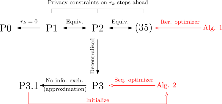
Fig. 1: Relationships between the problem formulations Section II-P3.

V Simulation Results

In this section, we present simulation studies to understand the impact of different parameters on the utility-privacy tradeoff in both the centralized (single sensor) and distributed cases. We compare our compressive privacy scheme with the IB [48], PF [50], and CP [21] privacy mechanisms. We use the following settings for all the simulations in this section (unless otherwise stated): the entries of ${\bf H}_{k}$ at each time step are drawn independently from ${\cal N}(0,1)$, ${\bf R}_{k}={\bf I}_{N}$, $\mathbf{P}_{0|0}=0.01{\bf I}_{L}$, $|\mathcal{P}|=4$, and $|\mathcal{Q}|=4$. Each data point shown in the following figures is averaged over 50 independent experiments.

V-A Centralized case

We first consider the centralized case where there is a single sensor. Recall that $\tau_{k}$ and $\eta_{k}$, which are defined in 8 and 9, denote the public error trace and private error function, respectively. The variable $r_{k}$ determines the number of future time steps that are considered in P1, and when $r_{k}=0$, only the current time step is considered. We choose 10 to be the private error function for Fig. 2 and Fig. 4 so that $|\mathcal{F}|=1$ and $\mathcal{F}(\delta\bm{1}_{|\mathcal{Q}|})=|\mathcal{Q}|\delta$. We let 11 to be the private error function for Fig. 3 so that $|\mathcal{F}|=|\mathcal{Q}|$ and $\mathcal{F}(\delta\bm{1}_{|\mathcal{Q}|})=\delta\bm{1}_{|\mathcal{Q}|}$.

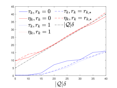
Fig. 2: The public error trace $\tau_{k}$ and privacy error trace $\eta_{k}$ vs. the privacy threshold $|\mathcal{Q}|\delta$ at $k=20$.

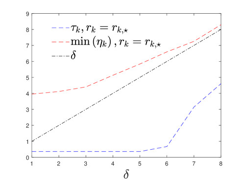
Fig. 3: The public error trace $\tau_{k}$ and the minimum of private error variances $\min(\eta_{k})$ vs. the privacy threshold $\delta$ at $k=20$ where the element-wise privacy constraint is considered and ${\bf Q}_{k}=5{\bf I}_{N}$.

Fig. 2 demonstrates the impact of $\delta$ on $\tau_{k}$ and $\eta_{k}$ with increasing $\delta$ and ${\bf Q}_{k}=2{\bf I}_{N}$. We randomly generate each $\mathbf{F}_{k}$ for all $k\geq 1$ by $\mathbf{F}_{k}=\mathbf{U}_{k}\mathbf{D}_{k}\mathbf{V}_{k}^{{}^{\intercal}}$ where $\mathbf{U}_{k}$ and $\mathbf{V}_{k}$ contain the orthonormal bases of two randomly generated matrices, and $\mathbf{D}_{k}$ is a diagonal matrix whose diagonal entries are uniformly drawn from $[1,1.2]$. The results shown are at time step $k=20$.

Recall in Algorithm 1 that we keep reducing the compression dimension $M$ until feasibility of the privacy constraint is achieved. In the case where $r_{k}$ is too small, the privacy constraint cannot be satisfied even when $M$ is reduced to 0, which implies that the information from previous time steps less than $k$ allows us to infer the private states at time $k$ better than the privacy constraint. In such a case, we set $M=0$ in our simulation result. We see from Fig. 2 that $\eta_{k}<|\mathcal{Q}|\delta$ for $r_{k}=0$ when $\delta$ is sufficiently large.

In Figs. 2 and 3, we also show the case where $r_{k}=1$ and $r_{k}=r_{k,\star}=\underset{r\geq 0}{\min}\ \left\{r:2r+\nu_{k}\geq\delta\right\}-1$ (see 25 of Proposition 1 where $\xi=1$ and $\epsilon=2$). We see that in these cases, the privacy constraint $\eta_{k}\geq|\mathcal{Q}|\delta$ is always satisfied. Moreover, we can also see in Figs. 2 and 3 that the estimation of public states is clearly compromised as $\delta$ increases.

Recall that matrices ${\bf F}_{k+n}$, for $n=0,\ldots,r_{k}$, play important roles in multi-step utility-privacy tradeoffs. To quantify the impact of ${\bf F}_{k+n}$, we let $\omega\in[0,1]$ and choose

$$\mathbf{F}_{k+n} =\left[\begin{array}[]{cc}\omega\left[{\bf F}\right]_{\cal P,P}&(1-\omega)\left[{\bf F}\right]_{\cal P,Q}\\ (1-\omega)\left[{\bf F}\right]_{\cal Q,P}&\omega\left[{\bf F}\right]_{\cal Q,Q}\end{array}\right],$$

where the entries of $\mathbf{F}$ for each $\mathbf{F}_{k+n}$ are drawn independently from ${\cal N}(0,1)$, and each row of ${\bf F}$ is normalized to have unit norm. A smaller $\omega$ means that the public and private states are more correlated in the next time step. In Fig. 4, we set $\omega=0.2$ to be small. When $r_{k}=0$, both public and private error traces evolve in a zigzag pattern and the privacy constraint $\eta_{k}\geq|\mathcal{Q}|\delta$ is violated at every other time step. This is due to the high correlation between the public states $\left[\mathbf{x}_{k}\right]_{\mathcal{P}}$ at time $k$ and the private states $\left[\mathbf{x}_{k+1}\right]_{\mathcal{Q}}$ at time $k+1$. For example, a small public error trace $\tau_{k}$ at time $k$ yields a small ${\operatorname{Tr}\left(\left[\tilde{\mathbf{P}}_{k+1|k}\right]_{\mathcal{Q},\mathcal{Q}}\right)}$ at time $k+1$, which leads to a small private error trace $\eta_{k+1}$ at time $k+1$. On the other hand, if we set $r_{k}=1$, the additional privacy constraint $\eta_{k+1}\geq|\mathcal{Q}|\delta$ ensures that $\eta_{k}\geq|\mathcal{Q}|\delta$ is feasible from $k=2$ onwards.

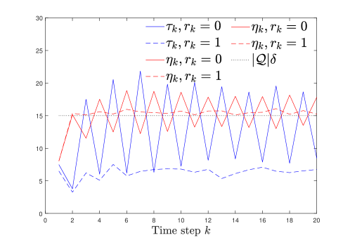
Fig. 4: The public error trace $\tau_{k}$ and private error trace $\eta_{k}$ over 20 time steps where ${\bf Q}_{k}=2{\bf I}_{N}$, $|\mathcal{Q}|\delta=15$ and $r_{k}=0,1$.

V-B Comparison amongst compressive privacy-preserving techniques

If the state and process noises in 1 are Gaussian random variables, then IB [48], PF [50], and CP [21] can be regarded as compressive privacy-preserving techniques with different utility and privacy measures. In this subsection, we briefly review these methods adapted to our problem formulation and compare them with our proposed approach, where for every time $k$, we let $r_{k}=0$ and choose the private error trace 10 as the privacy measure for our proposed approach. Since $|\mathcal{F}|=1$, we write $\gamma_{n,1}$ in 33 as $\gamma_{k}$ to use the same symbol as the tradeoff parameters of the methods we compare with.

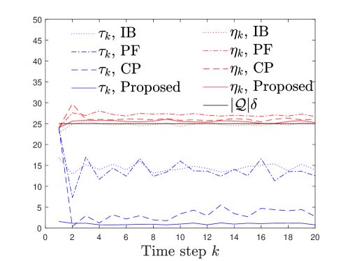
Fig. 5: Comparison of IB, PF, CP and proposed scheme in terms of $\tau_{k}$ while $\mathbf{H}_{k}$ is a random matrix and $\eta_{k}=25$. We set $\mathbf{Q}_{k}=4\mathbf{I}_{4}$ and $r_{k}=0$.

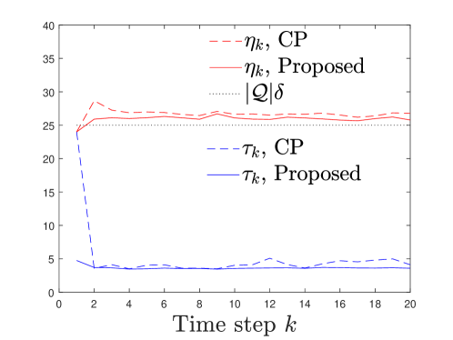
Fig. 6: Comparison of IB, PF, CP and proposed scheme in terms of $\tau_{k}$ while $\mathbf{H}_{k}$ is an orthogonal matrix and $\eta_{k}=25$. We set $\mathbf{Q}_{k}=4\mathbf{I}_{4}$ and $r_{k}=0$.

1. IB finds the optimal compressive matrix $\mathbf{C}_{k}$ by

   $$\underset{\mathbf{C}_{k}}{\min}~{}I(\mathbf{z}_{k};\mathbf{C}_{k}\mathbf{z}_{k})-\gamma_{k}I(\mathbf{C}_{k}\mathbf{z}_{k};\mathbf{y}_{k}),$$

   where $\mathbf{y}_{k}=\left[\mathbf{x}_{k}\right]_{\cal P}$ and $\gamma_{k}$ is a positive constant. The optimal compression is given by

   $$\mathbf{C}_{k}=\left[\alpha_{1}\mathbf{v}_{1},\ldots,\alpha_{M}\mathbf{v}_{M}\right]^{\intercal},$$

   where $\mathbf{v}_{i}$, for $i=1,\ldots,M$ are the left eigenvectors of

   $$\left(\mathbf{T}_{k}-\bm{\Sigma}_{z_{k},y_{k}}\left[\tilde{\mathbf{P}}_{k|k-1}\right]^{-1}_{\cal P,\cal P}\mathbf{T}_{k}\right)\mathbf{T}_{k}^{-1}$$

   with $\bm{\Sigma}_{z_{k},y_{k}}=\left[\mathbf{H}_{k}\right]_{:,\cal P}\left[\tilde{\mathbf{P}}_{k|k-1}\right]_{\cal P,P}+\left[\mathbf{H}_{k}\right]_{:,\cal Q}\left[\tilde{\mathbf{P}}_{k|k-1}\right]_{\cal Q,P}$, sorted by their corresponding ascending eigenvalues $\lambda_{1},\ldots,\lambda_{M}$, and

   $$\alpha_{i}=\sqrt{\frac{\gamma_{k}(1-\lambda_{i})-1}{\lambda_{i}\mathbf{v}_{i}^{\intercal}\mathbf{T}_{k}\mathbf{v}_{i}}}.$$

2. PF finds the optimal compressive matrix $\mathbf{C}_{k}$ by

   $$\underset{\mathbf{C}_{k}}{\max}~{}I(\mathbf{z}_{k};\mathbf{C}_{k}\mathbf{z}_{k})-\gamma_{k}I(\mathbf{C}_{k}\mathbf{z}_{k};\mathbf{y}_{k}),$$

   where $\mathbf{y}_{k}=\left[\mathbf{x}_{k}\right]_{\cal Q}$ and $\gamma_{k}$ is a positive constant. The optimal compression is given by

   $$\mathbf{C}_{k}=\left[\alpha_{1}\mathbf{v}_{1},\ldots,\alpha_{M}\mathbf{v}_{M}\right]^{\intercal},$$

   where $\mathbf{v}_{i}$, for $i=1,\ldots,M$ are the left eigenvectors of

   $$\left(\mathbf{T}_{k}-\bm{\Sigma}_{z_{k},y_{k}}\left[\tilde{\mathbf{P}}_{k|k-1}\right]^{-1}_{\cal Q,\cal Q}\mathbf{T}_{k}\right)\mathbf{T}_{k}^{-1}$$

   with $\bm{\Sigma}_{z_{k},y_{k}}=\left[\mathbf{H}_{k}\right]_{:,\cal P}\left[\tilde{\mathbf{P}}_{k|k-1}\right]_{\cal P,Q}+\left[\mathbf{H}_{k}\right]_{:,\cal Q}\left[\tilde{\mathbf{P}}_{k|k-1}\right]_{\cal Q,Q}$, sorted by their corresponding descending eigenvalues $\lambda_{1},\ldots,\lambda_{M}$.

3. CP finds the optimal $\mathbf{C}_{k}$ by

   $$\underset{\mathbf{C}_{k}}{\max}~{}I(\bm{\Gamma}^{(\mathcal{P})}_{k}\mathbf{z}_{k};\mathbf{C}_{k}\mathbf{z}_{k})-\gamma_{k}I(\bm{\Gamma}^{(\mathcal{Q})}_{k}\mathbf{z}_{k};\mathbf{C}_{k}\mathbf{z}_{k}),$$

   where $\bm{\Gamma}^{(\mathcal{P})}_{k}=\left(\left[\mathbf{H}_{k}\right]_{:,\cal Q}^{\perp}\right)^{\intercal}$ and $\bm{\Gamma}^{(\mathcal{Q})}_{k}=\left(\left[\mathbf{H}_{k}\right]_{:,\cal P}^{\perp}\right)^{\intercal}$. The optimal solution of $\mathbf{C}_{k}$ is given by

   $$\mathbf{C}_{k}^{*}=\operatorname{eig}\left(\bm{\Omega}_{k}-\gamma_{k}\bm{\Pi}_{k},\mathbf{T}_{k},M\right),$$

   where ${\rm eig}\left({\bf A},{\bf B},M\right)$ is a matrix consisting of the $M$ principal generalized unit eigenvectors of the matrix pencil $\left({\bf A},{\bf B}\right)$, and

   $$\bm{\Omega}_{k} =\mathbf{T}_{k}\left(\bm{\Gamma}^{(\mathcal{P})}_{k}\right)^{\intercal}\left(\bm{\Gamma}^{(\mathcal{P})}_{k}\mathbf{T}_{k}\left(\bm{\Gamma}^{(\mathcal{P})}_{k}\right)^{\intercal}\right)^{-1}\bm{\Gamma}^{(\mathcal{P})}_{k}\mathbf{T}_{k},$$

   $$\bm{\Pi}_{k} =\mathbf{T}_{k}\left(\bm{\Gamma}^{(\mathcal{Q})}_{k}\right)^{\intercal}\left(\bm{\Gamma}^{(\mathcal{Q})}_{k}\mathbf{T}_{k}\left(\bm{\Gamma}^{(\mathcal{Q})}_{k}\right)^{\intercal}\right)^{-1}\bm{\Gamma}^{(\mathcal{Q})}_{k}\mathbf{T}_{k}.$$

Fig. 5 and Fig. 6 compares the private error trace $\tau_{k}$ and private error trace $\eta_{k}$ of the different schemes IB, PF, CP, and our proposed approach where $r_{k}=0$. The tradeoff parameter $\gamma_{k}$ and the dimension $M$ are chosen to make $\eta_{k}$ equal to (or as close as possible to) $|\mathcal{Q}|\delta=25$ when $k$ is large. The entries of $\mathbf{F}_{k}$ are drawn independently from ${\cal N}(0,1)$, and each row of ${\bf F}_{k}$ is normalized to have unit norm. In Fig. 5 where $\mathbf{H}_{k}$ is a random matrix, we see that our proposed scheme, whose privacy metric is estimation variance, yields the lowest $\tau_{k}$ while CP yields slightly higher $\tau_{k}$ and IB and PF yield the highest $\tau_{k}$. In CP, the utility projection $\bm{\Gamma}^{(\mathcal{P})}_{k}$ and privacy projection $\bm{\Gamma}^{(\mathcal{Q})}_{k}$ cannot capture, respectively, the entire utility subspace $\left[\mathbf{H}_{k}\right]_{:,\cal P}$ and the entire privacy subspace $\left[\mathbf{H}_{k}\right]_{:,\cal Q}$, unless $\mathbf{H}_{k}$ is an orthogonal matrix. Fig. 6 shows the results when $\mathbf{H}_{k}$ is an orthogonal matrix. We see that $\tau_{k}$ in our proposed scheme is always lower than that in CP while $\eta_{k}\geq|\mathcal{Q}|\delta$ from $k=3$ onwards for both schemes.

V-C Decentralized sensors

In this subsection, we consider the case with multiple decentralized sensors. Let ${\bf Q}_{k}=4{\bf I}_{L}$, $r_{k}=r_{k,\star}$ in 25, $\delta=3$ and $N=30$. We randomly generate each $\mathbf{F}_{k}$ for all $k\geq 1$ so that its singular values are uniformly drawn from $[1,1.2]$, and use 11 as the private error function. Fig. 7 uses $S=3$ sensors and each sensor $s$’s measurement has dimension $N_{s}=N/S=10$, which is greater than the number of unknowns $L=8$, whereas Fig. 8 uses $S=5$ sensors with $N_{s}=N/S=6$, which is less than $L$ thus making each sensor an under-determined system. Comparing Fig. 7 where $N_{s}=10$ and Fig. 8 where $N_{s}=6$, we notice that the compression matrix of $N_{s}=6$ is a submatrix of the compression matrix of $N_{s}=10$. Thus, $\tau_{k}$ for $N_{s}=10$ is less than that for $N_{s}=6$. In Figs. 7 and 8, while the sequential scheme yields $\min(\eta_{k})=\delta$ for all time steps, the "no info. exch." scheme yields $\min(\eta_{k})<\delta$ thus no privacy guarantee is ensured. In Fig. 8 where each sensor is an under-determined system, the estimation errors of both public and private states are infinitely large at each sensor. Therefore, the no information exchange scheme at each sensor $s$ will choose $M_{s}$ to be $N_{s}$ for all $s=1,\ldots,S$, i.e., no compression is used. As a result, after aggregating the measurements from all sensors at fusion center, the estimation errors of both public and private states are as low as the unsanitized ones. This explains why both $\min(\eta_{k})$ and $\tau_{k}$ obtained using the no information exchange scheme are very small in Fig. 8.

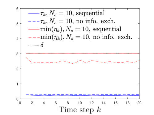
Fig. 7: The performance of the sequential scheme where $\text{Num-iter}=10$ and $N_{1},\ldots,N_{3}=10$, in terms of public error trace $\tau_{k}$ and the minimum private error variance $\min(\eta_{k})$.

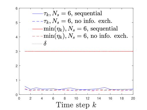
Fig. 8: The performance of the sequential scheme where $\text{Num-iter}=10$ and $N_{1},\ldots,N_{5}=6$, in terms of public error trace $\tau_{k}$ and the minimum private error variance $\min(\eta_{k})$.

Fig. 9, which uses the same settings as in Fig. 7, shows how $\tau_{k}$ and $\min(\eta_{k}(\mathbf{C}_{k}))$ evolve over the time steps $k$ for the sequential scheme. Both $\tau_{k}$ and $\min(\eta_{k}(\mathbf{C}_{k}))$ converge after a few iterations.

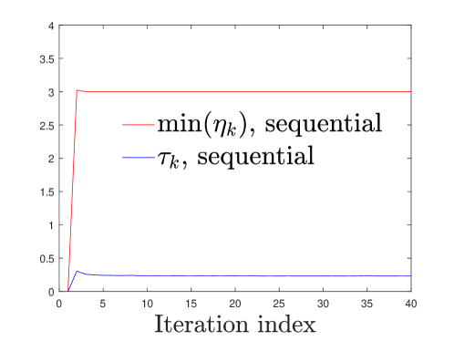
Fig. 9: Convergence of $\tau_{k}$ and $\min(\eta_{k}(\mathbf{C}_{k}))$ using Algorithm 2, where $S=3$, $N_{1},\ldots,N_{3}=10$ and $\delta=3$. The results shown are for time step $k=20$.

VI Experimental Results

VI-A Privacy-aware localization

We conduct an experiment using DecaWave UWB sensors [81] for localization. We place 5 anchor nodes at known locations $\mathbf{p}^{(A)}\in\mathbb{R}^{2\times 5}$ and estimate a mobile node’s 2-dimensional (2D) trajectory. The mobile node’s state at time $k$ is denoted as $\mathbf{x}_{k}=\left[v_{k},\theta_{k},p_{x,k},p_{y,k}\right]^{\intercal}$. The public state $\left[\mathbf{x}_{k}\right]_{\cal P}=v_{k}$ is the mobile node’s speed while the private state $\left[\mathbf{x}_{k}\right]_{\cal Q}=\left[\theta_{k},p_{x,k},p_{y,k}\right]^{\intercal}$ contains the node’s heading and 2D location. The measurements are anchor-to-mobile ranges, which are a non-linear function of the state: $\mathbf{z}_{k}=h_{k}(\mathbf{x}_{k})+\mathbf{n}_{k}$. We use the extended Kalman filter (EKF) in our estimation procedure. At each time $k$, we linearize $h_{k}$ and $f_{k}$ around the estimate $\hat{\mathbf{x}}_{k|k-1}$ and define the measurement matrix and the transition matrix, respectively, to be $\mathbf{H}_{k}=\left.\frac{\partial h_{k}(\mathbf{x})}{\partial\mathbf{x}}\right|_{\mathbf{x}=\hat{\mathbf{x}}_{k|k-1}}$ and $\mathbf{F}_{k}=\left.\frac{\partial f_{k}(\mathbf{x})}{\partial\mathbf{x}}\right|_{\mathbf{x}=\hat{\mathbf{x}}_{k-1|k-1}}$, where $f_{k}(\mathbf{x}_{k})=\left[v_{k},\theta_{k},p_{x,k}+\Delta v_{k}\cos\theta_{k},p_{y,k}+\Delta v_{k}\sin\theta_{k}\right]^{\intercal}$ with $\Delta=0.1$ being the sampling interval. The transition matrix is approximated by

$$\mathbf{F}_{k}=\left[\begin{array}[]{cccc}1&0&0&0\\ 0&1&0&0\\ \Delta\cos\hat{\theta}_{k-1}&-\Delta\sin\hat{\theta}_{k-1}\hat{v}_{k-1}&1&0\\ \Delta\sin\hat{\theta}_{k-1}&\Delta\cos\hat{\theta}_{k-1}\hat{v}_{k-1}&1&0\end{array}\right].$$

The measurement $\mathbf{z}_{k}\in\mathbb{R}^{5\times 1}$ contains range measurements between the mobile node and anchor nodes with

$$\left[\mathbf{z}_{k}\right]_{i}=\left\|\left[\mathbf{p}^{(A)}\right]_{:,i}-\left[\mathbf{x}_{k}\right]_{\cal Q}\right\|+\left[\mathbf{n}_{k}\right]_{i},i=1,\ldots,5,$$

where $\|\cdot\|$ denotes the Euclidean norm. Under the EKF framework, we let the measurement matrix $\mathbf{H}_{k}\in\mathbb{R}^{5\times 4}$ to be given by

$$\left[\mathbf{H}_{k}\right]_{i}=-\left[0,0,\frac{\left[\mathbf{p}^{(A)}\right]_{1,i}-\left[\hat{\mathbf{x}}_{k|k-1}\right]_{3}}{\left\|\left[\mathbf{p}^{(A)}\right]_{:,i}-\left[\hat{\mathbf{x}}_{k|k-1}\right]_{\cal Q}\right\|},\frac{\left[\mathbf{p}^{(A)}\right]_{2,i}-\left[\hat{\mathbf{x}}_{k|k-1}\right]_{4}}{\left\|\left[\mathbf{p}^{(A)}\right]_{:,i}-\left[\hat{\mathbf{x}}_{k|k-1}\right]_{\cal Q}\right\|}\right],\ i=1,\ldots,5,$$

where $\hat{\mathbf{x}}_{k|k-1}$ is the predicted state before measurements at time $k$. Recall that we want to protect the mobile node’s location while estimating its velocity, which however is not directly observed. In Fig. 11 and Fig. 10, we consider the centralized setting where the mobile node collects the ranging measurements and sanitizes them before sending to a server. We set $\mathbf{P}_{0}=0.01\mathbf{I}_{4}$ and $\mathbf{R}_{k}=0.04\mathbf{I}_{5},\mathbf{Q}_{k}=0.04\mathbf{I}_{4}$, and $r_{k}=0$ for all time steps $k$. The private error function used is 10.

The mobile node’s state is estimated over 318 time steps with or without compressive sanitization. We let $|\mathcal{Q}|\delta=2$. The trajectory estimated with compressive sanitization (red crosses in Fig. 10) is noticeably distorted as compared to the ground true line (black line) thus the private information is protected whereas the private information is exposed in the trajectory estimated without compressive sanitization (blue dashes), which matches the ground truth line well. On the other hand, the public information (red line in Fig. 11), i.e., the speed of the mobile node matches fairly well with the unsanitized one (black line). This experiment shows the proposed approach is also applicable to non-linear dynamical systems that can be approximated using the EKF framework.

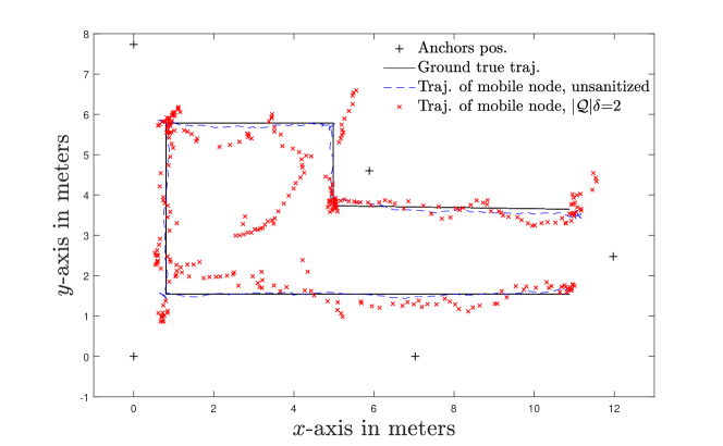
Fig. 10: Estimation of the mobile node’s locations (private states).

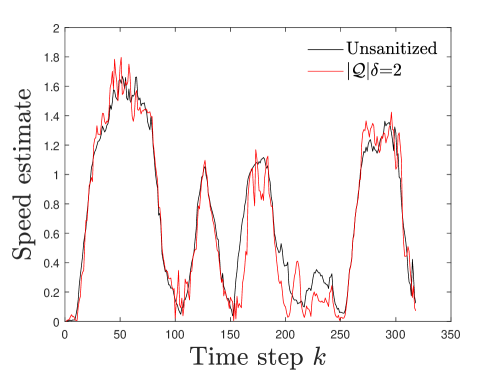
Fig. 11: Estimation of the mobile node’s speed (public states).

VI-B Privacy-aware human activity recognition

In this section, we test our approach using the public data set for human activity recognition (HAR) from [82]. We consider three activity labels: walking, walking upstairs and walking downstairs, in which walking is the public label while walking upstairs/downstairs are the private labels (e.g., these two activities can reveal how many floors the person’s house has). We evaluate the impact of all 561 features HAR provides on the public or private activity labels using 10-fold cross-validation and rank them according to information gain. This process is automated using WEKA [83]. We choose five features ($|\mathcal{P}|=5$) that have the biggest impact on walking and five features ($|\mathcal{Q}|=5$) that have the biggest impact on walking upstairs/downstairs. The public features and private features are mutually exclusive. There are 30 subjects involved in HAR. For each subject, we update all $L=10$ features successively at each time step using our approach, where we set $\mathbf{P}_{0|0}=0.01\mathbf{I}_{10}$, $\mathbf{F}_{k}=\mathbf{I}_{10},\mathbf{Q}_{k}=0.2\mathbf{I}_{10}$, and $\mathbf{H}_{k}\in\mathbb{R}^{N_{k}\times L}$ to be an identity matrix $\mathbf{I}_{L}$ with its rows being randomly dropped with probability of 0.8 at each time step to simulate lossy transmission, and $\mathbf{R}_{k}=0.1\mathbf{I}_{N_{k}}$. Fig. 12 shows the public error trace $\tau_{k}$ and private error trace $\eta_{k}$ where we choose 10 to be the private error function for Fig. 12 so that $|\mathcal{F}|=1$ and $\mathcal{F}(\delta\bm{1}_{|\mathcal{Q}|})=|\mathcal{Q}|\delta$ and $\delta=1$ and results are obtained by averaging over 30 subjects. We see that our framework is able to generate a low public error trace $\tau_{k}$ and a high private error trace $\eta_{k}$.

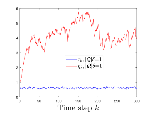
Fig. 12: The public error trace $\tau_{k}$ and private error trace $\eta_{k}$ for estimating public features and private features, respectively.

VII Conclusion

In this paper, we have investigated the use of compressive privacy schemes in a LDS to prevent the fusion center from estimating a set of private states accurately while still allowing it to estimate a set of public states with good accuracy. We developed an optimization framework to find the optimal compression matrix at each time step to achieve an optimal tradeoff between the utility at the current time step and privacy protection at multiple steps in the future. We showed that this approach allows us to ensure the same level of privacy in all future time steps in a LDS. We develop algorithms to solve for the optimal compression matrix in both the centralized and decentralized settings. For the decentralized case, we proposed the sequential update schedule. Extensive simulations are performed to verify the performance of our proposed approaches with comparisons to other methods in the literature, which are however not designed for LDS. Two empirical experiments are conducted to verify that our proposed approach on real-world time series data.

In this paper, we have not considered the case where side information at each time step may be used in privacy attacks to infer the private states. In our formulation, such initial side information can be captured in the prior distribution at time step 0. It is of interest in future research work to consider the availability of side information at every time step. Moreover, our approach is model dependent and thus accurate measurement and state models are essential for our approach.

Appendix A Proof of Lemma 2

Let $\mathbf{A}^{\prime}=\mathbf{A}\mathbf{B}^{1/2}$. Let ${\bf V}{\bf\Lambda}{\bf U}^{\intercal}$ be the truncated version of the singular value decomposition (SVD) of $\mathbf{A}^{\prime}$, where ${\bf\Lambda}\in\mathbb{R}^{M\times M}$ is a diagonal matrix with non-zero singular values being its diagonal elements, ${\bf V}\in\mathbb{R}^{M\times M}$ contains the $M$ left singular vectors, and $\mathbf{U}$ is as defined in the lemma statement. Substituting the SVD of $\mathbf{A}^{\prime}$ into the left-hand side of 28, we obtain the right-hand side. This completes the proof.

Appendix B Proof of Lemma 4

Let $\{\lambda_{\mathbf{A},i},i=1,\ldots,N\}$ and $\{\lambda_{-\mathbf{B},i},i=1,\ldots,N\}$ denote the eigenvalues of $\mathbf{A}$ and $-\mathbf{B}$, respectively, sorted in descending order. The eigenvalues of ${\bf C}$, denoted as $\{\lambda_{\mathbf{C},i},i=1,\ldots,N\}$ sorted in descending order, satisfy Weyl’s inequality:

$$\lambda_{\mathbf{A},N}+\lambda_{-\mathbf{B},i}\leq\lambda_{C,i}\leq\lambda_{\mathbf{A},i}+\lambda_{-\mathbf{B},1},i=1,\ldots,N.$$

Since $N>r_{\mathbf{A}}+r_{\mathbf{B}}$, $\lambda_{\mathbf{A},i}=0$ for $i>r_{\mathbf{A}}$ and $\lambda_{-\mathbf{B},i}=0$ for $i\leq N-r_{\mathbf{B}}$. Then, we have

$$0\leq\lambda_{\mathbf{C},i}\leq\lambda_{\mathbf{A},i}, \ 1\leq i\leq r_{\mathbf{A}},$$

$$\lambda_{\mathbf{C},i}=0, \ r_{\mathbf{A}}+1\leq i\leq N-r_{\mathbf{B}}$$

$$\lambda_{-\mathbf{B},i}\leq\lambda_{\mathbf{C},i}\leq 0, \ N-r_{\mathbf{B}}+1\leq i\leq N.$$

The proof is now complete.

Appendix C Derivation of (52)

Let ${\bm{\Pi}}_{i,j}$ be a permutation matrix that swaps the $i$th and the $j$th columns of the identity matrix ${\bf I}_{S}$. Then, right multiplying a matrix by ${\bm{\Pi}}_{s\rightarrow 1}={\bm{\Pi}}_{s,s-1}{\bm{\Pi}}_{s-1,s-2}\cdots{\bm{\Pi}}_{2,1}$ ends up moving the $s$th column of this matrix to its $1$st column and it’s easy to verify that ${\bm{\Pi}}_{s\rightarrow 1}{\bm{\Pi}}_{s\rightarrow 1}^{\intercal}=\mathbf{I}_{s}$. In what follows, we firstly show that $\mathbf{D}_{k+n|k}$ does not depend on the order of sensors and then separate the terms depending on $\left[{\bf C}_{k}\right]_{\mathcal{J}_{s},\mathcal{I}_{s}}$ in $\mathbf{D}_{k+n|k}$ from the terms depending on $\left[{\bf C}_{k}\right]_{\mathcal{J}_{\setminus s},\mathcal{I}_{\setminus s}}$. From 41, we have

$$\mathbf{D}_{k+n|k}= \left[\left[{\bf G}_{k+n|k}\right]_{\mathcal{I}_{1}}^{\intercal}\left[{\bf C}_{k}\right]^{\intercal}_{\mathcal{J}_{1},\mathcal{I}_{1}},\ldots,\left[{\bf G}_{k+n|k}\right]_{\mathcal{I}_{S}}^{\intercal}\left[{\bf C}_{k}\right]^{\intercal}_{\mathcal{J}_{s},\mathcal{I}_{s}}\right]{\bm{\Pi}}_{s\rightarrow 1}$$

$${\bm{\Pi}}_{s\rightarrow 1}^{\intercal}{\bm{\Psi}_{k}}^{-1}{\bm{\Pi}}_{s\rightarrow 1}{\bm{\Pi}}_{s\rightarrow 1}^{\intercal}\left[\begin{array}[]{c}\left[{\bf C}_{k}\right]_{\mathcal{J}_{1},\mathcal{I}_{1}}\left[{\bf G}_{k+n|k}\right]_{\mathcal{I}_{1}}\\ \vdots\\ \left[{\bf C}_{k}\right]_{\mathcal{J}_{s},\mathcal{I}_{s}}\left[{\bf G}_{k+n|k}\right]_{\mathcal{I}_{S}}\end{array}\right],$$ (56)

$$= \left[\left[{\bf G}_{k+n|k}\right]_{\mathcal{I}_{1}}^{\intercal}\left[{\bf C}_{k}\right]^{\intercal}_{\mathcal{J}_{1},\mathcal{I}_{1}},\ldots,\left[{\bf G}_{k+n|k}\right]_{\mathcal{I}_{S}}^{\intercal}\left[{\bf C}_{k}\right]^{\intercal}_{\mathcal{J}_{s},\mathcal{I}_{s}}\right]{\bm{\Pi}}_{s\rightarrow 1}$$

$$\left({\bm{\Pi}}_{s\rightarrow 1}^{\intercal}{\bm{\Psi}_{k}}{\bm{\Pi}}_{s\rightarrow 1}\right)^{-1}{\bm{\Pi}}_{s\rightarrow 1}^{\intercal}\left[\begin{array}[]{c}\left[{\bf C}_{k}\right]_{\mathcal{J}_{1},\mathcal{I}_{1}}\left[{\bf G}_{k+n|k}\right]_{\mathcal{I}_{1}}\\ \vdots\\ \left[{\bf C}_{k}\right]_{\mathcal{J}_{s},\mathcal{I}_{s}}\left[{\bf G}_{k+n|k}\right]_{\mathcal{I}_{S}}\end{array}\right],$$ (60)

$$= \left[\left[{\bf G}_{k+n|k}\right]^{\intercal}_{\mathcal{I}_{s}}\left[{\bf C}_{k}\right]^{\intercal}_{\mathcal{J}_{s},\mathcal{I}_{s}},\left[{\bf G}_{k+n|k}\right]^{\intercal}_{\mathcal{I}_{{\setminus s}}}\left[{\bf C}_{k}\right]^{\intercal}_{\mathcal{J}_{\setminus s},\mathcal{I}_{\setminus s}}\right]$$

$$\left[\begin{array}[]{cc}\left[{\bf C}_{k}\right]_{\mathcal{J}_{s},\mathcal{I}_{s}}\left[\mathbf{T}_{k}\right]_{\mathcal{I}_{s},\mathcal{I}_{s}}\left[{\bf C}_{k}\right]^{\intercal}_{\mathcal{J}_{s},\mathcal{I}_{s}}&\left[{\bf C}_{k}\right]_{\mathcal{J}_{s},\mathcal{I}_{s}}\left[\mathbf{T}_{k}\right]_{{\mathcal{I}_{s},\mathcal{I}_{\setminus s}}}\left[{\bf C}_{k}\right]^{\intercal}_{\mathcal{J}_{\setminus s},\mathcal{I}_{\setminus s}}\\ \left[{\bf C}_{k}\right]_{\mathcal{J}_{\setminus s},\mathcal{I}_{\setminus s}}\left[\mathbf{T}_{k}\right]_{{\mathcal{I}_{s},\mathcal{I}_{\setminus s}}}^{\intercal}\left[{\bf C}_{k}\right]^{\intercal}_{\mathcal{J}_{s},\mathcal{I}_{s}}&[\bm{\Phi}_{k}]_{{\mathcal{I}_{\setminus s},\mathcal{I}_{\setminus s}}}\end{array}\right]^{-1}$$ (63)

$$\left[\begin{array}[]{c}\left[{\bf C}_{k}\right]_{\mathcal{J}_{s},\mathcal{I}_{s}}\left[{\bf G}_{k+n|k}\right]_{\mathcal{I}_{s}}\\ \left[{\bf C}_{k}\right]_{\mathcal{J}_{\setminus s},\mathcal{I}_{\setminus s}}\left[{\bf G}_{k+n|k}\right]_{\mathcal{I}_{{\setminus s}}}\end{array}\right],$$ (66)

$$= \left[{\bf G}_{k+n|k}\right]_{\mathcal{I}_{s}}^{\intercal}\left[{\bf C}_{k}\right]^{\intercal}_{\mathcal{J}_{s},\mathcal{I}_{s}}\left(\left[{\bf C}_{k}\right]_{\mathcal{J}_{s},\mathcal{I}_{s}}\mathbf{T}_{k}^{(s)}\left[{\bf C}_{k}\right]^{\intercal}_{\mathcal{J}_{s},\mathcal{I}_{s}}\right)^{-1}$$

$$\left[{\bf C}_{k}\right]_{\mathcal{J}_{s},\mathcal{I}_{s}}\left[{\bf G}_{k+n|k}\right]_{\mathcal{I}_{s}}$$

$$-\left[{\bf G}_{k+n|k}\right]_{\mathcal{I}_{s}}^{\intercal}\left[{\bf C}_{k}\right]^{\intercal}_{\mathcal{J}_{s},\mathcal{I}_{s}}\left(\left[{\bf C}_{k}\right]_{\mathcal{J}_{s},\mathcal{I}_{s}}\mathbf{T}_{k}^{(s)}\left[{\bf C}_{k}\right]^{\intercal}_{\mathcal{J}_{s},\mathcal{I}_{s}}\right)^{-1}$$

$$~{}~{}~{}\left[{\bf C}_{k}\right]_{\mathcal{J}_{s},\mathcal{I}_{s}}\left[\mathbf{T}_{k}\right]_{{\mathcal{I}_{s},\mathcal{I}_{\setminus s}}}\left[{\bf C}_{k}\right]^{\intercal}_{\mathcal{J}_{\setminus s},\mathcal{I}_{\setminus s}}[\bm{\Phi}_{k}]^{-1}_{{\mathcal{I}_{\setminus s},\mathcal{I}_{\setminus s}}}\left[{\bf C}_{k}\right]_{\mathcal{J}_{\setminus s},\mathcal{I}_{\setminus s}}\left[{\bf G}_{k+n|k}\right]_{\mathcal{I}_{{\setminus s}}}$$

$$-\left[{\bf G}_{k+n|k}\right]_{\mathcal{I}_{{\setminus s}}}^{\intercal}\left[{\bf C}_{k}\right]^{\intercal}_{\mathcal{J}_{\setminus s},\mathcal{I}_{\setminus s}}[\bm{\Phi}_{k}]^{-1}_{{\mathcal{I}_{\setminus s},\mathcal{I}_{\setminus s}}}\left[{\bf C}_{k}\right]_{\mathcal{J}_{\setminus s},\mathcal{I}_{\setminus s}}\left[\mathbf{T}_{k}\right]_{{\mathcal{I}_{s},\mathcal{I}_{\setminus s}}}^{\intercal}$$

$$\left[{\bf C}_{k}\right]^{\intercal}_{\mathcal{J}_{s},\mathcal{I}_{s}}\left(\left[{\bf C}_{k}\right]_{\mathcal{J}_{s},\mathcal{I}_{s}}\mathbf{T}_{k}^{(s)}\left[{\bf C}_{k}\right]^{\intercal}_{\mathcal{J}_{s},\mathcal{I}_{s}}\right)^{-1}\left[{\bf C}_{k}\right]_{\mathcal{J}_{s},\mathcal{I}_{s}}\left[{\bf G}_{k+n|k}\right]_{\mathcal{I}_{s}}$$

$$+\left[{\bf G}_{k+n|k}\right]_{\mathcal{I}_{{\setminus s}}}^{\intercal}\left[{\bf C}_{k}\right]^{\intercal}_{\mathcal{J}_{\setminus s},\mathcal{I}_{\setminus s}}[\bm{\Phi}_{k}]^{-1}_{{\mathcal{I}_{\setminus s},\mathcal{I}_{\setminus s}}}\left[{\bf C}_{k}\right]_{\mathcal{J}_{\setminus s},\mathcal{I}_{\setminus s}}\left[\mathbf{T}_{k}\right]_{{\mathcal{I}_{s},\mathcal{I}_{\setminus s}}}^{\intercal}$$

$$\left[{\bf C}_{k}\right]^{\intercal}_{\mathcal{J}_{s},\mathcal{I}_{s}}\left(\left[{\bf C}_{k}\right]_{\mathcal{J}_{s},\mathcal{I}_{s}}\mathbf{T}_{k}^{(s)}\left[{\bf C}_{k}\right]^{\intercal}_{\mathcal{J}_{s},\mathcal{I}_{s}}\right)^{-1}\left[{\bf C}_{k}\right]_{\mathcal{J}_{s},\mathcal{I}_{s}}\left[\mathbf{T}_{k}\right]_{{\mathcal{I}_{s},\mathcal{I}_{\setminus s}}}$$

$$\left[{\bf C}_{k}\right]_{\mathcal{J}_{\setminus s},\mathcal{I}_{\setminus s}}^{\intercal}[\bm{\Phi}_{k}]^{-1}_{{\mathcal{I}_{\setminus s},\mathcal{I}_{\setminus s}}}\left[{\bf C}_{k}\right]_{\mathcal{J}_{\setminus s},\mathcal{I}_{\setminus s}}\left[{\bf G}_{k+n|k}\right]_{\mathcal{I}_{{\setminus s}}}$$

$$+\left[{\bf G}_{k+n|k}\right]_{\mathcal{I}_{{\setminus s}}}^{\intercal}\left[{\bf C}_{k}\right]^{\intercal}_{\mathcal{J}_{\setminus s},\mathcal{I}_{\setminus s}}[\bm{\Phi}_{k}]^{-1}_{{\mathcal{I}_{\setminus s},\mathcal{I}_{\setminus s}}}\left[{\bf C}_{k}\right]_{\mathcal{J}_{\setminus s},\mathcal{I}_{\setminus s}}\left[{\bf G}_{k+n|k}\right]_{\mathcal{I}_{{\setminus s}}},$$

where the last equality follows from the matrix inversion lemma. Applying Lemma 2, we obtain 52.

References

- [1] K. Sun, I. Esnala, S. M. Perlaza, and H. V. Poor, “Information-theoretic attacks in the smart grid,” in Proc. IEEE Int. Conf. Smart Grid Communications, 2017.
- [2] J. Chen, K. Kwong, D. Chang, J. Luk, and R. Bajcsy, “Wearable sensors for reliable fall detection,” in Proc. Annual Int. Conf. of the IEEE Engineering in Medicine and Biology Society, 2006, pp. 3551–3554.
- [3] W. P. Tay, J. N. Tsitsiklis, and M. Z. Win, “On the impact of node failures and unreliable communications in dense sensor networks,” IEEE Trans. Signal Process., vol. 56, no. 6, pp. 2535–2546, Jun 2008.
- [4] H. Alemdar and C. Ersoy, “Wireless sensor networks for healthcare: A survey,” Computer Networks, vol. 54, no. 15, pp. 2688–2710, 2010.
- [5] M. Yu and D. Wang, “Model-based health monitoring for a vehicle steering system with multiple faults of unknown types,” IEEE Trans. Ind. Electron., vol. 61, no. 7, pp. 3574–3586, Jul 2014.
- [6] T. Veugen and Z. Erkin, “Content-based recommendations with approximate integer division,” in Proc. IEEE Int. Conf. Acoustics, Speech, and Signal Processing, 2015.
- [7] W. P. Tay, J. N. Tsitsiklis, and M. Z. Win, “Data fusion trees for detection: Does architecture matter?” IEEE Trans. Inf. Theory, vol. 54, no. 9, pp. 4155–4168, Sep 2008.
- [8] H. Chen, B. Chen, and P. Varshney, “A new framework for distributed detection with conditionally dependent observations,” IEEE Trans. Signal Process., vol. 60, no. 3, pp. 1409–1419, Mar 2012.
- [9] M. Leng, W. P. Tay, T. Q. S. Quek, and H. Shin, “Distributed local linear parameter estimation using gaussian SPAWN,” IEEE Trans. Signal Process., vol. 63, no. 1, pp. 244–257, Jan. 2015.
- [10] W. P. Tay, “Whose opinion to follow in multihypothesis social learning? A large deviations perspective,” IEEE J. Sel. Topics Signal Process., vol. 9, no. 2, pp. 344–359, Mar 2015.
- [11] J. Ho, W. P. Tay, T. Q. S. Quek, and E. K. P. Chong, “Robust decentralized detection and social learning in tandem networks,” IEEE Trans. Signal Process., vol. 63, no. 19, pp. 5019–5032, Oct 2015.
- [12] G. W. Hart, “Nonintrusive appliance load monitoring,” Proc. IEEE, vol. 80, no. 12, pp. 1870–1891, dec 1992.
- [13] L. Sankar, S. R. Rajagopalan, S. Mohajer, and H. V. Poor, “Smart meter privacy: A theoretical framework,” IEEE Trans. Smart Grid, vol. 4, no. 2, pp. 837–846, Jun 2013.
- [14] Y. Hong, W. M. Liu, and L. Wang, “Privacy preserving smart meter streaming against information leakage of appliance status,” IEEE Trans. Information Forensics and Security, vol. 12, no. 9, pp. 2227–2241, Sep 2017.
- [15] A. Narayanan and V. Shmatikov, “Robust de-anonymization of large sparse datasets (how to break anonymity of the netflix prize dataset),” in Proc. IEEE Symp. Security and Privacy, 2008.
- [16] J. A. Calandrino, A. Kilzer, A. Narayanan, E. W. Felten, and V. Shmatikov, ““you might also like”: Privacy risks of collaborative filtering,” in Proc. IEEE Symp. Security Privacy, may 2011, pp. 231–246.
- [17] B. Hoh, T. Iwuchukwu, Q. Jacobson, M. Gruteser, A. Bayen, J.-C. Herrera, R. Herring, D. Work, M. Annavaram, and J. Ban, “Enhancing privacy and accuracy in probe vehicle based traffic monitoring via virtual trip lines,” IEEE Trans. Mobile Comput., vol. 11, no. 5, pp. 849–864, may 2012.
- [18] H. Zhang and J. Bolot, “Anonymization of location data does not work: A large-scale measurement study,” in Proc. 17th Annu. Int. Conf. Mobile Comput. and Network, 2011.
- [19] S. Gisdakis, V. Manolopoulos, S. Tao, A. Rusu, and P. Papadimitratos, “Secure and privacy-preserving smartphone-based traffic information systems,” IEEE trans. Intell. Transp. Syst., vol. 16, no. 3, pp. 1428–1438, Jun 2015.
- [20] H. Andre and J. L. Ny, “A differentially private ensemble Kalman filter for road traffic estimation,” in Proc. IEEE Int. Conf. Acoustics, Speech, and Signal Processing, 2017.
- [21] S. Y. Kung, “Compressive privacy from information estimation,” IEEE Signal Process. Mag., vol. 34, no. 1, pp. 94–112, Jan 2017.
- [22] M. Sun and W. P. Tay, “Privacy-preserving nonparametric decentralized detection,” in Proc. IEEE Int. Conf. Acoustics, Speech, and Signal Processing, 2016.
- [23] X. He and W. P. Tay, “Multilayer sensor network for information privacy,” in Proc. IEEE Int. Conf. Acoustics, Speech, and Signal Processing, 2017.
- [24] M. Sun and W. P. Tay, “Inference and data privacy in IoT networks,” in Proc. IEEE Workshop on Signal Proc. Advances in Wireless Commun., 2017.
- [25] M. Sun, W. P. Tay, and X. He, “Toward information privacy for the internet of things: A nonparametric learning approach,” IEEE Trans. Signal Process., vol. 66, no. 7, pp. 1734–1747, Dec 2018.
- [26] D. Boneh, E. J. Goh, and K. Nissim, “Evaluating 2-DNF formulas on ciphertexts,” in Proc. Int. Conf. on Theory of Cryptography, Cambridge, MA, 2005, pp. 325–341.
- [27] Y. Ishai and A. Paskin, “Evaluating branching programs on encrypted data,” in Proc. Int. Conf. on Theory of Cryptography, Berlin, Heidelberg, 2007, pp. 575–594.
- [28] C. Gentry, “Fully homomorphic encryption using ideal lattices,” in Proc. ACM Symp. on Theory of Computing, Bethesda, MD, 2009, pp. 169–178.
- [29] A. Machanavajjhala, J. Gehrke, D. Kifer, and M. Venkitasubramaniam, “L-diversity: privacy beyond k-anonymity,” in International Conference on Data Engineering, Atlanta, GA, USA, April 2006.
- [30] V. Bindschaedler, R. Shokri, and C. A. Gunter, “Plausible deniability for privacy-preserving data synthesis,” VLDB, vol. 10, no. 5, pp. 481–492, Jan. 2017.
- [31] Y. Wang, X. Wu, and H. Donghui, “Using randomized response for differential privacy preserving data collection,” in Proc. ACM SIGKDD Int. Conf. on Knowledge Discovery and Data Mining, Washington, D.C., 2003, pp. 505–510.
- [32] A. D. Sarwate and L. Sankar, “A rate-disortion perspective on local differential privacy,” in Proc. Allerton Conf. on Commun., Control and Computing, Monticello, IL, 2014, pp. 903–908.
- [33] S. Xiong, A. D. Sarwate, and N. B. Mandayam, “Randomized requantization with local differential privacy,” in Proc. IEEE Int. Conf. Acoustics, Speech, and Signal Processing, 2016.
- [34] J. Liao, L. Sankar, F. P. Calmon, and V. Y. Tan, “Hypothesis testing under maximal leakage privacy constraints,” arXiv:1701.07099, 2017.
- [35] J. C. Duchi, M. I. Jordan, and M. J. Wainwright, “Local privacy and statistical minimax rates,” in Annual Symposium on Foundations of Computer Science, Berkeley, CA, USA, Oct. 2013.
- [36] F. du Pin Calmon and N. Fawaz, “Privacy against statistical inference,” in Proc. Annual Allerton Conf. Communication, Control, and Computing, 2012.
- [37] S. Asoodeh, F. Alajaji, and T. Linder, “Privacy-aware MMSE estimation,” in Proc. IEEE Int. Symp. on Inform. Theory, 2016.
- [38] C. Dwork and A. Roth, “The algorithmic foundations of differential privacy,” Foundations and Trends ® in Theoretical Computer Science, vol. 9, no. 3-4, pp. 211–407, 2014.
- [39] P. Cuff and L. Yu, “Differential privacy as a mutual information constraint,” in ACM SIGSAC Conference on Computer and Communications Security, October 2016, pp. 43–54.
- [40] A. Ghosh and R. Kleinberg, “Inferential privacy guarantees for differentially private mechanisms,” arXiv preprint arXiv:1603.01508, 2016.
- [41] X. He, A. Machanavajjhala, and B. Ding, “Blowfish privacy: tuning privacy-utility trade-offs using policies,” in SIGMOD, Snowbird, Utah, USA, June 2014, pp. 1447–1458.
- [42] W. Wang, L. Ying, and J. Zhang, “On the relation between identifiability, differential privacy, and mutual-information privacy,” IEEE Trans. Inf. Theory, vol. 62, pp. 5018–5029, Sep 2016.
- [43] J. C. Duchi, M. I. Jordan, , and M. J. Wainwright, “Privacy aware learning,” Journal of the ACM, vol. 61, no. 6, Nov. 2014.
- [44] S. Salamatian, A. Zhang, F. du Pin Calmon, S. Bhamidipati, N. Fawaz, B. Kveton, P. Oliveira, and N. Taft, “How to hide the elephant-or the donkey-in the room: Practical privacy against statistical inference for large data,” in Proc. IEEE Global Conf. on Signal and Information Processing, Austin, TX, no. 269-272, 2013.
- [45] H. Yamamoto, “A source coding problem for sources with additional outputs to keep secret from the receiver or wiretappers,” IEEE Trans. Inf. Theory, vol. 29, no. 6, pp. 918–923, Nov 1983.
- [46] A. Globerson, G. Chechik, and N. Tishby, “Extracting continuous relevant features,” in Proc. Annual Conf. of the Gesellschaft für Klassifikation e.V., Brandenburg, 2003, pp. 224–238.
- [47] G. Chechik and N. Tishby, “Extracting relevant structures with side information,” in Advances in Neural Information Processing Systems, 2002, pp. 857–864.
- [48] G. Chechik, A. Globerson, N. Tishby, and Y. Weiss, “Information bottleneck for gaussian variables,” in Advances in Neural Information Processing Systems, 2003.
- [49] A. Emad and O. Milenkovic, “Compression of noisy signals with information bottlenecks,” in Proc. IEEE Information Theory Workshop, 2013.
- [50] A. Makhdoumi, S. Salamatian, and N. Fawaz, “From the information bottleneck to the privacy funnel,” in Proc. IEEE Information Theory Workshop, 2014.
- [51] K. Diamantaras and S. Kung, “Data privacy protection by kernel subspace projection and generalized eigenvalue decomposition,” in IEEE Int. Workshop Machine Learning for Signal Processing, Salerno, 2016, pp. 1–6.
- [52] S. Y. Kung, “A compressive privacy approach to generalized information bottleneck and privacy funnel problems,” Journal of the Franklin Institute, Jul 2017.
- [53] M. Al, S. Wan, and S. Kung, “Ratio utility and cost analysis for privacy preserving subspace projection,” arXiv preprint arXiv:1702.07976, 2017.
- [54] T. Chanyaswad, J. M. Chang, P. Mittal, and S. Y. Kung, “Discriminant-component eigenfaces for privacy-preserving face recognition,” in International Workshop on Machine Learning for Signal Processing, Vietri sul Mare, Italy, Sept. 2016.
- [55] S. Y. Kung, T. Chanyaswad, J. M. Chang, and P. Wu, “Collaborative pca/dca learning methods for compressive privacy,” ACM T EMBED COMPUT S., vol. 16, no. 3, 2017.
- [56] T. Chanyaswad, J. M. Chang, and S. Y. Kung, “A compressive multi-kernel method for privacy-preserving machine learning,” in International Joint Conference on Neural Networks, Anchorage, AK, USA, May 2017.
- [57] J. L. Ny and G. J. Pappas, “Differentially private filtering,” IEEE Trans. Automat. Contr., vol. 59, pp. 341–354, Feb 2014.
- [58] K. H. Degue and J. L. Ny, “On differentially private Kalman filtering,” in Proc. IEEE Global Conf. on Signal and Information Processing, 2017.
- [59] C. Dwork, K. Kenthapadi, F. McSherry, I. Mironov, and M. Naor, “Our data, ourselves: Privacy via distributed noise generation,” EUROCRYPT, pp. 486–503, 2006.
- [60] M. Stein, M. Castañeda, and A. Mezghani, “Information-preserving transformations for signal parameter estimation,” IEEE Signal Processing Letters, vol. 21, no. 7, pp. 866–870, Jul 2014.
- [61] Y. Song, C. X. Wang, and W. P. Tay, “Privacy-aware Kalman filtering,” in Proc. IEEE Int. Conf. Acoustics, Speech, and Signal Processing, Calgary, Canada, 2018.
- [62] D. Reid, “An algorithm for tracking multiple targets,” IEEE Trans. Automat. Contr., vol. 24, no. 6, pp. 843–854, Dec. 1979.
- [63] S. J. Julier and J. K. Uhlmann, “Unscented filtering and nonlinear estimation,” Proc. IEEE, vol. 92, no. 3, pp. 401–422, Mar. 2004.
- [64] S. Huang and G. Dissanayake, “Convergence analysis for extended Kalman filter based SLAM,” IEEE Trans. Robot., vol. 23, no. 5, pp. 1036–1049, October 2007.
- [65] B. Sinopoli, L. Schenato, M. Franceschetti, K. Poolla, M. I. Jordan, and S. S. Sastry, “Kalman filtering with intermittent observations,” IEEE Trans. Automat. Contr., vol. 49, no. 9, pp. 1453–1464, Sep. 2004.
- [66] L. Schenato, B. Sinopoli, M. Franceschetti, K. Poolla, and S. S. Sastry, “Foundations of control and estimation over lossy networks,” Proceedings of the IEEE, vol. 95, no. 1, pp. 163–187, Jan. 2007.
- [67] M. C. F. Donkers, W. P. M. H. Heemels, N. van de Wouw, and L. Hetel, “Stability analysis of networked control systems using a switched linear systems approach,” IEEE Trans. Automat. Contr., vol. 56, no. 9, pp. 2101–2115, Sep. 2011.
- [68] Y. Xia, J. Shang, J. Chen, , and G.-P. Liu, “Networked data fusion with packet losses and variable delays,” IEEE Trans. Syst. Man Cybern. - Part B: Cybern., vol. 39, no. 5, pp. 1107–1120, October 2009.
- [69] X. Liu and A. Goldsmith, “Kalman filtering with partial observation losses,” in IEEE Conference on Decision and Control, December 2004.
- [70] M. Huang and S. Dey, “Stability of kalman filtering with markovian packet losses,” Automatica, vol. 43, pp. 598–607, 2007.
- [71] Y. Liang, T. Chen, and Q. Pan, “Optimal linear state estimator with multiple packet dropouts,” IEEE Trans. Automat. Contr., vol. 55, no. 6, pp. 1428–1433, June 2010.
- [72] Y. Mo and B. Sinopoli, “Kalman filtering with intermittent observations: Tail distribution and critical value,” IEEE Trans. Automat. Contr., vol. 57, no. 3, pp. 677–689, March 2012.
- [73] M. Nourian, A. S. Leong, and S. Dey, “Optimal energy allocation for kalman filtering over packet dropping links with imperfect acknowledgments and energy harvesting constraints,” IEEE Trans. Automat. Contr., vol. 59, no. 8, pp. 2128–2143, August 2014.
- [74] M. Sahebsara, T. Chen, and S. L. Shah, “Optimal h2 filtering in networked control systems with multiple packet dropout,” IEEE Trans. Automat. Contr., vol. 52, no. 8, pp. 1508–1513, August 2007.
- [75] L. Shi, M. Epstein, and R. M. Murray, “Kalman filtering over a packet-dropping network: A probabilistic perspective,” IEEE Trans. Automat. Contr., vol. 55, no. 3, pp. 594–604, March 2010.
- [76] E. I. Silva and M. A. Solis, “An alternative look at the constant-gain kalman filter for state estimation over erasure channels,” IEEE Trans. Automat. Contr., vol. 58, no. 2, pp. 3259–3265, December 2013.
- [77] S. Kar and J. M. F. Moura, “Gossip and distributed kalman filtering: Weak consensus under weak detectability,” IEEE Trans. Signal Process., vol. 59, no. 4, pp. 1766–1784, April 2011.
- [78] D. E. Quevedo, A. Ahlén, and K. H. Johansson, “State estimation over sensor networks with correlated wireless fading channels,” IEEE Trans. Automat. Contr., vol. 58, no. 3, pp. 581–593, March 2013.
- [79] E. R. Rohr, D. Marelli, and M. Fu, “Kalman filtering with intermittent observations: On the boundedness of the expected error covariance,” IEEE Trans. Automat. Contr., vol. 59, no. 10, pp. 2724–2738, October 2014.
- [80] R. E. Kalman, “A new approach to linear filtering and prediction problems,” J. of Basic Eng., vol. 82, no. 1, pp. 35–45, Mar 1960.
- [81] https://www.decawave.com/.
- [82] D. Anguita, A. Ghio, L. Oneto, X. Parra, and J. L. Reyes-Ortiz, “A public domain dataset for human activity recognition using smartphones,” in 21th European Symposium on Artificial Neural Networks, Computational Intelligence and Machine Learning, Bruges, Belgium, April 2013.
- [83] E. Frank, M. A. Hall, and I. H. Witten, The WEKA Workbench. Online Appendix for "Data Mining: Practical Machine Learning Tools and Techniques". Morgan Kaufmann, Fourth Edition, 2016.