A global sensitivity analysis and reduced order models
for hydraulically-fractured horizontal wells
   
An e-print of the paper will be made available on arXiv.

Authored by
Ali Rezaei, Postdoctoral Research Associate

Department of Petroleum Engineering
University of Houston, Houston, Texas 77204–4003
phone: +1-651-245-7918, e-mail: arezaei2@uh.edu

Kalyana B. Nakshatrala, Associate Professor

Department of Civil & Environmental Engineering
University of Houston, Houston, Texas 77204–4003.
phone: +1-713-743-4418, e-mail: knakshatrala@uh.edu
website: http://www.cive.uh.edu/faculty/nakshatrala

Fahd Siddiqui, Postdoctoral Research Associate

Department of Petroleum Engineering
University of Houston, Houston, Texas 77204–4003
phone: +1-713-743-6103, e-mail: fsiddiq6@central.uh.edu

Birol Dindoruk, Professor

Department of Petroleum Engineering
University of Houston & Shell International Exploration and Production Inc., Houston, Texas 77204–4003
phone: +1-832-875-9092, e-mail: birol.dindoruk@shell.com

Mohammed Soliman, Professor

Department Chair and William C. Miller Endowed Chair Professor
Department of Petroleum Engineering
University of Houston, Houston, Texas 77204–4003
phone: +1-713-743-6103, e-mail: msoliman@central.uh.edu

2018
Computational and Applied Mechanics Laboratory

Abstract.

Several factors affect the performance and stimulation design of hydraulically-fractured wells. Moreover, the dominant factors vary for different quantities of interest, and vary based on the spatial location and with the time of interest. Thus, it will be beneficial if there is a systematic procedure to identify the dominant factors affecting the quantities of interest. To this end, we present a systematic global sensitivity analysis using the Sobol method which can be utilized to rank the variables that affect two quantity of interests – pore pressure depletion and stress change – around a hydraulically-fractured horizontal well based on their degree of importance. These variables include rock properties and stimulation design variables. A fully-coupled poroelastic hydraulic fracture model is used to account for pore pressure and stress changes due to production. To ease the computational cost of a simulator, we also provide reduced order models (ROMs), which can be used to replace the complex numerical model with a rather simple analytical model, for calculating the pore pressure and stresses at different locations around hydraulic fractures. The two main reason for choosing the Sobol method are that it can capture the individual and interaction effects of input variables on the variance of outputs (which is not the case with local sensitivity analysis techniques). It also furnishes a systematic procedure with strong mathematical underpinning to generate ROMs for various quantities of interests for a given mathematical model and for a given set of input variables. The main findings of this research are: (i) mobility, production pressure, and fracture half-length are the main contributors to the changes in the quantities of interest. The percentage of the contribution of each parameter depends on the location with respect to pre-existing hydraulic fractures and the quantity of interest. (ii) As the time progresses, the effect of mobility decreases and the effect of production pressure increases. (iii) These two variables are also dominant for horizontal stresses at large distances from hydraulic fractures. (iv) At zones close to hydraulic fracture tips or inside the spacing area, other parameters such as fracture spacing and half-length are the dominant factors that affect the minimum horizontal stress. The results of this study will provide useful guidelines for the stimulation design of legacy wells and secondary operations such as refracturing and infill drilling.

1. INTRODUCTION AND MOTIVATION

Horizontal wells that are drilled in unconventional reservoirs typically show a decline in their initial production rate (IPR) over time. Multiple hydraulic fractures are usually placed in these wells towards the completion stage to enable the production of hydrocarbons. These fractures create high permeability conduits which allow the flow of hydrocarbons from the rock matrix to the well. In some of these wells, production rate drops below the non-economical threshold which places these wells at the risk of abandonment. The drop in the production rate is mainly due to the small drainage area of these low permeability reservoirs that is limited to the inner reservoir between the fractures (Ozkan et al, 2009). It can also have other sources such as proppant degradation and un-successful initial stimulation. Possible ways of increasing the production from these reservoirs are to re-fracture the horizontal well after the occurrence of the production decline, or drill an infill well parallel to the current well and stimulate it. These methods enable production from a bypassed, or intact area of the reservoir. A problem that exists while doing these practices is the redistribution of stresses in the depleted area of the reservoir that might be in the vicinity of a newly created hydraulic fracture. This redistribution of stress causes the new fractures to behave differently than the initial fractures and sometimes failing in the re-stimulation attempts. Therefore, several factors such as extent and severity of the pore pressure depletion have to be considered while designing a refracturing, or an infill fracturing process.

Hydraulic fracturing design plays a critical role in the success of any refracturing and infill well fracturing process. Several factors such as the state of in-situ stresses, rock geomechanical properties, operation variables (e.g., pump rate, proppant concentration) should be considered in such a design. The host medium with hydraulic fractures can be considered as a fully-saturated poroelastic rock. Hence, in order to properly study the process of placing hydraulic fractures into the formation that contains pre-existing fractures with a depleted area in their vicinity, the strong coupling between pore pressure and rock deformation should be taken into account. It is demonstrated that the pore pressure change (which is caused by production or injection) redistributes the stress state of the rock in the vicinity of hydraulic fractures (Berchenko and Detournay, 1997; Roussel and Sharma, 2012; Safari et al, 2015; Rezaei et al, 2017a, b, 2018). The stress redistribution affects further activities such as refracturing and infill well fracturing by affecting the preferred propagation direction of fractures either in the same well or an off-set well. Thus, it is crucial to understand the main variables that contribute to the stress redistribution.

Sensitivity analysis (SA) is a method for quantifying the importance of each model input parameter on the value of a model output parameter. This method may be used to identify the key input parameters whose variance affects the output parameters the most. Moreover, it can be used to build a computationally faster model than the original model (Welch et al, 1992). Depending on the application, many methods have been introduced to perform such an analysis (e.g., Hill and Tiedeman, 2006; Sobol, 2001). A review on the recent advances on sensitivity analysis techniques may be found in (Iooss and Lemaître, 2015; Pianosi et al, 2016; Borgonovo and Plischke, 2016).

Generally, these methods may be categorized into two subsets, namely local and global sensitivity analysis (Saltelli et al, 2004, 2008). Global SA is a method to study the effect of the entire input parameters on the output parameters uncertainty, whereas in local SA the focus is on the output parameters themselves rather than their uncertainties. This method can be categorized into four sub-categories: regression-based, screening based, variance-based, and meta-model sensitivity analysis (Tian, 2013). Sobol (1993, 2001) developed a global SA method for calculating the individual input variable influences on the output of a complicated mathematical model. This method is used in this study to analyze and rank the influencing parameters that affect the performance of a refracturing or infill well fracturing.

Several parameters affect the changes in pore pressure around horizontal wells. These factors include rock geomechanical properties, operational variables such as production rate (or pressure), HF design parameters such as spacing and half lengths of the pre-existing hydraulic fractures, well spacing (in the case of infill well fracturing), and reservoir in-situ properties such as initial pore pressure. Identifying the parameters that have the greatest impact on the pore pressure depletion extension and magnitude (subsequently principal stresses magnitude and direction) helps to make better decisions about time and design of refracturing and infill well fracturing. Because of the large uncertainty in reservoir rocks properties, sensitivity analysis is being used repeatedly in oil and gas industry for purposes such as matching production history (rate or pressure) (Oliver and Chen, 2011), optimizing operation parameters (Yu et al, 2014), and forecast analysis (Nashawi et al, 2010). Verde (2015) used global sensitivity analysis to investigate the effect of shear modulus, Poisson’s ratio, normal joint stiffness, and minimum horizontal stress on the fluid pressure in an injector well and a producer well. They concluded that shear modulus, normal joint stiffness, minimum horizontal stress, and Poisson’s ratio have the greatest sensitivity indices respectively. Dai et al (2014) used a global sensitivity analysis based on polynomial chaos expansions (PCEs) proposed a global SA based on the uncertain parameters that were used in a reservoir simulator. Yu et al (2014) performed a local sensitivity analysis on shale gas to optimize hydraulic fracture half-length and spacing. Westwood et al (2017) applied a Monte-Carlo approach to study the effect of flow rate, pumping time, and differential pressure on the distance of the fluid penetration, stimulated rock volume (SRV), and minimum distance to avoid reactivation of the fault.

In this paper, our aim is to first show the sensitivity of pore pressure and stresses changes to rock properties, operation variables, and design parameters. Then, we use a global sensitivity scheme to study the uncertainty that is involved in the geomechanical and in-situ variables. Using this approach, parameters are indexed by their importance on the variation of pore pressure and stresses at an arbitrary point inside the rock. It also has the advantage of capturing both individuals and interaction effects of the parameters that are involved in the problem. This approach helps operators to select design parameters in a way to avoid the occurrence of problems such as stress reversal that may negatively affect any refracturing or infill well fracturing. Finally, we use Sobol method to present a reduced order model for points around hydraulically-fractured well at different times from production.

The rest of this paper is organized as follows. Section 2 provides the necessary theoretical background, which includes the presentation of a fully-coupled poroelastic hydraulic fracture model and a brief description of the Sobol method. Uncertainty of the pore pressure and stresses concerning rock type variables is given in Section 3. Global sensitivity analysis based on Sobol method is represented in Section 4 to index the variables in order of their significance concerning the pore pressure. In Section 5, using the dominant Sobol indices, reduced order models for pore pressure and stress are developed at different locations around hydraulic fractures. Finally, conclusions are drawn in Section 6.

2. THEORETICAL BACKGROUND

Our work hinges on poroelasticity, the displacement discontinuity method and the Sobol method. These ingredients are briefly described below for the benefit of the reader and for future referencing.

2.1. Poroelasticity

A poroelastic medium can be characterized by five independent material properties: the shear modulus $G$, the drained Poisson’s ratio $\nu$, the undrained Poisson’s ratio $\nu_{u}$, the Skempton’s pore pressure coefficient $B$, and the permeability coefficient $\kappa$ (Cleary, 1977; Detournay and Cheng, 1987), which we refer to mobility in this paper. The Skempton’s coefficient is defined as the ratio between the induced pore pressure and the variation of the confining pressure under the undrained condition, and the permeability coefficient is defined as the ratio between the rock permeability $k$ and the dynamic fluid viscosity $\mu$ (i.e., $\kappa=k/\mu$). Other parameters such as rock diffusion coefficient $c$ and Biot’s coefficient $\alpha$ can be derived from these independent variables as follows:

$$c=\frac{2\kappa B^{2}G(1-\nu)(1+\nu_{u})^{2}}{9(1-\nu_{u})(\nu_{u}-\nu)}\,.$$ (2.1)

$$\alpha=\frac{3(\nu_{u}-\nu)}{B(1-2\nu)(1+\nu_{u})}=1-\frac{K_{m}}{K_{s}}\,,$$ (2.2)

where $K_{s}$ and $K_{m}$ are the solid and porous matrix bulk moduli, respectively. The response of a poroelastic medium is governed by four sets of equations, which are referred to as the field equations. The four sets of equations are constitutive relations, force-equilibrium equations, Darcy’s law, and continuity equation (Biot, 1941; Cleary, 1977). Constitutive equations relate stress, strain, and pore pressure. Unlike elastic media (which need one constitutive relation), two constitutive relations are needed for poroelasticity. Of course, the field equations should be augmented with appropriate boundary and initial conditions.

A brief formulation of the generalized equations of poroelasticity are in order. We denote a spatial point by $\mathbf{x}$. The gradient and divergence operators with respect to $\mathbf{x}$ are, respectively, denoted by $\mathrm{grad}[\cdot]$ and $\mathrm{div}[\cdot]$. The Laplacian differential operator is denoted by $\Delta$. That is, $\Delta(\cdot)=\mathrm{div}[\mathrm{grad}[\cdot]]$. We denote the displacement field by $\mathbf{u}$ and also time of an arbitrary variable $a$ by $\dot{a}$. We employ linearized strain, which is defined as follows:

$$\mathbf{E}_{l}=\frac{1}{2}\left(\mathrm{grad}[\mathbf{u}]+\mathrm{grad}[\mathbf{u}]^{\mathrm{T}}\right)$$ (2.3)

Note that the strain is a second-order tensor. The volumetric strain is given by $\mathrm{tr}[\mathbf{E}_{l}]$, where $\mathrm{tr}[\cdot]$ denotes the trace of a second-order tensor (Chadwick, 2012). These equations for the case of plane strain quasi-static poroelasticity can be written as follows:

$$G\Delta(\mathbf{\mathbf{u}})+\left\{\frac{G}{1-2\nu_{u}}\right\}\mathrm{grad}[\mathrm{tr}[\mathbf{E}_{l}]]-\left\{\frac{2GB(1+\nu_{u})}{3(1-2\nu_{u})}\right\}\mathrm{grad}[\zeta]+\mathbf{f_{b}}= \;0$$ (2.4)

$$\dot{\zeta}-c\;\Delta(\zeta)-\left\{\frac{\kappa B(1+\nu_{u})}{3(1-\nu_{u})}\right\}\mathrm{div}[\mathbf{f_{b}}]+\kappa\;\mathrm{div}[\mathbf{f_{f}}]-\mathbf{\gamma}= \;0$$ (2.5)

where $\zeta$ is the variation of fluid content defined as the increment of fluid volume per unit volume of the porous medium (Biot, 1941). Moreover, $\mathbf{f_{b}}$ and $\mathbf{f_{f}}$ are the bulk and fluid body forces, respectively, $\gamma$ is the volume rate of injection from the fluid source. It should be noted that we employ mechanics convention – tensions are treated as positive and pore pressure is positive in compression. Eq. (2.4) is referred to as the Navier equation of poroelasticity (Cleary, 1977; Cheng, 2016). The two main assumptions in the deriving Equations (2.4)–(2.5) are as follows:

1. the fracturing fluid and the reservoir the fluid has the same rheology, and

2. the deformation in the rock occurs in a quasi-static plane strain condition.

Equations (2.4) and (2.5) form the building blocks of the poroelastic displacement discontinuity method (DDM). Cleary (1977) presented fundamental solutions of point force and point fluid source for the theory of poroelasticity, and Curran and Carvalho (1987) and Detournay and Cheng (1987) developed displacement discontinuity solutions of a poroelastic medium using these equations.

2.2. The poroelastic displacement discontinuity method

In this section we describe the Poroelastic Displacement Discontinuity Method (PDDM) that is used in this work. This method belongs to the class of boundary element methods (BEM), which are suitable discretization for problems in which the ratio of volume to the surface is high. Several authors used BEM for solving fracture mechanics problems (Aliabadi and Rooke, 1991; Aliabadi, 2002; Cruse, 2012). A special indirect boundary element method for the case of a line crack in an infinite medium was developed by Crouch (1976). This method is based on considering the fracture as a line in 2D (or a surface in 3D) along which one defines quantities that take into account the discontinuity in displacements from one side of the fracture to the other. Liu and Li (2014) explicitly showed that for problems involving a fracture, both DDM and BEM are equivalent. In its original formulation, DDM is based on the fundamental solutions of a point source in an infinite linear elastic medium. These fundamental solutions may be derived from dislocation theory (Bobet and Mutlu, 2005). On the other hand, in a poroelastic medium hydraulic fractures may be seen as a manifold across which a discontinuity takes place not only in the rock displacement but also in the fluid flux. We define three discontinuity fields with respect to a local coordinate system $(s,n)$ (Figure 1) as

$$D_{s}(s,n,t)=\lim_{n\rightarrow 0-}u_{s}(s,n,t)-\lim_{n\rightarrow 0+}u_{s}(s,n,t)\,,\\$$ (2.6a)

$$D_{n}(s,n,t)=\lim_{n\rightarrow 0-}u_{n}(s,n,t)-\lim_{n\rightarrow 0+}u_{n}(s,n,t)\,,\\$$ (2.6b)

$$D_{q}(s,n,t)=\dfrac{q_{0}}{2\,a\,}\,.$$ (2.6c)

Here, $D_{s}$ and $D_{n}$ denote the shear and normal displacement discontinuity fields, and $D_{q}$ is the flux discontinuity field. These fields physically represent the discontinuities in the displacements and the flow determined by a fracture. Also, $u_{s}$ and $u_{n}$ are the shear and normal components of the displacement field $\mathbf{u}$ in the local coordinate system and $q_{0}$ is the total flow injection, The above definition implies that a fracture opening corresponds to a negative $D_{n}$ and counterclockwise movement of the fracture surfaces gives a positive $D_{s}$. Also, the fluid flow is assumed to be negative if its direction is different from the chosen positive direction of total injection. Notice that the original displacement discontinuity method developed by Crouch (1976) does not have the $D_{q}$ term since it was only developed using elastic solutions with no effect of poroelasticity.

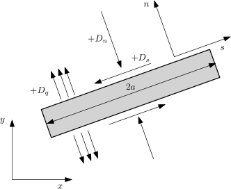
Figure 1. Definition of the shear, normal and flow discontinuities on a fracture element (the convention on the positive verses is shown)

In order to solve for displacement and flux discontinuities, we start from the integral equations relating such discontinuities to stresses and pore pressure in infinite domains (Detournay and Cheng, 1987; Vandamme et al, 1989), which read for $i,j=1,2$ (here, summation over repeated indices is used except for the indices $s,n,q$)

$$\sigma_{ij}(\mathbf{x},t)= \int_{0}^{t}\int_{\Gamma}Q_{ik}(\mathbf{\chi})Q_{jl}(\mathbf{\chi})S_{s,kl}(\mathbf{x},\mathbf{\chi};t-\tau)D_{s}(\mathbf{\chi},\tau)d\Gamma(\mathbf{\chi})d\tau$$

$$+ \int_{0}^{t}\int_{\Gamma}Q_{ik}(\mathbf{\chi})Q_{jl}(\mathbf{\chi})S_{n,kl}(\mathbf{x},\mathbf{\chi};t-\tau)D_{n}(\mathbf{\chi},\tau)d\Gamma(\mathbf{\chi})d\tau$$

$$+ \int_{0}^{t}\int_{\Gamma}Q_{ik}(\mathbf{\chi})Q_{jl}(\mathbf{\chi})S_{q,kl}(\mathbf{x},\mathbf{\chi};t-\tau)D_{q}(\mathbf{\chi},\tau)d\Gamma(\mathbf{\chi})d\tau\,,$$ (2.7a)

$$p(\mathbf{x},t)= \int_{0}^{t}\int_{\Gamma}P_{s}(\mathbf{x},\mathbf{\chi};t-\tau)D_{s}(\mathbf{\chi},\tau)d\Gamma(\mathbf{\chi})d\tau$$

$$+ \int_{0}^{t}\int_{\Gamma}P_{n}(\mathbf{x},\mathbf{\chi};t-\tau)D_{n}(\mathbf{\chi},\tau)d\Gamma(\mathbf{\chi})d\tau$$

$$+ \int_{0}^{t}\int_{\Gamma}P_{q}(\mathbf{x},\mathbf{\chi};t-\tau)D_{q}(\mathbf{\chi},\tau)d\Gamma(\mathbf{\chi})d\tau\,.$$ (2.7b)

Equations (2.7) and (2.7) are analytical solutions over the plane, where the influence functions $S_{s,kl}$, $S_{n,kl}$, $S_{q,kl}$, $P_{s}$, $P_{n}$, $P_{q}$ are given in Vandamme et al (1989) and Carvalho (1991). The influence functions give the solution of a point source or displacement discontinuity from influencing point $\mathbf{\chi}$ and at time $\tau$ on a the influencing point $\mathbf{x}$ at time $t$. Matrix $\mathbf{Q}$ represents the rotation from the local crack coordinate system to the global coordinate system.

Equations (2.7) and (2.7) form a set of integral equations for the unknown fields $D_{s}$, $D_{n}$ and $D_{q}$ with given fields $\sigma_{s}$, $\sigma_{n}$ and $p$. They show that stresses and pore pressures are obtained as a time integral that contains an integral over the fracture $\Gamma$. The discretization of the integral equations using constant spatial and constant temporal elements may be written as

$$\sum\limits_{\lambda=1}^{N}A_{xx}^{\beta\lambda}D_{s}^{\lambda,h}+\sum\limits_{\lambda=1}^{N}A_{xy}^{\beta\lambda}D_{n}^{\lambda,h}+\sum\limits_{\lambda=1}^{N}A_{xq}^{\beta\lambda}D_{q}^{\lambda,h}=$$

$$\sigma_{s}^{h}(x^{\beta},t)-\sum\limits_{\eta=0}^{h-1}\sum\limits_{\lambda=1}^{N}\bigg{(}A_{xx}^{\beta\lambda,\eta}D_{s}^{\lambda,\eta}+A_{xy}^{\beta\lambda,\eta}D_{n}^{\lambda,\eta}+A_{xq}^{\beta\lambda,\eta}D_{q}^{\lambda,\eta}\bigg{)},$$ (2.8a)

$$\sum\limits_{\lambda=1}^{N}A_{yx}^{\beta\lambda}D_{s}^{\lambda,h}+\sum\limits_{\lambda=1}^{N}A_{yy}^{\beta\lambda}D_{n}^{\lambda,h}+\sum\limits_{\lambda=1}^{N}A_{yq}^{\beta\lambda}D_{q}^{\lambda,h}=$$

$$\sigma_{n}^{h}(x^{\beta},t)-\sum\limits_{\eta=0}^{h-1}\sum\limits_{\lambda=1}^{N}\bigg{(}A_{yx}^{\beta\lambda,\eta}D_{s}^{\lambda,\eta}+A_{yy}^{\beta\lambda,\eta}D_{n}^{\lambda,\eta}+A_{yq}^{\beta\lambda,\eta}D_{q}^{\lambda,\eta}\bigg{)},$$ (2.8b)

$$\sum\limits_{\lambda=1}^{N}A_{px}^{\beta\lambda}D_{s}^{\lambda,h}+\sum\limits_{\lambda=1}^{N}A_{py}^{\beta\lambda}D_{n}^{\lambda,h}+\sum\limits_{\lambda=1}^{N}A_{pq}^{\beta\lambda}D_{q}^{\lambda,h}=$$

$$p_{p}^{h}(x^{\beta},t)-\sum\limits_{\eta=0}^{h-1}\sum\limits_{\lambda=1}^{N}\bigg{(}A_{px}^{\beta\lambda,\eta}D_{s}^{\lambda,\eta}+A_{py}^{\beta\lambda,\eta}D_{n}^{\lambda,\eta}+A_{pq}^{\beta\lambda,\eta}D_{q}^{\lambda,\eta}\bigg{)}.$$ (2.8c)

In Equations (2.8)–(2.8), $A_{ij}$ are the coefficients relating the displacement discontinuities and fluid sources to shear stress, normal stress and pore pressure. For example, $A_{xx}^{\beta\lambda,\eta}$ is the shear stress that is induced on the observation point $\beta$ from a unit shear displacement discontinuity at the source point $\lambda$ during time $\eta$, where $\eta$ is the time between occurrence of event at the source point and receiving the effect at the observation point. In general, the fracturing fluid pressure is known at the boundary of a hydraulic fracturing problem (i.e. fracture surface), and the fracture surface displacements and flow discontinuity are the unknowns. Therefore, Equations (2.8)–(2.8) form a set of $3\;N$ linear equations which may be solved for $3\;N$ unknowns namely $\sigma_{s}$, $\sigma_{n}$, and $p$ for at each time step. Different approaches may be taken for solving above equations. The time marching scheme that is used in this study is explained in previous publications (e.g., Brebbia et al, 2012; Rezaei et al, 2018). In every iteration of the time-marching scheme, the time increments of $3\;N$ discontinuity variables are computed. After obtaining the discontinuity fields at any interested time step, Equation (2.8) - (2.8) may be used to obtain stresses and pore pressure in any point of the rock body.

2.3. Sobol method

Global sensitivity analysis has been used in many applications for purposes such as model verification and understanding, simplifying (reduced-order model), and characterizing the influence of input parameters on the uncertainty of the output (e.g., Archer et al, 1997; Makowski et al, 2006; Volkova et al, 2008; Lefebvre et al, 2010; Auder et al, 2012). Regression-based and variance-based methods are the main two classes of methods for global sensitivity analysis (Arwade et al, 2010). Sensitivity measure that characterizes the class is the main cause of this distinction. Sobol (1993, 2001) introduced a method for global sensitivity analysis that may be used for linear and nonlinear models. This method is based on the measurement of the fractional contribution of the input parameters to the variance of the model output. To explain how Sobol technique works, let us assume that a mathematical model is represented by function $f$ such that

$$y=f(\mathbf{x})$$ (2.9)

where $\mathbf{x}$ is a set of input parameters on the n-dimensional hypercube such that:

$$\Omega^{n}\coloneqq\left\{\mathbf{x}|0\leq x_{i}\leq,i=1,\cdots,n\right\}.$$

The ANOVA representation (abbreviated from Analysis of Variances) of the function $f$ may be written as

$$\begin{aligned} f(x)=f_{0}+\displaystyle\sum_{s=1}^{n}\sum_{i_{1}<\cdots<i_{s}}^{n}f_{i_{1}\cdots i_{s}}(x_{i_{1}},\cdots,x_{i_{s}})\,,\quad 1\leq i_{1}<\cdots<i_{s}\leq n\,,\end{aligned}$$ (2.10)

Equation (2.10) may be rearranged to get a series of increasing order Sobol’ functions as follows

$$f(x)=f_{0}+\sum_{i=1}^{n}f_{i}(x_{i})+\sum_{i=1}^{n}\sum_{j=i+1}^{n}f_{ij}(x_{i},x_{j})+\cdots+f_{i\cdots n}(x_{1},\cdots,x_{n}).$$ (2.11)

For Equation (2.11) to be true, the following criteria should be satisfied:

1. $f_{0}$ should be constant

2. The integral of each member over its own variables should be zero
   

   $$\int_{0}^{1}f_{i_{1}\cdots i_{s}}(x_{i_{1}},\dots,x_{i_{s}})dx_{k}=0\hskip 28.45274pt\forall k=i_{1},\dots,i_{s}$$

3. All of the members in Equation (2.11) are orthogonal, meaning that if $(i_{1},\dots,i_{s})\neq(j_{1},\dots,j_{t})$ then

   $$\int_{\Omega^{n}}f_{i_{1}\dots i_{s}}\hskip 2.84544ptf_{j_{1}\dots j_{t}}d\mathbf{x}=0$$

The individual terms in Equation (2.11) may be defined as (Sobol, 1993, 2001)

$$\begin{aligned} f_{0}&=\int_{\Omega^{n}}f(\mathbf{x})d\mathbf{x}\\ f_{i}(x_{i})&=\int_{\Omega^{n-1}}f(x_{i},\mathbf{x}_{\sim i})\;d\mathbf{x}_{\sim i}-f_{0}\\ f_{ij}(x_{i},x_{j})&=\int_{\Omega^{n-2}}f(x_{i},x_{j},\mathbf{x}_{\sim ij})\;d\mathbf{x}_{\sim ij}-f_{0}-f_{i}(x_{i})-f_{j}(x_{j})\end{aligned}$$ (2.12)

where $\mathbf{x}_{\sim i}$ is the vector corresponding to all variables except $x_{i}$ in the input set $\mathbf{x}$, and $\mathbf{x}_{\sim ij}$ is the vector corresponding to all variables except $x_{i}$ and $x_{j}$in the input set $\mathbf{x}$. Assuming that $f(x)$ is square integrable, total variance of $f$ is given by

$$\begin{aligned} D=V[f]&=\int_{\Omega^{n}}f^{2}(\mathbf{x})\;d\mathbf{x}-f_{0}^{2}&=\sum_{s\;=\;1}^{n}\sum_{i_{1}<\cdots<i_{s}}^{n}f_{i_{1}\cdots i_{s}}^{2}(x_{i_{1}},\dots,x_{i_{s}})\;dx_{i_{1}}\;\cdots\;dx_{i_{s}}\end{aligned}.$$ (2.13)

Equation (2.13) can also be written in terms of the partial variances of $f$ as

$$D =\sum_{s=1}^{n}\sum_{i_{1}<\dots<i_{s}}^{n}D_{i_{1}\dots i_{s}}=\sum_{i=1}^{n}D_{i}+\sum_{i=1}^{n}\sum_{j=i+1}^{n}D_{ij}+\dots+D_{1\dots n}$$ (2.14)

where $D_{i},D_{ij},\dots,D_{i\dots j}$ can be calculated by integrating the corresponding Sobol functions as follows

$$\begin{aligned} D_{i}&=\int_{\Omega^{1}}f_{i}^{2}(x_{i})\;dx_{i}\\ D_{ij}&=\int_{\Omega_{2}}f_{ij}^{2}(x_{i},x_{j})\;dx_{i}\;dx_{j}\\ &.\\ &.\\ &.\\ D_{i_{1}\;\cdots i_{s}}&=\int_{\Omega}f_{i_{1}\cdots i_{s}}^{2}(x_{i_{1}},\cdots,x_{i_{s}})\;dx_{i_{1}}\cdots dx_{i_{s}}\end{aligned}$$ (2.15)

Using these definitions, one can define Sobol indices that are the ratio of the partial variances to the total variance as

$$\begin{aligned} S_{i}&=\dfrac{D_{i}}{D}\\ S_{ij}&=\dfrac{D_{ij}}{D}\\ &.\\ &.\\ &.\\ S_{i_{1}\dots i_{s}}&=\dfrac{D_{i_{1}\dots i_{s}}}{D}\\ \end{aligned}$$ (2.16)

In this arrangement, greater indices mean a greater impact on the variation of the output parameter. It also should be noted that Sobol indices are non-negative indices that have the following property

$$\begin{aligned} \sum_{s=1}^{n}\sum_{i_{1}<\dots<i_{s}}^{n}S_{i_{1}\dots i_{s}}=\sum_{i=1}^{n}S_{i}+\sum_{i=1}^{n}\sum_{j=1+1}^{n}S_{ij}+\dots+S_{1\dots n}=1.\end{aligned}$$ (2.17)

Using Sobol indices, one may perform an analysis to order input variables according to their Sobol indices. Numerical examples of such analysis on a polynomial function $f$ may be found in (Sobol, 2001; Saltelli et al, 2008; Arwade et al, 2010). In the next section, global sensitivity of a simple mathematical model is illustrated to demonstrate the method.

2.4. Sobol method for complex functions

For the cases where the function $f$ is not a polynomials such as a numerical simulator, where analytical solution is not available, a Monte Carlo integration is required to perform the integrals that are required by Sobol analysis (Sobol, 1993; Witarto et al, 2018). In this approach, Sobol functions $\bar{f}_{i\dots j}$, total variance $\bar{D}$, and partial variances $\bar{D}_{i\dots j}$ can be calculated as follows:

$$\bar{f}_{0}=\dfrac{1}{N}\sum_{m=1}^{N}f(x_{m})$$ (2.18)

$$\bar{D}=\dfrac{1}{N}\sum_{m=1}^{N}\;f^{2}(x_{m})-\bar{f}_{0}^{2}$$ (2.19)

$$\bar{D}_{i}=\dfrac{1}{N}\sum_{m=1}^{N}\;f(x_{m})\;f(x_{im},\mathbf{x}_{\sim im}^{c})-\bar{f}_{0}^{2}$$ (2.20)

$$\bar{D_{ij}}=\dfrac{1}{N}\sum_{m=1}^{N}f(x_{m})\;f(x_{im},x_{jm},\mathbf{x}_{\sim ijm}^{c})-\bar{D}_{i}-\bar{D}_{j}-\bar{f}_{0}^{2}.$$ (2.21)

where m is the test number and $N$ is the sample size of the inputs. The bar sign is used to show that the term is numerically integrated. After calculating the $D_{i\cdots j}$, Equation (2.16) to calculate the Sobol indices. Once these numerical variables are calculated, Sobol indices may can be obtained using Equation (2.16).

One advantage of using Sobol analysis is that it can present a complex function with a rather simplified equation. For this purpose, Sobol functions are chosen to a certain degree of accuracy based on the magnitude of the their Sobol index. In Section 5, we present a reduced order model for the model that we described in Subsection 2.2. Before that, it is beneficial to show how pore pressure and stresses change around hydraulic fractures as a result of the change in the rock geomechanical properties.

3. UNCERTAINTY OF THE GEOMECHANICAL AND OPERATIONAL PARAMETERS

In this section, the uncertainty of the geomechanical problems is demonstrated using an example of hydraulic fracturing in horizontal wells. Hydraulic fracturing is widely used in oil and gas industry as a stimulation technique to increase the hydrocarbon production from tight formations. This technique is implemented in horizontal wells through multiple stages. Usually, a section of the wellbore is isolated, perforated, and pressurized to open the path for the pressurized fluid to enter the perforation and form a set of clusters (Soliman et al, 2006; Soliman and Dusterhoft, 2016). Figure 2 shows a schematic of a typical hydraulic fracturing arrangement in horizontal wells. In a normal faulting regime, the preferred direction of the horizontal wellbore is the direction of the minimum horizontal stress for several reasons. Firstly, the wellbore is more stable in this direction because loading in this situation is more isotropic. Secondly, since the preferred propagation direction of fractures is maximum compressional horizontal stress direction, having the wellbore in this direction helps to have multiple parallel transverse hydraulic fractures (Figure 2b).

(a) 3D view

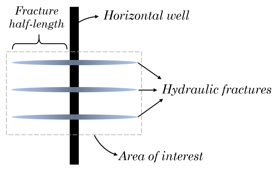
(b) Top view

Figure 2. A schematic of hydraulic fracturing design in horizontal wells

In the example presented in this section, the production from a horizontal well containing two parallel hydraulic fractures is modeled using different types of rocks. The aim is to show the effect of rock properties on the extent and severity of the pore pressure depletion and its subsequent effect on horizontal stresses, even by using the same boundary conditions.

A set of different rocks are examined by their response to pore pressure depletion. The problem assumptions are as follows. A horizontal well is drilled, and two parallel hydraulic fractures are created orthogonal to it. Both hydraulic fractures have reached their final length and effect of stress shadowing on their geometry during their propagation is neglected. Figure 3 shows the geometry of the problem for this example. The wellbore is put on continuous production for one month, one year, and five years. For handling production from fractures, total stress loading mode inside the fracture similar to Mathias et al (2010) is used. After each period of production, pore pressure, maximum horizontal stress ($\sigma_{H}$), minimum horizontal stress ($\sigma_{h}$), stress anisotropy ($\sigma_{H}-\sigma_{h}$) are calculated along an imaginary line (dashed red line in Figure 3) on the middle point between fractures. Moreover, the changes on these variables are going to be analyzed in two regions along that imaginary line. These two regions are Region 1 colored by yellow and Region 2 colored by green that respectively represent the area between two fractures and the zone in front of the fracture tips in Figure 3.

In this example, both hydraulic fractures are assumed to have the same lengths, and their half-lengths are equal to $30\;m$. Fracture spacing (orthogonal distance between fractures) also is equal to $30\;m$. Moreover, maximum horizontal stress, minimum horizontal stress, and reservoir pore pressure are assumed to be $56.53\;MPa$, $55.15\;MPa$, and $48.26\;MPa$ respectively. Furthermore, a constant pressure production is considered for the entire period of the production. Five different rocks are chosen for this purpose. The rocks have chosen somehow to represent a range of low-permeability reservoir rocks in terms of geomechanical properties, although in reality some of them are not reservoir rocks.

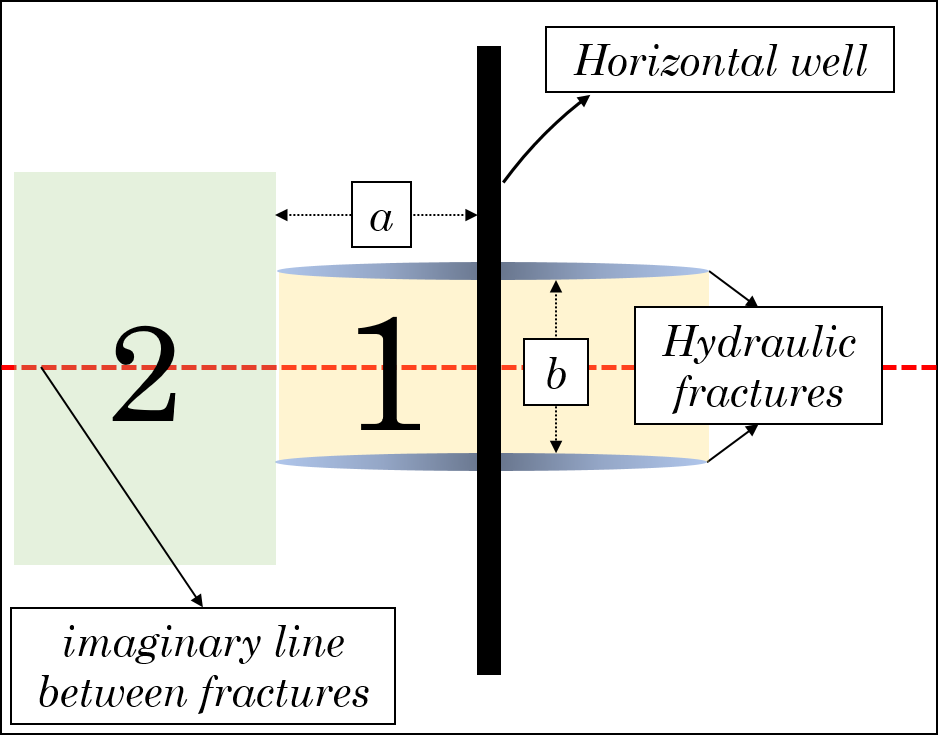
Figure 3. Geometry of the problem that is used for production

Table 1 presents the geomechanical properties of the rocks that are used for the analysis in this section. Relatively high permeability rocks (Weber Sandstone and Berea Sandstone) are placed deliberately in the analysis to show the difference in their pore pressure depletion compared to ultra tight rocks (Tennessee Marble, Charcoal Granite, and Haynesville Shale).

Table 1. Rock poroelastic properties used for the pore pressure depletion example. The table is constructed using Detournay et al (1989) and Rice and Cleary (1976). Haynesville shale properties are adopted from Chun (2013).

Rock type	$G,GPa$	$\nu$	$\nu_{u}$	$B$	$c,m^{2}/s$	$k,m^{2}$	$\alpha$
Tennessee Marble	$24$	$0.25$	$0.31$	$0.51$	$1.3\times 10^{-5}$	$1.0\times 10^{-19}$	$0.19$
Haynesville Shale	$13.8$	$0.22$	$0.46$	$0.91$	$4.5\times 10^{-6}$	$1.0\times 10^{-19}$	$0.96$
Berea Sandstone	$6$	$0.20$	$0.25$	$0.62$	$4.5\times 10^{-6}$	$1.9\times 10^{-13}$	$0.96$
Charcoal Granite	19	0.27	$0.30$	0.55	$7.0\times 10^{-6}$	$1.0\times 10^{-19}$	0.27
Weber Sandstone	12	0.15	0.29	0.73	$2.1\times 10^{-2}$	$1.0\times 10^{-15}$	0.64

Figure 4 shows pore pressure and stresses changes along the line of interest after one month of production. Figure 4a shows the pore pressure depletion along that line. Both sandstones experience more than $50\%$ reduction in the pore pressure in Region $1$. However, Charcoal Granite shows no change in the pore pressure in that region, Tennessee Marble experiences a slightly small depletion, and Haynesville shale shows a slight increase in pore pressure in the same region. Maximum horizontal stress shows the same trend as pore pressure, but minimum horizontal stress shows a reverse trend. Both sandstones have the highest reduction in the magnitudes of the maximum and minimum horizontal stresses and their stress anisotropies among the analyzed set. Tennessee Marble and Charcoal Granite show a small reduction in the magnitude of these parameters, but the Haynesville Shale behavior is slightly different from other rocks in Regions 1 and 2. A slight increase in observed in pore pressure and maximum horizontal stress of Haynesville Shale in Region 1, while its behavior falls in between two sandstones and ultra-tight rocks.

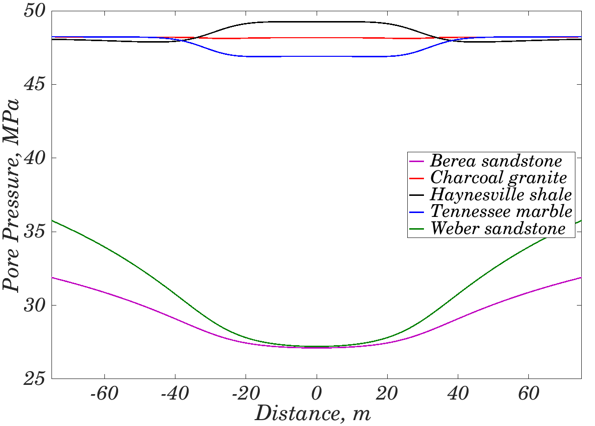
(a) Pore pressure

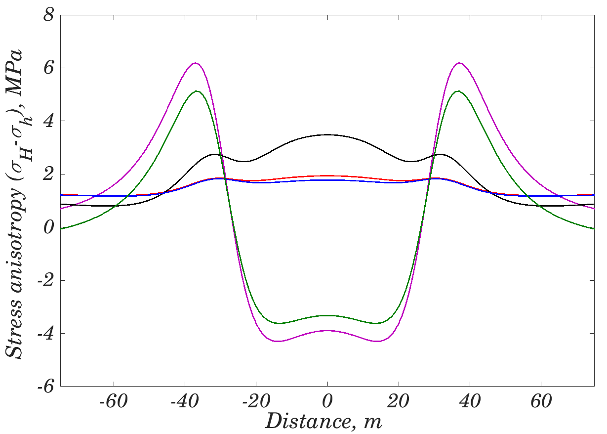
(b) Stress anisotropy

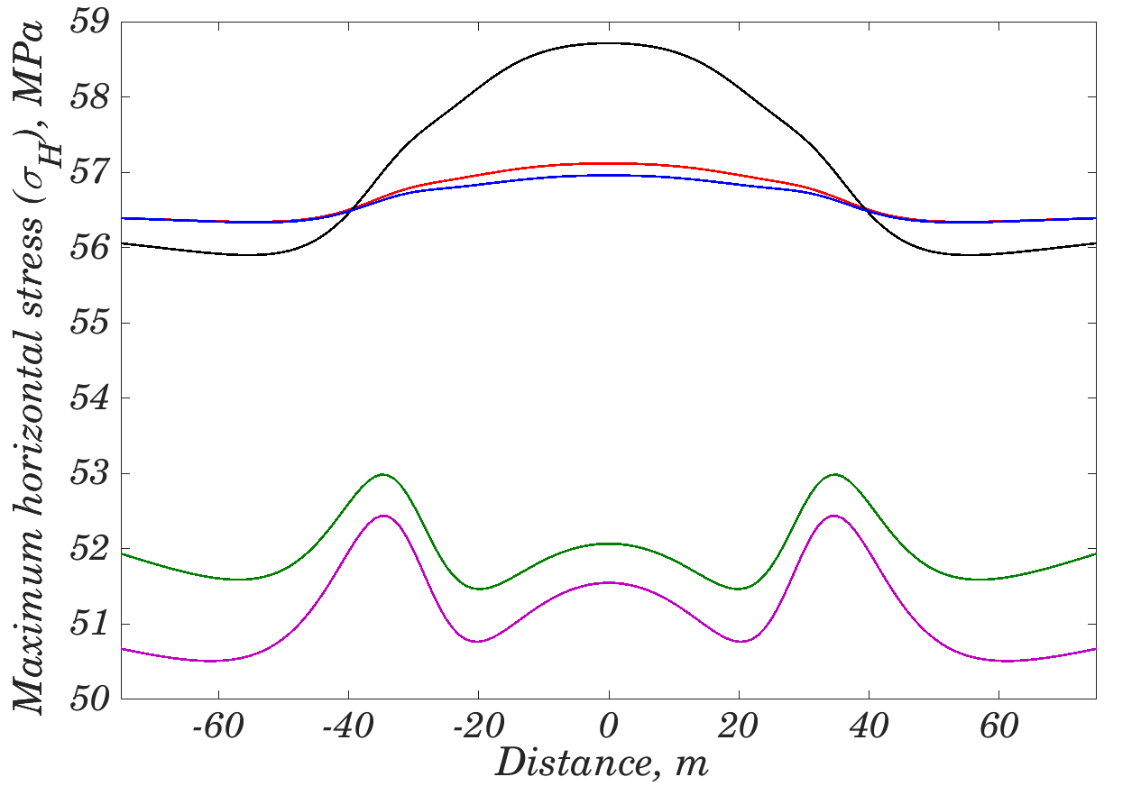
(c) $\sigma_{xx}$

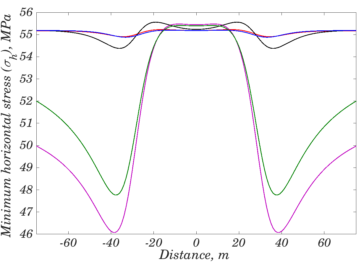
(d) $\sigma_{yy}$

Figure 4. Response of different rocks after $1$ month of production

Another calculation is done on the same line after $1$ year from production. Figure 5 shows changes of the variables along the interested line. After one year, pore pressure depletion in Region $1$ has reached to the pre-set value ($27\;MPa$) for both sandstones. Also, pore pressure reduction has traveled more in Region 2. The other three rock samples show partial depletion in Region 1. As is shown in Figure 5a pore pressure reduction of Haynesville Shale in Region 1 is highest among other rocks after one year. It is also observed that the shale shows a different behavior in terms of the magnitude of both horizontal stresses and anisotropy (Figure 5c and 5d) in both Regions. Moreover, the magnitude of these stresses is decreased and stays between a minimum that belongs to sandstones and a maximum that belongs to Charcoal Granite and Tennessee Marble. For the changes in stress anisotropy, after one year it is observed that the stress anisotropy for shale is slightly below of the original value ($1.38\;MPa$).

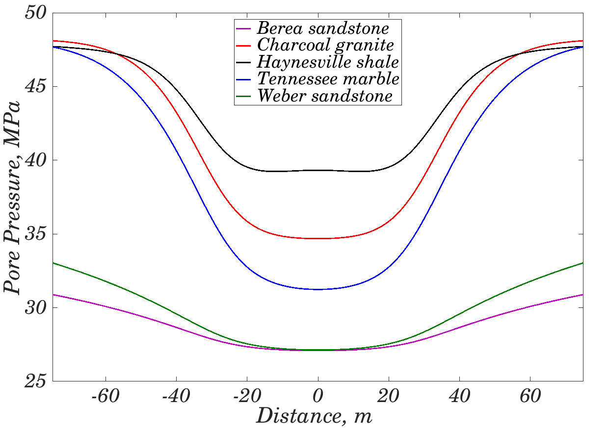
(a) Pore pressure

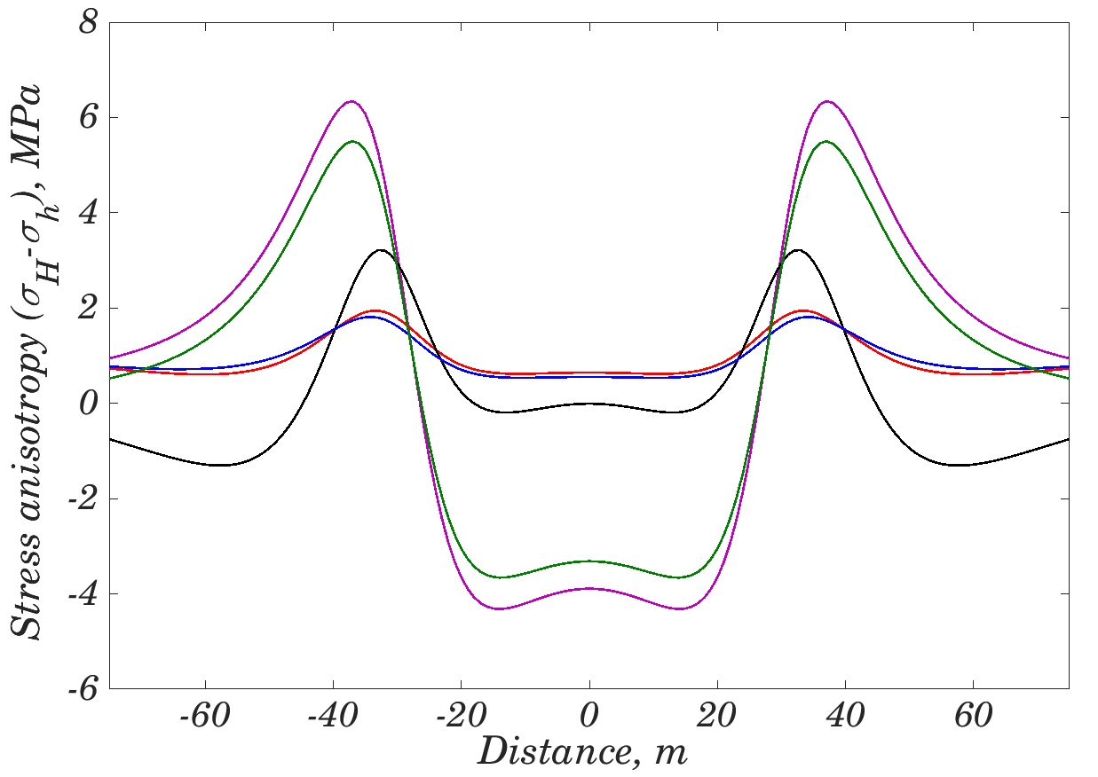
(b) Stress anisotropy

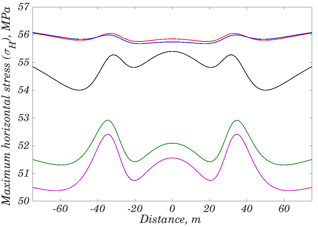
(c) $\sigma_{xx}$

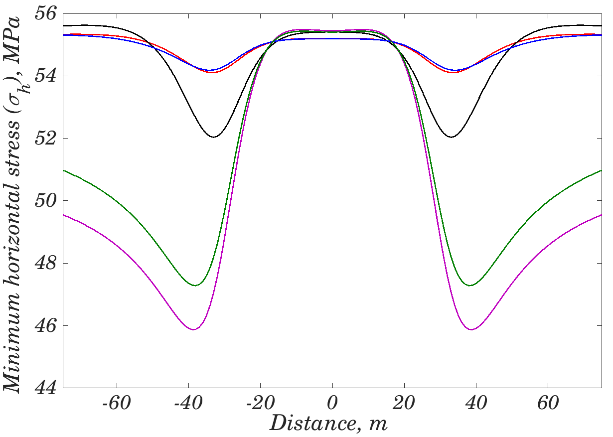
(d) $\sigma_{yy}$

Figure 5. Response of different rocks after $1$ year of production

Plots of the same calculations after five years are shown in Figure 6. At this time, pore pressure reduction of the Shale, Charcoal granite, and Tennessee Marble has not reached to the prescribed value yet (this happened in sandstones after one year of production). The pore pressure depletion of sandstones, unlike the other three types of rocks, has traveled in Region 2. Comparing pore pressure depletion of the three tight rocks shows that the shale has been depleted less than the other two in Region 1. Regarding stress, shale has decreased further down, and at this time its stress magnitudes are at the same level as sandstones. The stress anisotropy plot after five years also shows that stress reversal has happened for shale and two sandstones, although no change or slight change is observed in the other two tight rocks.

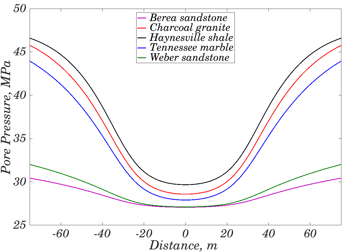
(a) Pore pressure

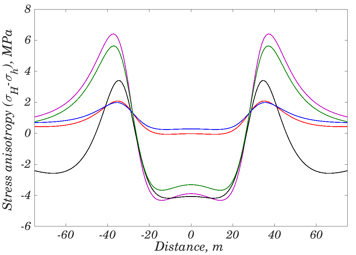
(b) Stress anisotropy

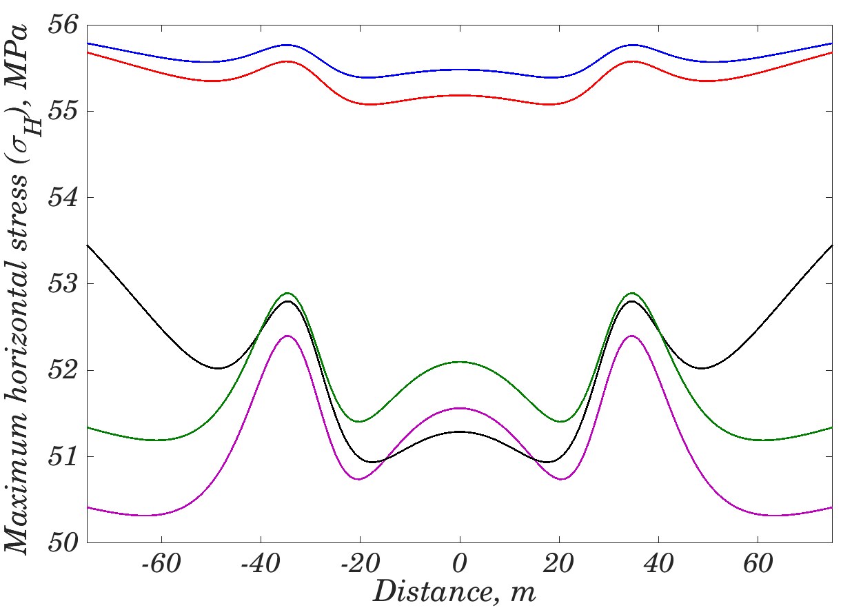
(c) $\sigma_{xx}$

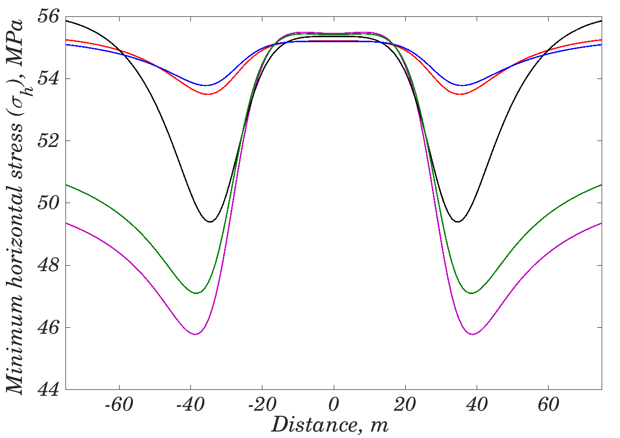
(d) $\sigma_{yy}$

Figure 6. Response of different rocks after $5$ years of production

The results of the analysis that was performed using different rock properties may be used to categorize the rock samples that were used in this section into three groups having different behaviors. Berea Sandstone and Weber Sandstone formed the first group. This group of rocks showed complete depletion in Region 1 as early as $1$ month from production. Pore pressure reduction for these two rocks also travels in more in Region 2 compared to the other three rocks. Haynesville Shale showed a different behavior compared to the other four rocks chosen for this study under the loading condition and problem geometry that was described. The pore pressure depletion plots show that the magnitude of the stresses in both of sandstones stay low as a result of depletion during the period of production, and so does their stresses. On the other hand, pore pressure depletion for Charcoal Granite and Tennessee Marble happens very slow, and their stress magnitudes stay the highest during the period that was discussed. At early time, shale showed a slight increase in the amount of pore pressure and stresses. Also, after one year its pore pressure was reduced less than any other rock sample in this study, its stress magnitude was less than Charcoal Granite and Tennessee Marble and higher than the sandstones. After five years of production, although the area between fractures has not been depleted entirely in shales, the stresses reach their minimum, as low as sandstones, and stress reversal happens.

4. GLOBAL SENSITIVITY ANALYSIS OF PORE PRESSURE AND STRESSES

In this section, Sobol method is used to analyze the variation of the model output parameters resulting from changes in the inputs. Pore pressure $p_{p}$, maximum horizontal $\sigma_{H}$, and minimum horizontal stress $\sigma_{h}$ are chosen as our quantities of interest (QI). We are precisely interested in tracking the changes of QI at six points around hydraulic fractures and horizontal well as the production time increases. Locations of these six points are shown in Figure 7. Among them, Points $4$ and $1$ are on the path of the infill (off-set) horizontal well and Points $2$, $3$, $5$, and $6$ are on the path of child fracture propagation in refracturing or infill well stimulation. We, intentionally, set the far-field stresses and pore pressure constant during production to limit our analysis to a single well. The prescribed values for these fixed boundary conditions are given in Table 2. To track the changes of QI with time, the model is set for three different production periods of $1\;month$, $1\;years$, and $3\;years$. For each of these cases, the simulator is run for a total of $10800$ times to generate the output vectors. Three vectors for pore pressure, maximum horizontal, and minimum horizontal stresses are generated at the end of each period of production.

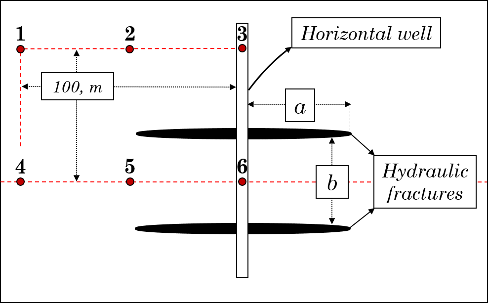
Figure 7. Locations of the six points that are chosen for calculating the changes in QI

Maximum horizontal stress, $\sigma_{H}$	$58.60\text{ MPa}$
Minimum horizontal stress, $\sigma_{h}$	$55.15\text{ MPa}$
Reservoir pore pressure, $p_{r}$	$48.26\text{ MPa}$

Table 2. Input parameters of for the reservoir far-field properties

We selected eight independent input variables for the global sensitivity analysis. The input variables are divided into two separate categories, namely the stimulation design variables and rock properties. Table 3 presents these variables and their minimum and maximum values. The design variables include fracture half-length $a$, fracture spacing $b$, and production pressure (fracture pressure) $p_{f}$. For all of the simulations, fracture pressure was held constant during the period of the production. Rock properties the were selected for sample generation include shear modulus $G$, undrained Poisson’s ratio $\nu_{u}$, drained Poisson’s ratio $\nu$, Skemtson’s coefficient $B$, and mobility $\kappa$ (rock absolute permeability $k$/fluid viscosity $\mu$).

Table 3. Rock poroelastic properties and design variables that are used global sensitivity analysis. The ranges of rock properties are chosen from Cheng (2016). Note that in this section and the following sections of the paper, $\log()$ of the fluid mobility is refereed to as $\kappa$.

	Design variables			Rock properties
Property	$a,\;m$	$b,\;m$	$p_{f},\;MPa$	$G,GPa$	$\nu_{u}$	$\nu$	$B$	$\log(\kappa),\frac{m^{2}}{Pa\cdot s}$
Minimum	$10$	$10$	$10$	$1$	$0.30$	$0.1$	$0.3$	$-17$
Maximum	$60$	$30$	$40$	$25$	$0.45$	$0.29$	$0.9$	$-10$
Sobol index	$S_{1}$	$S_{2}$	$S_{3}$	$S_{4}$	$S_{5}$	$S_{6}$	$S_{7}$	$S_{8}$

Referring to Equation (2.11), number of total terms for the analysis using $8$ input variables will be $2^{8}\;=256$, which is also equal to the total number of Sobol indices. Each of the variables in Table 3 are associated with a Sobol index as shown in the table. Using this convention, a first order Sobol index $S_{i}$ is related to individual contributions of the variables on the output, while higher order Sobol indices $S_{i\dots j}$ represent the interaction between the variables. For example, $S_{1}$ represents the effect of changes in fracture half-length magnitude to the variation of a specific output variable (e.g., pore pressure), and $S_{37}$ represents this variation due to the simultaneous changes in fracture pressure $p_{f}$ and Skemptson’s coefficient $B$. Using this procedure, three output vectors for pore pressure, maximum stress, and minimum stress are generated for each period, and each of these vectors is analyzed. An open-source library developed by Herman and Usher (2017) for sensitivity analysis is used to perform both the sample generation and Sobol analysis. Results are discussed in the next section.

4.1. Analysis of the results after one month

In this section, a global sensitivity of the pore pressure and stresses after $1\;month$ of production is presented. After one month, it not expected from pore pressure depletion extent to move far away from the wellbore. Figures 8–10 show the result of SA for this production period. As presented in Figure 8a for pore pressure, the main individual contributions to changes of the pore pressure are $S_{8}$ and $S_{3}$, which correspond to mobility $\kappa$ and production pressure $p_{f}$ respectively. These two variables contribute to more than $80\%$ of the changes in pore pressure changes around hydraulic fractures and horizontal well. Also, an interesting observation is that $S_{1}$ (fracture half-length) contributes to $10\%$ of the changes at Point $5$. This is important because Point $5$ is the desired path for propagation of the child fracture in refracturing process. Figure 8b shows the interaction effects $S_{ij}$ between the selected input parameters. Any Sobol index that has a value less than $0.01$ is excluded. This does not put any limitation on our analysis since $\Sigma S_{i\dots j}\approx 0.85-0.9$ at each point. As expected, the interaction between production pressure and mobility have the greatest contribution among other interactions. Also, a small contribution is observed from $S_{48}$ at Points $1$, $2$, $3$, and $6$.

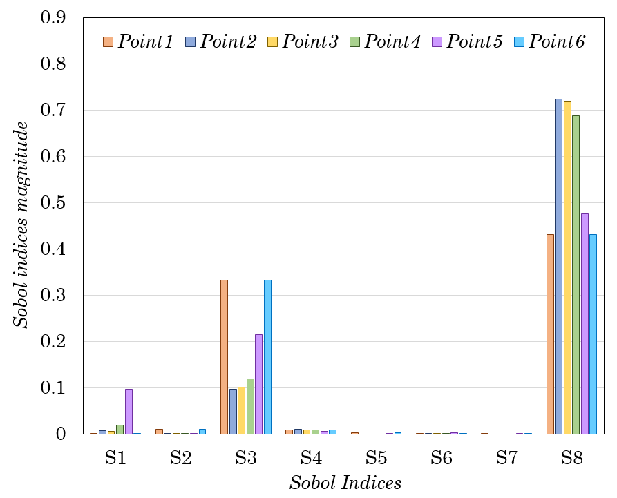
(a) Individual effects

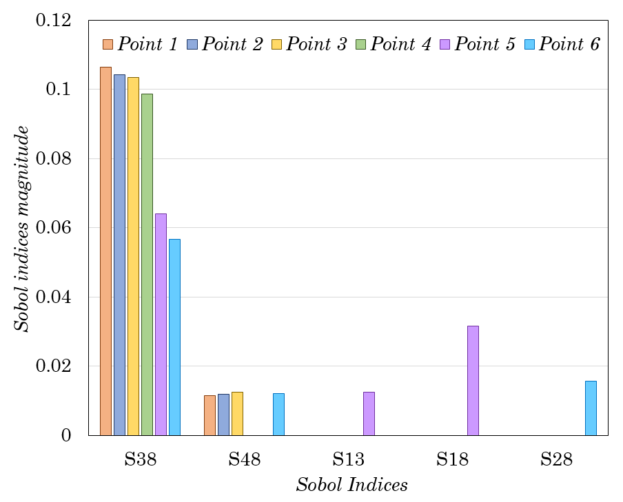
(b) Interaction effects ($>0.01$)

Figure 8. Sobol indices of the input sample for pore pressure after 1 month from production

Figure 9a shows the individual contributions of inputs on the minimum horizontal stress. It is observed that $B$, $p_{f}$, and drained Poisson’s ratio $\nu$ are the main contributors to the changes of the minimum horizontal stress at the points that are located outside the fracture spacing (i.e., Points $1$, $2$, $3$, and $4$) in this case. However, for the points close to the fracture tip area, and inside the spacing (i.e., Points $5$ and $6$), different results are observed. At Point $5$, fracture half-length $a$ and $B$ are significant contributors, while at Point $6$ fracture half-length $a$ and fracture spacing $b$ are the dominating contributors among other individual terms. Also, it is observed that changes of fracture half-length and fracture spacing ($S_{12}$) have the most significant impact ($\approx\;24\%$) on the minimum horizontal stress at Point $6$, compared to all other variables. This shows the importance of these two variables on the minimum horizontal stress changes. Note that Point $6$ is the possible path of child fracture initiation in refracturing. At the points outside the fracture spacing area, however, $S_{38}$, $S_{68}$, and $S_{78}$ have the main contributions to changes of minimum horizontal stress.

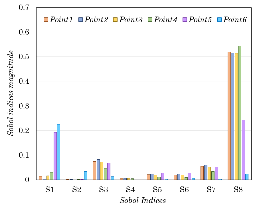
(a) Individual effects

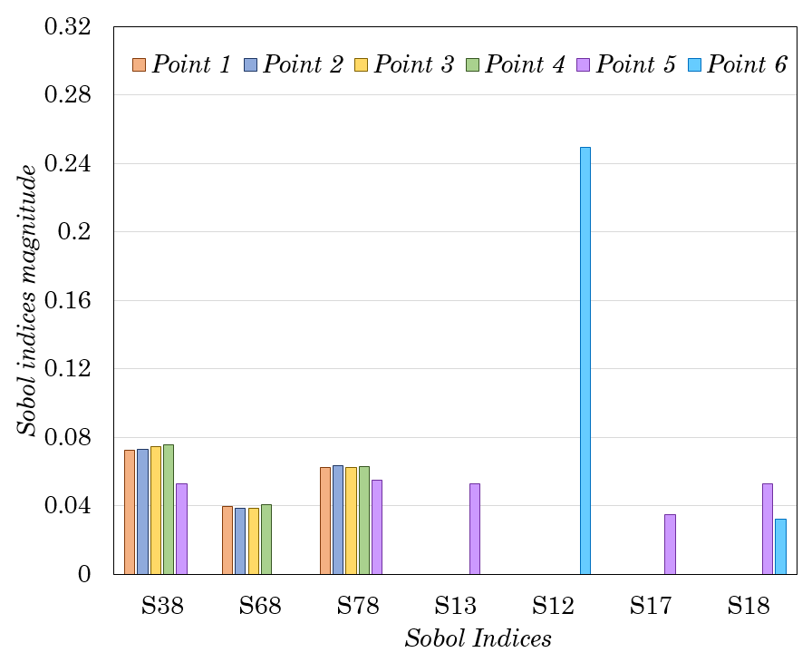
(b) Interaction effects ($>0.03$)

Figure 9. Sobol indices of the input sample for minimum horizontal stress after 1 month from production

Figure 10a shows the first order Sobol indices $S_{i}$ for maximum horizontal stress. In this case, main contributions are $S_{8}$, $S_{3}$, $S_{7}$, $S_{6}$, and $S_{5}$ respectively. No significant contribution from design variables $a$ and $b$ is observed. Also, The main effect for interaction terms are due to $S_{38}$, $S_{78}$, $S_{68}$. From this, it can be concluded that the main contributions to the changes in maximum horizontal stress are due to the rock properties rather than the design variables. These variables contribute to about $70\%$ of the changes in maximum horizontal stress. It should be noted that although $p_{f}$ is among design variables, the main source of the changes due to this variable is the difference between this variable and far-field pore pressure ($\Delta p$).

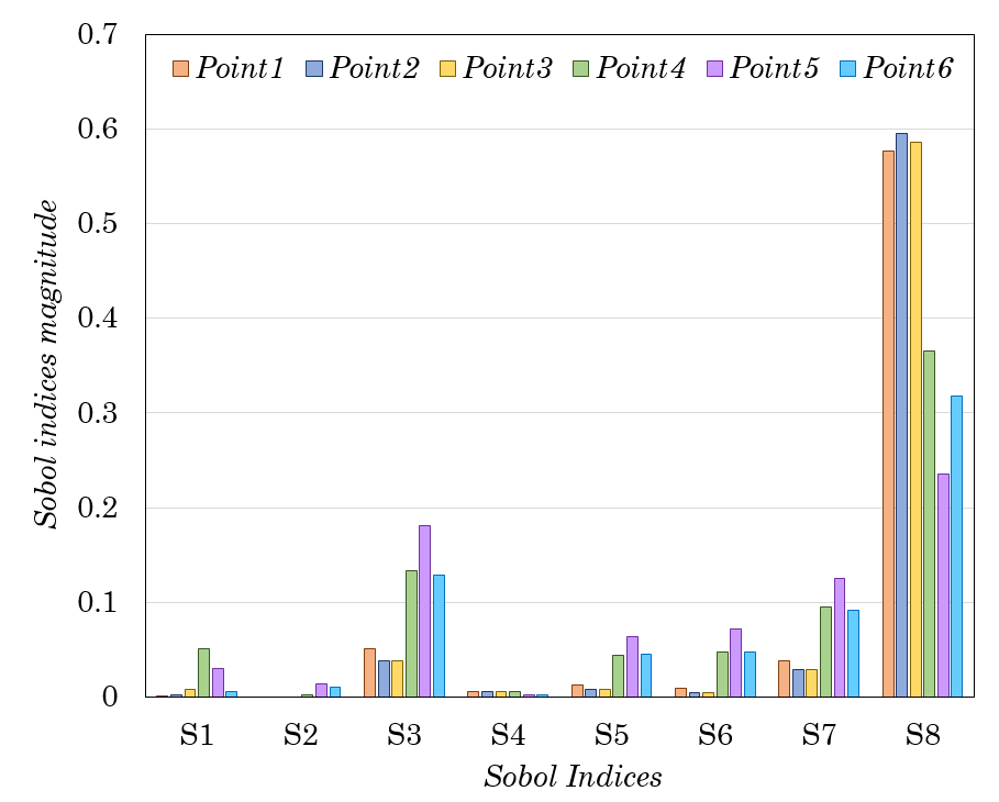
(a) Individual effects

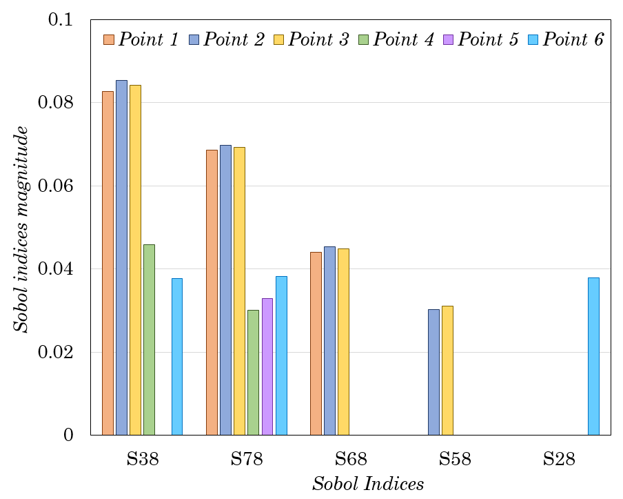
(b) Interaction effects ($>0.03$)

Figure 10. Sobol indices of the input sample for maximum horizontal stress after 1 month from production

4.2. Analysis of the results after one year

Figures 11–13 show the results of Sobol analysis after one year from production. There are some similarities and several differences in the dominant contributors compared to the results after $1\;month$. For example, similar to the $1$ month case, $S_{3}$ and $S_{8}$ are still dominating individual contributors to the variance of the pore pressure as shown in Figure 11a. In contrary, unlike the $1\;month$ case, the effect of $S_{3}$ is greater than $S_{8}$ at Point $6$ after $1\;year$. The main reason for this is that the effect of pore pressure depletion has reached to the half-way between fractures after this period. Among higher order Sobol indices, $S_{38}$ has the greatest impact on the pore pressure changes. The second greatest impact from interaction terms is due to $S_{18}$, while after a month $S_{48}$ was the second dominant contributor among higher-order indices.

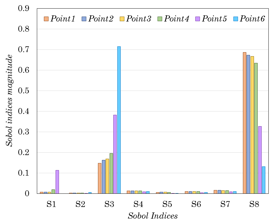
(a) Individual effects

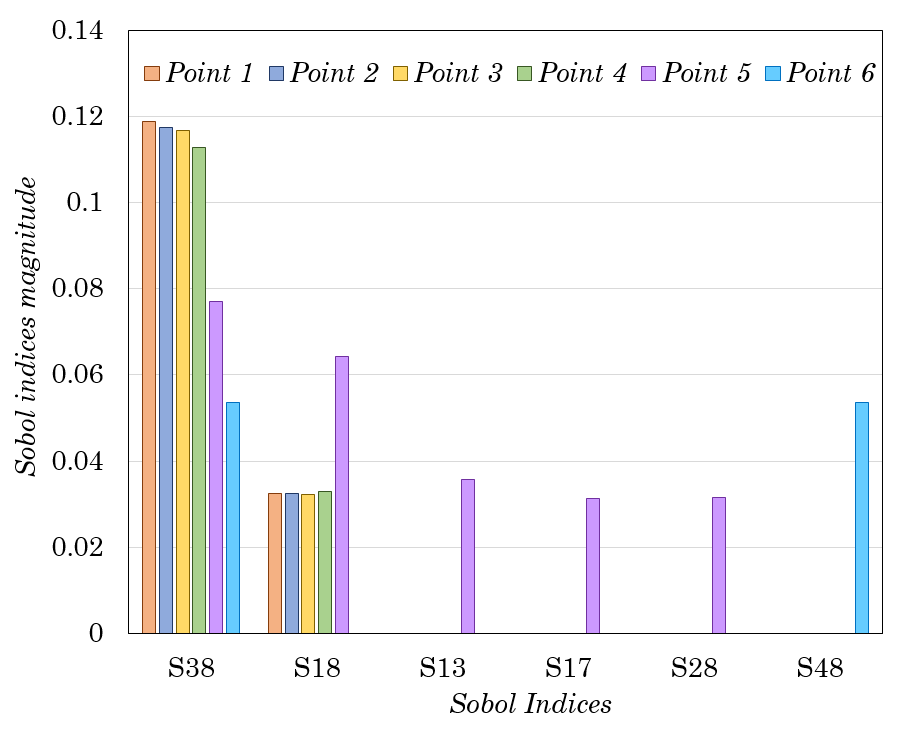
(b) Interaction effects ($>0.03$)

Figure 11. Sobol indices of the input sample for pore pressure after 1 year from production

Sobol indices for minimum horizontal stress are presented in Figure 12. The dominant individual Sobol indices are the same as $1\;month$ in this case. The only difference is that all of the rock properties variables have a more significant Sobol index after one year, indicating advancement of the pore pressure depletion in the rock. Among interaction terms, $S_{38}$ and $S_{78}$ are the dominating interactions. Unlike the $1\;month$ case, there is no significant impact from $S_{68}$. Also, $S_{12}$ is still the greatest Sobol index at Point $6$, but its value has increased from $24\%$ to $40\%$.

Moreover, the combination of the fracture length and rock properties have a considerable impact on the changes in minimum horizontal stress at Point $5$. This makes sense because this point is in front of the fracture tip. The total contribution of the individual and interaction terms that include fracture length on the variance of minimum horizontal stress changes at Point $5$ is almost $65\%$.

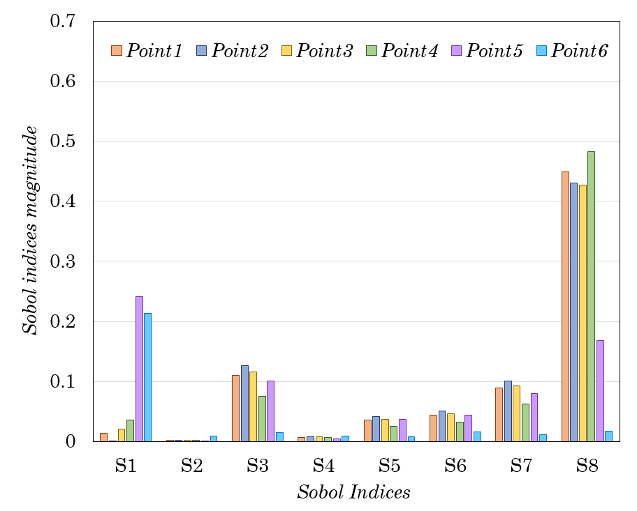
(a) Individual effects

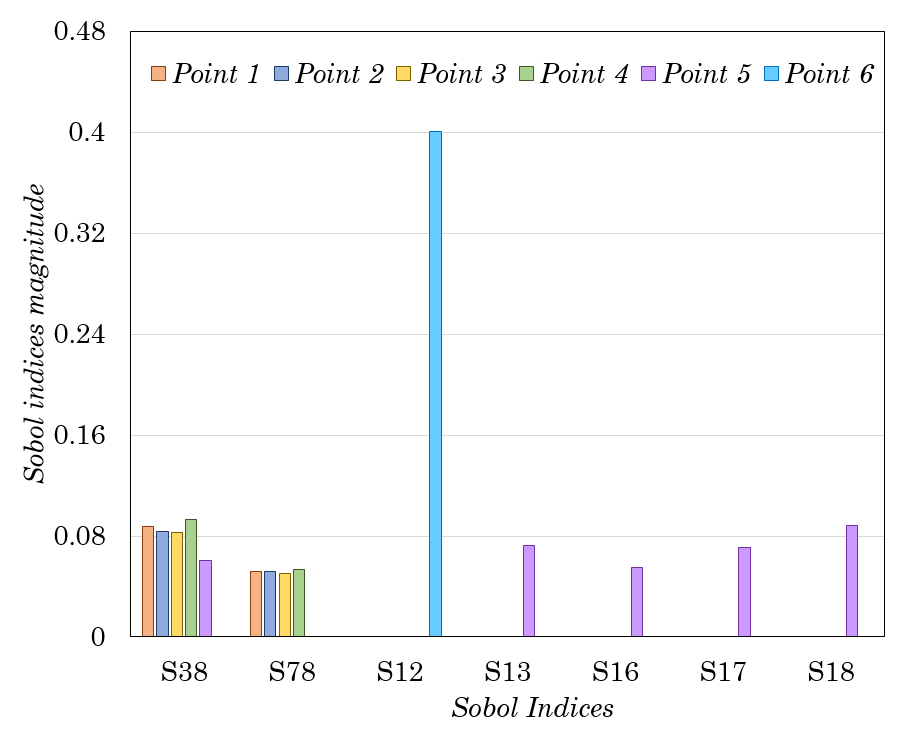
(b) Interaction effects ($>0.03$)

Figure 12. Sobol indices of the input sample for minimum horizontal stress after 1 year from production

Figure 13 represents the Sobol indices for maximum horizontal stress after one year. It can be seen that after one year, mobility has a smaller effect on the changes in maximum horizontal stress compared to the one month case. But, the contribution from $S_{3}$, $S_{5}$, $S_{6}$, and $S_{7}$ have increased. It is also observed that $S_{3}$ and $S_{7}$ are the dominant Sobol indices after one year. Among higher-order indices, $S_{17}$, $S_{18}$, and $S_{3}7$ are the dominant terms. Also, other terms such as $S_{38}$, $S_{48}$, $S_{58}$, $S_{68}$, $S_{78}$, and $S_{28}$ have considerable effects, but they do not affect all of the points equally

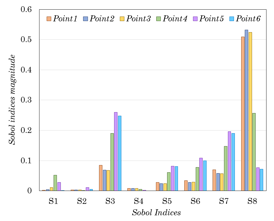
(a) Individual effects

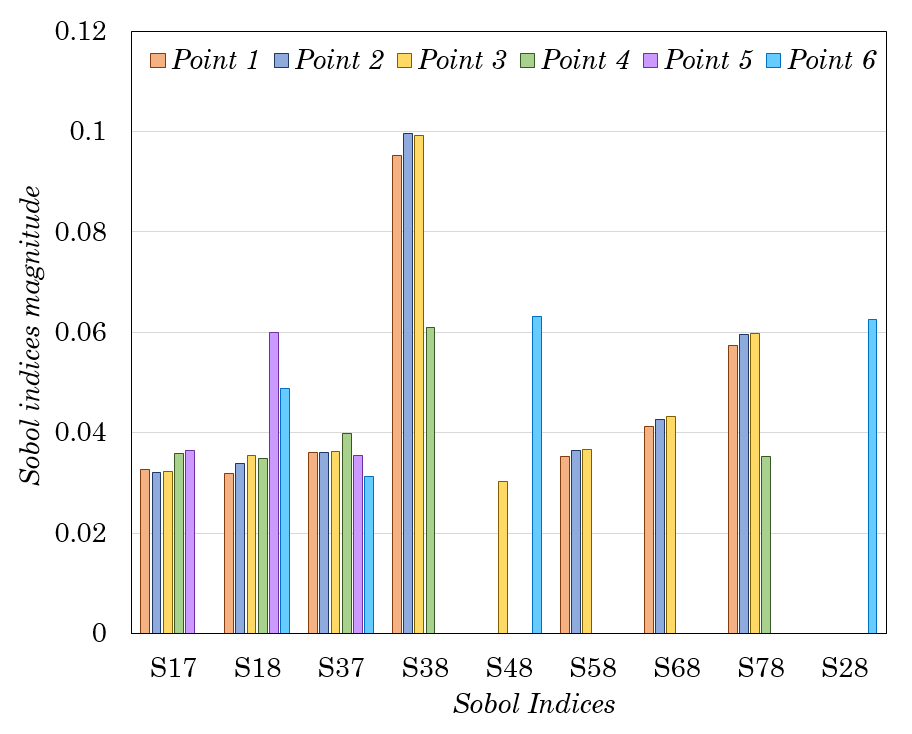
(b) Interaction effects ($>0.03$)

Figure 13. Sobol indices of the input sample for maximum horizontal stress after 1 year from production

4.3. Analysis of the results after three years

A similar analysis is performed after three years of production. Results are presented in Figures 14–16. Analysis of pore pressure (Figure 14) shows that as time progresses, $S_{8}$ decreases at all of the points. In contrary, $S_{3}$ increases as time progresses. The increase of $S_{3}$ at Points $5$ and $6$ is much more than the other points since they are closer to the spacing area between fractures. At Point $6$, almost $90\%$ of the variation in pore pressure is due to the changes in production pressure $p_{f}$, while this value is close to $50\%$ at Point $5$ and less than $30\%$ in the rest of points. Also, fracture half-length plays an important role in the variation of the pore pressure in the neighborhood of the tip region (Point $5$). The contribution of fracture half-length and its interactions with other terms on the variation of pore pressure at this point is close to $20\%$.

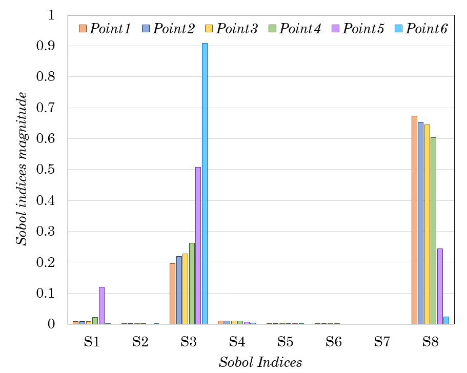
(a) Individual effects

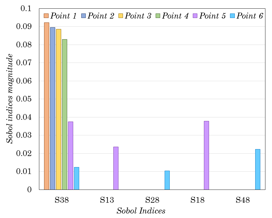
(b) Interaction effects ($>0.03$)

Figure 14. Sobol indices of the input sample for pore pressure after 3 years from production

Figure 15 represents the Sobol indices for minimum horizontal stress after three years. After this period, a slight decrease in $S_{8}$ is observed, while other individual indices stay almost constant. Two Points $5$ and $6$ are of particular interest for minimum horizontal stress. The dominant variable that causes most of the variation in minimum horizontal stress at these two points is fracture half-length. Also, $S_{12}$ contributes to about $45\%$ of the changes at Point $6$. Among interaction terms, $S_{38}$ and $S_{78}$ are the dominant interaction indices at all point except Point $6$, and $S_{12}$ at Point $6$ increases slightly compared to the case of $1\;year$.

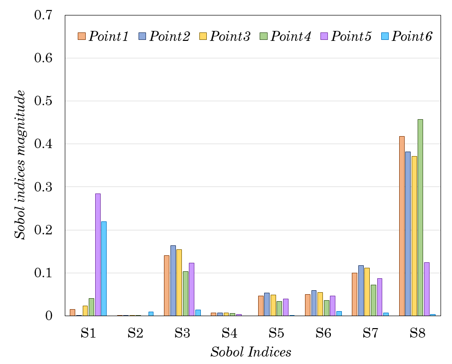
(a) Individual effects

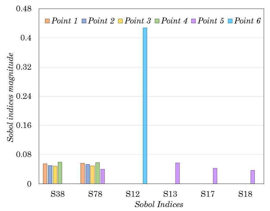
(b) Interaction effects ($>0.03$)

Figure 15. Sobol indices of the input sample for minimum horizontal stress after 3 years from production

Figure 16 presents the Sobol analysis results for maximum horizontal stress after $3\;years$. Similar to changes that were observed by comparing $1\;year$ and $1\;month$ results, it is observed in this case that the effect of $S_{8}$ decreases further compared to $1\;year$. However, the rate of changes is less than the changes that were observed between two previous changes. Also, it observed that $S_{3}$ increases at all of the points. Moreover, the dominant interaction indices that are greater than $0.03$ have decreased from nine to four.

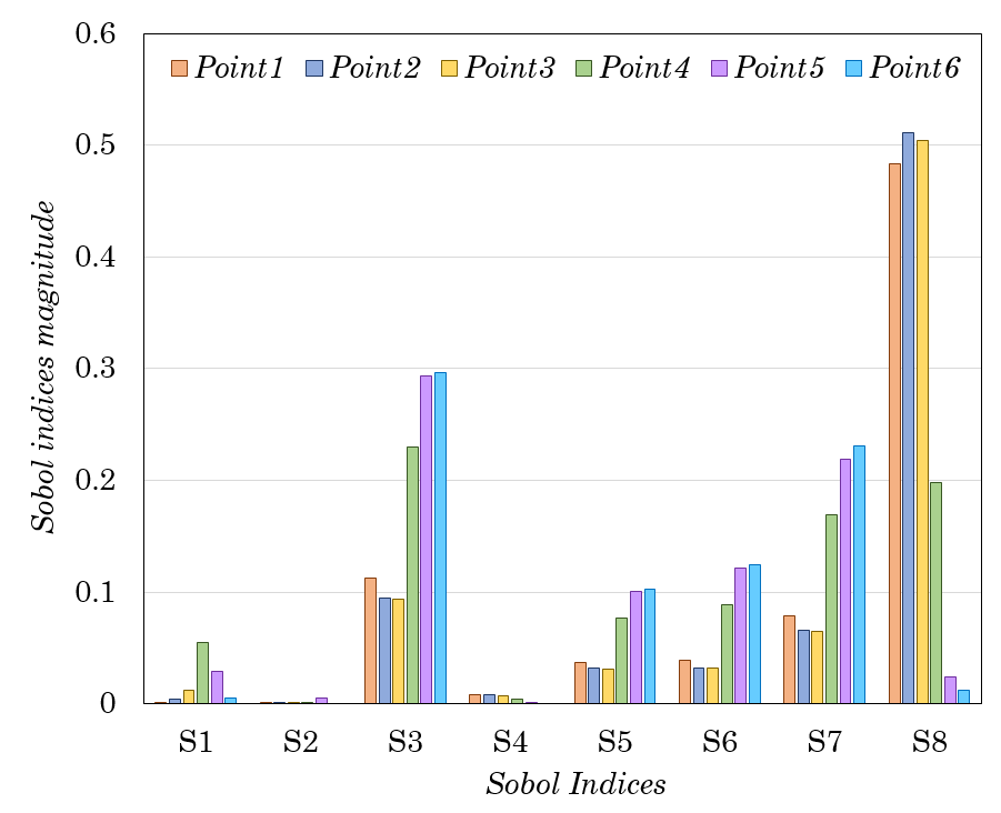
(a) Individual effects

(b) Interaction effects ($>0.03$)

Figure 16. Sobol indices of the input sample for maximum horizontal stress after 3 years from production

5. REDUCED ORDER MODEL FOR PORE PRESSURE AND STRESSES

In this section, we utilize one of the greatest benefits of the Sobol analysis which is its ability to present a reduced order (mathematically simple) model (ROM) for a relatively complex function such as the one that we discussed in Section 2.2. For this purpose, we consider the case of production from the hydraulically-fractured well for one year (Section 4.2) and present a ROM for for pore pressure, maximum horizontal stress, and minimum horizontal stress at different points around fractures. In our approach, we use those Sobol indices that contribute to $80\%$ to $90\%$ changes in the results.

In order to be avoid repetition, we group the points at which pore pressure and stresses reduces similarly. It was observed that the points located outside the spacing area (i.e., Points 1 - 4) show the same behavior in terms of the dominant Sobol indices, and, correspondingly, their corresponding dominant Sobol functions are similar. Therefore, as a representative of these points we only present the reduced order model for Point 1. Next, we present the ROM for Points 5 and 6 because these two pints showed different behavior, and their representative Sobol functions are different.

5.1. Sobol functions and ROM at Point 1

Pore pressure.

As shown in Figure 11, production pressure $P_{p}$, mobility $\kappa$, and their combinations (i.e., $S_{3},\;S_{8},\;S_{38}$) accounts for more than $90\%$ of the pore pressure changes at Points 1–4. Therefore, a reduced order model (ROM) may be presented using these variables at these points. For example, Equation (2.11) for pore pressure at Point 1 with $90\%$ accuracy may be written as:

$$Pp^{p_{1}}_{1year}=f_{0}+f_{3}+f_{8}+f_{38}$$ (5.1)

Figure 17 shows these three functions correspondingly. It can be seen that the pore pressure is directly related to production pressure $p_{f}$. It is also has an inverse relationship with $\log()$ of the fluid mobility. As shown in Figure 17b, extremely low fluid mobilities (i.e., $>10^{-13}\;\frac{m^{2}}{Pa.s}$), the function is almost constant and changes in fluid mobility will not affect the pore pressure.

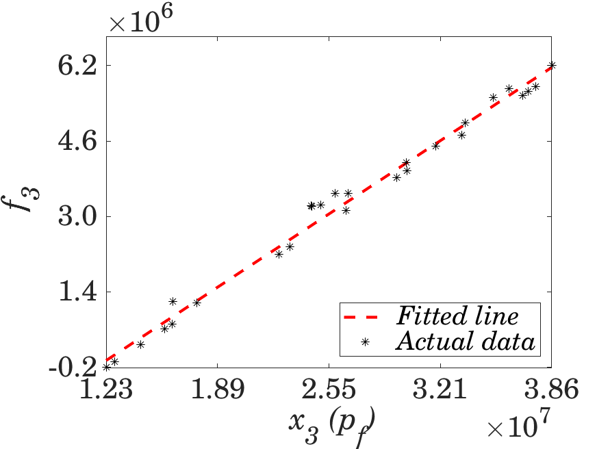
(a) $f_{3}$

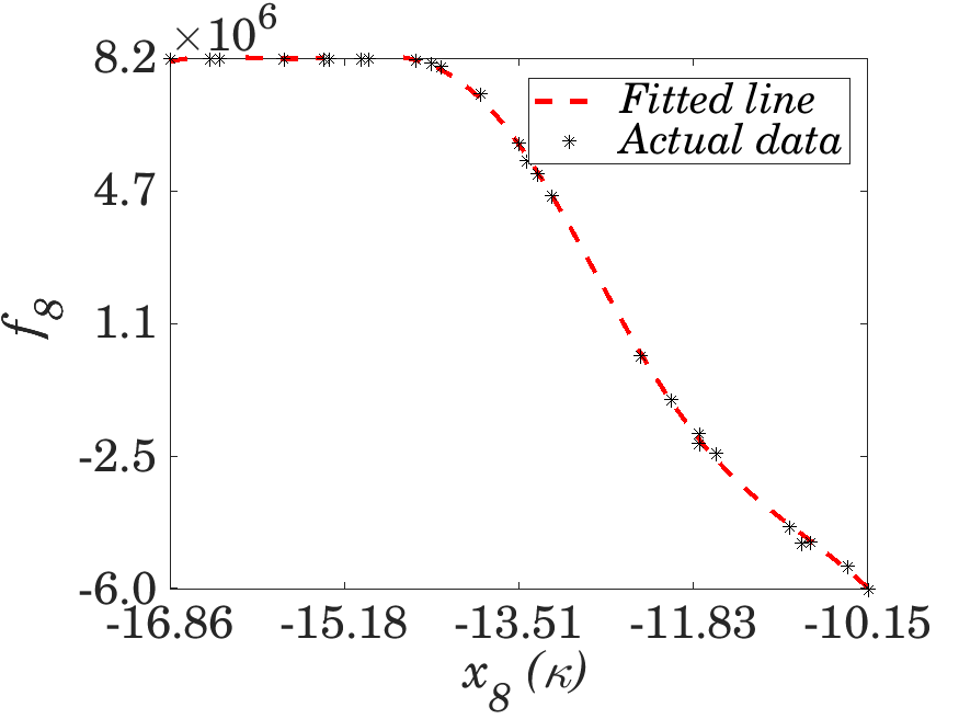
(b) $f8$

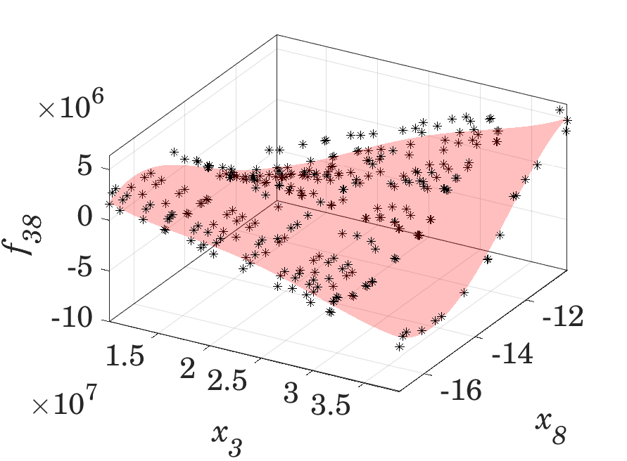
(c) $f_{38}$

Figure 17. The dominant Sobol functions for pore pressure at Point 1.

Using Equation (5.1) and Figure 17 one may construct the reduced order model with the following items:

$$f_{0}= \;A_{0}$$ (5.2a)

$$f_{3}= \;A_{0}\;p_{f}+A_{1}$$ (5.2b)

$$f_{8}= \;A_{0}\;\sin(A_{1}\;\kappa+A_{2})+A_{3}\;\sin(A_{4}\;\kappa-A_{5})$$ (5.2c)

$$f_{38}= -A_{0}-A_{1}\;p_{f}-A_{2}\;\kappa-A_{3}\;p_{f}^{2}+A_{4}\;p_{f}\;\kappa+A_{5}\;\kappa^{2}+A_{6}\;p_{f}^{3}-A_{7}\;p_{f}^{2}\;\kappa-A_{8}\;p_{f}\;\kappa^{2}-A_{9}\;\kappa^{3}$$ (5.2d)

where the coefficients for each function is presented in Table 4 in the Appendix.

Minimum horizontal stress.

Similar analysis can be done for minimum horizontal stress at Point 1. As shown in Figure 12, the dominant Sobol indices for minimum horizontal stress at Point 1 are $S_{3}$, $S_{5}$, $S_{6}$, $S_{7}$, $S_{8}$, $S_{38}$, and $S_{78}$. Figure 18 shows th plots of these variables and their corresponding Sobol function for minimum horizontal stress after one year from production. It can be observed that pore pressure, drained Poisson’s ratio, and Skemptson’s coefficient have a directly effect on the minimum horizontal stress, and undrained Poisson’s ratio and mobility have an inverse effect on the minimum horizontal stress at Point 1.

(a) $f_{3}$

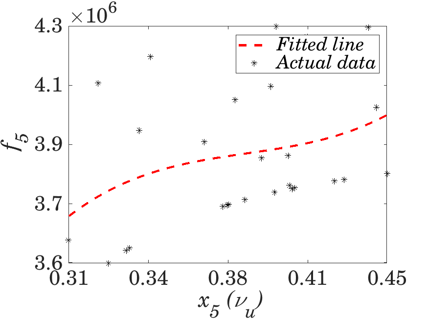
(b) $f_{5}$

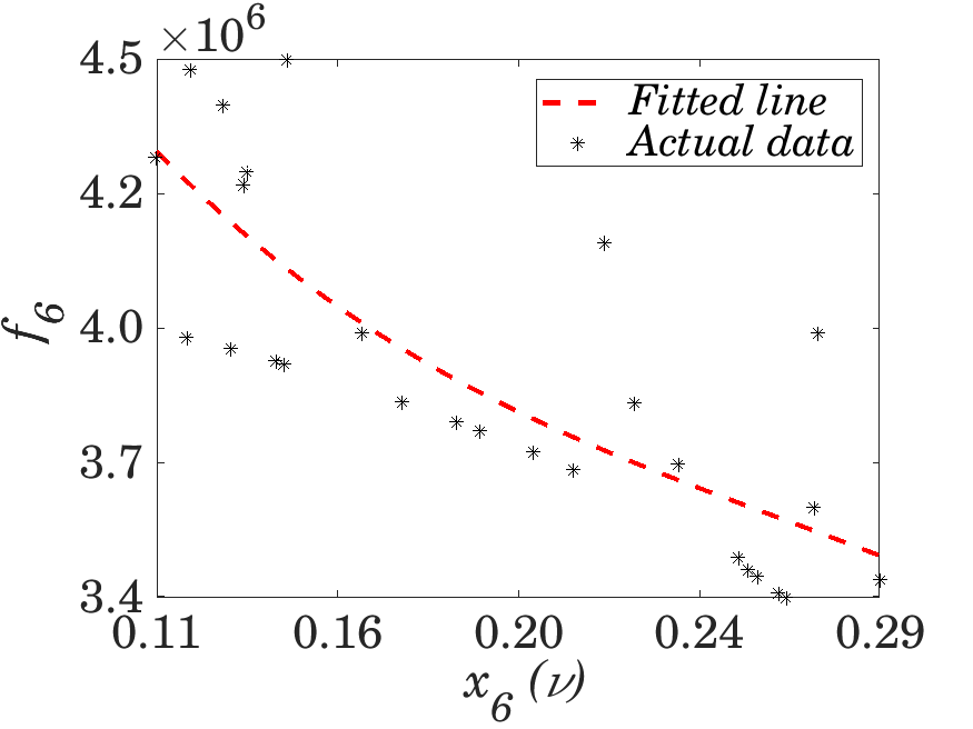
(c) $f_{6}$

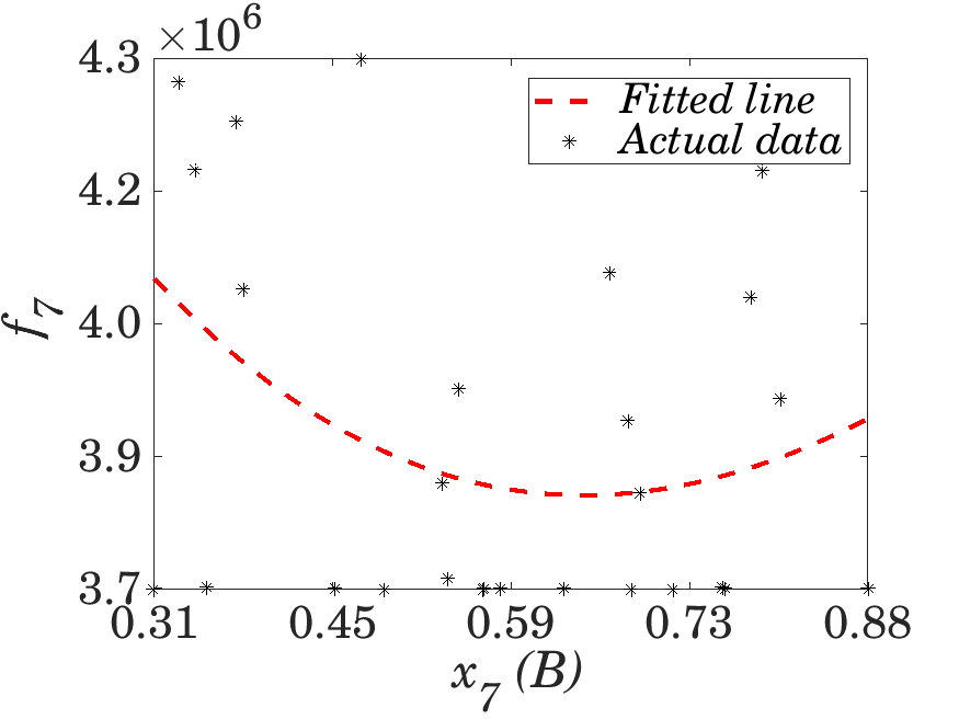
(d) $f_{7}$

(e) $f_{8}$

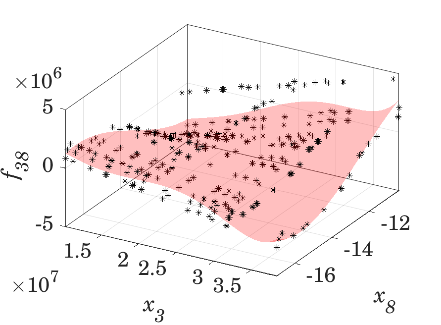
(f) $f_{38}$

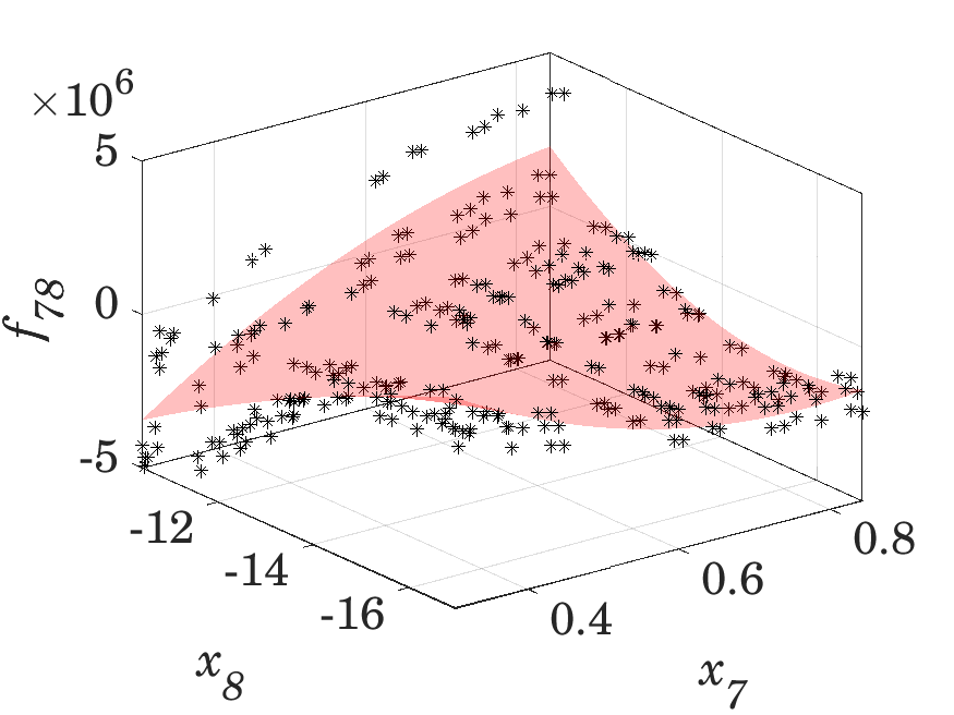
(g) $f_{78}$

Figure 18. The dominant Sobol functions for minimum horizontal stress at Point 1.

For the minimum horizontal stress at Point 1, the following reduced order function may be constructed:

$$f_{0}= \;A_{0}$$ (5.3a)

$$f_{3}= \;A_{0}\;p_{p}+A_{1}$$ (5.3b)

$$f_{5}= \;A_{0}\;\nu_{u}+A_{1}$$ (5.3c)

$$f_{6}= \;A_{0}\;\nu-A_{1}$$ (5.3d)

$$f_{7}= \;A_{0}\;B^{3}-A_{1}\;B^{2}+A_{2}\;B-A_{3}$$ (5.3e)

$$f_{8}= \;A_{0}\;\sin(A_{1}\;\kappa+A_{2})+A_{3}\;\sin(A_{4}\;\kappa-A_{5})+A_{6}\;\sin(A_{7}\;\kappa+A_{8})$$ (5.3f)

$$f_{38}= \;-A_{0}+A_{1}\;p_{f}-A_{2}\;\kappa-A_{3}\;p_{f}^{2}-A_{4}\;p_{f}\;\kappa+A_{5}\;\kappa^{2}-A_{6}\;p_{f}^{3}+A_{7}\;p_{f}^{2}\;\kappa-A_{8}\;p_{f}\;\kappa^{2}+A_{9}\;\kappa^{3}$$ (5.3g)

Coefficients of the functions in Equations (5.3a)–(5.3g) are presented in Table 5.

Maximum horizontal stress.

It can be verified that $f_{3}$, $f_{5}$, $f_{6}$, $f_{7}$, $f_{8}$, and $f_{38}$ are the dominant Sobol indices that affect the maximum horizontal stress at Point 6. As shown in Figure 13, these variables generate about $90\%$ of the calculated model’s maximum horizontal stress. Therefore, one may construct the ROM using these terms as:

$$\bar{\sigma}_{H_{1year}}^{P_{1}}=f_{0}+f_{3}+f_{5}+f_{6}+f_{7}+f_{8}+f_{38}$$ (5.4)

The corresponding Sobol functions for maximum horizontal stress are plotted in Figure 19. It was observed that $p_{f}$ and $\kappa$ show the same linear relationship with the reduced order function as in pore pressure and minimum horizontal stress. Also, similar to minimum horizontal stress, undrained Poisson’s ratio and mobility have effect on the minimum horizontal stress at Point 1.

(a) $f_{3}$

(b) $f_{5}$

(c) $f_{6}$

(d) $f_{7}$

(e) $f_{8}$

(f) $f_{38}$

Figure 19. The dominant Sobol functions for maximum horizontal stress at Point 1

For maximum horizontal stress, the ROM can be represented as:

$$f_{0}= \;A_{0}$$ (5.5a)

$$f_{3}= \;A_{0}\;p_{f}-A_{1}$$ (5.5b)

$$f_{5}= \;-A_{0}\;\nu_{u}+A_{1}$$ (5.5c)

$$f_{6}= \;A_{0}\;\nu^{2}-A_{1}\;\nu+A_{2}$$ (5.5d)

$$f_{7}= \;A_{0}\;B^{3}-A_{1}\;B^{2}+A_{2}\;B-A_{3}$$ (5.5e)

$$f_{8}= \;A_{0}\;\sin(A_{1}\;\kappa+A_{2})+A_{3}\;\sin(A_{4}\;\kappa-A_{5})+A_{6}\;\sin(A_{7}\;\kappa+A_{8})$$ (5.5f)

$$f_{38}= \;-A_{0}+A_{1}\;p_{f}-A_{2}\;\kappa+A_{3}\;p_{f}\;\kappa-A_{4}\;\kappa^{2}+A_{5}\;\kappa^{3}$$ (5.5g)

Coefficients of the function in Equations (5.5a)–(5.5g) are presented in Table 6. Similar analysis may be done for other points that are located at the outside of the spacing area. Also, it should be mentioned that the choice of the individual function in the reduced order model is arbitrary and by the best possible match. In the next section, Sobol functions and reduced order models for Point 5 is presented.

5.2. Sobol functions and ROM at Point 5

Pore pressure.

Point 5 is located at the point between the tips of the pre-existing fractures. Therefore, understanding the changes in pore pressure, the maximum and minimum horizontal stress at this point are extremely important for refracturing and infill drilling applications. The dominant variables affecting the pore pressure at Point 5 are fracture half-length ($a$), production pressure ($p_{f}$), mobility ($\kappa$) and the interaction between production pressure and mobility (cf., Figure 8). Figure 20 shows the plot of the corresponding Sobol functions for these variables.

(a) $f_{1}$

(b) $f_{3}$

(c) $f_{8}$

(d) $f_{38}$

Figure 20. Dominant Sobol functions for pore pressure at Point 5

As it can be seen, fracture half-length has a considerable effect on the pore pressure at Point 5. Change of fracture half-length (with the same spacing) from $57\;m$ to $10\;m$ will cause a reduction of $11\;Mpa$ in the pore pressure at Point 5. Using the fitted functions in Figure 20, the ROM for pore pressure at Point 5 after a year from production can be constructed as follows:

$$f_{0}= \;A_{0}$$ (5.6a)

$$f_{1}= \;-A_{0}\;a^{2}-A_{1}\;a+A_{2}$$ (5.6b)

$$f_{3}= \;A_{0}\;p_{f}-A_{1}$$ (5.6c)

$$f_{8}= \;A_{0}\;\sin(A_{1}\;\kappa-A_{2})+A_{3}\;\sin(A_{4}\;\kappa-A_{5})+A_{6}\;\sin(A_{7}\;\kappa+A_{8})$$ (5.6d)

$$f_{38}= \;-A_{0}+A_{1}\;p_{f}-A_{2}\;\kappa-A_{3}\;p_{f}^{2}+A_{4}\;p_{f}\;\kappa+A_{5}\;\kappa^{2}+A_{6}\;p_{f}^{3}-A_{7}\;p_{f}^{2}\;\kappa-A_{8}\;p_{f}\;\kappa^{2}+A_{9}\;\kappa^{3}$$ (5.6e)

The coefficients of the ROM’s functions in Equations (5.6a)–(5.6e) are presented in Table 7. Among all of the function that are presented for pore pressure, $f_{8}$ has the greatest impact on the changes of the pore pressure, followed by production pressure, and the fracture half-length.

Minimum horizontal stress.

The dominant Sobol indices affecting minimum horizontal stress at Point 6 are $S_{1}$, $S_{3}$, $S_{5}$, $S_{6}$, $S_{7}$, $S_{8}$, $S_{38}$, $S_{13}$, $S_{16}$, $S_{17}$, and $S_{18}$. Although some of these variables’ contributions such as $S_{13}$ is only about $8\%$, their total contribution from them can capture more than $90\%$ of the model output for minimum horizontal stress. Since many of the variables contribute to the changes of the minimum horizontal stress at Point 5, the functions of these variables are grouped into first-order function and second-order function categories. Figure 21 shows the plots of the first-order functions for these variables.

(a) $f_{1}$

(b) $f_{3}$

(c) $f_{5}$

(d) $f_{6}$

(e) $f_{7}$

(f) $f_{8}$

Figure 21. Dominant first-order Sobol functions for minimum horizontal stress at Point 5

As shown in the figure, as fracture half-length increases, it initially has an inverse effect on the minimum horizontal stress up to certain point. After passing that point, its effect is directly proportional to the minimum horizontal stress. Figure 22 represents the dominant second-order term functions. As shown in the figure, one of the individual terms in most of these functions is fracture half-length. Fracture half-length accounts for $50\%$ of the changes in minimum horizontal stress at Point 5.

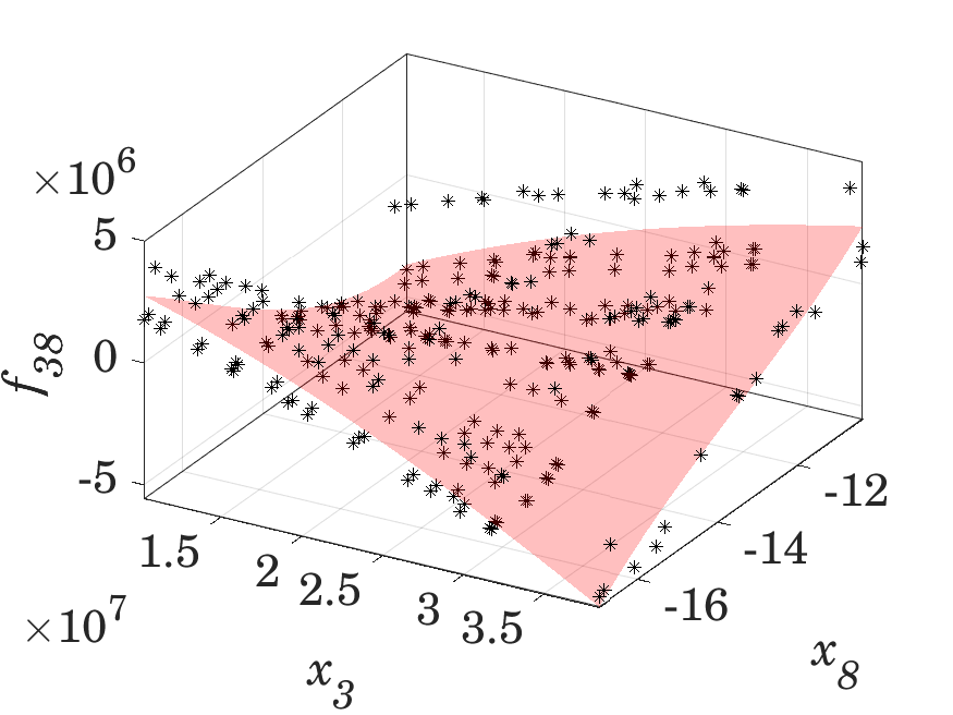
(a) $f_{38}$

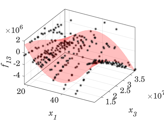
(b) $f_{13}$

(c) $f_{16}$

(d) $f_{17}$

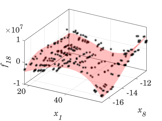
(e) $f_{18}$

Figure 22. Dominant second-order Sobol functions for minimum horizontal stress at Point 5

Among the dominant variables, production pressure and fracture half-length have a considerable impact on the minimum horizontal stress at this point. Using the functions in Figures 21 and 22, the ROM for minimum horizontal stress at Point 5 can be presented as follows:

$$f_{0}= \;A_{0}$$ (5.7a)

$$f_{1}= \;A_{1}-A_{2}\;\cos(A_{0}\;a)+A_{3}\;\sin(A_{0}\;a)+A_{4}\;\cos(2\;A_{0}\;a)+A_{5}\;\sin(2\;A_{0}\;a)+A_{6}\;\cos(3\;A_{0}\;a)+$$

$$A_{7}\;\sin(3\;A_{0}\;a)+A_{8}\;\cos(4\;A_{0}\;a)+A_{9}\;\sin(4\;A_{0}\;a)$$ (5.7b)

$$f_{3}= \;A_{0}\;p_{f}-A_{1}$$ (5.7c)

$$f_{5}= \;-A_{0}\;\nu_{u}+A_{1}$$ (5.7d)

$$f_{6}= \;A_{0}\;\nu-A_{1}$$ (5.7e)

$$f_{7}= \;-A_{0}\;B^{2}+A_{1}\;B-A_{2}$$ (5.7f)

$$f_{8}= \;A_{0}\;\sin(A_{1}\;\kappa+A_{2})+A_{3}\;\sin(A_{4}\;\kappa+A_{5})$$ (5.7g)

$$f_{38}= \;-A_{0}+A_{1}\;p_{f}-A_{2}\;\kappa-A_{3}\;p_{f}^{2}+A_{4}\;p_{f}\kappa+A_{5}\;\kappa^{2}+A_{6}\;p_{f}^{3}+A_{7}\;p_{f}^{2}\;\kappa-A_{8}\;p_{f}\;\kappa^{2}+A_{9}\;\kappa^{3}$$ (5.7h)

$$f_{13}= -A_{0}-A_{1}\;a+A_{2}\;p_{f}+A_{3}\;a^{2}+A_{4}\;a\;p_{f}+-A_{5}\;p_{f}^{2}+A_{6}\;a^{3}-A-7\;a^{2}\;p_{f}-A_{8}\;a\;p_{f}^{2}$$

$$-A_{9}\;p_{f}^{3}-A_{10}\;a^{4}A_{11}\;a^{3}\;p_{f}+A_{12}\;a^{2}\;p_{f}^{2}-A_{13}\;a\;p_{f}^{3}+A_{1}4\;p_{f}^{4}$$ (5.7i)

$$f_{16}= A_{0}-A_{1}\;a+A_{2}\;\nu+A_{3}\;a^{2}+A_{4}\;a\;\nu-A_{5}\;\nu^{2}+A_{6}\;a^{3}-A_{7}\;a^{2}\;\nu-A_{8}\;a\;\nu^{2}+A_{9}\;\nu^{3}$$ (5.7j)

$$f_{17}= -A_{0}-A_{1}\;a+A_{2}\;B+A_{3}\;a^{2}+A_{4}\;a\;B+A_{5}\;B^{2}+A_{6}\;a^{3}-A_{7}\;a^{2}\;B-A_{8}\;a\;B^{2}-A_{9}\;B^{3}$$

$$-A_{10}\;a^{4}-A_{11}\;a^{3}\;B+A_{12}\;a^{2}\;B^{2}-A_{13}\;a\;B^{3}-A_{14}\;B^{4}$$ (5.7k)

$$f_{18}= -A_{0}-A_{1}\;a-A_{2}\;\kappa+A_{3}\;a^{2}+A_{4}\;a\;\kappa+A_{5}\;\kappa^{2}+A_{6}\;a^{3}+A_{7}\;a^{2}\;\kappa+A_{8}\;a\;\kappa^{2}+A_{9}\;\kappa^{3}-$$

$$A_{10}\;a^{4}+A_{11}\;a^{3}\;\kappa-A_{12}\;a^{2}\;\kappa^{2}-A_{13}\;a\;\kappa^{3}-A_{14}\;\kappa^{4}$$ (5.7l)

The coefficients of the functions in Equations (5.7a)–(5.7l) are presented in Tables 8 and 9. Depending on the desired degree of confidence, the ROM in Equations (5.7a)–(5.7l) may be truncated to have smaller number of variables.

Maximum horizontal stress.

The dominant affecting variables to the changes in maximum horizontal stress at point 5 are $p_{f}$, $\nu_{u}$, $\nu$, $B$, $\kappa$, and $f_{18}$. Figure 23 shows the plot of these variables and their corresponding Sobol function.

(a) $f3$

(b) $f5$

(c) $f6$

(d) $f7$

(e) $f8$

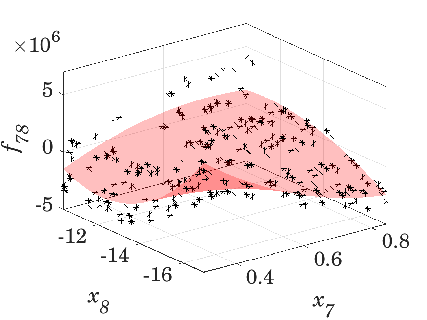
(f) $f_{18}$

Figure 23. Dominant Sobol functions for maximum horizontal stress at Point 5

Using these functions, the following reduced order model may be constructed for maximum horizontal stress:

$$f_{0}= \;A_{0}$$ (5.8a)

$$f_{3}= \;A_{0}\;p_{f}-A_{1}$$ (5.8b)

$$f_{5}= \;-A_{0}\;\nu_{u}+A_{1}$$ (5.8c)

$$f_{6}= \;A_{0}\;\nu-A_{1}$$ (5.8d)

$$f_{7}= \;A_{0}\;B^{3}-A_{1}\;B^{2}+A_{2}\;B-A_{3}$$ (5.8e)

$$f_{8}= \;A_{1}-A_{2}\;\cos(A_{0}\;\kappa)+A_{3}\;\sin(A_{0}\;\kappa)+A_{4}\;\cos(2\;A_{0}\;\kappa)-A_{5}\;\sin(2\;A_{0}\;\kappa)$$ (5.8f)

$$f_{18}= \;-A_{0}-A_{1}\;a+A_{2}\;\kappa+A_{3}\;a^{2}+A_{4}\;a\;\kappa+A_{5}\;\kappa^{2}+A_{6}\;a^{3}+A_{7}\;a^{2}\;\kappa+A_{8}\;a\;\kappa^{2}-A_{9}\;\kappa^{3}-A_{10}\;a^{4}$$

$$-A_{11}\;a^{3}\;\kappa+A{12}\;a^{2}\;\kappa^{2}-A_{13}\;a\;\kappa^{3}-A_{14}\;\kappa^{4}$$ (5.8g)

Coefficients of the functions in Equations (5.8a)–(5.8g) are presented in Table 10. Next point that we investigate in this paper is Point 6 which is located close to horizontal well and in the middle of pre-existing fracture’s spacing.

5.3. Sobol functions and ROM at Point 6

Point 6 is the most important point among all other points for refracturing process because it is the point were the refracture will be placed. Therefore, it is important to keep track of the changes in pore pressure, maximum horizontal, and minimum horizontal stresses at this point.

Pore pressure.

There are four main Sobol indices that control the changes of the pore pressure at Point 6. These inputs are $S_{3}$, $S_{8}$ $S_{38}$, and $S_{48}$. Figure 24 shows the dominant Sobol functions for pore pressure at Point 6.

(a) $f_{3}$

(b) $f_{8}$

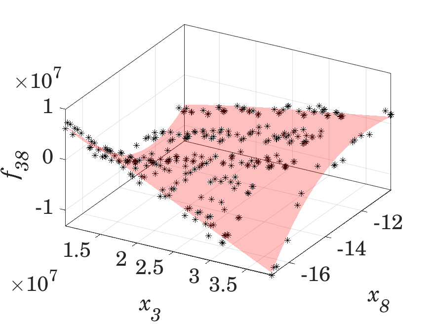
(c) $f_{38}$

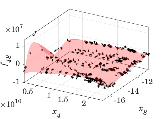
(d) $f_{48}$

Figure 24. Dominant Sobol functions for pore pressure at Point 6

The reduced order model for pore pressure at Point 6 can be represented as:

$$f_{0}= \;A_{0}$$ (5.9a)

$$f_{1}= \;A_{0}\;p_{f}-A_{1}$$ (5.9b)

$$f_{8}= \;A_{0}\;\sin(A_{1}\;\kappa+A_{2})+A_{3}\;\sin(A_{4}\;\kappa-A_{5})$$ (5.9c)

$$f_{38}= \;-A_{0}+A_{1}\;a-A_{2}\;\kappa-A_{3}\;a^{2}+A_{4}\;a\;\kappa+A_{5}\;\kappa^{2}+A_{6}\;a^{3}-A_{7}\;a^{2}\;\kappa-A_{8}\;a\;\kappa^{2}+A_{9}\;\kappa^{3}$$ (5.9d)

$$f_{48}= \;-A_{0}+A_{1}\;G+A_{2}\;\kappa-A_{3}\;G^{2}+A_{4}\;G\;\kappa+A_{5}\;\kappa^{2}-A_{6}\;G^{3}-A_{7}\;G^{2}\;\kappa-A_{8}\;G\;\kappa^{2}$$ (5.9e)

$$-A_{9}\;\kappa^{3}+A_{10}\;G^{4}+A_{11}\;G^{3}\;\kappa-A_{12}\;G^{2}\;\kappa^{2}-A_{13}\;G\;\kappa^{3}-A_{14}\;\kappa^{4}+A_{15}\;G^{5}$$ (5.9f)

$$-A_{16}\;G^{4}\;\kappa+A_{17}\;G^{3}\;\kappa^{2}+A_{18}\;G^{2}\;\kappa^{3}+A_{19}\;G\;\kappa^{4}-A_{20}\;\kappa^{5}$$ (5.9g)

Coefficients of the functions in Equations (5.9a)–(5.9g) are presented in Table 11.

Minimum horizontal stress.

There are two dominant input variables that contribute to more than $65\%$ of the changes in minimum horizontal stress at Point 6. These two variables are fracture half-length and the interaction effect of the fracture half-length and fracture spacing. About half of the changes in the minimum horizontal stress is due to changes of these two variables (i.e., combination effect). Figure 25 shows the plots of these two variables and their corresponding functions.

(a) $f_{1}$

(b) $f_{12}$

Figure 25. Dominant Sobol functions for minimum horizontal stress at Point 6.

Based on the plots of the dominant Sobol function for minimum horizontal stress at Point 6, the reduced order model for $\sigma_{h}$ at this point may be obtained using:

$$f_{0}= \;5.53\times 10^{7}$$ (5.10a)

$$f_{1}= \;-A_{0}\;a^{8}+A_{1}\;a^{7}-A_{2}\;a^{6}+A_{3}\;a^{5}+A_{4}\;a^{4}-A_{5}\;a^{3}-A_{6}\;a^{2}-A_{7}\;a-A_{8}$$ (5.10b)

$$f_{12}= \;-A_{0}+A_{1}\;a-A_{2}\;b+A_{3}\;a^{2}-A_{4}\;a\;b+A_{5}\;b^{2}-A_{6}\;a^{3}+A_{7}\;a^{2}\;b+A_{8}\;a\;b^{2}-A_{9}\;b^{3}$$ (5.10c)

Coefficients of the functions in Equations (5.10a)–(5.10c) are presented in Table 12

Maximum horizontal stress.

There are seven dominant contributors to the changes in maximum horizontal stress at Point 6. These contributors are fracture half-length, production pressure, undrained Poisson’s ratio, drained Poisson’s ratio, Skemptson’s coefficient, mobility, and interaction of fracture half-length and mobility. Figure 26 shows plots of these contributors and their corresponding Sobol functions.

(a) $f_{1}$

(b) $f_{3}$

(c) $f_{5}$

(d) $f_{6}$

(e) $f_{7}$

(f) $f_{8}$

(g) $f_{18}$

Figure 26. Dominant Sobol functions for maximum horizontal stress at Point 6

Using the functions in Figure 26, the following ROM can be used to calculate the maximum horizontal stress at Point 6:

$$f_{0}= \;A_{0}$$ (5.11a)

$$f_{1}= \;-A_{0}\;a^{2}+A_{1}\;a-A_{2}$$ (5.11b)

$$f_{3}= \;A_{0}\;p_{f}-A_{1}$$ (5.11c)

$$f_{5}= \;-A_{0}\;\nu_{u}+A_{1}$$ (5.11d)

$$f_{6}= \;A_{0}\;\nu-A_{1}$$ (5.11e)

$$f_{7}= \;-A_{0}\;B^{2}+A_{1}\;B-A_{2}$$ (5.11f)

$$f_{8}= \;A_{0}\;\sin(A_{1}\;\kappa+A_{2})+A_{3}\;\sin(A_{4}\;\kappa-A_{5})+A_{6}\;\sin(A_{7}\;\kappa+A_{8})$$ (5.11g)

$$f_{18}= \;-A_{0}-A_{1}\;a-A_{2}\;\kappa-A_{3}\;a^{2}+A_{4}\;a\;\kappa+A_{5}\;\kappa^{2}+A_{6}\;a^{3}-A_{7}\;a^{2}\;\kappa+A_{8}\;a\;\kappa^{2}-A_{9}\;\kappa^{3}$$ (5.11h)

The coefficients of the functions in Equations (5.11a)–(5.11h)are presented in Table 12. In this section, different reduced order models were presented for calculating the pore pressure, maximum horizontal stress and minimum horizontal stress at different points around a hydraulically-fractured horizontal well. Presented ROMs are valid for the case of one year production with constant production pressure. for any other point or a different time, a set of new ROM may be constructed using the same procedure. It also showed that depending on the location of the desired point with respect to the horizontal well and pre-existing hydraulic fractures, different set of dominant variables contribute to the changes of the desired quantity (i.e., pore pressure or stresses). As an example, we presented the ROM for the points that are located outside the spacing, at the tip in the hypothetical line connecting the tips of fractures, and in the middle line between fractures.

6. CONCLUDING REMARKS

In this study, using a fully-coupled geomechanical model, it was shown that different hydraulically-fractured rocks have dissimilar pore pressure depletion and stress change under the same boundary conditions. This dissimilarity is illustrated using two parallel hydraulic fractures after varying production time periods. Results show that, besides the different behaviors that were observed for different rocks, the changes in the mentioned variables were different from point to point around hydraulic fractures for the same rock type. To find the most influencing inputs on the model outputs, a global sensitivity analysis based on Sobol method is used. We chose eight parameters as our set of input parameters. Pore pressure, maximum horizontal stress, and minimum horizontal stress were chosen as the quantities of interests.

The results showed that mobility $\kappa$ and production pressure $p_{f}$ (which needs to be seen as $\Delta p$ between reservoir and fracture) and their interactions are the dominant properties that cause most of the pore pressure changes. These two variables are also dominant for the changes in minimum and maximum horizontal stresses. It was observed that as the point of observation gets closer to the spacing between fractures, fracture half-length and its interactions contribute to $20\%$ of the changes in pore pressure depletion. Moreover, it was observed that interaction between fracture half-length and fracture spacing ($S_{12}$) has the most significant impact on the minimum horizontal stress at a point inside the spacing. Thus, selecting these two variables appropriately will increase the chance of success in operations such as refracturing.

The following inferences are valuable for practical applications. Different input variables are dominant responsible elements for variation of different output variables. The dominant factors are not the same with time and location. Thus, in order to perform any further operation around a hydraulically-fractured well-bore, time and location have to be considered carefully. The Sobol method offers a nice framework for a systematic parametric study, as it can capture not only the influence of individual parameters but also the influence of interactions among the parameters.

Finally, we suggest three plausible future works. The first research effort can be towards combining fracture modeling with double porosity/permeability models (Nakshatrala et al, 2018; Joodat et al, 2018). The second effort is to incorporate inertial effects (e.g., Forchheimer-type models) and pressure-dependence viscosity (Chang et al, 2017; Mapakshi et al, 2018) on the hydraulic fracture propagation. The third effort can be towards utilizing phase modeling for hydraulic fracture propagation on the lines similar to (Miehe et al, 2010).

Appendix A COEFFICIENTS OF THE REDUCED ORDER MODELS

Table 4. Coefficients of the reduced order model for pore pressure at Point 1 (Equations (5.2a)–(5.2d))

Coeff	$f_{0}$	$f_{3}$	$f_{8}$	$f_{38}$
$A_{0}$	$4.01\times 10^{7}$	$0.2348$	$8.9\times 10^{6}$	$1.161\times 10^{6}$
$A_{1}$	$-$	$2.93\times 10^{6}$	$0.43$	$4.734\times 10^{5}$
$A_{2}$	$-$	$-$	$2.165$	$6718$
$A_{3}$	$-$	$-$	$7.8\times 10^{5}$	$1.856\times 10^{5}$
$A_{4}$	$-$	$-$	$1.7$	$1.995\times 10^{6}$
$A_{5}$	$-$	$-$	$0.14$	$1.667\times 10^{5}$
$A_{6}$	$-$	$-$	$-$	$1408$
$A_{7}$	$-$	$-$	$-$	$1664$
$A_{8}$	$-$	$-$	$-$	$5.835\times 10^{5}$
$A_{9}$	$-$	$-$	$-$	$4.631\times 10^{4}$

Table 5. Coefficients of the reduced order model for the minimum horizontal stress at Point 1 (Equations (5.3a)–(5.3g))

Coeff	$f_{0}$	$f_{3}$	$f_{5}$	$f_{6}$	$f_{7}$	$f_{8}$	$f_{38}$
$A_{0}$	$5.13\times 10^{7}$	$0.1284$	$1.117\times 10^{7}$	$8.878\times 10^{6}$	$1.508\times 10^{7}$	$1.236\times 10^{6}$	$4.47\times 10^{5}$
$A_{1}$	$-$	$2.248\times 10^{6}$	$5.529\times 10^{6}$	$2.898\times 10^{5}$	$3.305\times 10^{7}$	$0.9195$	$1.404\times 10^{5}$
$A_{2}$	$-$	$-$	$-$	$-$	$2.656$	$2.074$	$1.442\times 10^{5}$
$A_{3}$	$-$	$-$	$-$	$-$	$5.05\times 10^{6}$	$6.497\times 10^{6}$	$1.806\times 10^{5}$
$A_{4}$	$-$	$-$	$-$	$-$	$-$	$0.1707$	$9.587\times 10^{5}$
$A_{5}$	$-$	$-$	$-$	$-$	$-$	$1.042$	$2.08\times 10^{5}$
$A_{6}$	$-$	$-$	$-$	$-$	$-$	$1.97\times 10^{5}$	$6396$
$A_{7}$	$-$	$-$	$-$	$-$	$-$	$2.26$	$5117$
$A_{8}$	$-$	$-$	$-$	$-$	$-$	$7.68$	$2.532\times 10^{5}$
$A_{9}$	$-$	$-$	$-$	$-$	$-$	$-$	$1.505\times 10^{4}$

Table 6. Coefficients of the reduced order model for the maximum horizontal stress at Point 1 (Equations (5.5a)–(5.5g))

Coeff	$f_{0}$	$f_{3}$	$f_{5}$	$f_{6}$	$f_{7}$	$f_{8}$	$f_{38}$
$A_{0}$	$5.55\times 10^{7}$	$1$	$8.78\times 10^{6}$	$2.933\times 10^{7}$	$1.392\times 10^{7}$	$1.433\times 10^{6}$	$3.951\times 10^{7}$
$A_{1}$	$-$	$1.604\times 10^{6}$	$4.468\times 10^{6}$	$4.687\times 10^{6}$	$2.93\times 10^{7}$	$0.8957$	$2.278$
$A_{2}$	$-$	$-$	$-$	$9.515\times 10^{5}$	$2.233\times 10^{7}$	$1.726$	$4.13\times 10^{6}$
$A_{3}$	$-$	$-$	$-$	$-$	$4.276\times 10^{6}$	$5.315\times 10^{6}$	$0.2681$
$A_{4}$	$-$	$-$	$-$	$-$	$-$	$0.1887$	$7.187\times 10^{4}$
$A_{5}$	$-$	$-$	$-$	$-$	$-$	$0.804$	$1797$
$A_{6}$	$-$	$-$	$-$	$-$	$-$	$2.289\times 10^{5}$	$-$
$A_{7}$	$-$	$-$	$-$	$-$	$-$	$2.185$	$-$
$A_{8}$	$-$	$-$	$-$	$-$	$-$	$6.766$	$-$

Table 7. Coefficients of the reduced order model for pore pressure at Point 5 (Equations (5.6a)–(5.6e))

Coeff	$f_{0}$	$f_{1}$	$f_{3}$	$f_{8}$	$f_{38}$
$A_{0}$	$3.23\times 10^{7}$	$3439$	$0.5258$	$2.939\times 10^{7}$	$3.526\times 10^{6}$
$A_{1}$	$-$	$5929$	$9.196\times 10^{6}$	$0.107$	$1.341\times 10^{6}$
$A_{2}$	$-$	$9.585\times 10^{6}$	$-$	$1.871$	$5.341\times 10^{5}$
$A_{3}$	$-$	$-$	$-$	$2.294\times 10^{6}$	$2.164\times 10^{5}$
$A_{4}$	$-$	$-$	$-$	$1.085$	$2.553\times 10^{6}$
$A_{5}$	$-$	$-$	$-$	$0.06293$	$5.576\times 10^{5}$
$A_{6}$	$-$	$-$	$-$	$4.435\times 10^{5}$	$3049$
$A_{7}$	$-$	$-$	$-$	$2.071$	$1.674\times 10^{4}$
$A_{8}$	$-$	$-$	$-$	$2.674$	$7.557\times 10^{5}$
$A_{9}$	$-$	$-$	$-$	$-$	$1.106\times 10^{5}$

Table 8. Coefficients of the first order Sobol functions for the minimum horizontal stress at Point 5 (Equations (5.7a)–(5.7g)).

Coeff	$f_{0}$	$f_{1}$	$f_{3}$	$f_{5}$	$f_{6}$	$f_{7}$	$f_{8}$
$A_{0}$	$4.75\times 10^{7}$	$0.1193$	$0.2848$	$2.227\times 10^{7}$	$1.8\times 10^{7}$	$1.58\times 10^{7}$	$1.38\times 10^{6}$
$A_{1}$	$-$	$1.95\times 10^{6}$	$5.914\times 10^{6}$	$1.066\times 10^{7}$	$1.146\times 10^{6}$	$2.802\times 10^{7}$	$1.191$
$A_{2}$	$-$	$8.279\times 10^{5}$	$-$	$-$	$-$	$8.152\times 10^{6}$	$1.187$
$A_{3}$	$-$	$4.604\times 10^{6}$	$-$	$-$	$-$	$-$	$7.738\times 10^{6}$
$A_{4}$	$-$	$9.287\times 10^{5}$	$-$	$-$	$-$	$-$	$0.298$
$A_{5}$	$-$	$2.434\times 10^{6}$	$-$	$-$	$-$	$-$	$0.6055$
$A_{6}$	$-$	$8.653\times 10^{5}$	$-$	$-$	$-$	$-$	$-$
$A_{7}$	$-$	$1.009\times 10^{6}$	$-$	$-$	$-$	$-$	$-$
$A_{8}$	$-$	$3.608\times 10^{5}$	$-$	$-$	$-$	$-$	$-$
$A_{9}$	$-$	$2.868\times 10^{5}$	$-$	$-$	$-$	$-$	$-$

Table 9. Coefficients of the second order Sobol functions for the minimum horizontal stress at Point 5 (Equations (5.7h)–(5.7l)).

Coeff	$f_{38}$	$f_{13}$	$f_{16}$	$f_{17}$	$f_{18}$
$A_{0}$	$9.637\times 10^{5}$	$1.123\times 10^{6}$	$1.06\times 10^{7}$	$1.154\times 10^{6}$	$3.744\times 10^{6}$
$A_{1}$	$9.514\times 10^{4}$	$4.399\times 10^{5}$	$1.284\times 10^{6}$	$7.664\times 10^{5}$	$1.954\times 10^{6}$
$A_{2}$	$4.621\times 10^{5}$	$1.114\times 10^{6}$	$9.594\times 10^{7}$	$1.28\times 10^{6}$	$2.229\times 10^{6}$
$A_{3}$	$2.127\times 10^{5}$	$5.819\times 10^{5}$	$1.082\times 10^{4}$	$3.21\times 10^{5}$	$1.827\times 10^{6}$
$A_{4}$	$1.347\times 10^{6}$	$1.24\times 10^{6}$	$7.181\times 10^{6}$	$1.673\times 10^{6}$	$1.111\times 10^{5}$
$A_{5}$	$3.006\times 10^{5}$	$9.329\times 10^{5}$	$1.228\times 10^{9}$	$1.64\times 10^{5}$	$1.796\times 10^{6}$
$A_{6}$	$1.411\times 10^{4}$	$9.442\times 10^{4}$	$99.63$	$2.329\times 10^{5}$	$4.715\times 10^{5}$
$A_{7}$	$4099$	$8.217\times 10^{5}$	$9.425\times 10^{4}$	$9.159\times 10^{5}$	$1.76\times 10^{6}$
$A_{8}$	$1.667\times 10^{5}$	$1.604\times 10^{4}$	$3.635\times 10^{5}$	$7.561\times 10^{4}$	$7.387\times 10^{5}$
$A_{9}$	$2.057\times 10^{5}$	$1.432\times 10^{5}$	$2.268\times 10^{9}$	$1.482\times 10^{5}$	$1.013\times 10^{5}$
$A_{10}$	$-$	$9.507\times 10^{4}$	$-$	$1.409\times 10^{5}$	$2.414\times 10^{5}$
$A_{11}$	$-$	$6.673\times 10^{5}$	$-$	$8.554\times 10^{5}$	$9.83\times 10^{5}$
$A_{12}$	$-$	$8912$	$-$	$4.41\times 10^{5}$	$7.301\times 10^{5}$
$A_{13}$	$-$	$152.3$	$-$	$4.697\times 10^{4}$	$8.411\times 10^{5}$
$A_{14}$	$-$	$2.301\times 10^{5}$	$-$	$1.566\times 10^{5}$	$3.61\times 10^{5}$

Table 10. Coefficients of the reduced order model for the maximum horizontal stress at Point 5 (Equations (5.8a)–(5.8g))

Coeff	$f_{0}$	$f_{3}$	$f_{5}$	$f_{6}$	$f_{7}$	$f_{8}$	$f_{18}$
$A_{0}$	$5.05\times 10^{7}$	$0.339$	$3.209\times 10^{7}$	$2.718\times 10^{7}$	$2.28\times 10^{7}$	$0.6016$	$1.434\times 10^{6}$
$A_{1}$	$-$	$8.31\times 10^{6}$	$1.293\times 10^{7}$	$4.38\times 10^{6}$	$6\times 10^{7}$	$1.648\times 10^{6}$	$1.274\times 10^{6}$
$A_{2}$	$-$	$-$	$-$	$-$	$5.831\times 10^{7}$	$3.453\times 10^{6}$	$2.579\times 10^{5}$
$A_{3}$	$-$	$-$	$-$	$-$	$1.648\times 10^{7}$	$2.723\times 10^{6}$	$7.189\times 10^{5}$
$A_{4}$	$-$	$-$	$-$	$-$	$-$	$1.789\times 10^{4}$	$2.978\times 10^{6}$
$A_{5}$	$-$	$-$	$-$	$-$	$-$	$1.512\times 10^{6}$	$1.117\times 10^{6}$
$A_{6}$	$-$	$-$	$-$	$-$	$-$	$-$	$3.386\times 10^{4}$
$A_{7}$	$-$	$-$	$-$	$-$	$-$	$-$	$6.242\times 10^{4}$
$A_{8}$	$-$	$-$	$-$	$-$	$-$	$-$	$7.895\times 10^{5}$
$A_{9}$	$-$	$-$	$-$	$-$	$-$	$-$	$4.039\times 10^{4}$
$A_{10}$	$-$	$-$	$-$	$-$	$-$	$-$	$2.015\times 10^{5}$
$A_{11}$	$-$	$-$	$-$	$-$	$-$	$-$	$4.165\times 10^{5}$
$A_{12}$	$-$	$-$	$-$	$-$	$-$	$-$	$1.227\times 10^{5}$
$A_{13}$	$-$	$-$	$-$	$-$	$-$	$-$	$1.066\times 10^{6}$
$A_{14}$	$-$	$-$	$-$	$-$	$-$	$-$	$3.404\times 10^{5}$

Table 11. Coefficients of the reduced order model for the pore pressure at Point 6 (Equations (5.9a) - (5.9g))

Coeff	$f_{0}$	$f_{1}$	$f_{8}$	$f_{38}$	$f_{48}$
$A_{0}$	$2.65\times 10^{7}$	$0.824$	$1.44\times 10^{8}$	$3.644\times 10^{6}$	$3.201\times 10^{6}$
$A_{1}$	$-$	$1.789\times 10^{7}$	$0.4676$	$2.137\times 10^{6}$	$8.985\times 10^{5}$
$A_{2}$	$-$	$-$	$2.499$	$1.057\times 10^{6}$	$6.924\times 10^{5}$
$A_{3}$	$-$	$-$	$1.352\times 10^{8}$	$1.295\times 10^{5}$	$1.588\times 10^{6}$
$A_{4}$	$-$	$-$	$0.5053$	$2.476\times 10^{6}$	$2.344\times 10^{6}$
$A_{5}$	$-$	$-$	$6.469$	$7.658\times 10^{5}$	$3.294\times 10^{6}$
$A_{6}$	$-$	$-$	$-$	$6.063\times 10^{4}$	$9.518\times 10^{5}$
$A_{7}$	$-$	$-$	$-$	$1060$	$1.285\times 10^{6}$
$A_{8}$	$-$	$-$	$-$	$1.79\times 10^{6}$	$4.197\times 10^{6}$
$A_{9}$	$-$	$-$	$-$	$3.814\times 10^{5}$	$3.788\times 10^{4}$
$A_{10}$	$-$	$-$	$-$	$-$	$8.773\times 10^{5}$
$A_{11}$	$-$	$-$	$-$	$-$	$2.672\times 10^{4}$
$A_{12}$	$-$	$-$	$-$	$-$	$1.711\times 10^{5}$
$A_{13}$	$-$	$-$	$-$	$-$	$1.057\times 10^{6}$
$A_{14}$	$-$	$-$	$-$	$-$	$9.727\times 10^{5}$
$A_{15}$	$-$	$-$	$-$	$-$	$3.976\times 10^{5}$
$A_{16}$	$-$	$-$	$-$	$-$	$2.538\times 10^{4}$
$A_{17}$	$-$	$-$	$-$	$-$	$1.006\times 10^{5}$
$A_{18}$	$-$	$-$	$-$	$-$	$7.33\times 10^{5}$
$A_{19}$	$-$	$-$	$-$	$-$	$1.885\times 10^{6}$
$A_{20}$	$-$	$-$	$-$	$-$	$2.617\times 10^{5}$

Table 12. Coefficients of the reduced order model for the minimum horizontal stress at Point 6 (Equations (5.10a)–(5.10c))

Coeff	$f_{0}$	$f_{1}$	$f_{12}$
$A_{0}$	$5.53\times 10^{7}$	$5806$	$3.886\times 10^{4}$
$A_{1}$	$-$	$4.612\times 10^{4}$	$3.676\times 10^{4}$
$A_{2}$	$-$	$1.266\times 10^{5}$	$5.765\times 10^{4}$
$A_{3}$	$-$	$1.355\times 10^{5}$	$3.558\times 10^{4}$
$A_{4}$	$-$	$4994$	$1.259\times 10^{5}$
$A_{5}$	$-$	$1.696\times 10^{5}$	$1.47\times 10^{4}$
$A_{6}$	$-$	$2.416\times 10^{5}$	$2.868\times 10^{4}$
$A_{7}$	$-$	$1.984\times 10^{5}$	$5.699\times 10^{4}$
$A_{8}$	$-$	$3.771\times 10^{4}$	$1.4\times 10^{4}$
$A_{9}$	$-$	$-$	$3266$

Table 13. Coefficients of the reduced order model for the maximum horizontal stress at Point 6 (Equations (5.11a)–(5.11h))

Coeff	$f_{0}$	$f_{1}$	$f_{3}$	$f_{5}$	$f_{6}$	$f_{7}$	$f_{8}$	$f_{18}$
$A_{0}$	$5.05\times 10^{7}$	$1708$	$0.335$	$3.19\times 10^{7}$	$2.72\times 10^{7}$	$2.25\times 10^{7}$	$2.565\times 10^{7}$	$2.528\times 10^{6}$
$A_{1}$	$-$	$1.016\times 10^{5}$	$8.67\times 10^{6}$	$1.2\times 10^{7}$	$5.1\times 10^{6}$	$2.565\times 10^{7}$	$1.271$	$3.111\times 10^{5}$
$A_{2}$	$-$	$1.436\times 10^{6}$	$-$	$-$	$-$	$1.46\times 10^{7}$	$3.662$	$3.678\times 10^{4}$
$A_{3}$	$-$	$-$	$-$	$-$	$-$	$-$	$1.506\times 10^{7}$	$4.567\times 10^{4}$
$A_{4}$	$-$	$-$	$-$	$-$	$-$	$-$	$1.411$	$6.293\times 10^{5}$
$A_{5}$	$-$	$-$	$-$	$-$	$-$	$-$	$4.119$	$3.488\times 10^{5}$
$A_{6}$	$-$	$-$	$-$	$-$	$-$	$-$	$1.153\times 10^{7}$	$6.563\times 10^{4}$
$A_{7}$	$-$	$-$	$-$	$-$	$-$	$-$	$1.016$	$1.54\times 10^{5}$
$A_{8}$	$-$	$-$	$-$	$-$	$-$	$-$	$10.12$	$1.734\times 10^{5}$
$A_{9}$	$-$	$-$	$-$	$-$	$-$	$-$	$-$	$4.125\times 10^{4}$

References

- Aliabadi (2002) Aliabadi MH (2002) The boundary element method. Volume 2, Applications in solids and structures. Wiley
- Aliabadi and Rooke (1991) Aliabadi MH, Rooke D (1991) The boundary element method. Numerical Fracture Mechanics pp 90–139
- Archer et al (1997) Archer G, Saltelli A, Sobol I (1997) Sensitivity measures, anova-like techniques and the use of bootstrap. Journal of Statistical Computation and Simulation 58(2):99–120
- Arwade et al (2010) Arwade SR, Moradi M, Louhghalam A (2010) Variance decomposition and global sensitivity for structural systems. Engineering Structures 32(1):1–10
- Auder et al (2012) Auder B, De Crecy A, Iooss B, Marques M (2012) Screening and metamodeling of computer experiments with functional outputs. application to thermal–hydraulic computations. Reliability Engineering & System Safety 107:122–131
- Berchenko and Detournay (1997) Berchenko I, Detournay E (1997) Deviation of hydraulic fractures through poroelastic stress changes induced by fluid injection and pumping. International Journal of Rock Mechanics and Mining Sciences 34(6):1009–1019
- Biot (1941) Biot MA (1941) General theory of three-dimensional consolidation. Journal of applied physics 12(2):155–164
- Bobet and Mutlu (2005) Bobet A, Mutlu O (2005) Stress and displacement discontinuity element method for undrained analysis. Engineering fracture mechanics 72(9):1411–1437
- Borgonovo and Plischke (2016) Borgonovo E, Plischke E (2016) Sensitivity analysis: a review of recent advances. European Journal of Operational Research 248(3):869–887
- Brebbia et al (2012) Brebbia CA, Telles JCF, Wrobel LC (2012) Boundary element techniques: theory and applications in engineering. Springer Science & Business Media
- Carvalho (1991) Carvalho JL (1991) Poroelastic effects and influence of material interfaces on hydraulic fracture behaviour. PhD thesis, University of Toronto
- Chadwick (2012) Chadwick P (2012) Continuum mechanics: concise theory and problems. Courier Corporation
- Chang et al (2017) Chang J, Nakshatrala KB, Reddy JN (2017) Modification to Darcy-Forchheimer model due to pressure-dependent viscosity: consequences and numerical solutions. Journal of Porous Media 20(3)
- Cheng (2016) Cheng AHD (2016) Poroelasticity, vol 27. Springer, switzerland
- Chun (2013) Chun KH (2013) Thermo-poroelastic fracture propagation modeling with displacement discontinuity boundary element method. PhD thesis, Texas A&M University
- Cleary (1977) Cleary MP (1977) Fundamental solutions for a fluid-saturated porous solid. International Journal of Solids and Structures 13(9):785–806
- Crouch (1976) Crouch S (1976) Solution of plane elasticity problems by the displacement discontinuity method. i. infinite body solution. International Journal for Numerical Methods in Engineering 10(2):301–343
- Cruse (2012) Cruse TA (2012) Boundary element analysis in computational fracture mechanics, vol 1. Springer Science & Business Media
- Curran and Carvalho (1987) Curran J, Carvalho JL (1987) A displacement discontinuity model for fluid-saturated porous media. In: 6th ISRM Congress, International Society for Rock Mechanics
- Dai et al (2014) Dai C, Li H, Zhang D (2014) Efficient and accurate global sensitivity analysis for reservoir simulations by use of probabilistic collocation method. SPE Journal 19(04):621–635
- Detournay and Cheng (1987) Detournay E, Cheng AH (1987) Poroelastic solution of a plane strain point displacement discontinuity. Journal of applied mechanics 54(4):783–787
- Detournay et al (1989) Detournay E, Cheng AD, Roegiers JC, Mclennan JD (1989) Poroelasticity considerations in in situ stress determination by hydraulic fracturing. In: International Journal of Rock Mechanics and Mining Sciences & Geomechanics Abstracts, Elsevier, vol 26, pp 507–513
- Herman and Usher (2017) Herman J, Usher W (2017) Salib: an open-source python library for sensitivity analysis. The Journal of Open Source Software 2(9)
- Hill and Tiedeman (2006) Hill MC, Tiedeman CR (2006) Effective groundwater model calibration: with analysis of data, sensitivities, predictions, and uncertainty. John Wiley & Sons
- Iooss and Lemaître (2015) Iooss B, Lemaître P (2015) A review on global sensitivity analysis methods. In: Uncertainty management in simulation-optimization of complex systems, Springer, pp 101–122
- Joodat et al (2018) Joodat SHS, Nakshatrala KB, Ballarini R (2018) Modeling flow in porous media with double porosity/permeability: A stabilized mixed formulation, error analysis, and numerical solutions. Computer Methods in Applied Mechanics and Engineering 337:632–676
- Lefebvre et al (2010) Lefebvre S, Roblin A, Varet S, Durand G (2010) A methodological approach for statistical evaluation of aircraft infrared signature. Reliability Engineering & System Safety 95(5):484–493
- Liu and Li (2014) Liu Y, Li Y (2014) Revisit of the equivalence of the displacement discontinuity method and boundary element method for solving crack problems. Engineering Analysis with Boundary Elements 47:64–67
- Makowski et al (2006) Makowski D, Naud C, Jeuffroy MH, Barbottin A, Monod H (2006) Global sensitivity analysis for calculating the contribution of genetic parameters to the variance of crop model prediction. Reliability Engineering & System Safety 91(10-11):1142–1147
- Mapakshi et al (2018) Mapakshi NK, Chang J, Nakshatrala KB (2018) A scalable variational inequality approach for flow through porous media models with pressure-dependent viscosity. Journal of Computational Physics 359:137–163
- Mathias et al (2010) Mathias SA, Tsang CF, van Reeuwijk M (2010) Investigation of hydromechanical processes during cyclic extraction recovery testing of a deformable rock fracture. International Journal of Rock Mechanics and Mining Sciences 47(3):517–522
- Miehe et al (2010) Miehe C, Welschinger F, Hofacker M (2010) Thermodynamically consistent phase-field models of fracture: Variational principles and multi-field FE implementations. International Journal for Numerical Methods in Engineering 83(10):1273–1311
- Nakshatrala et al (2018) Nakshatrala KB, Joodat SHS, Ballarini R (2018) Modeling flow in porous media with double porosity/permeability: Mathematical model, properties, and analytical solutions. Journal of Applied Mechanics 85(8):081,009
- Nashawi et al (2010) Nashawi IS, Malallah A, Al-Bisharah M (2010) Forecasting world crude oil production using multicyclic hubbert model. Energy & Fuels 24(3):1788–1800
- Oliver and Chen (2011) Oliver DS, Chen Y (2011) Recent progress on reservoir history matching: a review. Computational Geosciences 15(1):185–221
- Ozkan et al (2009) Ozkan E, Brown ML, Raghavan RS, Kazemi H (2009) Comparison of fractured horizontal-well performance in conventional and unconventional reservoirs. In: SPE Western Regional Meeting, Society of Petroleum Engineers
- Pianosi et al (2016) Pianosi F, Beven K, Freer J, Hall JW, Rougier J, Stephenson DB, Wagener T (2016) Sensitivity analysis of environmental models: A systematic review with practical workflow. Environmental Modelling & Software 79:214–232
- Rezaei et al (2017a) Rezaei A, Rafiee M, Bornia G, Soliman M, Morse S (2017a) Protection refrac: Analysis of pore pressure and stress change due to refracturing of legacy wells. In: Unconventional Resources Technology Conference, Society of Petroleum Engineers
- Rezaei et al (2017b) Rezaei A, Rafiee M, Bornia G, Soliman M, Siddiqui F (2017b) The role of pore pressure depletion in propagation of new hydraulic fractures during refaracturing of horizontal wells. In: SPE Annual Technical Conference and Exhibition, Society of Petroleum Engineers
- Rezaei et al (2018) Rezaei A, Bornia G, Rafiee M, Soliman M, Morse S (2018) Analysis of refracturing in horizontal wells: Insights from the poroelastic displacement discontinuity method. International Journal for Numerical and Analytical Methods in Geomechanics pp 1–22
- Rice and Cleary (1976) Rice JR, Cleary MP (1976) Some basic stress diffusion solutions for fluid-saturated elastic porous media with compressible constituents. Reviews of Geophysics 14(2):227–241
- Roussel and Sharma (2012) Roussel NP, Sharma MM (2012) Role of stress reorientation in the success of refracture treatments in tight gas sands. SPE Production & Operations 27(04):346–355
- Safari et al (2015) Safari R, Lewis RE, Ma X, Mutlu U, Ghassemi A (2015) Fracture curving between tightly spaced horizontal wells. In: Unconventional Resources Technology Conference, San Antonio, Texas, 20-22 July 2015, Society of Exploration Geophysicists, American Association of Petroleum Geologists, Society of Petroleum Engineers, pp 493–509
- Saltelli et al (2004) Saltelli A, Tarantola S, Campolongo F, Ratto M (2004) Sensitivity analysis in practice: a guide to assessing scientific models. John Wiley & Sons
- Saltelli et al (2008) Saltelli A, Ratto M, Andres T, Campolongo F, Cariboni J, Gatelli D, Saisana M, Tarantola S (2008) Global sensitivity analysis: the primer. John Wiley & Sons
- Sobol (1993) Sobol IM (1993) Sensitivity estimates for nonlinear mathematical models. Mathematical modelling and computational experiments 1(4):407–414
- Sobol (2001) Sobol IM (2001) Global sensitivity indices for nonlinear mathematical models and their monte carlo estimates. Mathematics and computers in simulation 55(1-3):271–280
- Soliman and Dusterhoft (2016) Soliman MY, Dusterhoft R (2016) Fracturing Horizontal Wells. McGraw Hill Professional
- Soliman et al (2006) Soliman MY, Pongratz R, Rylance M, Prather D (2006) Fracture treatment optimization for horizontal well completion. In: paper SPE 102616 presented at the SPE Russian Oil and Gas Technical Conference and Exhibition, Moscow, Russia, pp 3–6
- Tian (2013) Tian W (2013) A review of sensitivity analysis methods in building energy analysis. Renewable and Sustainable Energy Reviews 20:411–419
- Vandamme et al (1989) Vandamme L, Detournay E, Cheng AD (1989) A two-dimensional poroelastic displacement discontinuity method for hydraulic fracture simulation. International Journal for Numerical and Analytical Methods in Geomechanics 13(2):215–224
- Verde (2015) Verde A (2015) Global sensitivity analysis of geomechanical fractured reservoir parameters. In: 49th US Rock Mechanics/Geomechanics Symposium, American Rock Mechanics Association
- Volkova et al (2008) Volkova E, Iooss B, Van Dorpe F (2008) Global sensitivity analysis for a numerical model of radionuclide migration from the rrc “kurchatov institute” radwaste disposal site. Stochastic Environmental Research and Risk Assessment 22(1):17–31
- Welch et al (1992) Welch WJ, Buck RJ, Sacks J, Wynn HP, Mitchell TJ, Morris MD (1992) Screening, predicting, and computer experiments. Technometrics 34(1):15–25
- Westwood et al (2017) Westwood RF, Toon SM, Cassidy NJ (2017) A sensitivity analysis of the effect of pumping parameters on hydraulic fracture networks and local stresses during shale gas operations. Fuel 203:843–852
- Witarto et al (2018) Witarto W, Nakshatrala K, Mo Y, Chang K, Tang Y, Kassawara R (2018) Global sensitivity analysis of frequency band gaps in one-dimensional phononic crystals. arXiv preprint arXiv:180706454
- Yu et al (2014) Yu W, Luo Z, Javadpour F, Varavei A, Sepehrnoori K (2014) Sensitivity analysis of hydraulic fracture geometry in shale gas reservoirs. Journal of Petroleum Science and Engineering 113:1–7