Quantum fluctuations of spacetime generate quantum entanglement between gravitationally polarizable subsystems

Abstract

There should be quantum vacuum fluctuations of spacetime itself, if we accept that the basic quantum principles we are already familiar with apply as well to a quantum theory of gravity. In this paper, we study, in linearized quantum gravity, the quantum entanglement generation at the neighborhood of the initial time between two independent gravitationally polarizable two-level subsystems caused by fluctuating quantum vacuum gravitational fields in the framework of open quantum systems. A bath of fluctuating quantum vacuum gravitational fields serves as an environment that provides indirect interactions between the two gravitationally polarizable subsystems, which may lead to entanglement generation. We find that the entanglement generation is crucially dependent on the polarizations, i.e, they cannot get entangled in certain circumstances when the polarizations of the subsystems are different while they always can when the polarizations are the same. We also show that the presence of a boundary may render parallel aligned subsystems entangled which are otherwise unentangled in a free space. However, the presence of the boundary does not help in terms of entanglement generation if the two subsystems are vertically aligned.

I Introduction

Recently, gravitational wave signals from black hole merging systems have been directly detected Abbotta ; Abbotta1 ; Abbotta2 ; Abbotta3 , and this confirms the prediction based on Einstein’s general relativity over a hundred years ago gw . Naturally, one may wonder what happens if gravitational waves are quantized. One of the consequences, if gravity is quantized, is the quantum fluctuations of spacetime itself. A direct result of spacetime fluctuations is the flight time fluctuations of a probe light signal from its source to a detector Ford95 ; Yua ; Yuc . Another expected effect is the Casimir-like force which arises from the quadrupole moments induced by quantum gravitational vacuum fluctuations Quach15 ; Ford15 ; Wu ; Hu ; Wu2 , in close analogy to the Casimir and the Casimir-Polder forces Casimir ; cp .

In the present paper, we are concerned with yet another effect associated with quantum fluctuations of spacetime, that is, quantum entanglement generation by quantum fluctuations of spacetime. Quantum entanglement is crucial to our understanding of quantum theory, and it has many interesting applications in various novel technologies. However, a significant challenge to the realization of these quantum technologies with quantum entanglement as a key resource is the environmental noises that lead to the quantum to classical transition. In the quantum sense, one environment that no physical system can be isolated from is the vacuum that fluctuates all the time. On one hand, there are obviously vacuum fluctuations of matter fields, and on the other hand, there should also be quantum vacuum fluctuations of spacetime itself if we accept that the basic quantum principles we are already familiar with apply as well to a quantum theory of gravity. Currently, there are discussions with vacuum fluctuations of quantized matter fields as inevitable environmental noises that cause quantum decoherence decoherence .

Like matter fields, the fluctuations of gravitational fields, i.e. the fluctuations of spacetime itself, may also cause quantum decoherence. Since gravitation can not be screened unlike electromagntism, gravitational decoherence is universal. Different models for gravitational decoherence have been proposed Anastopoulos ; Kay ; Power ; Kok ; Wang ; Breuer ; blhu ; Blencowe ; Lorenci ; Oniga16 , see Ref. Bassi17 for a recent review. However, decoherence is not the only role the environment plays. In certain circumstances, the indirect interactions provided by the common bath may also create rather than destroy entanglement between the subsystems via spontaneous emission and photon exchange Braun ; Plenio99 ; Kim ; Schneider ; Basharov ; Jakobczyk ; Reznik ; Piani ; Floreanini ; Zhanga ; Zhangb ; Hu15 ; Yang ; Martnez ; Valentini ; Reznik1 ; Floreanini1 . Here the bath can be either in the vacuum state Jakobczyk ; Reznik ; Martnez ; Valentini ; Reznik1 ; Plenio99 ; Floreanini1 , or in a thermal state Braun ; Basharov ; Schneider ; Kim . In Ref. Piani , a general discussion showed that two independent atoms in a common bath can be entangled during a Markovian, completely positive reduced dynamics. In Ref. Floreanini , this approach has been applied in the study of the entanglement generation for two atoms immersed in a common bath of massless scalar fields, and found that entanglement generation can be manipulated by varying the bath temperature and the distance between the two atoms. This work was further generalized to the case in the presence of a reflecting boundary Zhanga ; Zhangb , which showed that the presence of a boundary may offer more freedom in controlling entanglement generation.

In this paper, we study whether a common bath of fluctuating gravitational fields may generate entanglement between subsystems just as matter fields do. We consider a system composed of two gravitationally polarizable two-level subsystems in interaction with a bath of quantum gravitational fields in vacuum. We will show that in certain conditions, the two subsystems may get entangled due to the fluctuating gravitational fields. Like matter fields, the fluctuations of gravitational fields are also expected to be modified if a boundary is present. Although it is generally believed that gravitational waves can hardly be absorbed or reflected, there have been proposals that the interaction between gravitational waves and quantum fluids might be significantly enhanced compared with normal matter (see Ref. Kiefer for a review), and recently there have been interesting conjectures that superconducting films may act as mirrors for gravitational waves due to the so-called Heisenberg-Coulomb effect hc1 ; hc2 . Therefore, we are interested in how the conditions for entanglement generation due to quantum fluctuations of spacetime is modified if such gravitational boundaries exist.

II the basic formalism

The system we consider consists of two gravitationally polarizable two-level subsystems, which are weakly coupled with a bath of fluctuating quantum gravitational fields in vacuum. In principle, the gravitationally polarizable system can be any quantum system that carries nonzero quadrupole polarizability. For example, a Bose-Einstein condensate (BEC) is such a system of which the quadrupole polarizability can be estimated Hu . The Hamiltonian of the whole system takes the following form

$$H=H_{S}+H_{F}+H_{I}.$$ (1)

Here $H_{S}$ represents the Hamiltonian of the two gravitationally polarizable two-level subsystems, which can be described as

$$H_{S}=\frac{\omega}{2}\sigma_{3}^{(1)}+\frac{\omega}{2}\sigma_{3}^{(2)},$$ (2)

where $\sigma_{i}^{(1)}=\sigma_{i}\otimes\sigma_{0}$, $\sigma_{i}^{(2)}=\sigma_{0}\otimes\sigma_{i}$, with $\sigma_{i}\ (i=1,2,3)$ being the Pauli matrices, $\sigma_{0}$ the $2\times 2$ unit matrix, and $\omega$ the energy level spacing. $H_{F}$ is the Hamiltonian of the external gravitational fields, the details of which are not needed here. $H_{I}$ describes the quadrupolar interaction between the gravitationally polarizable subsystems and the fluctuating gravitational fields, which can be expressed as

$$H_{I}=-\frac{1}{2}[Q_{ij}^{(1)}(t)E_{ij}(x^{(1)}(t))+Q_{ij}^{(2)}(t)E_{ij}(x^{(2)}(t))],$$ (3)

where $Q_{ij}^{(\alpha)}$ $(\alpha=1,2)$ is the induced quadrupole moment of the $\alpha$-th subsystem, and $E_{ij}=-\nabla_{i}\nabla_{j}\phi$ with $\phi$ being the gravitational potential. The quadrupolar interaction Hamiltonian (3) can be obtained as follows. The energy of a localized mass distribution $\rho_{m}(x)$ in the presence of an external gravitational potential $\Phi(x)$ is

$$V=\int\rho_{m}(x)\Phi(x)d^{3}x\;.$$ (4)

When $\Phi(x)$ varies slowly over the region where the mass is located, it can be expanded as

$$\Phi(x)=\Phi(x_{0})+x_{i}\frac{\partial\Phi(x_{0})}{\partial x_{i}}+\frac{1}{2}x_{i}x_{j}\frac{\partial^{2}\Phi(x_{0})}{\partial x_{i}\partial x_{j}}+\cdots\;,$$ (5)

so the quadrupolar interaction term reads

$$H_{I}=\frac{1}{2}\int d^{3}x\rho_{m}(x)x_{i}x_{j}\frac{\partial^{2}\Phi}{\partial x_{i}\partial x_{j}}\;.$$ (6)

Since $\nabla^{2}\Phi=0$ in an empty space, the equation above can be rewritten as

$$H_{I}=-\frac{1}{2}Q_{ij}E_{ij}\;,$$ (7)

where

$$Q_{ij}=\int d^{3}x\rho_{m}(x)\left(x_{i}x_{j}-\frac{1}{3}\delta_{ij}r^{2}\right)\;,$$ (8)

and

$$E_{ij}=-\frac{\partial^{2}\Phi}{\partial x_{i}\partial x_{j}}+\frac{1}{3}\delta_{ij}\nabla^{2}\Phi\;.$$ (9)

In general relativity, $E_{ij}$ is defined as the Weyl tensor $C_{i0j0}$, which can be shown to coincide with the expression given in Eq. (9) in the Newtonian limit. Here $E_{ij}=C_{i0j0}$ and its dual tensor $B_{ij}=-\frac{1}{2}\epsilon_{ikl}{C^{kl}}_{j0}$ are the gravito-electric and gravito-magnetic tensors which satisfy the linearized Einstein field equations organized in a form similar to the Maxwell equations Campbell76 ; matte53 ; campbell71 ; Szekeres ; maartens98 ; Ruggiero02 ; ramos10 ; Ingraham .

In the present paper, we are considering two quantum subsystems in interaction with quantum gravitational vacuum fluctuations, so the quadrupole moment $Q_{ij}^{(\alpha)}$ ought to be a quantum operator. In the interaction picture, the quadrupole operator can be written as

$$Q_{ij}^{(\alpha)}(t)=q_{ij}^{(\alpha)}\sigma_{-}e^{-i\omega t}+q_{ij}^{(\alpha)*}\sigma_{+}e^{i\omega t},$$ (10)

where $\sigma_{+}=|+\rangle\langle-|$, $\sigma_{-}=|-\rangle\langle+|$, are the raising and lowering operators of the subsystem respectively, $q_{ij}^{(\alpha)}=\langle{0|Q_{ij}^{(\alpha)}|1}\rangle$ is the transition matrix element of the quadrupole operator of the $\alpha$-th subsystem, which is symmetric and traceless, i.e., $q_{ii}^{(\alpha)}=0$ and $q_{ij}^{(\alpha)}=q_{ji}^{(\alpha)}$, thus leaving only five independent components $q^{(\alpha)}_{11}$, $q^{(\alpha)}_{22}$, $q^{(\alpha)}_{12}$, $q^{(\alpha)}_{13}$ and $q^{(\alpha)}_{23}$. The quadrupole moments are induced by the fluctuating gravitational fields. In this paper, we assume that the gravitational quadrupole polarizabilities are real, and so are the quadrupole moments. The gravito-electric field $E_{ij}$ is also supposed to be quantized. The metric for a flat spacetime metric with a perturbation can be expressed as $g_{\mu\nu}=\eta_{\mu\nu}+h_{\mu\nu}$, where $\eta_{\mu\nu}$ denotes the flat spacetime metric, and $h_{\mu\nu}$ a linearized perturbation. In the transverse traceless (TT) gauge, the spacetime perturbation can be quantized as Yua

$$h_{ij}=\sum_{\mathbf{k},\lambda}[a_{\mathbf{k},\lambda}e_{ij}(\mathbf{k},\lambda)f_{\mathbf{k}}+H.c.],$$ (11)

where $f_{\mathbf{k}}=(2\omega(2\pi)^{3})^{-\frac{1}{2}}e^{i(\mathbf{k}\cdot\mathbf{x}-\omega t)}$ is the field mode and $e_{\mu\nu}(\mathbf{k},\lambda)$ is the polarization tensor with $\omega=|\mathbf{k}|=(k_{x}^{2}+k_{y}^{2}+k_{z}^{2})^{\frac{1}{2}}$. Here H.c. denotes the Hermitian conjugate, $\lambda$ labels the polarization state, and units in which $\hbar=c=32\pi G=1$ have been adopted. From the definition of $E_{ij}$, we have

$$E_{ij}=\frac{1}{2}\ddot{h}_{ij},$$ (12)

where a dot means $\frac{\partial}{\partial t}$. The correlation function can then be obtained as Yua

$${\langle{E_{ij}(x)E_{kl}(x^{\prime})}\rangle}=\frac{1}{8(2\pi)^{3}}\int d^{3}\mathbf{k}\sum_{\lambda}e_{ij}(\mathbf{k},\lambda)e_{kl}(\mathbf{k},\lambda)\,{\omega^{3}}e^{i\mathbf{k}\cdot(\mathbf{x}-\mathbf{x^{\prime}})}e^{-i\omega(t-t^{\prime})},$$ (13)

where

$$\sum_{\lambda}e_{ij}(\mathbf{k},\lambda)e_{kl}(\mathbf{k},\lambda)=\delta_{ik}\delta_{jl}+\delta_{il}\delta_{jk}-\delta_{ij}\delta_{kl}+\hat{k_{i}}\hat{k_{j}}\hat{k_{k}}\hat{k_{l}}+\hat{k_{i}}\hat{k_{j}}\delta_{kl}+\hat{k_{k}}\hat{k_{l}}\delta_{ij}$$

$$\qquad\qquad\qquad\qquad\qquad\qquad\qquad\qquad-\hat{k_{i}}\hat{k_{l}}\delta_{jk}-\hat{k_{i}}\hat{k_{k}}\delta_{jl}-\hat{k_{j}}\hat{k_{l}}\delta_{ik}-\hat{k_{j}}\hat{k_{k}}\delta_{il},$$ (14)

with $\hat{k_{i}}={k_{i}}/{k}$.

We assume that initially the two subsystems are decoupled with the quantum gravitational fields, i.e. $\rho_{\rm tot}(0)=\rho(0)\otimes|0\rangle\langle 0|$, where $\rho(0)$ denotes the initial state of the two subsystems, and $|0\rangle$ the vacuum state of the gravitational fields. The density matrix of the total system satisfies the Liouville equation

$$\frac{\partial\rho_{\rm tot}(t)}{\partial t}=-i[H,\rho_{\rm tot}(t)].$$ (15)

Under the Born-Markov approximation, the reduced density matrix of the two gravitationally polarizable subsystems $\rho(t)=\mathrm{Tr}_{F}[\rho_{\rm tot}(t)]$ satisfies the Kossakowskl-Lindblad master equation Kossakowski ; Lindblad ,

$$\frac{\partial\rho(t)}{\partial t}=-i[H_{\rm eff},\rho(t)]+\mathcal{D}[\rho(t)],$$ (16)

where

$$H_{\rm eff}=H_{S}-\frac{i}{2}\sum\limits_{\alpha,\beta=1}^{2}\sum\limits_{i,j=1}^{3}H_{ij}^{(\alpha\beta)}\sigma_{i}^{(\alpha)}\sigma_{j}^{(\beta)},$$ (17)

and

$$\mathcal{D}[\rho(t)]=\frac{1}{2}\sum\limits_{\alpha,\beta=1}^{2}\sum\limits_{i,j=1}^{3}C_{ij}^{(\alpha\beta)}[2\sigma_{j}^{(\beta)}\rho\sigma_{i}^{(\alpha)}-\sigma_{i}^{(\alpha)}\sigma_{j}^{(\beta)}\rho-\rho\sigma_{i}^{(\alpha)}\sigma_{j}^{(\beta)}].$$ (18)

Introducing the Fourier and Hilbert transforms of the gravitational field correlation function $G_{ijkl}^{(\alpha\beta)}(t-t^{\prime})=\langle{E_{ij}(t,x_{\alpha})E_{kl}(t^{\prime},x_{\beta})}\rangle$,

$$\mathcal{G}_{ijkl}^{(\alpha\beta)}(\omega)=\int^{\infty}_{-\infty}dte^{i\omega t}G_{ijkl}^{(\alpha\beta)}(t),$$ (19)

$$\mathcal{K}_{ijkl}^{(\alpha\beta)}(\omega)=\int_{-\infty}^{\infty}dt\ \mathrm{sgn}{(t)}e^{i\omega t}G_{ijkl}^{(\alpha\beta)}(t)=\frac{P}{\pi i}\int_{-\infty}^{\infty}d\lambda\frac{\mathcal{G}_{ijkl}^{(\alpha\beta)}(\lambda)}{\lambda-\omega},$$ (20)

where $P$ denotes the principal value. The coefficient matrix $H_{ij}^{(\alpha\beta)}$ and $C_{ij}^{(\alpha\beta)}$ can then be expressed as

$$C_{ij}^{(\alpha\beta)} = A^{(\alpha\beta)}\delta_{ij}-iB^{(\alpha\beta)}\epsilon_{ijk}\delta_{3k}-A^{(\alpha\beta)}\delta_{3i}\delta_{3j},$$ (21)

$$H_{ij}^{(\alpha\beta)} = \mathcal{A}^{(\alpha\beta)}\delta_{ij}-i\mathcal{B}^{(\alpha\beta)}\epsilon_{ijk}\delta_{3k}-\mathcal{A}^{(\alpha\beta)}\delta_{3i}\delta_{3j},$$ (22)

where

$$A^{(\alpha\beta)} = \frac{1}{16}[\mathcal{G}^{(\alpha\beta)}(\omega)+\mathcal{G}^{(\alpha\beta)}(-\omega)],\ \ B^{(\alpha\beta)}=\frac{1}{16}[\mathcal{G}^{(\alpha\beta)}(\omega)-\mathcal{G}^{(\alpha\beta)}(-\omega)],$$ (23)

$$\mathcal{A}^{(\alpha\beta)} = \frac{1}{16}[\mathcal{K}^{(\alpha\beta)}(\omega)+\mathcal{K}^{(\alpha\beta)}(-\omega)],\ \ \mathcal{B}^{(\alpha\beta)}=\frac{1}{16}[\mathcal{K}^{(\alpha\beta)}(\omega)-\mathcal{K}^{(\alpha\beta)}(-\omega)],$$ (24)

with

$$\mathcal{G}^{(\alpha\beta)}(\omega) = \sum\limits_{i,j,k,l=1}^{3}q_{ij}^{(\alpha)*}q_{kl}^{(\beta)}\mathcal{G}_{ijkl}^{(\alpha\beta)}(\omega),$$ (25)

$$\mathcal{K}^{(\alpha\beta)}(\omega) = \sum\limits_{i,j,k,l=1}^{3}q_{ij}^{(\alpha)*}q_{kl}^{(\beta)}\mathcal{K}_{ijkl}^{(\alpha\beta)}(\omega).$$ (26)

Here the effective Hamiltonian $H_{\rm eff}$ corresponds to the Lamb-like shift and an environment induced direct coupling between the two subsystems. In the following, we neglect this term and concentrate on the effects produced by the dissipative part $\mathcal{D}[\rho(t)]$.

III The Condition for Entanglement Generation

In this section, we investigate whether the two subsystems become entangled or not at a neighborhood of the initial time with the help of the partial transposition criterion Peres ; Horodecki , i.e., a two-atom state $\rho$ is entangled if and only if the operation of the partial transposition of $\rho$ does not preserve its positivity. We assume that the initial state is $\rho(0)=|+\rangle\langle+|\otimes|-\rangle\langle-|$, which is pure and separable, where $|-\rangle$ and $|+\rangle$ are the ground and excited state respectively. In this case, the partial transposition criterion can be found to be equivalent to the following condition, i.e., entanglement can be generated at the neighbourhood of $t=0$ if and only if Floreanini ; Piani

$$\langle\mu|C^{(11)}|\mu\rangle\langle\nu|(C^{(22)})^{T}|\nu\rangle<|\langle\mu|\mathrm{Re}(C^{(12)})|\nu\rangle|^{2},$$ (27)

where the subscript $T$ denotes the matrix transposition, and the three-dimensional vectors $\mu_{i}$, $\nu_{i}$ are $\mu_{i}=\nu_{i}=\{1,-i,0\}$. For brevity, we make the following substitution in Eq. (21), $A^{(11)}\rightarrow A_{1}$, $A^{(22)}\rightarrow A_{2}$, and $A^{(12)},A^{(21)}\rightarrow A_{3}$, and do the same to the coefficients $B^{(\alpha\beta)}$. Plugging the new expressions of $C_{ij}^{(\alpha\beta)}$ into Eq. (27), leads to

$$A_{3}^{2}+B_{1}B_{2}>A_{1}A_{2}.$$ (28)

Now we investigate the condition for entanglement generation between a pair of gravitationally polarizable subsystems both in a free space and in a space with a Dirichlet boundary. In the presence of a boundary, we will consider cases of subsystems aligned parallel to and perpendicular to the boundary respectively.

III.1 Entanglement generation in the free Minkowski spacetime

We assume the two gravitationally polarizable subsystems are placed at the points ${\bf x}_{1}=(0,0,0)$ and ${\bf x}_{2}=(0,0,L)$ respectively, where $L$ denotes the separation between the two subsystems, as shown in Fig. 1.

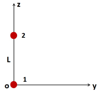
Figure 1: Two gravitationally polarizable subsystems separated from each other by a distance of $L$ in the $z$-axis.

The explicit expressions of the coefficients $A_{i}$ and $B_{i}$ in Eq. (28) are given in appendix A, see Eqs. (40)-(A.1). Since $A_{1}=B_{1}$ and $A_{2}=B_{2}$, it is clear that the criterion for entanglement generation (28) becomes $A_{3}^{2}>0$. That is, entanglement can be generated as long as $A_{3}$, which is dependent on $q_{ij}^{(\alpha)}$ and $\omega L$, is nonzero.

When the polarizations of the two subsystems are the same, for example, when $q^{(\alpha)}_{11}=-q^{(\alpha)}_{22}=|q|$ or $q^{(\alpha)}_{11}=-q^{(\alpha)}_{33}=|q|$ and other components being zero, we plot, in Fig. 2, the coefficient $A_{3}$ as a function of $\omega L$ in the unit of $\Gamma_{0}$, with $\Gamma_{0}=|q|\omega^{5}/\pi$. As $\omega L$ grows, $A_{3}$ oscillates around zero with a decreasing amplitude, and it approaches zero as $\omega L\rightarrow\infty$. That is, when the separation of the two subsystems is infinitely large, they are always separable. Even for finite separations, there are some special values of $\omega L$ that give $A_{3}=0$, so entanglement can not be generated at those separations.

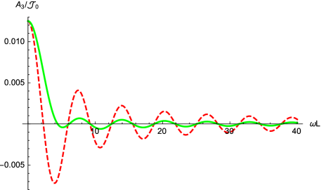
Figure 2: The coefficient $A_{3}$ as a function of $\omega L$. The red dashed line and green solid line correspond to two different polarizations of the subsystems respectively, i.e. $q^{(\alpha)}_{11}=-q^{(\alpha)}_{22}=|q|$ and $q^{(\alpha)}_{11}=-q^{(\alpha)}_{33}=|q|$, with other components being zero.

When the polarizations of the two subsystems are the same, i.e., $q^{(1)}_{ij}=q^{(2)}_{ij}=q_{ij}$, there are no solutions to $F=K=0$ (see Eqs. (A.1)-(A.1)) for any given $L$, i.e., irrespective of the polarization of the two subsystems, the entanglement between the two subsystems with the same polarization can always be generated for a given separation. Therefore, when the polarizations of the two subsystems are the same, they can always get entangled if the separation is finite, except for a series of special values of $\omega L$ which are the zero points of $A_{3}$. Similar conclusions have been drawn in the case of two independent atoms coupled with massless scalar (matter) fields Floreanini . This suggests that there is no difference between spacetime fluctuations and matter fields fluctuations when the entanglement generation is concerned with two subsystems of the same gravitational polarization.

When the polarizations of the two subsystems are different, it can be shown by solving the equations $F=K=0$ that the two subsystems may not get entangled for any given separations when the components of quadrupole moments of the two subsystems satisfy the following conditions simultaneously,

$$q_{33}^{(1)}=0,\ \ \ q_{13}^{(1)}\ q_{13}^{(2)}+q_{23}^{(1)}\ q_{23}^{(2)}=0,\ \ \ 2\ q_{12}^{(1)}\ q_{12}^{(2)}+q_{11}^{(1)}\ (q_{11}^{(2)}-q_{22}^{(2)})=0.$$ (29)

Note that we do not distinguish the two subsystems here, i.e. the superscripts $(1)$ and $(2)$ in the equations above can be exchanged. Recall that $q_{ij}$ is traceless, so $q_{33}^{(\alpha)}=0$ indicates that $q_{11}^{(\alpha)}=-q_{22}^{(\alpha)}$. The components of the quadrupole moment can be interpreted as follows. The diagonal components $q_{11}$, $q_{22}$ and $q_{33}$ respectively represent the contributions to the total mass quadrupole moment from the mass distributed along the $x$ axis, $y$ axis and $z$ axis, and the off-diagonal components $q_{12}$, $q_{13}$ and $q_{23}$ respectively represent the contributions to the total mass quadrupole moment from the mass distributed in the $xoy$, $xoz$ and $yoz$ plane. Therefore, when the mass distributions of the two subsystems induced by quantum gravitational vacuum fluctuations satisfy the condition (29), the two subsystems remain disentangled.

As an example, we consider the case when the two subsystems are only polarizable in the $xoy$ plane, i.e. $q^{(1)}_{3i}=q^{(2)}_{3i}=0$. In this case, we have

$${A_{3}}=\frac{1}{128\pi L^{5}}[F_{1}\sin{(\omega L)}+K_{1}\cos{(\omega L)}\ \omega L],$$ (30)

where

$$F_{1}=4(3-3\omega^{2}L^{2}+\omega^{4}L^{4})q^{(1)}_{12}q^{(2)}_{12}+(9-5\omega^{2}L^{2}+\omega^{4}L^{4})(q^{(1)}_{11}q^{(2)}_{11}+q^{(1)}_{22}q^{(2)}_{22})$$ (31)

$$\qquad\qquad\qquad\qquad\qquad\qquad\qquad\ \ \ \ +(\omega^{2}L^{2}-\omega^{4}L^{4}+3)(q^{(1)}_{11}q^{(2)}_{22}+q^{(1)}_{22}q^{(2)}_{11}),$$

and (32)

$$K_{1}=4(-3+2\omega^{2}L^{2})q^{(1)}_{12}q^{(2)}_{12}+(2\omega^{2}L^{2}-9)(q^{(1)}_{11}q^{(2)}_{11}+q^{(1)}_{22}q^{(2)}_{22})$$

$$\qquad\qquad\qquad\qquad\qquad\qquad\ -(3+2\omega^{2}L^{2})(q^{(1)}_{11}q^{(2)}_{22}+q^{(1)}_{22}q^{(2)}_{11}).$$

It is obvious that when

$$q_{11}^{(1)}\ q_{11}^{(2)}=q_{22}^{(1)}q_{22}^{(2)}=-q_{12}^{(1)}\ q_{12}^{(2)},$$ (33)

$A_{3}$ is always zero, i.e., the entanglement generation cannot happen. Otherwise, the value of ${A_{3}}$ oscillates around zero as $\omega L$ varies with a changing amplitude. This reveals a clear difference between entanglement generation by vacuum fluctuations of massless scalar (matter) fields and that of the spacetime, that is, entanglement generation may never happen for certain polarizations if only spacetime fluctuations are considered.

III.2 Entanglement generation for two gravitationally polarizable subsystems aligned parallel to the boundary

Now we concentrate on the effect of a Dirichlet boundary (recall our comments in the Introduction for gravitational boundaries ) on entanglement generation between two gravitationally polarizable subsystems in a bath of fluctuating gravitational fields. We assume that the Dirichlet boundary is located at $y$=0 in the $xoz$ plane, and the two subsystems separated from each other by a distance $L$ is placed along the $z$ direction at a distance of $y$, see Fig. 3 .

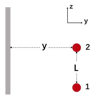
Figure 3: Two independent gravitationally polarizable subsystems are placed along the $z$ direction with a separation $L$, which are at a distance $y$ from a Dirichlet boundary in the $xoz$ plane.

The coefficients $A_{1},~{}A_{2},~{}A_{3}$ and $B_{1},~{}B_{2},~{}B_{3}$ can be calculated from Eq. (23) and Eq. (25) with the Fourier transform of Eq. (43), and the results are lengthy, so we do not give them explicitly here. As before, we will examine when $A^{\prime}_{3}=0$ to determine whether entanglement can be generated or not, since $A^{\prime}_{i}=B^{\prime}_{i}~{}(i=1,2,3)$ still holds in the present circumstances. In this case, the conditions that entanglement cannot be generated for any $L$ are solved as follows

$$q_{12}^{(1)}q_{12}^{(2)}=0,\ \ \ q_{13}^{(1)}q_{13}^{(2)}=0,\ \ \ q_{12}^{(1)}q_{13}^{(2)}=0,\ \ \ q_{22}^{(\alpha)}=q_{33}^{(\alpha)}=q_{23}^{(\alpha)}=0\ (\alpha=1\ \mathrm{or}\ 2),$$ (34)

Now we consider the same example as before, i.e. when the two subsystems are only polarizable in the $xoy$ plane, $q^{(1)}_{3i}=q^{(2)}_{3i}=0$. In this case, we have

$$A^{\prime}_{3}=\frac{1}{128\pi}\left[\frac{F_{1}\sin{(\omega L)}+K_{1}\cos{(\omega L)}\ \omega L}{L^{5}}+\frac{M_{1}\sin{(\omega R)}+N_{1}\cos{(\omega R)}\ \omega R}{R^{9}}\right],$$ (35)

where the explicit expressions of $M_{1}$ and $N_{1}$ are given in appendix (see Eqs. (A.2)-(A.2)). Obviously, if entanglement generation cannot happen for any given $L$ and $y$, the corresponding coefficients satisfy $F_{1}=K_{1}=M_{1}=N_{1}=0$, and then we have

$$q_{12}^{(1)}q_{12}^{(2)}=0,\ \ \ \ q_{11}^{(1)}q_{11}^{(2)}=0.$$ (36)

Comparing the result above with that obtained in the corresponding case without a boundary, we find the condition Eq. (36) is a special case of Eq. (33). That is, if the components of the quadrupole moments satisfy $q_{11}^{(1)}q_{11}^{(2)}=q_{22}^{(1)}q_{22}^{(2)}=-q_{12}^{(1)}q_{12}^{(2)}\neq 0$, the two subsystems can be entangled in the presence of a boundary, while they remain separable in the free space.

III.3 Entanglement creation for two gravitationally polarizable subsystems aligned vertical to the boundary

Now we investigate the case when the alignment of the two gravitationally polarizable subsystems is vertical to the boundary. We assume that the Dirichlet boundary is placed at $z$=0 in the $xoy$ plane and the two subsystems are placed on the $z$-axis with a separation $L$, the distance from the boundary to the nearer subsystem being $z$, see Fig. 4.

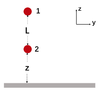
Figure 4: Two independent gravitationally polarizable subsystems are placed on the $z$-axis with a separation $L$. A Dirichlet boundary is located in the $xoy$ plane, and the distance to the closer one is $z$.

Following the same procedures, we find that the conditions that entanglement generation cannot happen for any given $L$ and $z$ are the same with that obtained in the case without a boundary, see Eq. (29). That is, when the quadrupole moments of the two subsystems satisfy certain conditions such that entanglement cannot be generated in the free space, it cannot be generated in the presence of a boundary placed vertically to the alignment of the subsystems either.

IV Summary

In this paper, we have investigated the entanglement generation at the neighborhood of the initial time between two independent gravitationally polarizable two-level subsystems in interaction with a bath of fluctuating quantum gravitational fields in vacuum both with and without a boundary. The partial transposition criterion has been applied to determine whether entanglement can be generated or not at the beginning of evolution. In the free space case, when the polarizations of the two subsystems are the same, the two subsystems can always get entangled as long as the separation is finite. This is similar to what happens when the fluctuations of scalar (matter) fields are considered. When the polarizations of the two subsystems are different, they cannot get entangled in certain circumstances, whatever the separation is. This is in sharp contrast with the case of massless scalar (matter) fields. In the presence of a boundary, we find that in some of the cases where entanglement cannot be generated in a free space, the presence of a boundary placed parallel to the alignment of the subsystems may render the subsystems entangled, but this does not happen for a boundary placed vertically.

Appendix A

The appendix mainly shows some calculations of the coefficients $A_{i}$ and $B_{i}$ in Eq. (28) for the condition of entanglement generation.

A.1 The case in the free Minkowski spacetime

In the free Minkowski spacetime, we assume the two gravitationally polarizable subsystems are placed at the points ${\bf x}_{1}=(0,0,0)$ and ${\bf x}_{2}=(0,0,L)$ respectively, where $L$ denotes the separation between the two subsystems. Straightforward calculations of Eqs. (LABEL:g1) and (19) show that $\mathcal{G}_{ijkl}^{(\alpha\beta)}(-\omega)=0$, and the nonzero components of $\mathcal{G}_{ijkl}^{(\alpha\beta)}(\omega)$ can be written as

$$\mathcal{G}_{ijkl}^{(\alpha\beta)}(\omega)=\frac{\omega^{5}}{\pi}f_{ijkl}^{(\alpha\beta)}(\omega,L).$$ (37)

When $\alpha=\beta$, we have $f_{ijkl}^{(11)}=f_{ijkl}^{(22)}$, where

$$f_{1111}^{(11)}=f_{2222}^{(11)}=f_{3333}^{(11)}=\frac{1}{15},\ \ \ \ \qquad\qquad\qquad f_{1122}^{(11)}=f_{1133}^{(11)}=f_{2233}^{(11)}=-\frac{1}{30},$$

$$f_{1212}^{(11)}=f_{1313}^{(11)}=f_{2323}^{(11)}=\frac{1}{20},\ \ \ \ \qquad\qquad\qquad f_{1122}^{(11)}=f_{2211}^{(11)}=f_{3311}^{(11)}=f_{3322}^{(11)},$$

$$f_{1212}^{(11)}=f_{1221}^{(11)}=f_{1331}^{(11)}=f_{2332}^{(11)}=f_{2112}^{(11)}=f_{3113}^{(11)}=f_{3223}^{(11)}=f_{2121}^{(11)}=f_{3131}^{(11)}=f_{3232}^{(11)},$$ (38)

and when $\alpha\neq\beta$, we have $f_{ijkl}^{(12)}=f_{ijkl}^{(21)}$, where

$$f_{1111}^{(12)}(\omega,L)=\frac{\omega L(-9+2\omega^{2}L^{2})\cos{(\omega L)}+(9-5\omega^{2}L^{2}+\omega^{4}L^{4})\sin{(\omega L)}}{8\omega^{5}L^{5}},$$

$$f_{3333}^{(12)}(\omega,L)=\frac{-3\omega L\cos{(\omega L)}+(3-\omega^{2}L^{2})\sin{(\omega L)}}{\omega^{5}L^{5}},$$

$$f_{1122}^{(12)}(\omega,L)=\frac{-\omega L(3+2\omega^{2}L^{2})\cos{(\omega L)}+(3+\omega^{2}L^{2}-\omega^{4}L^{4})\sin{(\omega L)}}{8\omega^{5}L^{5}},$$

$$f_{1133}^{(12)}(\omega,L)=\frac{3\omega L\cos{(\omega L)}+(-3+\omega^{2}L^{2})\sin{(\omega L)}}{2\omega^{5}L^{5}},$$

$$f_{1212}^{(12)}(\omega,L)=\frac{\omega L(-3+2\omega^{2}L^{2})\cos{(\omega L)}+(3-3\omega^{2}L^{2}+\omega^{4}L^{4})\sin{(\omega L)}}{8\omega^{5}L^{5}},$$

$$f_{1313}^{(12)}(\omega,L)=\frac{\omega L(6-\omega^{2}L^{2})\cos{(\omega L)}+3(-2+\omega^{2}L^{2})\sin{(\omega L)}}{4\omega^{5}L^{5}},$$

$$f_{1111}^{(12)}=f_{2222}^{(12)},\ \ \ \ \ \qquad\qquad\qquad f_{1122}^{(12)}=f_{2211}^{(12)},$$

$$f_{1133}^{(12)}=f_{2233}^{(12)}=f_{3311}^{(12)}=f_{3322}^{(12)},\ \ \ f_{1212}^{(12)}=f_{1221}^{(12)}=f_{2112}^{(12)}=f_{2121}^{(12)},$$

$$f_{1313}^{(12)}=f_{2323}^{(12)}=f_{1331}^{(12)}=f_{2332}^{(12)}=f_{3113}^{(12)}=f_{3223}^{(12)}=f_{3131}^{(12)}=f_{3232}^{(12)}.$$ (39)

The coefficients can be obtained from Eq. (23) and Eq. (25) as

$$A_{1}=B_{1} = \frac{\omega^{5}}{480\pi}\big{\{}(q^{(1)}_{11}-q^{(1)}_{22})^{2}+(q^{(1)}_{11}-q^{(1)}_{33})^{2}+(q^{(1)}_{22}-q^{(1)}_{33})^{2}$$

$$\qquad\quad\qquad\qquad\quad+6[({q^{(1)}_{12}})^{2}+({q^{(1)}_{13}})^{2}+({q^{(1)}_{23}})^{2}]\big{\}},$$

$$A_{2}=B_{2} = \frac{\omega^{5}}{480\pi}\big{\{}(q^{(2)}_{11}-q^{(2)}_{22})^{2}+(q^{(2)}_{11}-q^{(2)}_{33})^{2}+(q^{(2)}_{22}-q^{(2)}_{33})^{2}$$

$$\qquad\quad\qquad\qquad\quad+6[({q^{(2)}_{12}})^{2}+({q^{(2)}_{13}})^{2}+({q^{(2)}_{23}})^{2}]\big{\}},$$

$$A_{3}=B_{3}=\frac{1}{128\pi L^{5}}[F\sin{(\omega L)}+K\cos{(\omega L)}\ \omega L],$$ (40)

with

$$F=(9-5\omega^{2}L^{2}+\omega^{4}L^{4})(q^{(1)}_{11}q^{(2)}_{11}+q^{(1)}_{22}q^{(2)}_{22})+(3+\omega^{2}L^{2}-\omega^{4}L^{4})(q^{(1)}_{11}q^{(2)}_{22}+q^{(1)}_{22}q^{(2)}_{11})$$

$$\qquad\qquad\qquad\ \ \ \ +4(3-3\omega^{2}L^{2}+\omega^{4}L^{4})q^{(1)}_{12}q^{(2)}_{12}+24(-2+\omega^{2}L^{2})(q^{(1)}_{13}q^{(2)}_{13}+q^{(1)}_{23}q^{(2)}_{23})$$

$$\qquad\qquad\qquad\qquad\ +4(\omega^{2}L^{2}-3)(q^{(1)}_{33}q^{(2)}_{11}+q^{(1)}_{11}q^{(2)}_{33}+q^{(1)}_{33}q^{(2)}_{22}+q^{(1)}_{22}q^{(2)}_{33}-2q^{(1)}_{33}q^{(2)}_{33}),$$ (41)

and

$$K=(2\omega^{2}L^{2}-9)(q^{(1)}_{11}q^{(2)}_{11}+q^{(1)}_{22}q^{(2)}_{22})-(3+2\omega^{2}L^{2})(q^{(1)}_{11}q^{(2)}_{22}+q^{(1)}_{22}q^{(2)}_{11})$$

$$\qquad\qquad\ +4(-3+2\omega^{2}L^{2})q^{(1)}_{12}q^{(2)}_{12}-8(-6+\omega^{2}L^{2})(q^{(1)}_{13}q^{(2)}_{13}+q^{(1)}_{23}q^{(2)}_{23})$$

$$\qquad\qquad\qquad\ \ \ +12(q^{(1)}_{33}q^{(2)}_{11}+q^{(1)}_{11}q^{(2)}_{33}+q^{(1)}_{33}q^{(2)}_{22}+q^{(1)}_{22}q^{(2)}_{33}-2q^{(1)}_{33}q^{(2)}_{33}).$$ (42)

A.2 The case for two subsystems aligned parallel to the boundary

As for two gravitationally polarizable subsystems aligned parallel to the boundary, we assume that the boundary is located at $y$=0 in the $xoz$ plane, and the two subsystems separated from each other by a distance $L$ is placed along the $z$ direction at a distance of $y$. With the help of the method of images, the correlation functions can be written in the following form

$$\langle{E_{ij}(t,x_{\alpha})E_{kl}(t^{\prime},x_{\beta})}\rangle_{\mathrm{tot}}={\langle{E_{ij}(t,x_{\alpha})E_{kl}(t^{\prime},x_{\beta})}\rangle}_{\mathrm{free}}-{\langle{E_{ij}(t,x_{\alpha})E_{kl}(t^{\prime},x_{\beta})}\rangle}_{\mathrm{bnd}},$$ (43)

and the coefficients $A^{\prime}_{1},~{}A^{\prime}_{2},~{}A^{\prime}_{3}$ and $B^{\prime}_{1},~{}B^{\prime}_{2},~{}B^{\prime}_{3}$ can be calculated from Eqs. (23)-(25) with the Fourier transform of Eq. (43). The results are lengthy, so we do not give them explicitly here, but $A^{\prime}_{i}=B^{\prime}_{i}~{}(i=1,2,3)$ still holds as it does in the free space.

When the two subsystems are only polarizable in the $xoy$ plane, i.e., $q^{(1)}_{3i}=q^{(2)}_{3i}=0$, we have

$$A^{\prime}_{3}=\frac{1}{128\pi}\left[\frac{F_{1}\sin{(\omega L)}+K_{1}\cos{(\omega L)}\ \omega L}{L^{5}}+\frac{M_{1}\sin{(\omega R)}+N_{1}\cos{(\omega R)}\ \omega R}{R^{9}}\right],$$ (44)

where

$$M_{1}=R^{2}[L^{2}(3-\omega^{2}R^{2}+\omega^{4}R^{4})+8y^{2}(-6+\omega^{2}R^{2}+\omega^{4}R^{4})](q_{11}^{(1)}q_{22}^{(2)}+q_{22}^{(1)}q_{11}^{(2)})$$

$$\qquad\quad\ \ -[9L^{4}-288L^{2}y^{2}+384y^{4}+\omega^{2}(L^{6}-108L^{4}y^{2}-192L^{2}y^{4}+1024y^{6})$$

$$\qquad\ \ \ \ \ \ +\omega^{4}(L^{4}+12L^{2}y^{2}+32y^{4})^{2}]q_{22}^{(1)}q_{22}^{(2)}+R^{4}(5\omega^{2}R^{2}-\omega^{4}R^{4}-9)q_{11}^{(1)}q_{11}^{(2)}$$

$$\qquad\qquad\qquad\qquad\ \ \ \ -4\omega^{2}R^{4}\left[\omega^{2}L^{4}+32\omega^{2}y^{4}+12y^{2}(-1+\omega^{2}L^{2})\right]q_{12}^{(1)}q_{12}^{(2)},$$ (45)

and

$$N_{1}=[6L^{2}y^{2}(\omega^{2}R^{2}-18)-128y^{4}(\omega^{2}R^{2}-3)+L^{4}(9+2\omega^{2}R^{2})]q_{22}^{(1)}q_{22}^{(2)}$$

$$\qquad\qquad\qquad\qquad\ +R^{2}[-3L^{2}+8y^{2}(6+\omega^{2}R^{2})](q_{11}^{(1)}q_{22}^{(2)}+q_{22}^{(1)}q_{11}^{(2)})$$

$$\qquad\qquad\qquad\qquad\quad\ \ \ -R^{4}(2\omega^{2}R^{2}-9)q_{11}^{(1)}q_{11}^{(2)}-48\omega^{2}y^{2}R^{4}q_{12}^{(1)}q_{12}^{(2)}.$$ (46)

References

- (1) B. P. Abbott et al (LIGO and Virgo Collaborations), Phys. Rev. Lett. 116, 061102 (2016).
- (2) B. P. Abbott et al (LIGO and Virgo Collaborations), Phys. Rev. Lett. 116, 241103 (2016).
- (3) B. P. Abbott et al (LIGO and Virgo Collaborations), Phys. Rev. Lett.118, 221101 (2017).
- (4) B. P. Abbott et al (LIGO and Virgo Collaborations), Phys. Rev. Lett. 119, 141101 (2017).
- (5) A. Einstein, Sitzungsber. K. Preuss. Akad. Wiss. 1, 688 (1916).
- (6) L. H. Ford, Phys. Rev. D 51, 1692 (1995).
- (7) H. Yu and L. H. Ford, Phys. Rev. D 60, 084023 (1999).
- (8) H. Yu, N. F. Svaiter, and L. H. Ford, Phys. Rev. D 80, 124019 (2009).
- (9) J. Q. Quach, Phys. Rev. Lett. 114, 081104 (2015).
- (10) L. H. Ford, M. P. Hertzberg, and J. Karouby, Phys. Rev. Lett. 116, 151301 (2016).
- (11) P. Wu, J. Hu and H. Yu, Phys. Lett. B 763, 40 (2016).
- (12) J. Hu and H. Yu, Phys. Lett. B 767, 16 (2017).
- (13) P. Wu, J. Hu and H. Yu, Phys. Rev. D 95, 104057 (2017).
- (14) H. B. G. Casimir, Proc. K. Ned. Akad. Wet. 51, 793 (1948).
- (15) H. B. G. Casimir and D. Polder, Phys. Rev. 73, 360 (1948).
- (16) D. Giulini, E. Joos, C. Kiefer, J. Kupsch, I.-O. Stamatescu, and H. D. Zeh, Decoherence and the Appearance of a Classical World in Quantum Theory (Springer, Berlin, 1996).
- (17) C. Anastopoulos, Phys. Rev. D 54, 1600 (1996).
- (18) B. S. Kay, Class. Quantum Grav. 15, L89 (1998).
- (19) W. L. Power and I. C. Percival, Proc. R. Soc. A 456, 955 (2000).
- (20) P. Kok and U. Yurtsever, Phys. Rev. D 68, 085006 (2003).
- (21) C. H. -T. Wang, R. Bingham, J. Tito Mendonca, Class. Quantum Grav. 23, L59 (2006).
- (22) H.-P. Breuer, E. Göklü and C. Lämmerzahl, Class. Quantum Grav. 26, 105012 (2009).
- (23) C. Anastopoulos and B. L. Hu, Class. Quantum Grav. 30, 165007 (2013).
- (24) M. P. Blencowe, Phys. Rev. Lett. 111, 021302 (2013).
- (25) V. A. De Lorenci and L. H. Ford, Phys. Rev. D 91, 044038 (2015).
- (26) T. Oniga and C. H.-T. Wang, Phys. Rev. D 93, 044027 (2016).
- (27) A. Bassi, A. Großardt, and H. Ulbricht, Class. Quantum Grav. 34, 193002 (2017).
- (28) A. Valentini, Phys. Lett. A 153, 321 (1991).
- (29) L. Jakobczyk, J. Phys. A 35, 6383 (2002).
- (30) B. Reznik, Found. Phys. 33, 167 (2003).
- (31) B. Reznik, A. Retzker, and J. Silman, Phys. Rev. A 71, 042104 (2005).
- (32) A. Pozas-Kerstjens and E. Martn-Martnez, Phys. Rev. D 94, 064074 (2016).
- (33) F. Benatti and R. Floreanini, Phys. Rev. A 70, 012112 (2004).
- (34) M. B. Plenio, S. F. Huelga, A. Beige, and P. L. Knight, Phys. Rev. A 59, 2468 (1999).
- (35) D. Braun, Phys. Rev. Lett. 89, 277901 (2002).
- (36) M. S. Kim, J. Lee, D. Ahn, and P. L. Knight, Phys. Rev. A 65, 040101(2002).
- (37) S. Schneider and G. J. Milburn, Phys. Rev. A 65, 042107 (2002).
- (38) A. M. Basharov, J. Exp. Theor. Phys. 94, 1070 (2002).
- (39) F. Benatti, R. Floreanini, and M. Piani, Phys. Rev. Lett. 91, 070402 (2003).
- (40) F. Benatti and R. Floreanini, J. Opt. B: Quantum Semiclassical Opt. 7, S429 (2005).
- (41) J. Zhang and H. Yu, Phys. Rev. A 75, 012101 (2007).
- (42) J. Zhang and H. Yu, Phys. Rev. D 75, 104014 (2007).
- (43) J. Hu and H. Yu, Phys. Rev. A 91, 012327 (2015).
- (44) Y. Yang, J. Hu and H. Yu, Phys. Rev. A 94, 032337 (2016).
- (45) C. Kiefer, C. Weber, Ann. Phys. (Leipz.) 14, 253 (2005).
- (46) S. J. Minter, K. Wegter-McNelly, and R. Y. Chiao, Physica 42E, 234 (2010).
- (47) R. Y. Chiao, J. S. Sharping, L. A. Martinez, B. S. Kang, A. Castelli, N. Inan, and J. J. Thompson, arXiv:1712.08680.
- (48) W. B. Campbell and T. A. Morgan, Am. J. Phys. 44, 356 (1976).
- (49) A. Matte, Can. J. Math. 5, 1 (1953).
- (50) W. Campbell and T. Morgan, Physica (Amsterdam) 53, 264 (1971).
- (51) P. Szekeres, Ann. Phys. (N.Y.) 64, 599 (1971).
- (52) R. Maartens and B. A. Bassett, Classical Quant. Grav. 15, 705 (1998).
- (53) M. L. Ruggiero and A. Tartaglia, Nuovo Cimento B 117, 743 (2002).
- (54) J. Ramos, M. de Montigny, and F. Khanna, Gen. Relativ. Gravit. 42, 2403 (2010).
- (55) R. Ingraham, Gen. Relativ. Gravit. 29, 117 (1997).
- (56) V. Gorini, A. Kossakowski, and E. C. G. Surdarshan, J. Math. Phys. 17, 821 (1976).
- (57) G. Lindblad, Commun. Math. Phys. 48, 119 (1976).
- (58) A. Peres, Phys. Rev. Lett. 77, 1413 (1996).
- (59) M. Horodecki, P. Horodecki, and R. Horodecki, Phys. Lett. A 223, 1 (1996).