Learning Transferable Adversarial Examples via Ghost Networks

Abstract

Recent development of adversarial attacks has proven that ensemble-based methods outperform traditional, non-ensemble ones in black-box attack. However, as it is computationally prohibitive to acquire a family of diverse models, these methods achieve inferior performance constrained by the limited number of models to be ensembled.

In this paper, we propose Ghost Networks to improve the transferability of adversarial examples. The critical principle of ghost networks is to apply feature-level perturbations to an existing model to potentially create a huge set of diverse models. After that, models are subsequently fused by longitudinal ensemble. Extensive experimental results suggest that the number of networks is essential for improving the transferability of adversarial examples, but it is less necessary to independently train different networks and ensemble them in an intensive aggregation way. Instead, our work can be used as a computationally cheap and easily applied plug-in to improve adversarial approaches both in single-model and multi-model attack, compatible with residual and non-residual networks. By reproducing the NeurIPS 2017 adversarial competition, our method outperforms the No.1 attack submission by a large margin, demonstrating its effectiveness and efficiency. Code is available at https://github.com/LiYingwei/ghost-network.

Introduction

In recent years, Convolutional Neural Networks (CNNs) have greatly advanced performance in various vision tasks, including image recognition (?; ?; ?), object detection (?; ?), and semantic segmentation (?), etc.. However, it has been observed (?; ?) that adding human imperceptible perturbations to input image can cause CNNs to make incorrect predictions even if the original image can be correctly classified. These intentionally generated images are usually called adversarial examples (?; ?; ?). Besides image classification, adversarial examples also exist on other tasks (?; ?; ?; ?; ?).

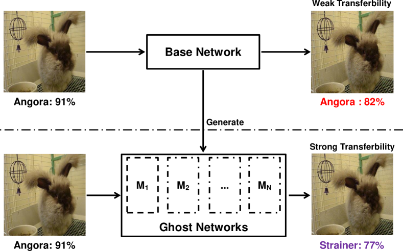
Figure 1: An illustration of the capacity of the proposed ghost networks in learning transferable adversarial examples. The base model is ResNet-50, which is used to generate adversarial examples and to generate ghost networks. The evaluation is done on Inception v3.

Two attack settings are later developed, i.e., white-box attack and black-box attack. In white-box attack, attackers can access the model (?; ?). By contrast, in black-box attack, attackers cannot access the target model. A typical solution is to generate adversarial examples with strong transferability (transferable adversarial examples).

The transferability of adversarial examples refers to the property that the same input can successfully attack different models (?). Taking advantage of the transferability, (?) develop a black-box (attackers cannot access the target model) attack system by attacking a substitute model. (?) suggest attacking an ensemble of substitute models could improve transferability. Based on (?) and I-FGSM, several methods are developed to further improve the transferability by smoothing gradient (?; ?). In this work, we focus on learning transferable adversarial examples for black-box attack.

Focusing on the transferability, many attempts have been made, such as attacking a substitute model (?) or an ensemble of multiple substitute models (?; ?; ?). In particular, the ensemble-based attacks obtain much better performance than the non-ensemble ones, and thus have attracted many attentions. Almost all top-ranked entries in competitions use ensemble-based attacks (?).

However, the ensemble-based attacks suffer from expensive computational overhead, making it difficult to generate transferable adversarial examples efficiently. First, in order to acquire good (i.e., low test error) and diverse (i.e., converge at different local minima) models, people usually independently train them from scratch. Second, to leverage their complementarity, existing methods adopt an intensive aggregation way to fuse the outputs of those networks (e.g., logits). Consequently, attacking methods in competitions (like ? (?)) generally ensemble at most only ten networks restricted by the high computational cost. However, efficiently attacking a huge ensemble of models is critical.

How to improve the transferability of adversarial examples without additional cost remains a challenging task. ?; ?; ? (?; ?; ?) suggest that re-training networks can achieve high transferability. ?; ?; ? (?; ?; ?) propose query-based methods to attack black-box model without substitute models, which require extensive information from the target model. In conclusion, acquiring and integrating information from various models to approximate the target model is the key to achieving better transferability. However, most works are inefficient and inadequate to learn adversarial examples with strong transferability. Our work addresses this issue.

In this paper, we propose a highly efficient alternative called Ghost Networks to address this issue. As shown in Fig. 1, the basic principle is to generate a vast number of virtual models built on a base network (a network trained from scratch). The word “virtual” means that these networks are not stored or trained (therefore termed as ghost networks). Instead, they are generated by imposing erosion on certain intermediate structures of the base network on-the-fly. However, with an increasing number of models we have, a standard ensemble (?) would be problematic owing to its complexity. Accordingly, we propose Longitudinal Ensemble, a specific fusion method for ghost networks, which conducts an implicit ensemble during attack iterations. Consequently, adversarial examples can be easily generated without sacrificing computational efficiency.

To summarize, the contributions of our work are divided into three folds: 1) Our work is the first one to explore network erosion to learn transferable adversarial examples, not solely relying on multi-network ensemble. 2) We observe that the number of different networks used for ensemble (intrinsic networks) is essential for transferability. However, it is less necessary to train different models independently. Ghost networks can be a competitive alternative with extremely low complexity. 3) Ghost network is generic. Seemingly an ensemble method for multi-model attacks, it can also be applied to single-model attacks where only one trained model is accessible. Furthermore, it is also compatible with various network structures, attack methods, and adversarial settings.

Extensive experimental results demonstrate our method improves the transferability of adversarial examples, acting as a computationally cheap plug-in. In particular, by reproducing NeurIPS 2017 adversarial competition (?), our work outperforms the No.1 attack submission by a large margin, demonstrating its effectiveness and efficiency.

Backgrounds

This section introduces two iterative-based methods, Iterative Fast Gradient Sign Method (I-FGSM) (?) and Momentum I-FGSM (MI-FGSM) (?).

I-FGSM was proposed by Kurakin et al. (?), and learns the adversarial example $I^{\text{adv}}$ by

$$\begin{split}&I_{0}^{\text{adv}}=I,\\ &I_{n+1}^{\text{adv}}=\text{Clip}_{I}^{\epsilon}\{I_{n}^{\text{adv}}+\alpha\text{sign}\left(\nabla_{I}L(I_{n}^{\text{adv}},y^{\text{true}};\theta)\right)\},\end{split}$$ (1)

where $L$ is the loss function of a network with parameter $\theta$. $\text{Clip}_{I}^{\epsilon}$ is the clip function which ensures the generated adversarial example is within the $\epsilon$-ball of the original image $I$ with ground-truth label $y^{\text{true}}$. $n$ is the iteration number and $\alpha$ is the step size.

MI-FGSM was proposed by Dong et al. (?), and integrates the momentum term into the attack process to stabilize the update directions and escape from poor local maxima. At the $n$-th iteration, the accumulated gradient $g_{n+1}$ is calculated by:

$$g_{n+1}=\mu\cdot g_{n}+\frac{\nabla_{I}L(I_{n}^{\text{adv}},y^{\text{true}};\theta)}{||\nabla_{I}L(I_{n}^{\text{adv}},y^{\text{true}};\theta)||_{1}},$$ (2)

where $\mu$ is the decay factor of the momentum term. The sign of the accumulated gradient $g_{n+1}$ is then used to generate the adversarial example, by

$$I_{n+1}^{\text{adv}}=\text{Clip}_{I}^{\epsilon}\{I_{n}^{\text{adv}}+\alpha\text{sign}(g_{n+1})\}.$$ (3)

Ghost Networks

The goal of this work is to learn transferable adversarial examples. Given a clean image $I$, we want to find an adversarial example $I^{\text{adv}}=I+r$, which is still visually similar to $I$ after adding adversarial noise $\|r\|_{\infty}<\epsilon$ but fools the classifier.

Without additional cost, we generate a huge number of ghost networks from a single trained model for later attack by applying feature-level perturbations to non-residual and residual based networks in the next two subsections respectively. Then we present an efficient customized fusion method, longitudinal ensemble, leading to ensemble a huge amount of ghost networks possible.

Dropout Erosion

Revisit Dropout. Dropout (?) is one of the most popular techniques in deep learning. By randomly dropping out units from the model during training phase, dropout can prevent deep neural networks from overfitting. Let $x_{l}$ be the activation in the $l^{\text{th}}$ layer, at training time, the output $y_{l}$ after the dropout layer can be mathematically defined as

$$\begin{split}&y_{l}=r_{l}*x_{l},\\ &r_{l}\sim\text{Bernoulli}(p),\end{split}$$ (4)

where $*$ denotes an element-wise product and $\text{Bernoulli}(p)$ denotes the Bernoulli distribution with the probability $p$ of elements in $r_{l}$ being $1$. At the test time, units in $x_{l}$ are always present, thus to keep the output $y_{l}$ the same as the expected output at the training time, $y_{l}$ is set to be $px_{l}$.

Perturb Dropout. Dropout provides an efficient way of approximately combining different neural network architectures and thereby prevents overfitting. Inspired by this, we propose to generate ghost networks by inserting the dropout layer. To make ghost networks as diverse as possible, we densely apply dropout to every block throughout the base network, rather than simply enable default dropout layers (?). From our preliminary experiments, the latter cannot provide transferability. Therefore, diversity is not limited to high-level features but applied to all feature levels.

Let $f_{l}$ be the function between the $i^{\text{th}}$ and $(i+1)^{\text{th}}$ layer, i.e., $x_{l+1}=f_{l}(x_{l})$, then the output $g_{l}(x_{l})$ after applying dropout erosion is

$$\begin{split}&g_{l}(x_{l})=f_{l}\Big{(}\frac{r_{l}*x_{l}}{1-\Lambda}\Big{)},\\ &r_{l}\sim\text{Bernoulli}(1-\Lambda),\end{split}$$ (5)

where $\Lambda=1-p$, and $p$ has the same meaning as in Eq. (4), indicating the probability that $x_{l}$ is preserved. To keep the expected input of $f_{l}(\cdot)$ consistent after erosion, the activation of $x_{l}$ should be divided by $1-\Lambda$.

During the inference, the output feature after $(L-1)$-th dropout layer ($L>l$) is

$$x_{L}=g_{L-1}\circ g_{L-2}\circ g_{L-3}\circ\cdots\circ g_{l}(x_{l}),$$ (6)

where $\circ$ denotes composite function, i.e., $g\circ f(x)=g\left(f(x)\right)$.

By combining Eq. (5) and Eq. (6), we observe that when $\Lambda=0$ (means $p=1$), all elements in $r_{l}$ equal to $1$. In this case, we do not impose any perturbations to the base network. When $\Lambda$ gradually increases to $1$ ($p$ decreases to $0$), the ratio of elements dropped out is $\Lambda$. In other words, $(1-\Lambda)$ of elements can be back-propagated. Hence, larger $\Lambda$ implies a heavier erosion on the base network. Therefore, we define $\Lambda$ to be the magnitude of erosion.

When perturbing dropout layers, the gradient in back-propagation can be written as

$$\frac{\partial x_{L}}{\partial x_{l}}=\prod_{l\leq i<L}\left(\frac{r_{i}}{1-\Lambda}*\frac{\partial}{\partial x_{i}}f_{i}\Big{(}\frac{r_{i}*x_{i}}{1-\Lambda}\Big{)}\right).$$ (7)

As shown in Eq. (7), deeper networks with larger $L$ are influenced more easily according to the product rule. We will experimentally analyze the impact of $\Lambda$ in the experiments part.

Generate Ghost Network. The generation of ghost networks via perturbing dropout layer proceeds in three steps: 1) randomly sample a parameter set from the Bernoulli distribution $r=\{r_{1},r_{2}...,r_{l},...,r_{L}\}$; 2) apply Eq. (5) to the base network with the parameter set $r$ and get the perturbed network; 3) repeat step 1) and step 2) to independently sample $r$ for $N$ times and obtain a pool of ghost networks $M=\{M_{1},M_{2},...,M_{N}\}$ which can be used for adversarial attacks.

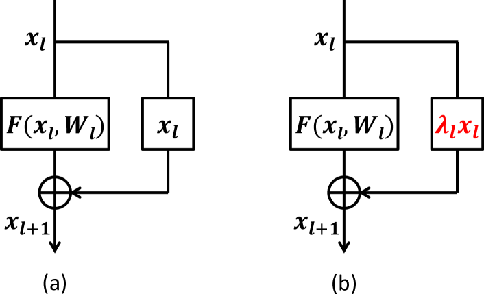
Figure 2: An illustration of skip connection (a, Eq. (8)) and skip connection erosion (b, Eq. (9)).

Skip Connection Erosion

Revisit Skip Connection. ? (?) propose skip connections in CNNs, which makes it feasible to train very deep neural networks. The residual block is defined by

$$x_{l+1}=h(x_{l})+F(x_{l},W_{l}),$$ (8)

where $x_{l}$ and $x_{l+1}$ are the input and output to the $l$-th residual block with the weights $W_{l}$. $F(\cdot)$ denotes the residual function. As suggested in ? (?), it is crucial to uses the identity skip connection, i.e., $h(x_{l})=x_{l}$, to facilitate the residual learning process, otherwise the network may not converge to a good local minima.

Perturb Skip Connection. Following the principle of skip connection, we propose to perturb skip connections to generate ghost networks.

Specifically, the network weights are first learned using identity skip connections, then switched to the randomized skip connection (see Fig. 2). To this end, we apply randomized modulating scalar $\lambda_{l}$ to the $l$-th residual block by

$$x_{l+1}=\lambda_{l}x_{l}+F(x_{l},W_{l}),$$ (9)

where $\lambda_{l}$ is drawn from the uniform distribution $U[1-\Lambda,1+\Lambda]$. One may have observed several similar formulations on skip connection to improve the classification performance, e.g., the gated inference in ? (?) and lesion study in ? (?). However, our work focuses on attacking the model with a randomized perturbation on skip connection, i.e., the model is not trained via Eq. (9).

During inference, the output after $(L-1)$th layer is

$$x_{L}=(\prod_{i=l}^{L-1}\lambda_{i})x_{l}+\sum_{i=l}^{L-1}(\prod_{j=i+1}^{L-1}\lambda_{j})F(x_{i},W_{i}).$$ (10)

The gradient in back-propagation is then written as

$$\frac{\partial x_{L}}{\partial x_{l}}=(\prod_{i=l}^{L-1}\lambda_{i})+\sum_{i=l}^{L-1}(\prod_{j=i+1}^{L-1}\lambda_{j})\frac{\partial F(x_{i},W_{i})}{\partial{x_{l}}}.$$ (11)

Similar to the analysis of dropout erosion, we conclude from Eq. (10) and Eq. (11) that a larger $\Lambda$ will have a greater influence on the base network and deeper networks are easily influenced.

Generate Ghost Network. The generation of ghost networks via perturbing skip connections is similar to that via perturbing the dropout layer. The only difference is we need to sample a set of modulating scalars $\lambda=\{\lambda_{1},\lambda_{2},...,\lambda_{L}\}$ from the uniform distribution for each skip connection.

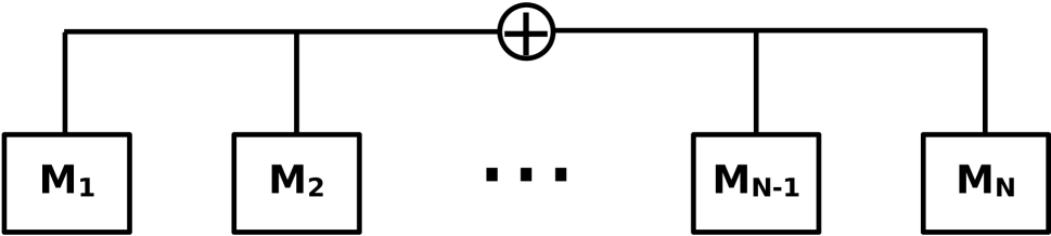
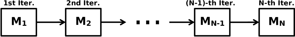
Figure 3: The illustration of the standard ensemble (a) and the proposed longitudinal ensemble (b).

Longitudinal Ensemble

The existing iteration-based ensemble-attack approach (?) require averaging the outputs (e.g., logits, classification probabilities, losses) of different networks. However, such a standard ensemble is too costly and inefficient for us because we can readily obtain a huge candidate pool of qualified neural models by using Ghost Networks.

To remedy this, we propose longitudinal ensemble, a specific fusion method for Ghost Networks, which constructs an implicit ensemble of the ghost networks by randomizing the perturbations during iterations of adversarial attack (e.g., I-FGSM (?) and MI-FGSM (?)). Suppose we have a base model $B$, which can generate a pool of networks $M=\{M_{1},M_{2},...,M_{N}\}$, where $N$ is the model number. The critical step of longitudinal ensemble is that at the $j$-th iteration, we attack the ghost network $M_{j}$ only. In comparison, for each iteration, standard ensemble methods require fusing gradients of all the models in the model pool $M$, leading to high computational cost. We illustrate the difference between the standard ensemble and the longitudinal ensemble method in Fig. 3.

The longitudinal ensemble shares the same prior as ? (?) that if an adversarial example is generated by attacking multiple networks, it is more likely to transfer to other networks. However, longitudinal ensemble method removes duplicated computations by sampling only one model from the pool rather than using all models in each iteration.

There are three noteworthy comments here. First, ghost networks are never stored or trained, reducing both additional time and space cost. Second, it is evident from Fig. 3 that attackers can combine ? (?) and longitudinal ensemble of ghost networks. Finally, it is easy to extend longitudinal ensemble to multi-model attack by treating each base model as a branch (details are in experimental evaluations).

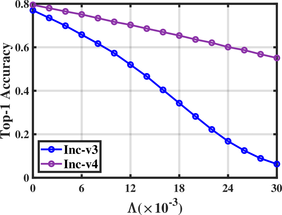
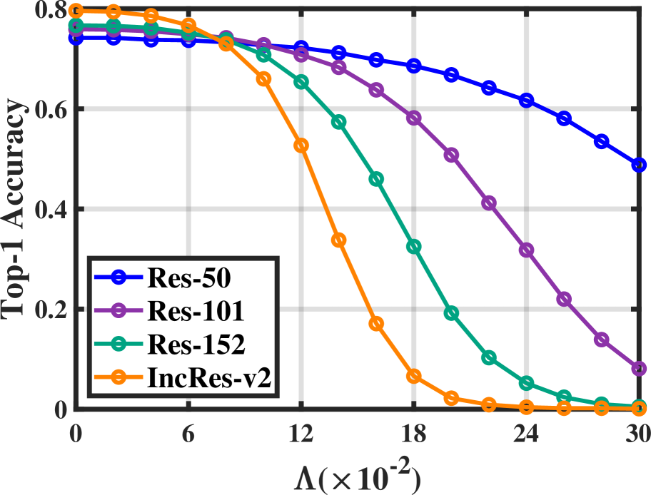
Figure 4: The top-1 accuracy of dropout erosion (a) and skip connection erosion (b) with different magnitude $\Lambda$ .

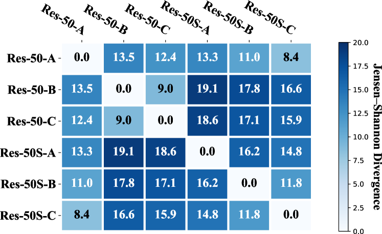
Figure 5: The illustration of the mean diversity $(\times 10^{-2})$ of any pair of networks over the ILSVRC 2012 validation set.The higher value indicates larger diversity.

Methods	Settings				Res-50		Res-101		Res-152		IncRes-v2		Inc-v3		Inc-v4		CC
	MT	#S	#L	#I	I-	MI-	I-	MI-	I-	MI-	I-	MI-	I-	MI-	I-	MI-
Exp. S1	$B$	1	1	1	16.3	29.4	17.8	31.3	16.7	29.6	8.3	20.0	5.3	13.7	7.3	18.4	1
Exp. S2	$M$	1	1	1	8.4	17.4	6.1	19.9	6.4	17.9	5.7	15.2	1.7	5.6	1.9	7.2	1
Exp. S3	$M$	1	10	10	23.4	39.4	23.7	40.1	21.1	38.0	11.2	26.8	6.3	17.6	10.0	22.4	1
Exp. S4	$M$	10	1	10	28.8	44.5	29.9	43.2	25.6	41.9	13.1	30.4	6.3	17.9	9.3	25.6	10
Exp. S5	$M$	10	10	100	35.9	50.6	35.9	51.4	60.1	64.9	14.6	33.3	12.3	28.3	19.4	37.4	10

Table 1: The average black-box attack rate (%) comparison of different methods over two iterative methods, “I-” for I-FGSM and “MI-” for MI-FGSM. MT denotes model type (either $B$ for the base model, or $M$ for ghost networks), #I denotes the number of intrinsic models, and #S (or #L) denotes the number of models for standard (or longitudinal) ensemble in each iteration (branch). CC denotes the computational cost, which is a relative value and we set the CC of Exp. S1 as $1$. We marked all highest attack success rate under the same CC in boldface.

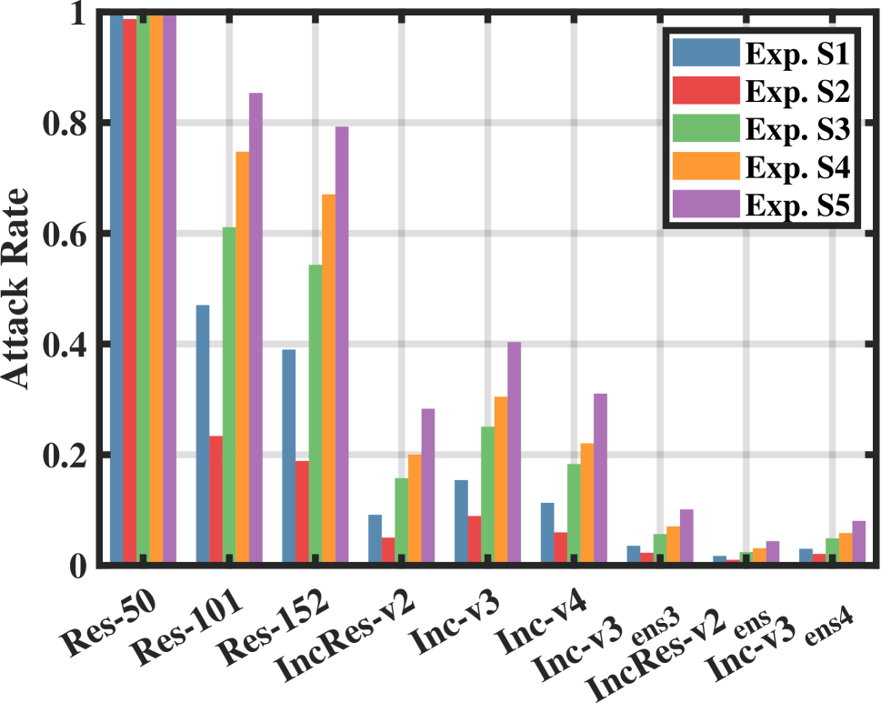
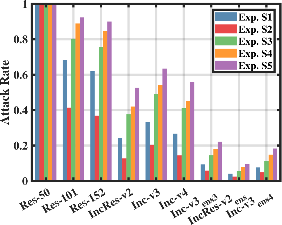
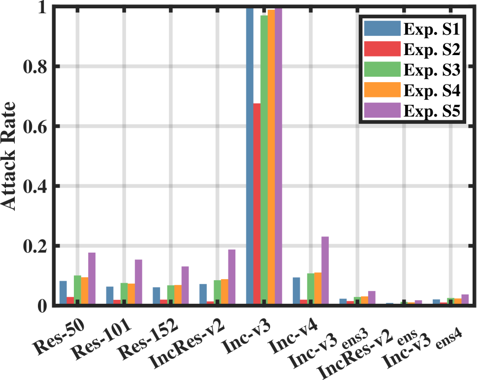
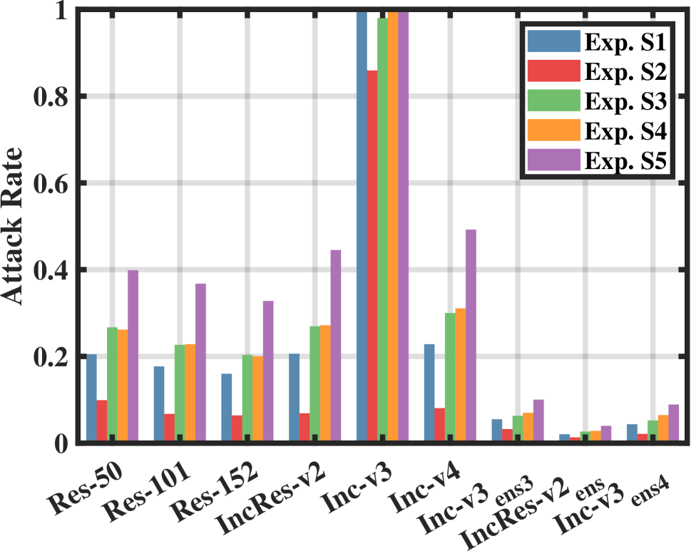
Figure 6: The attack rate (%) comparison when attacking Res-50 (a)(b) and Inc-v3 (c)(d) with I-FGSM (a)(c) and MI-FGSM (b)(d).

Methods	Settings					Attack Rate		CC
	MT	#B	#S	#L	#I	I-	MI-
Exp. M1	$B$	1	1	1	1	25.5	37.2	1
Exp. M2	$B$	3	3	1	3	33.6	46.8	3
Exp. M3	$M$	1	3	1	3	28.9	37.2	3
Exp. M4	$M$	3	3	1	3	26.3	40.8	3
Exp. M5	$M$	1	3	10	30	38.3	52.5	3
Exp. M6	$M$	3	3	10	30	41.1	54.3	3

Table 2: The comparison of attack rate ($\%$) of multi-model attack. “I-”, “MI-”, MT, #S, #L, #I and CC have the same meaning as in Table 1. #B denotes the number of base models. We test on the $9$ networks described in the Experimental Setup section and report the average performances.

Experiments

In this section, we give a comprehensive experimental evaluation of the proposed Ghost Networks. In order to distinguish models trained from scratch and the ghost networks we generate, we call the former one the base network or base model in the rest of this paper. We release source code and provide additional experimental results in https://github.com/LiYingwei/ghost-network.

Experimental Setup

Base Networks. $9$ base models are used in our experiments, including $6$ normally trained models, i.e., Resnet v2-{50, 101, 152} (Res-{50, 101, 152}) (?), Inception v3 (Inc-v3) (?), Inception v4 (Inc-v4) and Inception Resnet v2 (IncRes-v2) (?), and $3$ adversarially-trained models (?) , i.e., Inc-v3_ens3, Inc-v3_ens4 and IncRes-v2_ens.

Datasets. Because it is less meaningful to attack images that are originally misclassified, following ? (?), we select $5000$ images from the ILSVRC 2012 validation set, which can be correctly classified by all the $9$ base models.

Attacking Methods. We employ two iteration-based attack methods mentioned in the Backgrounds section to evaluate the adversarial robustness, i.e., I-FGSM and MI-FGSM.

Parameter Specification. If not specified otherwise, we follow the default settings in ? (?), i.e., step size $\alpha=1$ and the total iteration number $N=\min(\epsilon+4,1.25\epsilon)$. We set the maximum perturbation $\epsilon=8$ (the iteration number $N=10$ in this case). For the momentum term, the decay factor $\mu$ is set to be $1$ as in ? (?).

Analysis of Ghost Networks

In order to learn adversarial examples with good transferability, there are generally two requirements for the intrinsic models. First, each model should have a low test error. Second, different models should be diverse (i.e., converge at different local minima). To show the generated ghost networks are qualified for adversarial attack, we experiment with the whole ILSVRC 2012 validation set.

Descriptive Capacity. In order to quantitatively measure the descriptive capacity of the generated ghost networks, we plot the relationship between the magnitude of erosion $\Lambda$ and top-1 classification accuracy.

We apply dropout erosion to non-residual networks (Inc-v3 and Inc-v4) and skip connection erosion to residual networks (Res-50, Res-101, Res-152 and IncRes-v2). Fig. 4 (a) and (b) present the accuracy curves of the dropout erosion and skip connection erosion, respectively.

The classification accuracies of different models are negatively correlated to the magnitude of erosion $\Lambda$ as expected. By choosing the performance drop approximately equal to 10% as a threshold, we can determine the value of $\Lambda$ individually for each network. Specifically, in our following experiments, $\Lambda$s are $0.006$, $0.012$, $0.22$, $0.16$, $0.12$ and $0.08$ for Inc-v3, Inc-v4, Res-50, Res-101, Res-152, and IncRes-v2 respectively unless otherwise specified. As emphasized throughout this paper, it is extremely cheap to generate a huge number of ghost networks that still preserve relative low error rates.

Model Diversity. To measure diversity, we use Res-50 as the backbone model. We denote the base Res-50 described in the Experimental Setup section as Res-50-A, and independently train two additional models with the same architecture, denoted by Res-50-B and Res-50-C. Meanwhile, we apply skip connection erosion to Res-50-A, then obtain three ghost networks denoted as Res-50S-A, Res-50S-B, and Res-50S-C, respectively.

We employ the Jensen-Shannon Divergence (JSD) as the evaluation metric for model diversity. Concretely, we compute the pairwise similarity of the output probability distribution (i.e., the predictions after softmax layer) for each pair of networks as in ? (?). Given any image, let $X$ and $Y$ denote the softmax outputs of two networks, then

$$\text{JSD}(X||Y)=\frac{1}{2}D(X\|Z)+\frac{1}{2}D(Y\|Z),$$ (12)

where $Z$ is the average of $X$ and $Y$, i.e., $Z=(X+Y)/2$. $D(\cdot)$ is the Kullback-Leibler divergence.

In Fig. 5, we report the averaged JSD for all pairs of networks over the ILSVRC 2012 validation set. As can be drawn, the diversity among ghost networks is comparable or even more significant than independently trained networks.

Based on the analysis of descriptive capacity and model diversity, we can see that generated ghost networks can provide accurate yet diverse descriptions of the data manifold, which is beneficial to learn transferable adversarial examples as we will experimentally prove below.

Methods	Hold-out						Ensemble
	-Res-50	-Res-101	-Res-152	-IncRes-v2	-Inc-v3	-Inc-v4	Inc-v3ens3	Inc-v3ens4	IncRes-v2ens
I-FGSM	71.08	71.16	67.92	46.60	59.98	50.86	15.94	8.54	13.72
I-FGSM + ours	80.22	79.80	77.02	60.20	73.18	67.84	25.80	13.56	21.42
MI-FGSM	79.32	79.14	77.26	64.24	72.22	66.64	29.98	16.66	26.16
MI-FGSM + ours	87.14	86.14	84.64	74.18	82.06	79.18	39.56	21.24	32.68

Table 3: The attack rate (%) comparison of multi-model attack. “Ensemble” means attack all $6$ naturally-trained models. “Hold-out” means attack $5$ out of $6$ models. The sign “-” indicates the name of the hold-out model.

Methods	Black-box Attack				White-box Attack
	TsAIL	iyswim	Anil Thomas	Average	Inc-v3_adv	IncRes-v2_ens	Inc-v3	Average
No.1 Submission	13.60	43.20	43.90	33.57	94.40	93.00	97.30	94.90
No.1 Submission+ours	14.80	52.28	51.68	39.59	97.62	96.00	95.48	96.37

Table 4: The attack rate (%) comparison in the NeurIPS 2017 Adversarial Challenge.

Single-model Attack

Firstly, we evaluate the ghost networks in single-model attack, where attackers can only access one base model $B$ trained from scratch. To demonstrate the effectiveness of our method, we design five experimental comparisons. The setting, black-box attack success rate, and properties are shown in Table 1. The difference among five experiments is the type of model to attack, the number of models ensembled by standard ensemble (?) in each iteration, and the number of models ensembled by longitudinal ensemble in each branch of the standard ensemble. For example, Exp. S5 combines two ensemble methods, that is, we do a standard ensemble of $10$ models for each iteration of attack and a longitudinal ensemble of $10$ models. Therefore, in Exp. S5, the intrinsic number of models is $100$.

We attack $6$ normally-trained networks and test on all the $9$ networks (include $3$ adversarially-trained networks). The attack rate is shown in Table 1. To save space, we report the average attack rate for black-box models. Individual cases are shown in Fig. 6.

As can be drawn from Table 1, a single ghost network is worse than the base network (Exp. S2 vs. Exp. S1), because the descriptive power of ghost networks is inferior to base networks. However, by leveraging the longitudinal ensemble, our work achieves a much higher attack rate in most settings (Exp. S3 vs. Exp. S1). This observation firmly demonstrates the effectiveness of ghost networks in learning transferable adversarial examples. It should be mentioned that the computational cost of Exp. S3 almost remains the same as Exp. S1 for two reasons. First, the $10$ ghost networks used in Exp. S3 are not trained but eroded from the base model and used on-the-fly. Second, multiple ghost networks are fused via the longitudinal ensemble, instead of the standard ensemble method in ? (?).

The proposed ghost networks can also be fused via the standard ensemble method, as shown in Exp. S4. In this case, we achieve a higher attack rate at the sacrifice of computational efficiency. This observation inspires us to combine the standard ensemble and the longitudinal ensemble as shown in Exp. S5. As we can see, Exp. S5 consistently beats all the compared methods in all the black-box settings. Of course, Exp. S5 is as computational expensive as Exp. S4. However, the additional computational overhead stems from the standard ensemble rather than longitudinal ensemble.

Note that in all the experiments presented in Table 1, we use only one individual base model. Even in the case of Exp. S3, all the to-be-fused models are ghost networks. However, the generated ghost networks are never stored or trained, meaning no extra space complexity. Therefore, the benefit of ghost networks is obvious. Especially when comparing Exp. S5 and Exp. S1, ghost networks can achieve a substantial improvement in black-box attack.

Based on the experimental results above, we arrive at a similar conclusion as ? (?): the number of intrinsic models is essential to improve the transferability of adversarial examples. However, a different conclusion is that it is less necessary to train different models independently. Instead, ghost networks is a computationally cheap alternative enabling good performance. When the number of intrinsic models increases, the attack rate will increase. We will further exploit this phenomenon in multi-model attack.

In Fig. 6, we select two base models, i.e., Res-50, and Inc-v3, to attack and present their performances when testing on all the $9$ base models. It is easy to observe the improvement of transferability by adopting ghost networks.

Multi-model Attack

We evaluate ghost networks in multi-model setting, where attackers have access to multiple base models.

Same Architecture and Different Parameters

We firstly evaluate a simple setting of multi-model attack, where base models share the same network architecture but have different weights. The same three Res-50 models as in the Analysis of Ghost Networks section are used. The settings of $6$ experiments are shown in Table 2. Besides a new parameter #B (the number of trained-from-scratch models), others are the same as the single model attack setting. When #B is $1$, we will use Res-50-A as the only one base model, and settings are the same as single-model attack. When #B is $3$, #S is always $3$, and each branch of the standard ensemble is assigned to a different base model. In Exp. M4 and Exp. M6, the ghost network(s) in each standard ensemble branch will be generated by the base model assigned to that branch.

The adversarial examples generated by each method are used to test on all the $9$ models. We report the average attack rates in Table 2. It is easy to understand that Exp. M2 performs better than Exp. M1, Exp. M3, and Exp. M4 as it has three independently trained models. However, by comparing Exp. M5 with Exp. M2, we observe a significant improvement of attack rate. For example, By using MI-FGSM as the attack method, Exp. M5 beats Exp. M2 by $6.70$. Although Exp. M5 only has $1$ base model and Exp. M2 has $3$, Exp. M5 actually fuses $30$ intrinsic models. Such a result further supports our previous claim that the number of intrinsic models is essential, but it is less necessary to obtain them by training from scratch independently. Similarly, Exp. M6 yields the best performance as it has $3$ independently trained models and $30$ intrinsic models.

Different Architectures

Besides the baseline comparison above, we then evaluate ghost networks in the multi-model setting following ? (?). We attack an ensemble of $5$ out of $6$ normally-trained models in this experiment, then test the hold-out network (black-box setting). We also attack an ensemble of $6$ normally-trained models and test on the $3$ adversarially-trained networks to evaluate the transferability of the generated adversarial examples in black-box attack.

The results are summarized in Table 3, the performances in black-box attack are significantly improved. For example, when holding out Res-50, our method improves the performance of I-FGSM from $71.08$ to $80.22$, and that of MI-FGSM from $79.32$ to $87.14$. When testing on the three adversarially-trained networks, the improvement is more notable. These results further testify the ability of ghost networks to learn transferable adversarial examples.

NeurIPS 2017 Adversarial Challenge

Finally, we evaluate our method in a benchmark test of the NeurIPS 2017 Adversarial Challenge (?). For performance evaluation, we use the top-3 defense submissions (black-box models), i.e., TsAIL, iyswim and Anil Thomas, and three official baselines (white-box models), i.e., Inc-v3_adv, IncRes-v2_ens and Inc-v3. The test dataset contains $5000$ images with the same 1000-class labels as ImageNet (?).

Following the experimental setting of the No.1 attack submission (?), we attack on an ensemble of Inc-v3, IncRes-v2, Inc-v4, Res-152, Inc-v3_ens3, Inc-v3_ens4, IncRes-v2_ens and Inc-v3_adv (?). The ensemble weights are set to $1$/$7.25$ equally for the first seven networks and $0.25$/$7.25$ for Inc-v3_adv. The total iteration number is set to $10$, and the maximum perturbation $\epsilon$ is randomly selected from $\{4,8,12,16\}$. The step size $\alpha=\epsilon/10$. The results are summarized in Table 4. Consistent with previous experiments, we observe that by applying ghost networks, the performance of the No. 1 submission can be significantly improved, especially with black-box attack. For example, the average performance of black-box attack is changed from $33.57$ to $39.59$, an improvement of $6.02$. The most remarkable improvement is achieved when testing on iyswim, where ghost networks leads to an improvement of $9.08$. This suggests that our proposed method can generalize well to other defense mechanisms.

Conclusion

This paper focuses on learning transferable adversarial examples for adversarial attacks. We propose, for the first time, to exploit network erosion to generate a kind of virtual models called ghost networks. Ghost networks, together with the coupled longitudinal ensemble strategy, is an effective and efficient tool to improve existing methods in learning transferable adversarial examples. Extensive experiments have firmly demonstrated the efficacy of ghost networks. Meanwhile, one can potentially apply erosion to residual unit by other methods or densely erode other typical layers (e.g., batch norm (?) and relu (?)) through a neural network. We suppose these methods could improve the transferability as well, and leave these issues as future work.

Acknowledgements This paper is supported by ONR award N00014-15-1-2356.

References

- [Bai et al. 2019] Bai, S.; Li, Y.; Zhou, Y.; Li, Q.; and Torr, P. H. 2019. Adversarial metric attack for person re-identification. arXiv preprint arXiv:1901.10650.
- [Baluja and Fischer 2018] Baluja, S., and Fischer, I. 2018. Learning to attack: Adversarial transformation networks. In AAAI.
- [Bhagoji et al. 2018] Bhagoji, A. N.; He, W.; Li, B.; and Song, D. 2018. Practical black-box attacks on deep neural networks using efficient query mechanisms. In ECCV.
- [Carlini and Wagner 2017a] Carlini, N., and Wagner, D. 2017a. Adversarial examples are not easily detected: Bypassing ten detection methods. In AISec.
- [Carlini and Wagner 2017b] Carlini, N., and Wagner, D. 2017b. Towards evaluating the robustness of neural networks. In IEEE S&P.
- [Chen et al. 2017] Chen, P.-Y.; Zhang, H.; Sharma, Y.; Yi, J.; and Hsieh, C.-J. 2017. Zoo: Zeroth order optimization based black-box attacks to deep neural networks without training substitute models. In Proceedings of the 10th ACM Workshop on Artificial Intelligence and Security.
- [Chen et al. 2018] Chen, L.-C.; Papandreou, G.; Kokkinos, I.; Murphy, K.; and Yuille, A. L. 2018. Deeplab: Semantic image segmentation with deep convolutional nets, atrous convolution, and fully connected crfs. TPAMI 40(4):834–848.
- [Deng et al. 2009] Deng, J.; Dong, W.; Socher, R.; Li, L.-J.; Li, K.; and Fei-Fei, L. 2009. Imagenet: A large-scale hierarchical image database. In CVPR.
- [Dong et al. 2018] Dong, Y.; Liao, F.; Pang, T.; Su, H.; Hu, X.; Li, J.; and Zhu, J. 2018. Boosting adversarial attacks with momentum. In CVPR.
- [Girshick 2015] Girshick, R. 2015. Fast r-cnn. In ICCV.
- [Goodfellow, Shlens, and Szegedy 2015] Goodfellow, I. J.; Shlens, J.; and Szegedy, C. 2015. Explaining and harnessing adversarial examples. In ICLR.
- [Guo, Frank, and Weinberger 2018] Guo, C.; Frank, J. S.; and Weinberger, K. Q. 2018. Low frequency adversarial perturbation. arXiv preprint arXiv:1809.08758.
- [He et al. 2016a] He, K.; Zhang, X.; Ren, S.; and Sun, J. 2016a. Deep residual learning for image recognition. In CVPR.
- [He et al. 2016b] He, K.; Zhang, X.; Ren, S.; and Sun, J. 2016b. Identity mappings in deep residual networks. In ECCV.
- [Huang et al. 2017] Huang, G.; Li, Y.; Pleiss, G.; Liu, Z.; Hopcroft, J. E.; and Weinberger, K. Q. 2017. Snapshot ensembles: Train 1, get m for free. In ICLR.
- [Ioffe and Szegedy 2015] Ioffe, S., and Szegedy, C. 2015. Batch normalization: Accelerating deep network training by reducing internal covariate shift. In ICML.
- [Krizhevsky, Sutskever, and Hinton 2012] Krizhevsky, A.; Sutskever, I.; and Hinton, G. E. 2012. Imagenet classification with deep convolutional neural networks. In NIPS.
- [Kurakin et al. 2018] Kurakin, A.; Goodfellow, I.; Bengio, S.; Dong, Y.; Liao, F.; Liang, M.; Pang, T.; Zhu, J.; Hu, X.; Xie, C.; et al. 2018. Adversarial attacks and defences competition. arXiv preprint arXiv:1804.00097.
- [Kurakin, Goodfellow, and Bengio 2017a] Kurakin, A.; Goodfellow, I.; and Bengio, S. 2017a. Adversarial examples in the physical world. In ICLR Workshop.
- [Kurakin, Goodfellow, and Bengio 2017b] Kurakin, A.; Goodfellow, I.; and Bengio, S. 2017b. Adversarial machine learning at scale. In ICLR.
- [Li et al. 2019] Li, Y.; Zhu, Z.; Zhou, Y.; Xia, Y.; Shen, W.; Fishman, E.; and Yuille, A. 2019. Volumetric Medical Image Segmentation: A 3D Deep Coarse-to-Fine Framework and Its Adversarial Examples. 69–91.
- [Liu et al. 2017] Liu, Y.; Chen, X.; Liu, C.; and Song, D. 2017. Delving into transferable adversarial examples and black-box attacks. In ICLR.
- [Nair and Hinton 2010] Nair, V., and Hinton, G. E. 2010. Rectified linear units improve restricted boltzmann machines. In ICML.
- [Papernot, McDaniel, and Goodfellow 2016] Papernot, N.; McDaniel, P.; and Goodfellow, I. 2016. Transferability in machine learning: from phenomena to black-box attacks using adversarial samples. arXiv preprint arXiv:1605.07277.
- [Poursaeed et al. 2017] Poursaeed, O.; Katsman, I.; Gao, B.; and Belongie, S. 2017. Generative adversarial perturbations. In CVPR.
- [Ren et al. 2015] Ren, S.; He, K.; Girshick, R.; and Sun, J. 2015. Faster r-cnn: Towards real-time object detection with region proposal networks. In NIPS.
- [Simonyan and Zisserman 2015] Simonyan, K., and Zisserman, A. 2015. Very deep convolutional networks for large-scale image recognition. In ICLR.
- [Srivastava et al. 2014] Srivastava, N.; Hinton, G.; Krizhevsky, A.; Sutskever, I.; and Salakhutdinov, R. 2014. Dropout: a simple way to prevent neural networks from overfitting. JMLR 15(1):1929–1958.
- [Sun et al. 2019] Sun, Y.; Wang, S.; Tang, X.; Hsieh, T.-Y.; and Honavar, V. 2019. Node injection attacks on graphs via reinforcement learning. arXiv preprint arXiv:1909.06543.
- [Szegedy et al. 2014] Szegedy, C.; Zaremba, W.; Sutskever, I.; Bruna, J.; Erhan, D.; Goodfellow, I.; and Fergus, R. 2014. Intriguing properties of neural networks. In ICLR.
- [Szegedy et al. 2016] Szegedy, C.; Vanhoucke, V.; Ioffe, S.; Shlens, J.; and Wojna, Z. 2016. Rethinking the inception architecture for computer vision. In CVPR.
- [Szegedy et al. 2017] Szegedy, C.; Ioffe, S.; Vanhoucke, V.; and Alemi, A. A. 2017. Inception-v4, inception-resnet and the impact of residual connections on learning. In AAAI.
- [Tang et al. 2019] Tang, X.; Li, Y.; Sun, Y.; Yao, H.; Mitra, P.; and Wang, S. 2019. Robust graph neural network against poisoning attacks via transfer learning. arXiv preprint arXiv:1908.07558.
- [Tramèr et al. 2018] Tramèr, F.; Kurakin, A.; Papernot, N.; Boneh, D.; and McDaniel, P. 2018. Ensemble adversarial training: Attacks and defenses. In ICLR.
- [Veit and Belongie 2018] Veit, A., and Belongie, S. 2018. Convolutional networks with adaptive inference graphs. In ECCV.
- [Veit, Wilber, and Belongie 2016] Veit, A.; Wilber, M. J.; and Belongie, S. 2016. Residual networks behave like ensembles of relatively shallow networks. In NIPS.
- [Xiao et al. 2018] Xiao, C.; Li, B.; Zhu, J.-Y.; He, W.; Liu, M.; and Song, D. 2018. Generating adversarial examples with adversarial networks. In IJCAI.
- [Xie et al. 2017] Xie, C.; Wang, J.; Zhang, Z.; Zhou, Y.; Xie, L.; and Yuille, A. 2017. Adversarial Examples for Semantic Segmentation and Object Detection. In ICCV.
- [Xie et al. 2019] Xie, C.; Zhang, Z.; Zhou, Y.; Bai, S.; Wang, J.; Ren, Z.; and Yuille, A. L. 2019. Improving transferability of adversarial examples with input diversity. In CVPR.
- [Zhou et al. 2018] Zhou, W.; Hou, X.; Chen, Y.; Tang, M.; Huang, X.; Gan, X.; and Yang, Y. 2018. Transferable adversarial perturbations. In ECCV.